
Submitted:
21 October 2025
Posted:
21 October 2025
You are already at the latest version
Abstract
Cashew apples, a byproduct of the cashew nut industry with an estimated global production of 38 million tonnes, are rich in several essential nutrients and are widely processed into juice, syrup, wine, pickles, and other value-added products. However, their morphological and physicochemical properties vary significantly across varieties, complicating in-field characterization, maturity assessment, and biochemical analysis. These challenges originate from the reliance on costly chemicals, skilled manpower, limited time, and sophisticated equipment. This study employed a user-developed computer vision-based ImageJ batch processing plugin to assess 15 physicochemical properties across six diverse cashew apple varieties from the images of slices and whole samples. Five methodologies—color-grid, surface morphology, gray level co-occurrence matrix, local binary pattern, and color-indices—generated image-based metrics rapidly (2.87±0.79 s/image). Correlation of wet chemistry with image-based parameters, linear modeling, and wet chemistry parameters prediction with an independent dataset were successfully performed, and successfully modeled properties include acidity, antioxidant, carbohydrates, carotenoids, crude fat, flavonoids, pH, phenolics, proteins, tannins, vitamin C, and total soluble solids. The results demonstrated the feasibility of predicting 80 physicochemical properties of cashew apples (R2>0.5), and that can be successfully modeled include acidity, antioxidant, carbohydrates, carotenoids, crude fat, flavonoids, pH, phenolics, proteins, tannins, vitamin C, and total soluble solids. This methodology offers a faster, safer, and cost-effective alternative to wet chemistry and can be extended to other horticultural crops.
Keywords:
automation
; horticultural crops
; imagej
; image processing
; postharvest processing
; wet chemistry
1. Introduction
Cashew (Anacardium occidentale L.) apple is a pseudo fruit formed from the pedicel of the flower. The cashew nut, a highly sought-after commercial product component, is attached to the cashew apple (Figure 1). Cashew apples are elongated, round, or pear-shaped fibrous fruits that naturally occur in yellow, orange, and bright red colors [1]. They weigh between 40 and 80 and have lengths between 60 and 100 mm [2]. The cashew apple is sometimes used directly for table purposes [3]; however, it is primarily utilized in various processed forms.
Although the cashew tree originated in Brazil, it was spread to many of its colonies through Portuguese traders and is now globally distributed in approximately thirty countries between 25° N and 30° S latitude of the equator. Currently, Ivory Coast has emerged as the largest producer of cashew, followed by India and Vietnam [4,5]. However, just a few years ago, India was the top producer, followed by Vietnam, Brazil, and East Africa [6]. The production of cashew apples has been indirectly estimated to be 9 to 10 times that of cashew nuts [7,8]. The global production of cashew nuts in 2023 was 4.2 × 10⁶ [5], which amounts between 37.8 × 10⁶ and 42 × 106 of cashew apples.
Cashew apple is a storehouse of vitamins, minerals (potassium, magnesium, sodium, and iron), amino acids, carotenoids, phenolics, flavonoids (myricetin and quercetin), organic acids, and antioxidants [9,10,11,12,13,14,15]. Cashew apple has several proven health benefits, such as an instant energy booster [16], immunobooster enhancing bioactive compounds functionality [13,16,17], anti-inflammatory, anti-microbial [18,19]. Beyond its nutritional value, cashew apple has been traditionally used in various medicinal practices [19,20]. Its bagasse, the byproduct obtained after juice extraction—also known as pomace, is rich in cellulose, lignin, and hemicellulose [14,21,22].
Numerous processes and products have been developed from the cashew apple, including its juice and bagasse/pomace. The fruit is commonly processed into candies, pickles, jams, jellies, preserves, and syrup, and is also used as animal feed [23,24,25]. Cashew apple juice contains five times more vitamin C than orange juice and has been utilized in the production of ready-to-serve beverages, squash, wine, feni, and bioethanol [26,27,28]. The pomace serves various applications, including as a flour substitute in bakery products, alternatives to meat and dairy, and as a raw material for nanocomposites, polylactic acid, and other bioproducts [29,30]. Despite these diverse and well-documented uses, the cashew apple remains underutilized commercially due to its highly perishable nature [2] and the presence of undesirable flavors and compounds [8,31,32].
Rapid and timely quality assessment immediately after harvest is essential for optimal utilization and processing. However, the short harvesting season limits the feasibility of traditional wet chemistry methods and expensive equipment like HPLC, GCMS, Raman, NIR, MIR, UV, Vis/SWIR spectroscopy, texture analyzers, NMR, X-ray imaging, etc., which are time-consuming, expensive, and require skilled personnel and sophisticated equipment. There is currently a lack of rapid, affordable, and labor-efficient alternatives for estimating the physicochemical properties of cashew apples.
Developing such alternatives is crucial not to replace wet lab analyses, but to support them by identifying optimal harvest stages and enabling in situ rapid screening. This approach would minimize the number of samples requiring full laboratory analysis. Such innovations would be globally beneficial: they could alleviate skilled labor shortages in developed countries and compensate for limited research infrastructure in developing regions. Moreover, the methodology could be adapted for use with minimal training, enabling even unskilled workers to assess cashew apple quality and potentially extendable to other fruits and vegetables.
Open-source tools, being free and accessible to all, could play an impactful role in developing these alternative methodologies. In the domain of image analysis, “ImageJ,” a free and open-source image analysis system, has been widely used to estimate various physical and chemical properties of fruits, vegetables, and other food products [33,34]. Numerous studies have demonstrated a correlation between surface texture and color and functional compounds, biochemical, and physicochemical properties [35,36,37]. The integration of ImageJ with computer vision technologies enables rapid, non-destructive, and repeatable assessments of cashew apple quality in both field and laboratory settings. These approaches not only reduce reliance on traditional wet lab analyses but also make quality evaluation more accessible, thus supporting the scalability and commercial viability of cashew apple processing.
Therefore, it is hypothesized that the cashew apples’ image-based parameters, derived from various formulas, are correlated to the physicochemical properties, which are estimated through standard wet chemistry methods, and consequently, simplified models for physicochemical properties can be developed using image-based parameters as independent variables. Therefore, this study aims to correlate image-based parameters derived from the images (whole and sliced) of different varieties of cashew apples, varying in color, shape, and size, to the physicochemical properties estimated through the standard laboratory protocols; and develop rapid tools (plugins and models) for in-field estimation of cashew apple physicochemical properties.
The specific objectives of this study are to: (i) derive image-based parameters for whole fruits and cut slices of cashew apples; (ii) correlate the derived parameters to the actual wet chemistry physicochemical property results; and (iii) develop models for estimation of physicochemical properties of cashew apples based on image analysis parameters and their validation.
The results of this study present a rapid, cost-effective, and user-friendly methodology for estimating physicochemical properties of cashew apple. This methodology will serve as a valuable tool for researchers, breeders, food processors, technicians, farmers, and other stakeholders; thereby reducing project budgeting costs, requiring minimal training, supporting data security, enhancing product quality, enabling the analysis of more samples, and minimizing the time required for evaluation.
2. Material and Methods
The methodology followed in the study consisted of four stages (Figure 2). First was the sample collection from the field, their image capture as a whole and sliced, processed, and stored for further analysis. The second stage was the wet chemistry in the laboratory for estimation of the physicochemical and biochemical properties(dependent variables) and simultaneously pre-processing and processing of the images acquired using a user-developed ImageJ plugin to derive various parameters (independent variables) for estimation of the physicochemical properties (dependent variables). The third stage was the determination of the correlation of the dependent and independent variables. In the ultimate stage, based on the best-ranked parameters, models were developed and validated.
2.1. Samples Description
Six varieties of cashew apples of varying flesh and skin colors viz. orange (Bhaskara, VRI-3), red (Vengurla-2, Madakkathara-MDK), and yellow (NRCC-1, VTH-174) were harvested from orchards of the ICAR-Directorate of Cashew Research (12°44′44″N, 75°13′54″E) and (12°44′24″N, 75°13′50″E), Puttur, Karnataka, India (Figure 3). Cashew apples were harvested based on a phenological scale developed by Adiga et al. [38], namely, modified BBCH (Biologische Bundesanstalt, Bundessortenamt, and Chemische Industrie). This scale has five nut and fruit maturity stages: 811, 813, 815, 817, and 819. The final two stages, ’819’ representing fully ripened and ’817’ representing approximately 70% ripened cashew apples, were chosen for the study.
In this study, images of whole and sliced cashew apples were utilized as input images to assess the external and internal characteristics and their effect on the determination potential of physicochemical properties. After harvesting, whole cashew apples and their slices (images captured shortly after slicing to prevent discoloration) were photographed using a Nikon D5600 camera fitted with a Nikon F lens (maximum resolution: , 24MP). The apples were then pulped and stored at until used for physicochemical properties analysis. All analyses were performed in triplicate. Original images of the cashew apple samples used in the study, along with samples wet chemistry physicochemical properties measurements, can be found in the “Mendeley Data” repository (https://doi.org/10.17632/67kn43rj5c.1; accessed on 16 October 2025) [39].
2.2. Wet Chemistry
The traditional wet chemistry methods were used for estimation of the physicochemical, namely, moisture content, fat, protein, total carbohydrates, total sugar, reducing sugar, vitamin C, and biochemical properties like total phenolic content, total flavonoids content, antioxidant activity, tannin content, and carotene content of the cashew apple varieties at the two maturity stages using AOAC standard methods. For the physicochemical properties analysis, the cashew apples were pulped using a mortar and pestle, and three replications were employed for the wet chemistry analysis. All chemicals and solvents used were of analytical grade and obtained from Sigma (Sigma-Aldrich Co., Bangalore, India) and Merck (Darmstadt, Germany). A total of 15 wet-chemistry-based physicochemical properties was measured, and they were considered as dependent variables in the data analysis. Details of the wet chemistry protocols for physicochemical properties considered are presented in the Appendix A.
2.3. Computer Vision Methodology
The computer vision methodology, in essence, involves acquiring images of whole and sliced cashew apple varieties at two maturity stages, followed by preprocessing using the ImageJ software (version 1.54p), and subsequent image-based parameter extraction using a custom-developed ImageJ plugin (Figure 2). The selection of image-based parameters is guided by a logical framework that ensures its relevance to the measured physicochemical properties. Finally, the correlation between the extracted parameters and the physicochemical properties is analyzed to derive the desired insights and model development.
2.3.1. Image Acquisition
Cashew apples harvested from the field were cleaned, and their images were captured in two forms: whole and sliced, to study how these forms correlate with physicochemical properties. The samples (whole and slices) were placed on a uniform colored background that has better contrast, and photographed either using a Nikon D5600 camera equipped with an F-mount lens (maximum resolution: , 24MP). The images were saved in *.jpg format and organized into specific folders for subsequent analysis.
2.3.2. Image Preprocessing
The captured images were preprocessed to make them suitable for image-based parameter extraction using the user-developed ImageJ plugin. The sequence of preprocessing operations followed is illustrated in Figure 4. The original images are collections of many samples (slices or whole fruits) on the original background (Figure 4a) that need to be suppressed for further image processing. Hence, the collections are split into individual samples, and their background are eliminated. Preprocessed images were made to have a uniform black background, enabling the automatic extraction of objects of interest by the plugin, thereby facilitating the determination of analysis parameters.
Initially, the images were opened in ImageJ, and each slice or whole fruit was selected (rectangle selection tool) and cropped (Figure 4b). Each of these cropped images serves as a replication for the analyses. Segmentation of the samples from the background is a prerequisite for the extraction of the sample features. Usually, segmentation of color images is performed via the creation of grayscale images, from which the final segmented binary images are obtained. However, this method was not applicable as the images acquired on-field, as well as in this study, may lack a contrasting background. Therefore, the application of color-based segmentation was the most suitable option. Although several color spaces are available, the selection of the appropriate color space facilitates effective segmentation. For the selection of the color space, the presence of distinct and separated histogram peaks in the component channels serves as a discriminating criterion. Preliminary studies showed that “color thresholding” in the YUV color space (Figure 4c) produced the best segmented images for both cashew apple slices and whole fruits. The ‘U’ channel of the YUV color space exhibited distinct and separated histogram peaks, assisting the segmentation process.
The ‘U’ channel was utilized to select the region of interest (polygonal), which was converted to a binary image (Figure 4d) employing the “make binary” command. The binary images were then further refined by filling holes (Figure 4d), as necessary. A median filter was employed to smooth (Figure 4e) the edges (10 pixels) and eliminate minor particle artifacts. Finally, the preprocessed binary image (mask) was overlaid onto the corresponding cropped image sample, utilizing the image calculator command with the ‘AND’ operator.
Any issues, such as the presence of skin of the fruits appearing in slice images or blemishes or pedicel cavities in whole fruits, which had a darker color and required rectification, as they would misrepresent the natural color of the samples analyzed. This correction was performed using the polygon tool, followed by fit spline to smooth the sharp edges and corners. In slices, the skin portion was manually selected using the smoothed polygon and filled with a black background (Figure 4g, h). For whole fruits, the blemishes or pedicel cavities were removed by copying and pasting the nearby similar-colored patches. For ease of processing multiple images, shortcuts were created for the often-used operations, such as color threshold, make binary, fill holes, median filter, convert to mask, save as Gif, image calculator, fit spline, and save as Jpeg.
2.3.3. Image-based parameters
The preprocessed images (Figure 2) were analyzed to extract color, texture, and surface morphology descriptors using various methodologies described below, to study how they relate to wet chemistry-based physicochemical properties. A total of 15 wet chemistry parameters (dependent variables) and 144 image-based parameters (independent variables) derived from various methodologies are listed in Table 1. These parameters were assessed separately for slice and whole fruit images due to their distinct surface properties in terms of color and overall surface texture.
(i) Color-based analysis
The overall color profiles of each image (slices or whole fruits; e.g., Figure 4i) based on their pixel color intensities of the pixels (R - red, G - green, and B - blue) were captured for the data analysis. These values were collected after identifying several regions inside the sample outlines, and the descriptive statistics were obtained for further analysis. For this, the images were systematically partitioned into rectangular regions of interest (ROI) along the length and breadth of the sample outline (Figure 5.A2). The number of ROIs employed in the color analysis was based on the user-specified inputs (Section 2.3.4). For each ROI, the pixels’ R, G, and B intensity values were extracted, and statistical descriptors, including mean, median, geometric mean, standard deviation, maximum, minimum, skewness, and kurtosis, were computed (Table 1). The total number of independent variables in the color-based analysis was 27.
(ii) Surface morphology—waveness and roughness
Surface morphology or texture was evaluated in terms of waveness and roughness. The waveness represents large-scale surface deviations, while roughness refers to the fine irregularities on the surface. Before surface morphology parameter extraction, the following preprocessing operations were applied to minimize artifacts: (i) Levelling—the surface was leveled to correct tilt using a polynomial least squares plane subtraction, (ii) Filtering—a gaussian or median filter was applied to reduce noise while preserving edge features, and (iii) ROI selection—a consistent ROI was selected across the samples to ensure comparability.
To distinguish between waveness and roughness, the surface profile was decomposed using the waveness and roughness functions. A cutoff wavelength-based filter was selected to separate waveness from roughness. The 2D waveness and roughness profiles were extracted using the plugin following the reported methodology [40] and the reported plugin generating various parameters [41]. The profile data was also used to generate descriptors such as mean, median, mode, maximum, minimum, kurtosis, and skewness, employing descriptive statistics. With 14 each for waveness and roughness parameters, the total number of independent variables considered in the surface morphology analysis was 28 (Table 1). These surface morphological parameters of waveness and roughness are influenced by various inputs (Section 2.3.4). Where, the “Cutoff value (pixel)” is the cutoff radius for the Gaussian filter to be applied, it has to have a minimum value of 4, but maximum value depends on the size of the image, and the offset variables of the line ROI (ROI x1, ROI y1, ROI x2, and ROI y2) decide the position (%) of the line transect, along which the waveness and roughness were determined (Figure 5B2, B5).
(iii) Gray level co-occurrence matrix (GLCM) method
The GLCM is a second-order statistical texture analysis method, originally developed by Haralick [42,43], that uses the spatial relationship between the gray values of pairs of pixels. Therefore, the preprocessed images were initially converted to 8-bit grayscale. The GLCM is a matrix with gray levels in the rows and columns. Each entry () in the matrix represents the probability or frequency with which two pixels separated by a distance defined by the user have intensity values of i and j. The parameters that can influence these values are considered as user-defined inputs (Section 2.3.4), which will be the distance between the pixel pairs referred to a the “Step size” in pixels (1, 2, 3, etc.) and the “Step direction” which can be 0°, 90°, 180°, and 270°, and the number of gray levels employed (256 to 8 used in the study; other values such as 16 are also possible).
The GLCM is normalized by dividing each element by the total number of pairs considered before obtaining the statistical features. Each normalized GLCM represents the joint probability distribution of gray-level intensity pairs. From these matrices, the angular second moment, contrast, correlation, inverse difference moment, and entropy were calculated. Directional values were averaged to obtain a single representative measurement per parameter for each sample. The commonly used GCLM extracted features are (i) contrast—measures the local intensity variation, with higher contrast implies higher local variations; (ii) correlation—measures the correlation between a pixel and its neighboring pixel; (iii) energy (angular second momemt)—measures textural uniformity, with higher energy means less textural complexity; (iv) homogenity (inverse difference moment)—measures the closeness of distribution of the GLCM to its diagonal, again higher the homogenity implies more uniform is the texture; and (v) entropy—measures randomness, with higher value signifies complexity of texture (Table 1). The total number of GLCM-based parameters derived was 5.
(iii) Local binary pattern (LBP) method
The LBP method operates on grayscale images by comparing the intensity of each central pixel with that of its neighboring pixels within a defined radius [44]. For each neighbor, a binary value of 0 is assigned if its intensity is lower than the central pixel, and 1 if it is equal to or higher. The resulting binary sequence is concatenated in a predefined order to form an LBP code, which is then converted into its decimal equivalent. A histogram of these LBP codes is generated to represent the frequency distribution of distinct local texture patterns within the image. Since the colors in the RGB spectra may be correlated with physicochemical properties, a modified approach of calculating the intensities separately in the three spectra was developed in this study. For this, the RGB channels of the preprocessed color image were extracted, and corresponding images were obtained utilizing the “RGB Stack” conversion and “Stack to Images” ImageJ commands. Descriptive statistics were then used to generate parameters such as minimum, maximum, mean, geometrical mean, quadratic mean, standard deviation, etc. (Table 1). No specific user-input variables are necessary. The total number of LBP-based parameters derived was 40.
(iv) Color indices
Numerous researchers have successfully utilized vegetative indices (VIs) derived from RGB color data of target images to assess crop yield, chlorophyll content, and various other qualitative parameters of crops. Building upon the success of VI applications, this study dealing with fruits (both slice and whole) employed 27 existing VIs, hereafter referred to as color indices. These color indices were computed based on the overall mean R, G, and B values using relevant formulas (Table 2). Given that cashew apple samples showing the prominence of red and yellow hues in their sample images (both slice and whole), 17 additional color indices focusing mostly on ‘R’ component and its interaction with ‘G’ and ‘B’ components, extending the VIs formulas, were newly developed in this study (Table 1). Therefore, the total number of color indices-based (27-existing, 17-new) was 44.
2.3.4. The plugins input panel or front panel
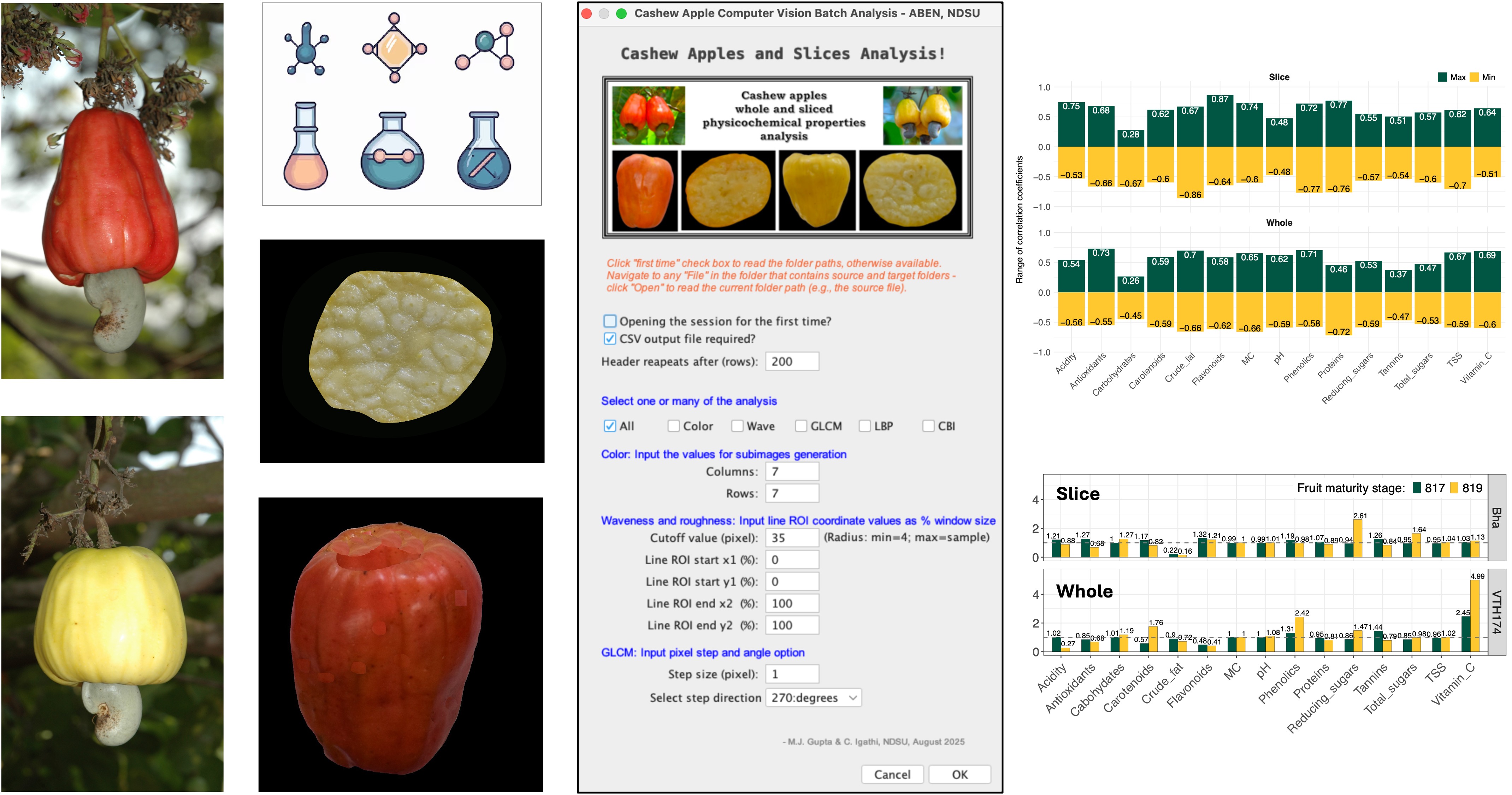
The developed plugin, titled “Cashew Apple and Slices Analysis”, features an input panel depicted in Figure 6. The panel provides the user interface for various methodologies and enables the input of various parameters for the analysis. The input panel is designed to be self-explanatory with brief instructions, distinct checkboxes, and input fields categorized by types of analysis. Users interact with the panel to generate analysis and output. This plugin operates in a “batch-mode”, where all the preprocessed images stored in the input folder are automatically analyzed, results are appended with timestamps and stored in a ‘csv’ file format for record and further analysis, and visualize the results progress of batch analysis as a pop-up window (Figure 5D1) and on the ImageJ progress bar.
The plugin (Figure 6) provides user-friendly prompts to ensure accurate input. The first checkbox, “Opening the session for the first time?”, establishes the default folder for storing input images during batch processing, a task that is necessary only once. When the ‘csv’ output is desired, the second box should be checked. The type of analysis desired can be chosen from the group of checkboxes: All, Color, Wave, GLCM, LBP, and CBI. Users can choose the analysis individually or in combination, or ‘All’ (ignores individual analysis and generates all analysis results). The other inputs (input boxes) are related to the different analyses and are explained in Section 2.3.3. Upon clicking the “OK” button, the program executes based on the selected analysis and generates images, log files, and CSV data. The “Cancel” stops the execution, bypassing it, and makes the plugin ready for the next session.
2.3.5. The Cashew Apples and Slices Analysis plugin
The “Cashew Apples and Slices Analysis” ImageJ plugin has a total of 2050 lines coded in Java using Fiji (Ver. ImageJ 1.54q). The plugin’s functionality is encapsulated within various Java methods (functions), including reading inputs, performing different analyses, and generating graphical and textual outputs, which play well with the batch processing strategy used in the plugin. Some of the advanced features used in the plugin are derived from packages including Apache Commons DescriptiveStatistics; ImageJ’s ImagePlus, ImageProcessor, GenericDialog, GaussianBlur, WindowManager; and Java’s Stream, Date, File, BufferedWriter, FileWriter.
2.4. Data analysis for predicting the wet chemistry from image-based parameters
Data analysis is aimed to (i) determine the strength of association between the wet chemistry physicochemical properties (dependent) and the image-based parameters (independent) variables and graphically visualize the correlation, (ii) evaluate the range and ranking of image-based parameters correlation to wet chemistry parameters, (iii) develop the top three linear prediction models of wet chemistry based on the image-based parameters, and (iv) perform prediction and validation with visualization, employing the top-ranked prediction model developed and applied to unseen images. To accomplish these aims, an R (Ver. 4.5.1, 2025) program was developed utilizing the RStudio IDE (Ver. 2025.09.1, Posit Software, PBC). Major R packages involved in the R program development are tidyverse, dplyr, readr, corrplot, and ggplot2. The R program was coded as an assembly of several “functions”, each designed to perform specific tasks. These functions were appropriately invoked in the program to execute the analysis and visualization. A brief description of the various data analysis procedures is presented subsequently, and the R script containing the data is uploaded to an online data repository [39].
2.4.1. Correlation analysis and visualization
The data obtained from the measured wet chemistry parameters and generated by the computer vision plugin (Section 2.3.4) as an *.csv file, forms the input for the correlation analysis. The program reads the entire csv file and converts it into a “dataframe”. The data should be preprocessed by subsetting to extract the relevant variables, discarding other informative (e.g., time, image file name) and non-varying (e.g., certain minimum and maximum values) parameters (Section 3.2). The subset data contains categorical variables, namely, cashew apple varieties (6), maturity stages (2), and sample types (2), along with their replications. The replications should be combined into mean values associated with unique combinations of the categorical variables. The analysis is performed separately for the slice and the whole samples (as their images exhibit distinct differences). These operations were carried out through group_ by, filter, and select operations.
A matrix of correlation coefficients (r) was generated using the cor() command, and this object, after being converted to a dataframe, was output as a csv file for further analysis using the write_ excel_ csv commands. The corrplot() command with method of “square” and color options created the r values visualization through a color-coded correlation diagram (Figure 7). Correlation diagrams were created separately for the slice, whole, and combined samples to study their effect on the association.
2.4.2. Range and ranking of correlation coefficients
Although feasible with R, the MS Excel spreadsheet program was utilized to create the range data (Section 3.5) and ranking of r values. In addition, code for generating a LATEX ranking table was created (Section 3.6). Utilizing the MIN() and MAX() functions on the slice and whole samples *.csv files separately, the r range data was generated, excluding the r values of wet chemistry parameters (self-correlation). The generated range data was then read into the R program, reshaped using pivot_ longer, and plotted using ggplot commands. The ggplot utilized geom_ bar with the “stack” option to draw the range maximum and minimum r values, facet_ warp, and other commands to depict both slice and whole samples.
For developing the ranking table, the actual r values (both +ve and -ve) were (i) converted to absolute values using the ABS(), (ii) for each wet chemistry parameter, the image-based parameters were ranked using the RANK(), (iii) the top 10 image-based parameters for each wet chemistry parameter were collected after sorting, and (iv) those top ten image-based parameters as text were combined using the CONCATENATE() with other symbols (e.g., & and \\) to generate the LATEX table code.
2.4.3. Wet chemistry prediction models development
The process of creating the top three (3) models for each wet chemistry parameter (15) with maturity stages (2) and sample types (2) from the single master subset data (total = 180 models; Section 3.7) involves a series of intricate operations. The data processing requirements to achieve this as a “repetitive” function are: select the specific wet chemistry variable while dropping the other 14; select all of the image-based parameters; filter the rows that contain the desired maturity stage and sample type; create a set of linear models using the lm() function for all the image-based parameters by generating a formula for the dependent with all the image-based parameters predictor variables using the map() function that generates a “list” of models; extract the intercept, slope, , number of observation, and individual formula strings using the sapply() function; generate a dataframe with these values; sort the models based on in desending order using arrange(-()); and select the top three models using slice_ head(n=3). This function was invoked 60 times (15 wet chemistry × 2 stages × 2 sample types), and each time it produced the top three models (3 rows). These three rows of output were appended to generate the 180 model result rows using bind_ rows and finally written to the file using write_ excel_ csv() command.
2.4.4. Wet chemistry prediction and validation
For prediction, the top-performing models of wet chemistry in each combination of stage and sample type (60) were utilized across the test set of unseen images. The predictions are validated with the known wet chemistry measurements for the six varieties of cashew apple. The image-based parameters were generated by the developed plugin with the test images as inputs. The top-performing models in each category will specify the independent variable involved, and the value of that variable will be obtained as a mean from the image-based parameters plugin results. The mean value of the independent variable when input into the linear model with specific slope and intercept values will generate the prediction of wet chemistry physicochemical properties. The performance of prediction will be evaluated as the ratio (predicted to actual), where the ideal prediction will have a ratio of 1.0, while underestimation will have ratios <1.0 and overestimation will have ratios >1.0.
The prediction and validation can be visualized as a dodged bar graph with maturity stages for all the wet chemistry properties evaluated for each sample type. The six varieties will be depicted as facets. The dodged bar plot function takes the data (actual, predicted, and ratio, specific to slice and whole), and y-axis limits (min and max) inputs, and generates the plot. The plot function filters the ratios, the geom_ bar() command takes “dodge” as argument, passes the y-axis inputs into the ylim() command, draws a horizontal line at using geom_ hline with yintercept = 1.0, and makes facets using facet_ wrap() with ∼Variety as the argument. The online data repository R script provides additional details [39].
3. Results and discussion
3.1. Results: Variation in wet chemistry results within samples and varieties
Significant differences were observed in physicochemical properties of cashew apples between maturity stages 817 and 819 across all varieties (mean ± std shown in Table 3; wet chemistry measurement protocols are given in Appendix A). With the progress of maturity stages, the acidity decreased while the pH and TSS increased consistently (). Antioxidant activity, flavonoids, phenolic content, and tannins showed significant reductions (), indicating a decline in bioactive compounds after maturation. Carbohydrate content, reducing sugars, and total sugars increased significantly at stage 819 (), suggesting an increase in sweetness and energy value. Carotenoids and vitamin C also increased sharply, particularly in Bhaskara and VRI-3 varieties (). Crude fat content and proteins declined across all varieties, with VTH-174 and MDK showing the most pronounced reductions. The variety VTH-174 exhibited the highest antioxidant activity at stage 817. Bhaskara recorded the highest vitamin C content at stage 819 (181.71 mg/100). Variety VRI-3 showed a threefold increase in carotenoids from stage 817 to 819, and NRCC-1 had the highest sugar and total carbohydrate levels at stage 819.
Overall, significant fluctuations in the biochemical composition of cashew apples were observed between maturity stages 817 and 819, reflecting the typical ripening dynamics (Table 3). The decline in phenolics and flavonoids suggests reduced antioxidant activity with maturity (negative correlation between these compounds and fruit ripening), as reported in previous studies [63]. Conversely, the increase in sugar and vitamin C content indicates that with ripening, the palatability and nutritional appeal of cashew apples are improved. This is particularly evident in varieties Bhaskara and VRI-3. Therefore, it is expected that any visual or textural differences identified at these stages could be correlated with these biochemicals.
The selected quality parameters are essential for assessing the quality of the fruit; however, these methods are destructive in nature. All parameters require special instruments and an elaborate extraction procedure of the samples for analysis. Total phenols, tannins, flavonoids, antioxidant activity, sugars, carbohydrates, vitamin C, and carotenoids require solvent-based extraction of the targeted compounds followed by spectrophotometric or titrimetric estimation. Extraction and estimation process demand additional time and the use of expensive solvents and chemicals for analysis, especially for total phenols, tannins, flavonoids, antioxidant activity, sugars, carbohydrates, and carotenoids. Parameters such as carbohydrates, protein, and fat estimation involve extended extraction and thus require more time for estimation. Additionally, estimation of many of these quality parameters requires the use of chemicals, which are corrosive and harmful to skin and eyes, which may also lead to systemic injury.
3.2. Independent image-based variables considered for analysis
By executing the developed ImageJ plugin with for a set of user inputs (Figure 6) with the training (75%) batch of images of cashew apple samples (6 varieties; 2 sample types; 2 sample stages; 7–13 slice replications/variety; 4–6 whole replications/variety; 104 slices + 60 wholes; 164 total), the exhaustive 144 image-based parameters output was generated. Upon analyzing the variations of these parameters across the 15 wet chemistry physicochemical properties variables (dependent), several of the image-based variables (independent) exhibited no or insignificant variation. Therefore, the following set of 28 parameters was excluded (abbreviated names provided and expanded form presented in Table 1 for further analysis and model development: Ov-mxR, Ov-mxG, Ov-mxB, Ov-miR, Ov-miG, Ov-miB, Rn-Gmn, Ov-noR, Ov-noG, Ov-noB, Wn-no, Rn-no, L-pxGr, L-pxR, L-pxG, L-pxB, L-miGr, L-mxGr, L-medGr, L-miR, L-mxR, L-medR, L-miG, L-mxG, L-medG, L-miB, L-mxB, and L-medB. It should be noted that these parameters, when considered, would have resulted in the least correlation and have not generated practical models or those with the lowest performance. Thus, only the rest 116 image-based parameters () were used for further analysis.
3.3. Plugin input variables combination selection
Given that user inputs and their combinations (Figure 6) influence the image-based parameters evaluated, the best inputs must be selected based on the collective performance of the prediction models. Even though five sets of image-based parameters, including color, waveness and roughness, GLCM, LBP, and color indices, were evaluated (Table 3), the input variables were only from the three sets (Figure 6), while other inputs were internally configured within the plugin. A systematic approach was employed to evaluate and identify the most suitable combination of input variables (color: columns and rows; waveness and roughness: cutoff value; and GLCM: step size and step direction) entered through the plugin’s input panel (Figure 6). Every combination of the input parameters for the 4 categorical variables (types and stages), 15 dependent wet chemistry variables, with the 116 dependent parameters resulted in the generation of a total of 6960 () simple linear models generated internally. However, considering only the top three, totaling 180 (), models within each category were utilized for further analysis. The sum of the coefficient of determination () of the top three 180 models (), with the largest value serving as an indicator for selecting the most suitable combination of input variables (Table 4).
Therefore, initially the color inputs, namely the grid size, were varied to , , , , , and , while keeping the other inputs at their starting values. It was observed that the values attained their peak at and subsequently declined. Now keeping as a constant input for color inputs, the waveness and roughness Gaussian filter radius was gradually varied to 4, 5, 10, 15, 20, 25, 30, 35, 40, and 50 pixels. The effects of these variations were recorded, and the 35 pixels yielded the best outcome (Table 4). Keeping these two inputs constant, the GLCM step size was varied gradually to 1, 2, 3, 5, and 10 pixels, which revealed that the 1 pixel step size was the best. Proceeding similarly, a combination of 4 GLCM step direction angles (0°, 90°, 180°, 270°) was studied, and found that 270° was the best (Table 4). To further validate the effectiveness of the color grid size in conjunction with the selected input combination, the models were subjected to testing for , , , a step above and below the considered , which reaffirmed its effectiveness with the highest value of of 76.437 (Table 4). Consequently, the best plugin input combination that is used for further analysis is: a color grid size of , a waveness and roughness cutoff of 35 pixels, a GLCM step size of 1 pixel, and a GLCM step direction of 270°. The CPU processing time for this combination was image (HP ZBook Fury 16-inch G11 Mobile Workstation PC; Intel® Core™ i9 13950HX 5.5 GHz, 32 GB RAM, 1 TB storage).
The results underline the importance of input selection in modeling with multiple variables. The optimization strategy—based on cumulative values, proved effective in isolating input combinations that maximized the predictive performance across the multiple dependent variables. This approach is particularly valuable when dealing with complex systems where interactions among variables are non-linear or context-dependent. This methodology offers a framework for model refinement. Thus, by iteratively evaluating input combinations, one could converge on combinations that yield the most reliable and generalizable models. However, caution should be exercised when using as a heuristic for input selection, as it may not fully capture nuances such as overfitting, multicollinearity, or model interpretability. Therefore, further research on additional criteria such as adjusted , or cross-validation error, etc., is necessary. Additionally, applying a larger data set (with more varieties and maturity stages), and non-linear modeling techniques may enhance the predictive capacity where linear assumptions are insufficient.
3.4. Visualizing Correlation—Correlation Diagram And Absolute Correlation Coefficients
Pearson’s correlation coefficient (r) quantifies the strength and direction of 15 wet chemistry physicochemical properties with the 116 image-based parameters, and themselves were evaluated using the input combination (; 35 pix; 1 pix; 270°; Section 3.3) and visualized in the form of a correlation diagram (Figure 7). The correlations were calculated separately for (i) all sample types combined, (ii) slice images only, and (iii) whole fruit images only to determine the effect of the sample type category during model development. Table 5 presents the sum and mean absolute correlation coefficient () values, which facilitate the comparison of the performance of sample types and groups of parameters. The correlation results (Figure 7 and Table 5) indicate that combining both sample types is not an effective strategy (). Although keeping the types separate yielded a better correlation, the slice () performed superiorly compared to the entire sample ().
3.4.1. Interrelationships among wet chemistry parameters
Overall, the correlation diagram (Figure 7; separated by a solid horizontal line) shows better intercorrelation among wet chemistry variables compared to the image-based parameters, evident from the darker-colored tiles with wet chemistry. This observation is corroborated by the absolute mean of 0.433, which is greater than the range of 0.128–0.324 observed for the image-based parameters (Table 5). Strong interrelationships were observed among key physicochemical properties, specifically between crude fat, vitamin C, antioxidants, and total phenol content; carbohydrates and total sugars; carotenoids and total sugars; as well as tannins and antioxidants. These robust associations also suggest, apart from serving as direct predictors, that certain physicochemical properties may serve as indirect predictors for others, which can be beneficial in gaining insights into other parameters. For example, if vitamin C shows poor correlation with texture features but is strongly linked to crude fat, then crude fat, if reliably predicted from image-derived parameters, could act as a proxy for estimating vitamin C levels. Despite these specific advantages of direct prediction of physicochemical properties from others, the wet chemistry determination is time-consuming and highly expensive.
This strategy of leveraging internal biochemical correlations to enhance predictive modeling aligns with previous studies. Hasanzadeh et al. [64] demonstrated that hyperspectral imaging combined with regression analysis could accurately estimate apple quality traits such as pH, soluble solids, and titratable acidity, with correlation coefficients exceeding 0.99. Similarly, Paulo et al. [65] demonstrated that visual descriptors extracted from fruit images captured in uncontrolled environments could be mapped to physicochemical parameters using non-linear regression models, thereby effectively estimating fruit maturity.
3.4.2. Correlation between wet chemistry and image-based parameters
The five groups of image-based parameters collectively had a lower correlation with wet chemistry compared to the intercorrelation of wet chemistry. While all sample images of image-based parameters were consistently low, the slice and whole samples were the best for certain groups (Table 5). For example, slices exhibited better correlation with waveness and roughness, LBP, and color indices, whereas wholes exhibited better correlation with the color grid and GLCM.
Among the image-based parameters group methodologies, slice sample images exhibited the highest correlation with surface morphology (waveness and roughness; ), followed by color indices (), and whole samples color grid (), followed by GCLM () and LBP () were the best (Table 5). It is interesting to note that the color indices, which are easy to obtain as they are derived solely from R, G, and B values, also exhibit favorable correlation for slice and whole samples (). This observation can be visualized in the correlation diagram (Figure 7) with methodology groups separated by dotted horizontal lines and darker color patches. Correlations derived from the whole fruit sample images indicated that, although associations were generally stronger than the combined dataset, they were consistently weaker than those observed for slice images. Notably, several wet chemistry parameters, including vitamin C, TSS, total sugars, crude fat, and moisture content, exhibited moderately higher correlations with GLCM contrast and roughness-based texture metrics.
Overall, the for image-based parameters for slice, whole, and combined samples were 0.268, 0.252, and 0.197, respectively, which is lower than the inter-correlation of wet chemistry value of 0.443 as observed previously. Collectively, these findings reinforce the potential of image-based parameters employing computer vision analysis not only for direct prediction of physicochemical properties but also for inferring quality parameters through correlated biochemical proxies. Thus, it expands the scope for the development of non-destructive quality assessment tools in postharvest and processing operations.
3.5. Correlation analysis of wet chemistry with image-based parameters—value ranges
The range of r for all the 116 image-based parameters (independent variables) against the 15 wet chemistry (dependent variables) for the finalized input combination, grouped by sample types (slice and whole) is presented in Figure 8. These categories are distinct from the image viewpoint, and their correlations are treated separately (Table 5). For slice samples, r ranged from to 0.87, indicating both strong negative and positive associations. In contrast, for whole samples, the range was slightly lower and narrower, from to 0.73, suggesting that the independent parameters computed based on slice images exhibited enhanced sensitivity to the image-based parameters.
Contrasting the association of wet chemistry parameters with image-based parameters between sample types (slice and whole), the parameters derived from slice images revealed stronger correlations for most parameters and in “internal quality” traits, particularly those related to biochemical composition (e.g., flavonoids, crude fat, proteins, total phenolics content, acidity, and moisture content). This supports our hypothesis that exposing internal tissues (through slice images) enhances the accuracy of indirect measurements, especially for parameters not uniformly distributed across the fruit. Whole fruit images favored parameters linked to “external features” (e.g., antioxidant activity and vitamin C), but underperformed for most internal chemical traits. The reduced correlation range suggests that whole fruit assessments may require more advanced imaging or hybrid sensing techniques to improve predictive power. The observed correlation patterns underscore the potential of using image-based data to predict wet chemistry traits, especially with images of sliced fruits is feasible. For improved correlation, a larger sample size for training may account for better results.
For slice sample images, the most strongly correlated dependent parameters () estimated were flavonoids (0.866), crude fat (), proteins (0.772), total phenolic content (), acidity (0.749), moisture content (0.736), and TSS (). The least correlated parameters were pH, tannins, reducing sugars, and total sugars, with coefficients of , , 0.553, and 0.566, respectively. For whole fruit sample images, the most strongly correlated dependent parameters were antioxidant activity (), proteins (), and total phenolics (0.706). The moderately correlated parameters were crude fat (0.696), vitamin C (0.691), TSS (0.666), moisture content (), and pH (0.623). The least correlated variables were total carbohydrates, tannins, total sugars, reducing sugars, and carotenoids, with correlation coefficients of , , , , , respectively.
Overall, among the wet chemistry parameters, flavonoids and crude fat consistently exhibited high correlation () with the plugin image-based parameters. Proteins, total phenolic content, acidity, moisture content, antioxidant activity, carotenoids, and TSS demonstrated moderate to strong correlations ( to 0.77) with texture and color-based parameters, especially where internal tissue exposure improves detection. Total carbohydrates, tannins, total sugars, and reducing sugars showed weak correlations () across most independent variables, suggesting limited predictability from image-based non-destructive measurements. Furthermore, the correlation coefficients between dependent and independent variables were consistently higher for slice-derived independent parameters compared to those obtained from whole-fruit images. Focusing on analyzing the dynamics of the maturity stages, varieties, and collecting more samples could contribute to improving the association between the independent and dependent parameters.
3.6. Top ranking image-based parameters correlation coefficients
To identify the most influential image-based parameters predictors for each wet chemistry physicochemical properties trait, they were ranked based on their Pearson correlation coefficients, and the top ten features of wet chemistry categorized by sample type (slice and whole), are presented in Table 6. This ranking framework enabled the identification of dominant image patterns and feature categories associated with specific chemical and physical attributes of the fruits. In general, slice and whole samples had a distinctly different set of top-ranking parameters for the same fruit physicochemical properties due to differences in color, texture, and morphology.
Among the 150 top 10 ranked image-based parameters for slice samples (15 wet chemistry × 10 ranks; Table 6), the surface methodology covered 52.0% followed by color indices (25.3%), color grid (14.0%), GLCM (4.7%), and LBP (4.0%); and for whole samples surface methodology covered 38.0% followed by color grid (32.6%), color indices (14.7%), LBP (8.7%), and GLCM (6.0%). Across the 15 physicochemical properties, surface morphology descriptors (waveness and roughness metrics) consistently ranked among the top predictors, followed by color-based indices or grids, and finally GLCM and LGB methodologies with similar low performance. Among these top-ranked parameters, the color indices developed in this study (17; Table 2) performed well. The total number of color indices featured in the top-ranking 150 parameters was 22 for each slice and whole sample (Table 6). Out of these, the number of indices developed in this study was 9 for the slice and 3 for the whole samples. This, out of the total 150, was 6.0% (slice) and 2.0% (whole), and out of color-based indices was 40.9% (slice); 13.6% (whole), indicating a significant performance of the indices developed in this study.
Color-based indices methodology, which is easy to derive, also showed strong associations with biochemical properties such as phenolics and carotenoids, indicating that reflectance captured in RGB images can serve as a proxy for phenolics and carotenoids profiling. Color grid methodology parameters (e.g., mean, median, STD of blue, green, and blue channels) were particularly informative for sugar-related traits such as TSS, total sugars, and reducing sugars. Acidity and pH had dominating associations with surface morphology-based parameters and color-based indices. These results agree with earlier studies [66,67] that have demonstrated a direct correlation between color values and textural properties are directly correlated to various physicochemical properties such as acidity, pH, and phenolics.
3.7. Wet Chemistry physicochemical properties Prediction Model Development
The Table 7 presents the top three models, assessed based on the model performance parameter , for each wet chemistry physicochemical properties parameter across all sample types and maturity stages (total = 180 models; Section 3.3), from the complete set of 116 image-based parameters independent variables. It is important to note that image-based parameters featuring in the top models (based on ; Table 7) may differ from the top ten highly correlated image-based parameters (based on r; Table 6). This is because there are differences in the linear model fitting and Pearson’s correlation evaluation. While the correlation coefficient evaluates the strength of association between the independent and dependent variables, the model development provides the actual tool used for making the final prediction. Therefore, the latter (Table 7) is more suitable for the objective of the study.
Across all the wet chemistry physicochemical properties parameters, the values, which represent the models’ performance, ranged from as high as 0.936 to as low as 0.167 for both maturity stages, indicating varying degrees of predictive strength depending on the dependent parameter, sample type, and maturity stage categories. For slice samples, the mean values for stage 817, stage 819, and both are , , and ; and these whole samples are , , and , respectively. The mean for the samples and stages combined is . Considering the better-performing models (), it was found that slices covered 24.4% with stage 817 and 51.1% with stage 819, and for wholes 6.7% and 13.3% coverage, respectively. These results indicate that the slice images and ultimate maturity stage of 819 are the most effective for evaluating the wet chemistry, hence recommended for the computer vision analysis of physicochemical properties analysis. This combination will also yield 24.4% of high-performance models (). When whole samples are required, the ultimate stage of 819 should be chosen again.
The models of slice and the maturity stage 819 combination () will cover 11 out of 15 (73.3%) wet chemistry physicochemical properties. These wet chemistry properties that can be successfully modeled are: acidity, antioxidant, carbohydrates, carotenoids, crude fat, flavonoids, pH, phenolics, proteins, tannins, and vitamin C. The wet chemistry properties covered by whole samples were only five (acidity, carbohydrates, carotenoids, proteins, and vitamin C), which is a subset of the “slice+819” combination. The “slice+817” combination covered again five wet chemistry properties (carotenoids, crude fat, pH, TSS and and vitamin C), whereas the property TSS was the unique addition to the list of slice and 819 combination. From the effort and complexity viewpoint, TSS is a relatively simple and quick measurement using a refractometer. Therefore, the recommendation of the “slice+819” combination, along with more sampling closer to the ultimate maturity stage, will effectively deliver the wet chemistry physicochemical properties through the simpler image-based computer vision methodology developed.
yellow
3.8. Wet Chemistry physicochemical properties Prediction Models Validation
A systematic validation strategy was employed using approximately 25 percent of the reserved (test) data to assess the performance of developed models (based on 104 slices + 60 wholes = 164 images; Figure 6 and Section 3.7). The testing batch (unseen) of images of cashew apple samples (6 varieties; 2 sample types; 2 sample stages; 2–3 slice replications/variety; 2 whole replications/variety; 30 slices + 24 wholes; 54 total), were processed through the ImageJ plugin with the finalized inputs to generate the image-based parameters and the wet chemistry physicochemical properties were predicted using the topmost model (Table 7). Predicted wet chemistry parameters are compared with their actual values (Table 3), and the deviation expressed in terms of ratios (predicted/actual) are visualized as a paneled dodged bar graph across wet chemistry parameters, with maturity stages and cashew apple varieties (Figure 9).
Ideally, a ratio close to 1.0 indicates high predictive fidelity, while deviations highlight (<1.0) under- or (>1.0) over-estimations (horizontal dotted lines in Figure 9). Extreme values <0.75 or >1.25 depict poor prediction accuracy or model bias. For the 360 predictions (15 wet chemistry × 2 stages × 2 types × 6 varieties), the mean ratio for slice () and whole () were comparable, indicating similar prediction performance. Within the acceptable prediction ratio range of 0.75 to 1.25, a 66.7% for slice and 60.6% for whole samples demonstrate that a predominant number of predictions fall in this range, and slice performs better than whole samples. The under- and over-estimations by the models beyond this range were 14.4% and 18.9% for slice and 18.3% and 18.9% and 21.1% for whole samples, respectively.
Upon comparing the effects of maturity stages, the mean ratio of stage 819 (slice: 1.069; whole: 1.029 ) is closer to the ideal ratio of 1.0 than that of stage 817 (slice: 1.092; whole: 1.129) from 90 predictions each (Figure 9). This prediction result supports the idea that the ultimate maturity stage of 819 will be more favorable for the methodology, which was already anticipated from the analysis of the developed prediction models (Table 7).
Within the high prediction range of the ratio between 0.85 and 1.15, the wet chemistry physicochemical properties of moisture content and TSS had a perfect count of 12 for both maturity stages and sample types. The subsequent five wet chemistry parameters are carbohydrates, pH, proteins, and total sugars, featuring in both stages and sample types (6–11 out of 12). This result suggests a strong model generalization for these traits. The least prediction performance was exhibited by phenolics, antioxidants, crude fat, flavonoids, tannins, and vitamin C (2–3 out of 12), both for slices and wholes. It is interesting to note that carotenoids can be predicted using slices (5/12) but cannot be predicted by whole samples (1/12) based on the analysis results.
3.8.1. Study’s Limitations and Suggestions for Future Work
Several limitations were identified and will be encountered by users when reproducing this research in terms of experimentation and computer vision methodology development. Obtaining a suite of wet chemistry data for several varieties of cashew apple is expensive, time-intensive, and sometimes not affordable. The study utilized only six varieties at two maturity stages, resulting in the utilization of only six data points for each model developed (180 total). Therefore, this should be considered when applying the models. The study utilized only natural lighting during the image data acquisition, and this would have created some variation and affected the prediction accuracy. Developing new methodologies beyond those presented in the study requires a high level of computer vision and image analysis programming skills.
These limitations, in fact, present opportunities and guidance for future research in this knowledge domain. Expanding the dataset can assist in identifying and correcting outliers prior to training, thereby reducing the risk of skewed predictions. A larger dataset could also support more robust calibration across different varieties and development stages, ultimately enhancing the models’ performance. Incorporating non-linear modeling approaches, along with increased data volume, may further enhance models’ predictive performance. Color calibration of the input images will address and mitigate the variations induced by ambient lighting, potentially improving the computer vision analysis methodology. The current approach can be further optimized by integrating additional analytical techniques (e.g., textural features, color indices, other surface morphologies) as well as other relevant wet chemistry properties into the computer vision ImageJ plugin. The developed methodology can be applied to the evaluation of the wet chemistry physicochemical properties of other horticultural crops. As the results revealed that the optimal maturity stage was 819, it is feasible to develop an intermediate maturity stage, such as 818 (between stages 817 and 819), to expand the time window available for harvest, measurement, and analysis. Also, integration of the methodology with machine learning (ML) and artificial intelligence (AI) could enable universal, in-vitro tools for rapid fruit analysis and postharvest automation. These aspects will constitute a great potential for future research and can contribute to the enhancement of the overall performance of the computer vision methodology for indirect wet chemistry physicochemical properties measurements.
4. Conclusions
This study successfully developed a vision-based methodology for assessing 15 physicochemical properties of cashew apples, which are conventionally evaluated through wet chemistry protocols, across six diverse varieties and two maturity stages from the images of slices and whole samples. From the wet chemistry evaluation of physicochemical properties, significant changes were observed between maturity stages 817 and 819 across all varieties, which reflect variety-dependent ripening dynamics and support the use of biochemical markers for quality assessment. The alternative methodology of a developed user-coded and user-friendly computer vision ImageJ plugin, employing five image-based methodologies (color grid, surface morphology, GLCM, LBP, and color indices), analyzed the input images of slices and whole cashew apple samples, in batch processing mode, and generated 144 image-based parameters parameters for further analysis (correlation, linear models, predictions). Optimal input configuration for the plugin was color grid: 7; waveness and roughness cutoff radius: 35 pixels; GLCM sampling size: 1 pixel; and GLCM angle: 270°. The plugin execution was rapid, clocking a CPU time of about image (Intel® Core™ i9 13950HX 5.5 GHz, 32 GB RAM).
The correlation between the image-based parameters (independent) with wet chemistry (dependent) traits, exhibited stronger correlations for slice-based image variables ( to ; ) compared to that of whole fruit images ( to ; ) indicating enhanced sensitivity to internal quality features. Strong inter-correlations among wet chemistry properties ( to ; ) indicate that reliably predicted parameters can effectively serve as proxies for those with weaker image associations, thereby reinforcing the potential of image-based analysis and biochemical surrogates for non-destructive quality assessment. Surface morphology (52% & 38%), color indices (25.3% & 14.7%), and color grid (14% & 32.7%) features consistently ranked as top predictors across physicochemical properties, with slice and whole fruit images revealing distinct yet complementary patterns. The color indices developed in the study contributed significantly, featuring among the top-ranking 150 parameters (6.0% & 2.0%), and among the 22 color-based indices (40.9% & 13.6%). This ranking framework highlights the potential of easy-to-evaluate RGB descriptors for their non-destructive estimation.
The developed models for the slice at the maturity stage 819 () covered 73.3% (11 out of 15) wet chemistry physicochemical properties and successfully modeled acidity, antioxidant, carbohydrates, carotenoids, crude fat, flavonoids, pH, phenolics, proteins, tannins, and vitamin C. In contrast, the wet chemistry properties covered by whole samples were 33.3% (5 out of 15; acidity, carbohydrates, carotenoids, proteins, and vitamin C). The combination “slice+819”, along with more sampling closer to the ultimate maturity stage, is recommended to effectively deliver the wet chemistry properties through the developed simpler image-based computer vision methodology.
From the prediction and validation of the developed model using the unseen image data, 66.7% for slice and 60.6% for whole samples belonged to the prediction ratio range of 0.75 to 1.25, demonstrating model validity. Models of the slice samples performed better than the whole samples. The wet chemistry properties predicted by the models in the decreasing order of performance were moisture content, TSS, carbohydrates, pH, proteins, and total sugars; and those with the least prediction performance were phenolics, antioxidants, crude fat, flavonoids, tannins, and vitamin C. Suggestions for future research include a larger dataset across different varieties and maturity stages; exploring non-linear modeling approaches; performing color calibration of the input images; incorporating additional wet chemistry and analytical techniques; developing an intermediate maturity stage; extending this methodology to other horticultural crops; and integrating it with modern ML and AI techniques.
Author Contributions
Conceptualization, M.J.G., C.I., and J.N.; methodology, M.J.G., C.I., and J.N.; formal analysis, M.J.G., C.I., J.N., A.J., H.T., S.S., A.M., J.D.A., and P.K.; investigation, M.J.G., C.I., J.N. A.J., H.T., S.S., A.M.; J.D.A., and P.K.; resources, M.J.G., J.N., J.D.A., P.K., and C.I.; data curation, M.J.G., and C.I.; writing-original draft preparation, M.J.G., J.N., and C.I.; writing-review and editing, M.J.G, J.N., C.I., A.J., H.T., S.S., A.M., P.K., J.D.A., and S.R.; visualization, M.J.G., C.I., and J.N.; supervision, M.J.G., J.N., and C.I.; project administration, J.N., J.D.A., M.J.G., and P.K.; funding acquisition, J.N., and J.D.A., All authors have read and agreed to the published version of the manuscript.
Funding
This work was supported by the Indian Council for Agricultural Research, Project ID.No: IXX20122, Project title: Enhancing the shelf life of cashew apple to increase the market potential and development of functional foods.
Institutional Review Board Statement
Not applicable.
Data Availability Statement
The image data used in the manuscript is available from Mendeley Data, V1, at https://doi.org/10.17632/67kn43rj5c.1 (accessed on 18 October 2025). This dataset is cited in the manuscript as [39]. This dataset contains three files, namely, (1) Raw input images, (2) Wet chemistry data of cashew apples, and (3) R script used for analysis in the study.
Appendix A
Appendix A.1. Physicochemical properties
(i) Moisture, protein, and fat
Moisture content in cashew apples was determined by following the ISO 712:1998 method with a gravimetric principle using a hot air oven. The protein was estimated by following the Kjeldahl method as described by the AOAC method (920.151) [68], where a Kjeldahl apparatus (DX VATS, Pelican, Kelplusclassic, 2015) was used for digestion, distillation, and titration. For crude fat estimation Soxhlet apparatus (KSEA-1B, KEMI) was used, and samples were subjected to fat extraction using n-hexane. The extraction was carried out for approximately 3 , and the percentage of fat was calculated as per the AOAC method (920.39).
(ii) Total soluble solids, pH, and titratable acidity determination
Total soluble solids (TSS) were analyzed based on the AOAC method (932.12) using a portable hand refractometer corrected for . The AOAC method (981.12) was also used for determining the pH of the fruit. The AOAC method (942.15) was followed for assessing the titratable acidity (TA) of cashew apples, and results were expressed as percentage acidity in terms of citric acid.
(iii) Total carbohydrate
Total carbohydrate was estimated spectrophotometrically using the anthrone method [69], where the sample was hydrolyzed using 2.5N HCl for 3 in a boiling water bath. After cooling to room temperature, it was neutralized with Na2CO3 until the effervescence ceased. The solution was centrifuged after adding 10 mL of distilled water. The supernatant was collected, and the volume was made up to 100 mL with distilled water. Total carbohydrate was analyzed by adding 4 mL of anthrone reagent to a mixture of 0.1 mL aliquot and 0.9 mL distilled water. The mixture was incubated in a boiling water bath for 8 and cooled to room temperature. The green to dark green color developed was measured using a spectrophotometer at 630 nm. With spectrophotometry methods, the sample values are measured indirectly with reference to a standard solution of known concentration. A standard curve was prepared by plotting the absorbance values of standard glucose solutions. The concentration of carbohydrate is calculated as:
(iv) Total sugar
Total sugar content in cashew apple samples was determined using the Hedge and Hofreiter [70] spectrophotometric method. Sugars were extracted by mixing the samples with 80% hot ethanol and were refluxed for 1–2 . The mixture was filtered, and the ethanol was removed using a rotary evaporator. The volume of the filtrate was made up to 100 mL. An aliquot (0.1 mL) was mixed with 0.9 mL distilled water and 5 mL anthrone reagent. The solution was then incubated at for 11 and the absorbance was read at 630 nm. D-glucose was used as a standard, and the results were expressed as a percentage on a fresh weight basis.
(v) Reducing sugar
Reducing sugar was estimated using the dinitro salicylic acid (DNSA) method [71]. Briefly reducing sugars were extracted from the samples as described for total sugars using 80% hot ethanol. A 3 DNSA reagent was added to 1 aliquot and incubated in boiling water bath for 16 . The mixture was then cooled to room temperature, and the volume was made to 25 mL with distilled water. The absorbance of the sample was read at 575 nm using a spectrophotometer. The reducing sugar content was calculated from the calibration curve of standard D-glucose, and the results were expressed as a percentage on a wet basis.
(vi) Vitamin C (ascorbic acid) estimation
Vitamin C was determined using the 2,6-dichlorophenolindophenol (DCPIP) method (AOAC Method, 967.21). The samples were extracted using 3% metaphosphoric acid to obtain a solution of vitamin C. The extract was titrated with a standardized DCPIP solution until a pale pink color appeared. The results were expressed as mg/100 of ascorbic acid on a wet basis.
Appendix A.2. Biochemical Properties
For the estimation of biochemical properties, polyphenolics were extracted as described by Ramful et al. [72] with some modifications. Approximately 1 of pulp was extracted using 10 mL of 80% ethanol. The extract was sonicated for 30 t and then centrifuged at 10,000 Xg for 10 at and the extract was decanted. The residue was extracted twice following the aforementioned procedure. The combined extracts were adjusted to 30 mL and were filtered with a 0.4 nylon filter. The filtered extract was stored at and used for the determination of total phenol, total flavonoids, antioxidant activity, and tannins.
(i) Total phenolic content (TPC)
TPC was estimated spectrophotometrically using the Folina Ciocalteu reagent (FCR) [73]. The aliquot (0.1 mL) was mixed with 2.9 mL of deionized water, 0.5 mL of Folin Ciocalteu reagent, and 2.0 mL of 20% Na2CO3 solution. The mixture was allowed to stand for 20 and absorption was measured at 750 nm against a reagent blank in a UV-Vis spectrophotometer. Results were expressed as gallic acid equivalent (mg GAE/100 fresh weight [FW]).
(ii) Total flavonoids content (TFC)
TFC in cashew apple was measured spectrophotometrically using the method of Zhishen et al. [74]. A known volume (0.3 mL) of sample extract in acidified ethanol (2.1 mL) was taken, and mixed with 0.3 mL of 5% w/v NaNO2. After 5 , 0.3 mL of 10% w/v AlCl3 was added to it followed by addition of 2 ml of NaOH (1M) after 6 . The solution was thoroughly mixed, resulting in a pink to yellow color. The absorbance was read at 510 nm against a reagent blank using 80% aqueous ethanol instead of the sample in a UV-Vis spectrophotometer. The results were expressed as quercetin equivalent (g QE/g, wet basis).
(iii) Antioxidant activity using DPPH assay
DPPH (2,2-Diphenyl-1-picrylhydrazyl) scavenging assay was performed as described by Brand-Williams et al. [75]. A 3.9 mL aliquot of a 0.0634 / of DPPH solution in methanol (70%) was added to 0.1 mL of each extract and vigorously shaken. Change in the absorbance of the sample extract was measured at 517 nm for 30. The percentage inhibition of DPPH by the test sample and known solutions was calculated by the following formula, and results were expressed in terms of Trolox equivalent per gram fresh weight (TE/g FW).
where, was the initial absorbance of DPPH solution at 517 and A was the final absorbance of the sample extract added with DPPH solution. Methanol (70%) was used as a blank.
(iv) Tannin content
Tannin content was measured using Folin’s Denis method [76]. An ethanolic extract (1 mL) was added to 5 mL of Folin-Denis reagent and 10 mL of saturated sodium carbonate solution. The absorbance of the mixture was measured at 700 nm after 30 incubation in the dark. Tannic acid was used as the standard, and distilled water as the blank. The results were expressed as mg aE (tannic acid equivalent)/100 on a wet basis.
(v) Carotene estimation
Carotene in cashew apples was estimated by following the method described by Rodriguez [77]. Exactly 5 of the sample was repeatedly extracted using acetone in a pestle and mortar until the residue became colorless. The acetone extract was collected in a separating funnel containing 20 mL of petroleum ether and mixed gently. Next, 20 mL of a 5% sodium sulfate solution was added, and the mixture was gently shaken. The top petroleum ether layer was separated, and the lower aqueous phase was extracted again with another 20 mL of petroleum ether. Both petroleum ether extracts were combined and rinsed with a small amount of distilled water. Then, 10 of anhydrous sodium sulfate was added to the petroleum ether extract, which was allowed to stand for 30 . The petroleum ether extract was decanted into a 100 mL volumetric flask, and the volume was made up with petroleum ether. The absorbance in the spectrophotometer was measured at 452 nm using petroleum ether as a blank. The contents of carotene and lycopene were expressed as mg er 100 wet basis.
References
- Maciel, M.L.; Hansen, T.J.; Aldinger, S.B.; Labows, J.N. Flavor chemistry of cashew apple juice. Journal of Agricultural and Food Chemistry 1986, 34, 923–927. [Google Scholar] [CrossRef]
- Das, I.; Arora, A. Post-harvest processing technology for cashew apple—A review. Journal of Food Engineering 2017, 194, 87–98. [Google Scholar] [CrossRef]
- Pushpalatha, P.; Sobhana, A.; Mini, C. Processing and product diversification in cashew apple. Advances in Cashew Production Technology 2015, pp. 109–116.
- Sri Lakshmi, C.; Prema, A. Resource-use efficiency in raw cashew nut production in Kerala, India. Asian Journal of Agricultural Extension, Economics and Sociology 2025, 43, 92–98. [Google Scholar]
- FAOSTAT crops and livestock database, 2025.
- Ganesh, S.; Kannan, M.; Jawaharlal, M. Cashew industry-an outlook. In Proceedings of the I International Symposium on Cashew Nut 1080, 2011, pp. 89–95.
- Anoopkumar, A.; Gopinath, C.; Annadurai, S.; Abdullah, S.; Tarafdar, A.; Hazeena, S.H.; Rajasekharan, R.; Kuriakose, L.L.; Aneesh, E.M.; de Souza Vandenberghe, L.P.; et al. Biotechnological valorisation of cashew apple: Prospects and challenges in synthesising wide spectrum of products with market value. Bioresource Technology Reports 2024, 25, 101742. [Google Scholar] [CrossRef]
- Gnagne, A.A.G.B.; Soro, D.; Ouattara, Y.; Koui, E.; Koffi, E. A literature review of cashew apple processing. African Journal of Food, Agriculture, Nutrition and Development 2023, 23, 22452–22469. [Google Scholar] [CrossRef]
- Trevisan, M.; Pfundstein, B.; Haubner, R.; Würtele, G.; Spiegelhalder, B.; Bartsch, H.; Owen, R. Characterization of alkyl phenols in cashew (Anacardium occidentale) products and assay of their antioxidant capacity. Food and Chemical toxicology 2006, 44, 188–197. [Google Scholar] [CrossRef]
- Honorato, T.L.; Rabelo, M.C.; Gonçalves, L.R.B.; Pinto, G.A.S.; Rodrigues, S. Fermentation of cashew apple juice to produce high added value products. World Journal of Microbiology and Biotechnology 2007, 23, 1409–1415. [Google Scholar] [CrossRef]
- dos Santos Lima, F.C.; da Silva, F.L.H.; Gomes, J.P.; da Silva Neto, J.M. Chemical composition of the cashew apple bagasse and potential use for ethanol production. Advances in Chemical Engineering and Science 2012, 2, 519–523. [Google Scholar] [CrossRef]
- Dedehou, E.; Dossou, J.; Anihouvi, V.; Soumanou, M.M. A review of cashew (Anacardium occidentale L.) apple: Effects of processing techniques, properties and quality of juice. African Journal of Biotechnology 2016, 15, 2637–2648. [Google Scholar]
- Pascal, A.D.C.; Virginie, G.; Diane, B.F.T.; Estelle, K.R.; Félicien, A.; Valentin, W.D.; Dominique, S.K.C. Nutritional profile and chemical composition of juices of two cashew apple’s varieties of Benin. Chemistry Journal 2018, 4, 91–96. [Google Scholar]
- Reina, L.J.C.; Durán-Aranguren, D.D.; Forero-Rojas, L.F.; Tarapuez-Viveros, L.F.; Durán-Sequeda, D.; Carazzone, C.; Sierra, R. Chemical composition and bioactive compounds of cashew (Anacardium occidentale) apple juice and bagasse from Colombian varieties. Heliyon 2022, 8. [Google Scholar] [CrossRef] [PubMed]
- Akyereko, Y.G.; Yeboah, G.B.; Wireko-Manu, F.D.; Alemawor, F.; Mills-Robertson, F.; Odoom, W. Nutritional value and health benefits of cashew apple. JSFA reports 2023, 3, 110–118. [Google Scholar] [CrossRef]
- Prasertsri, P.; Roengrit, T.; Kanpetta, Y.; Tong-Un, T.; Muchimapura, S.; Wattanathorn, J.; Leelayuwat, N. Cashew apple juice supplementation enhanced fat utilization during high-intensity exercise in trained and untrained men. Journal of the International Society of Sports Nutrition 2013, 10, 13. [Google Scholar] [CrossRef]
- Aidoo, R.; Kwofie, E.M.; Ngadi, M.O. Circularity of cashew apples: examining the product-process pathways, techno-functional, nutritional/phytomolecular qualities for food applications. ACS Food Science & Technology 2022, 2, 1051–1066. [Google Scholar]
- da Silveira Vasconcelos, M.; Gomes-Rochette, N.F.; de Oliveira, M.L.M.; Nunes-Pinheiro, D.C.S.; Tome, A.R.; Maia de Sousa, F.Y.; Pinheiro, F.G.M.; Moura, C.F.H.; Miranda, M.R.A.; Mota, E.F.; et al. Anti-inflammatory and wound healing potential of cashew apple juice (Anacardium occidentale L.) in mice. Experimental Biology and Medicine 2015, 240, 1648–1655. [Google Scholar] [CrossRef]
- Salehi, B.; Gültekin-Özgüven, M.; Kirkin, C.; Özçelik, B.; Morais-Braga, M.F.B.; Carneiro, J.N.P.; Bezerra, C.F.; Silva, T.G.d.; Coutinho, H.D.M.; Amina, B.; et al. Antioxidant, antimicrobial, and anticancer effects of anacardium plants: an ethnopharmacological perspective. Frontiers in Endocrinology 2020, 11, 295. [Google Scholar] [CrossRef]
- Attri, B. Effect of initial sugar concentration on the physico-chemical characteristics and sensory qualities of cashew apple wine. Natural product radiance 2009, 8, 374–379. [Google Scholar]
- Kouassi, E.K.A.; Soro, Y.; Vaca-Garcia, C.; Yao, K.B. Chemical composition and specific lipids profile of the cashew apple bagasse. Rasayan Journal of Chemistry 2018, 11, 386–391. [Google Scholar]
- Okpanachi, U.; Attah, S.; Shaahu, D. A comparative study between vitamins and amino acid profile of sun-dried red and yellow cashew pulp. Int. J. An. Biol 2015, 1, 23. [Google Scholar]
- Runjala, S.; Kella, L. Cashew apple (Anacardium occidentale L.) therapeutic benefits, processing and product development: An overview. The Pharma Innovation 2017, 6, 260. [Google Scholar]
- Sivaprakasam, S.; Chinnaiyan, U.; Varatharajan, S.; Uthayasuryan, E.; Chandrasekaran, M.; Paramasivam, S.; Ramasamy, P. Unveiling the physicochemical attributes and antioxidant potential of cashew apple juice varieties. Applied Fruit Science 2025, 67, 74. [Google Scholar] [CrossRef]
- Kiatti, D.d.; Serrapica, F.; Musco, N.; Di Palo, R.; Calabrò, S. Potential use of tropical and subtropical fruits by-products in pig diet: In vitro two-step evaluation. Animals 2025, 15, 1454. [Google Scholar] [CrossRef]
- Preethi, P.; Rajkumar, A.; Shamsudheen, M.; Nayak, M. Prospects of cashew apple—A compilation report. Technical Bulletin 2019, 2, 1–28. [Google Scholar]
- Codjia, F.S.; Dabadé, D.S.; Agbobatinkpo, P.; Collombel, I.; Achir, N.; Azokpota, P.; Dossou, J. Fermented cashew apple beverages: Current state of knowledge and prospects. Beverages 2025, 11, 49. [Google Scholar] [CrossRef]
- Mtashobya, L.A.; Mgeni, S.T.; Emmanuel, J.K. Potential contributions of cashew apple juice to nutrition, medicine and bioethanol generation: An outlook. Natural Product Communications 2025, 20, 1934578X251357414. [Google Scholar] [CrossRef]
- Levy, H.M.; Rodrigues, T.H.S.; de Albuquerque, T.L.; Sant’Ana, H.B.; Feitosa, F.X.; Rocha, M.V.P. Biosynthesis of biolubricant catalyzed by lipase B from Candida antarctica immobilized on nanocomposite of cashew apple bagasse lignin. Renewable Energy 2025, 243, 122452. [Google Scholar] [CrossRef]
- Osei, E.D.; Amotoe-Bondzie, A.; Ataa Pokuah, A.; Laar, W.S.; Afoakwah, N.A.; Ivanišová, E. Cashew apple pomace: Chemical composition and applications in functional food product development—A review. Food Science & Nutrition 2025, 13, e70185. [Google Scholar] [CrossRef]
- Cormier, R.; Michodjehourn, S.; Fulcrand, B. Clarification of cashew apple juice and commercial applications. Oxfarm Quebec, Benin, West Africa 2008, pp. 1–9.
- Ogunjobi, M.; Ogunwolu, S. Physicochemical and sensory properties of cassava flour biscuits supplemented with cashew apple powder. Journal of Food Technology 2010, 8, 24–29. [Google Scholar]
- Mohammadzadeh, Z.; Shojaeiyan, A.; Mahfeli, M.; Ayyari, M.; Tohidfar, M.; Mokhtassi-Bidgoli, A.; Atighi, M.R. Predictive modeling of CIELAB color parameters in okra accessions based on phytochemical composition and antioxidant activity: A non-destructive Imagej and RSM approach. LWT 2025, 228, 118080. [Google Scholar] [CrossRef]
- Jinorose, M.; Prachayawarakorn, S.; Soponronnarit, S. A novel image-analysis based approach to evaluate some physicochemical and cooking properties of rice kernels. Journal of Food Engineering 2014, 124, 184–190. [Google Scholar] [CrossRef]
- Sabzi, S.; Nadimi, M.; Abbaspour-Gilandeh, Y.; Paliwal, J. Non-destructive estimation of physicochemical properties and detection of ripeness level of apples using machine vision. International Journal of Fruit Science 2022, 22, 628–645. [Google Scholar] [CrossRef]
- Cárdenas-Pérez, S.; Chanona-Pérez, J.; Méndez-Méndez, J.V.; Calderón-Domínguez, G.; López-Santiago, R.; Perea-Flores, M.J.; Arzate-Vázquez, I. Evaluation of the ripening stages of apple (Golden Delicious) by means of computer vision system. Biosystems Engineering 2017, 159, 46–58. [Google Scholar] [CrossRef]
- Abalone, R.; Cassinera, A.; Gaston, A.; Lara, M. Some physical properties of amaranth seeds. Biosystems Engineering 2004, 89, 109–117. [Google Scholar] [CrossRef]
- Adiga, J.D.; Muralidhara, B.M.; Preethi, P.; Savadi, S. Phenological growth stages of the cashew tree (Anacardium occidentale L.) according to the extended BBCH scale. Annals of Applied Biology 2019, 175, 246–252. [Google Scholar] [CrossRef]
- Gupta, M.J.; Nishad, J.; Igathinathane, C. Assessment of Physicochemical Properties of Cashew Apple through Computer Vision — Original Images, Data, and R Script. Mendeley Data, V1, 2025. [CrossRef]
- Pawlus, P.; Reizer, R.; Wieczorowski, M. Functional importance of surface texture parameters. Materials 2021, 14, 5326. [Google Scholar] [CrossRef]
- Chinga, G. Waveness Roughness. ImageJ Plugins https://imagej.net/ij/plugins/waveness-roughness.html, 2018. Accessed: 2025-09-09.
- Haralick, R.M.; Shanmugam, K. Computer classification of reservoir sandstones. IEEE Transactions on Geoscience Electronics 1973, 11, 171–177. [Google Scholar] [CrossRef]
- Mohanaiah, P.; Sathyanarayana, P.; GuruKumar, L. Image texture feature extraction using GLCM approach. International journal of scientific and research publications 2013, 3, 1–5. [Google Scholar]
- Song, Y.; Sa, J.; Luo, Y.; Zhang, Z. A comprehensively improved local binary pattern framework for texture classification. Multimedia Tools and Applications 2025, 84, 22043–22068. [Google Scholar] [CrossRef]
- Woebbecke, D.M.; Meyer, G.E.; Von Bargen, K.; Mortensen, D.A. Color indices for weed identification under various soil, residue, and lighting conditions. Trans. ASAE 1995, 38, 259–269. [Google Scholar] [CrossRef]
- Bendig, J.; Yu, K.; Aasen, H.; Bolten, A.; Bennertz, S.; Broscheit, J.; Gnyp, M.L.; Bareth, G. Combining UAV-based plant height from crop surface models, visible, and near infrared vegetation indices for biomass monitoring in barley. Int. J. Appl. Earth Obs. Geoinf. 2015, 39, 79–87. [Google Scholar] [CrossRef]
- Yuan, H.; Zhang, J.; Zhang, H.; Xu, W.; Peng, J.; Wang, X.; Chen, P.; Li, P.; Lu, F.; Yan, J.; et al. Monitoring Autumn Phenology in Understory Plants with a Fine-Resolution Camera. Remote Sensing 2025, 17, 1025. [Google Scholar] [CrossRef]
- Quille-Mamani, J.; Porras-Jorge, R.; Saravia-Navarro, D.; Herrera, J.; Chavez-Galarza, J.; Arbizu, C.I. Prediction of biometric variables through multispectral images obtained from UAV in beans (Phaseolus vulgaris L.) during ripening stage 2021.
- Beniaich, A.; Silva, M.L.N.; Avalos, F.A.P.; de Menezes, M.D.; Cândido, B.M. Determination of vegetation cover index under different soil management systems of cover plants by using an unmanned aerial vehicle with an onboard digital photographic camera. Semina: Ciências Agrárias 2019, 40, 49–66. [Google Scholar] [CrossRef]
- Ju, Z.; Liu, C.; Yuan, Y.; Wang, Y.; Liu, G. Coloration potential, anthocyanin accumulation, and enzyme activity in fruit of commercial apple cultivars and their F1 progeny. Scientia Horticulturae 1999, 79, 39–50. [Google Scholar] [CrossRef]
- Guijarro, M.; Pajares, G.; Riomoros, I.; Herrera, P.; Burgos-Artizzu, X.; Ribeiro, A. Automatic segmentation of relevant textures in agricultural images. Computers and Electronics in Agriculture 2011, 75, 75–83. [Google Scholar] [CrossRef]
- Meyer, G.E.; Neto, J.C. Verification of color vegetation indices for automated crop imaging applications. Computers and electronics in agriculture 2008, 63, 282–293. [Google Scholar] [CrossRef]
- Strati, V.; Albéri, M.; Barbagli, A.; Boncompagni, S.; Casoli, L.; Chiarelli, E.; Colla, R.; Colonna, T.; Elek, N.I.; Galli, G.; et al. Advancing Grapevine Disease Detection Through Airborne Imaging: A Pilot Study in Emilia-Romagna (Italy). Remote Sensing 2025, 17, 2465. [Google Scholar] [CrossRef]
- Jiménez-Muñoz, J.C.; Sobrino, J.A.; Plaza, A.; Guanter, L.; Moreno, J.; Martínez, P. Comparison between fractional vegetation cover retrievals from vegetation indices and spectral mixture analysis: Case study of PROBA/CHRIS data over an agricultural area. Sensors 2009, 9, 768–793. [Google Scholar] [CrossRef]
- Banerjee, K.; Dutta, S.; Das, B.; Roy, D.; Sen, S.; Mandal, B.P.; Chatterjee, A. Crop type discrimination through low cost proximal RGB imaging and multivariate analysis. Arabian Journal of Geosciences 2025, 18, 31. [Google Scholar] [CrossRef]
- Woebbecke, D.M.; Meyer, G.E.; Von Bargen, K.; Mortensen, D.A. Plant species identification, size, and enumeration using machine vision techniques on near-binary images. In Proceedings of the Optics in Agriculture and Forestry. SPIE, 1993, Vol. 1836, pp. 208–219.
- Hussain, S.; Teshome, F.T.; Tulu, B.B.; Awoke, G.W.; Hailegnaw, N.S.; Bayabil, H.K. Leaf area index (LAI) prediction using machine learning and UAV based vegetation indices. European Journal of Agronomy 2025, 168, 127557. [Google Scholar] [CrossRef]
- Ritchie, G.; Sullivan, D.; Vencill, W.; Bednarz, C.; Hook, J. Sensitivities of normalized difference vegetation index and a green/red ratio index to cotton ground cover fraction. Crop science 2010, 50, 1000–1010. [Google Scholar] [CrossRef]
- Aynalem, H.M.; Righetti, T.L.; Reed, B.M. Non-destructive evaluation of in vitro-stored plants: a comparison of visual and image analysis. In Vitro Cellular & Developmental Biology-Plant 2006, 42, 562–567. [Google Scholar]
- Gamon, J.A.; Surfus, J.S. Assessing leaf pigment content and activity with a reflectometer. The New Phytologist 1999, 143, 105–117. [Google Scholar] [CrossRef]
- Gitelson, A.A.; Kaufman, Y.J.; Stark, R.; Rundquist, D. Novel algorithms for remote estimation of vegetation fraction. Remote Sens. Environ. 2002, 80, 76–87. [Google Scholar] [CrossRef]
- Xiaoqin, W.; Miaomiao, W.; Shaoqiang, W.; Yundong, W. Extraction of vegetation information from visible unmanned aerial vehicle images. Trans. Chin. Soc. Agric. Eng. 2015, 31. [Google Scholar]
- Song, H.; Asghari, M.; Zahedipour-Sheshglani, P.; Aljanabi, S.M.A.K.; Diao, E.; Xiang, X.; Qian, S.; Liang, X. Impact of exogenous cinnamic acid on some quality indices, phenolic compounds, main phenolic biosynthesis enzymes and senescence rate of strawberry fruit. Food Chemistry 2025, 487, 144726. [Google Scholar] [CrossRef]
- Hasanzadeh, B.; Abbaspour-Gilandeh, Y.; Soltani-Nazarloo, A.; Hernández-Hernández, M.; Gallardo-Bernal, I.; Hernández-Hernández, J.L. Non-destructive detection of fruit quality parameters using hyperspectral imaging, multiple regression analysis and artificial intelligence. Horticulturae 2022, 8, 598. [Google Scholar] [CrossRef]
- Paulo, D.J.; Neves, C.M.; Wessel, D.F.; Neves, J.C. WildFruiP: Estimating Fruit Physicochemical Parameters from Images Captured in the Wild. In Proceedings of the Iberoamerican Congress on Pattern Recognition, 2023, pp. 314–326.
- Andrés-Bello, A.; Barreto-Palacios, V.; García-Segovia, P.; Mir-Bel, J.; Martínez-Monzó, J. Effect of pH on color and texture of food products. Food Engineering Reviews 2013, 5, 158–170. [Google Scholar] [CrossRef]
- Akkaya, E. Characterization of Physicochemical, Colour and Textural Properties of Turkish Type Cheeses. Dicle Üniversitesi Veteriner Fakültesi Dergisi 2024, 17, 137–142. [Google Scholar] [CrossRef]
- of Official Analytical Chemists, T.A. Official methods of analysis of the Association of Official Analytical Chemists; Vol. 11, The Association, 2000.
- Sadasivam, S.; Manikam, A. Biochemical Methods. Third Print. New Age International, New Delhi 2010.
- Hedge, J.; Hofreiter, B. Methods in Carbohydrate Chemistry, Vol. 17. Whistler, RL and BeMiller, JN Ed 1962, 17, 420.
- Miller, G.L. Use of dinitrosalicylic acid reagent for determination of reducing sugar. Analytical chemistry 1959, 31, 426–428. [Google Scholar] [CrossRef]
- Ramful, D.; Tarnus, E.; Aruoma, O.I.; Bourdon, E.; Bahorun, T. Polyphenol composition, vitamin C content and antioxidant capacity of Mauritian citrus fruit pulps. Food research international 2011, 44, 2088–2099. [Google Scholar] [CrossRef]
- Singleton, V.L.; Orthofer, R.; Lamuela-Raventós, R.M. [14] Analysis of total phenols and other oxidation substrates and antioxidants by means of folin-ciocalteu reagent. In Methods in enzymology; Elsevier, 1999; Vol. 299, pp. 152–178.
- Zhishen, J.; Mengcheng, T.; Jianming, W. The determination of flavonoid contents in mulberry and their scavenging effects on superoxide radicals. Food chemistry 1999, 64, 555–559. [Google Scholar] [CrossRef]
- Brand-Williams, W.; Cuvelier, M.E.; Berset, C. Use of a free radical method to evaluate antioxidant activity. LWT-Food science and Technology 1995, 28, 25–30. [Google Scholar] [CrossRef]
- Smit, C.; Joslyn, M.; Lukton, A. Determination of tannins and related polyphenols in foods. Analytical Chemistry 1955, 27, 1159–1162. [Google Scholar] [CrossRef]
- Rodriguez-Amaya, D.B.; Raymundo, L.; Lee, T.; Simpson, K.; Chichester, C. Carotenoid pigment changes in ripening Momordica charantia fruits. Annals of Botany 1976, 40, 615–624. [Google Scholar] [CrossRef]
Figure 1.
Orange colored cashew apple on the tree with nut of Bhaskara variety developed in ICAR-DCR, Puttur, Karnataka, India.
Figure 1.
Orange colored cashew apple on the tree with nut of Bhaskara variety developed in ICAR-DCR, Puttur, Karnataka, India.
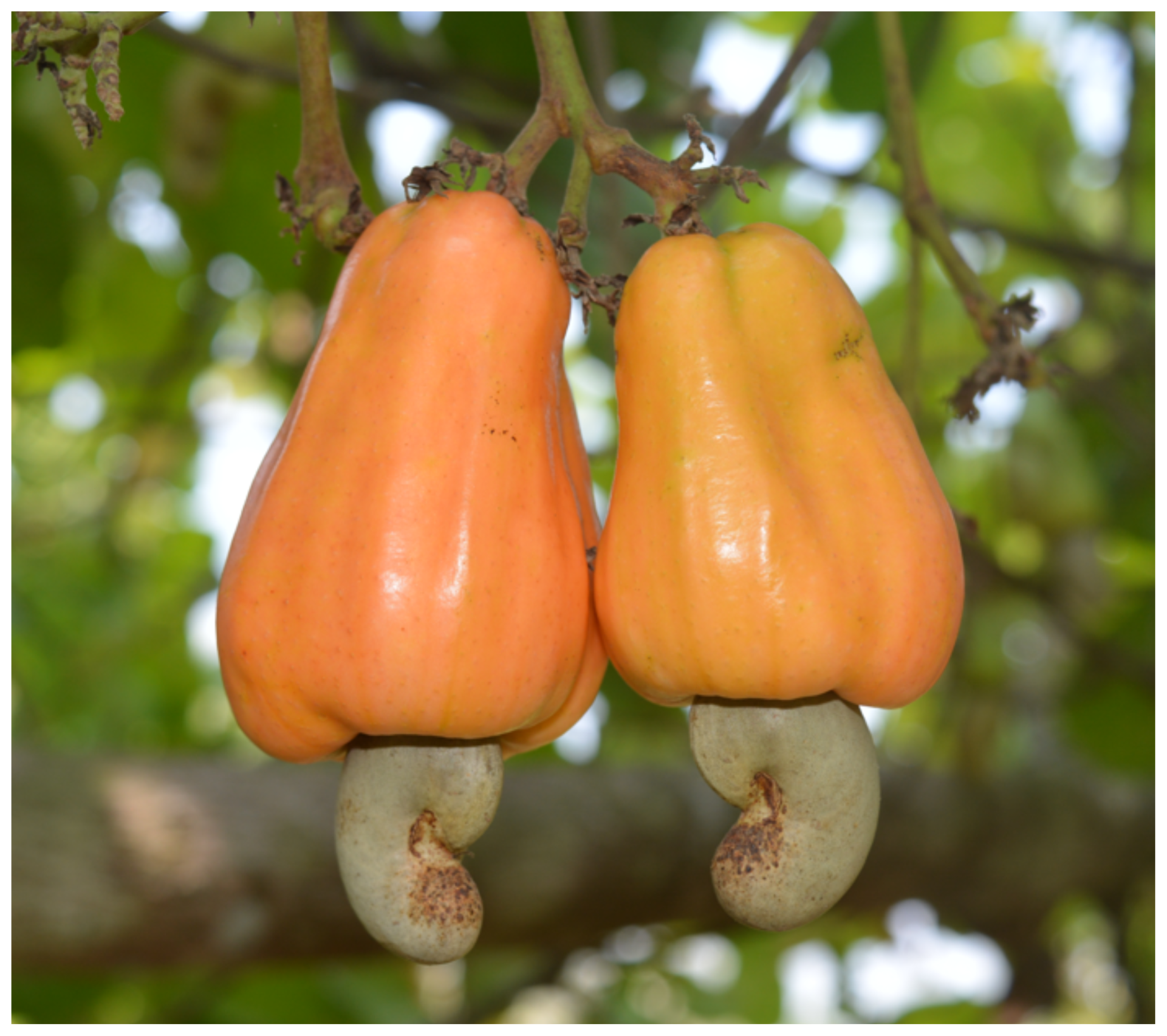
Figure 2.
Flowchart elucidating the research methodology of cashew apple physicochemical properties assessment through computer vision.
Figure 2.
Flowchart elucidating the research methodology of cashew apple physicochemical properties assessment through computer vision.
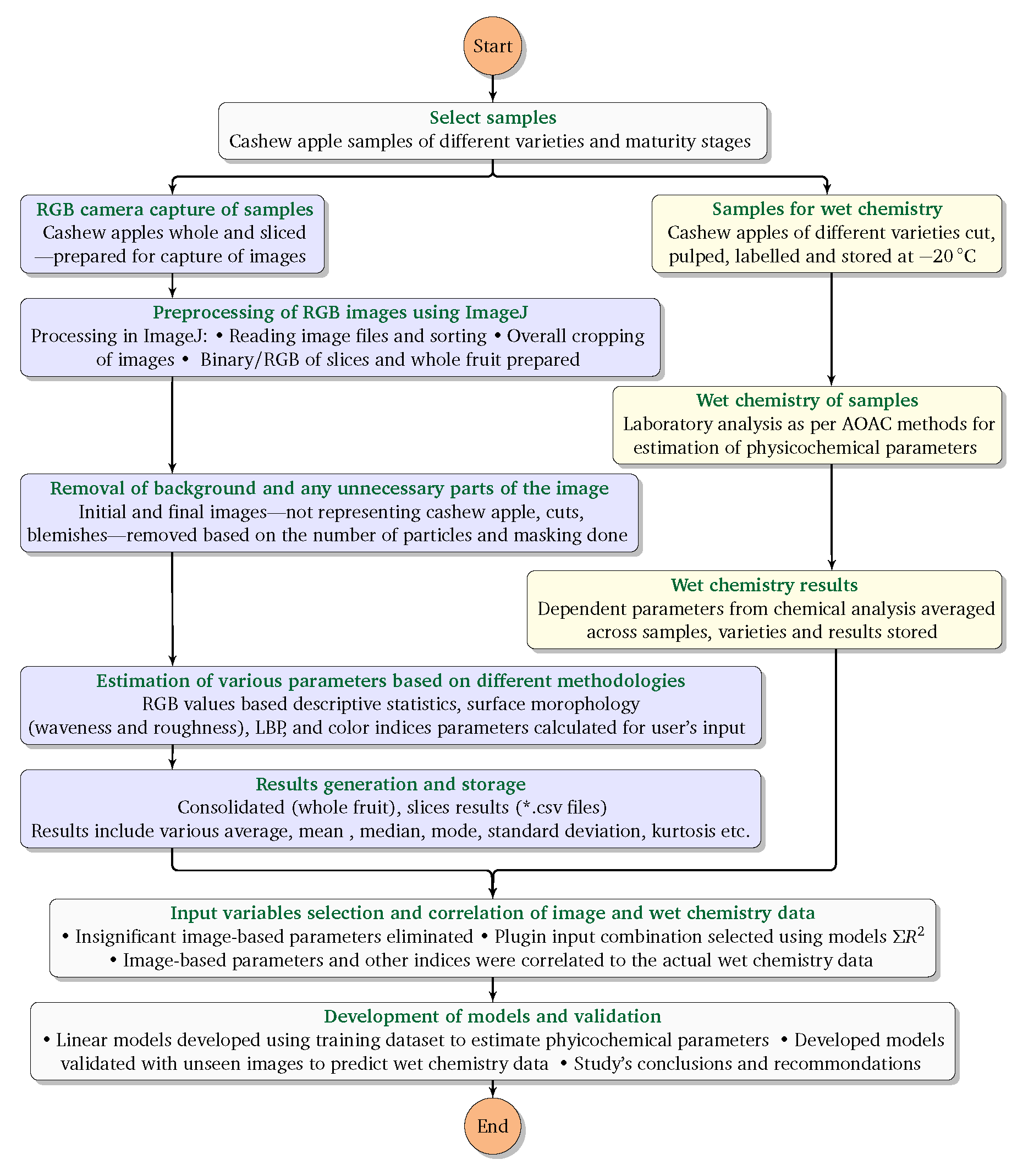
Figure 3.
Six varieties of cashew apples with cut slices, harvested at two stages of maturity. The numbers indicated by 817 and 819 are the two stages of maturity. Complete set of original images is available from the uploaded data [39].
Figure 3.
Six varieties of cashew apples with cut slices, harvested at two stages of maturity. The numbers indicated by 817 and 819 are the two stages of maturity. Complete set of original images is available from the uploaded data [39].
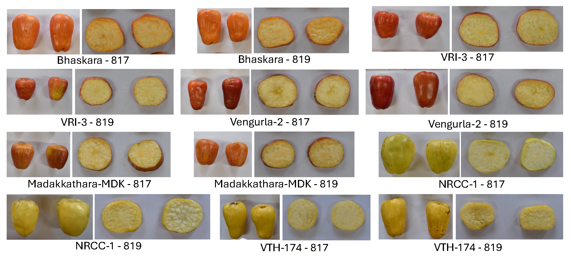
Figure 4.
Various steps followed in the preprocessing of cashew apple slice samples. (A) Collection of samples; (B) cropped individual sample; (C) sample segmentation utilizing ‘U’ channel historam and selection; (D) sample binary image showing unsegmented regions as holes; (E) binary sample image mask after filling holes and median filter; (F) original color image after overlaying with mask; (G) selection of skin areas with polygon tool and smoothening with fit spline; (H) background black filling of selected area; (I) final segmented sample image; (J) cropped whole fruit original image; (K) preprocessed whole fruit showing pedicle cavity and blemishes showing dark spots; and (L) dark regions rectified by pasting similar colored patches giving the final segmented sample image.
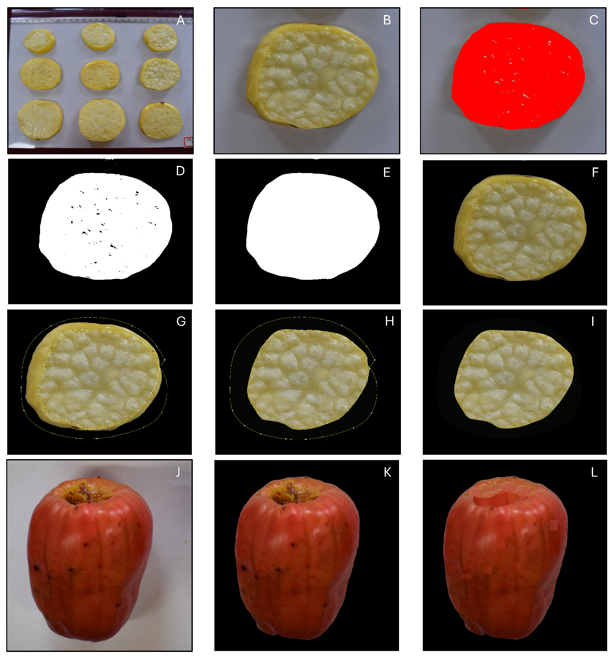
Figure 5.
Processing of images based on different methodologies (A–C). (A1) Preprocessed slice of cashew apple processed in color-based analysis; (A2) ROIs generated for color extraction; (B1) grayscale image for surface morphology analysis; (B2) waveness image with line ROI for sampling; (B3) 3D-waveness surface plot of image; (B4) 3D-roughness surface plot; (B5) roughness mage with line ROI for sampling; (B6) waveness line ROI profile plot; (B7) roughness line ROI profile plot; (C1) grayscale image for LBP; (C2–C4) red, green, and blue component channels, respectively; (C5–C6) texture plots of LBP analysis of gray, red, green, and blue channels; and (D1) analysis progress indicated during batch processing of images.
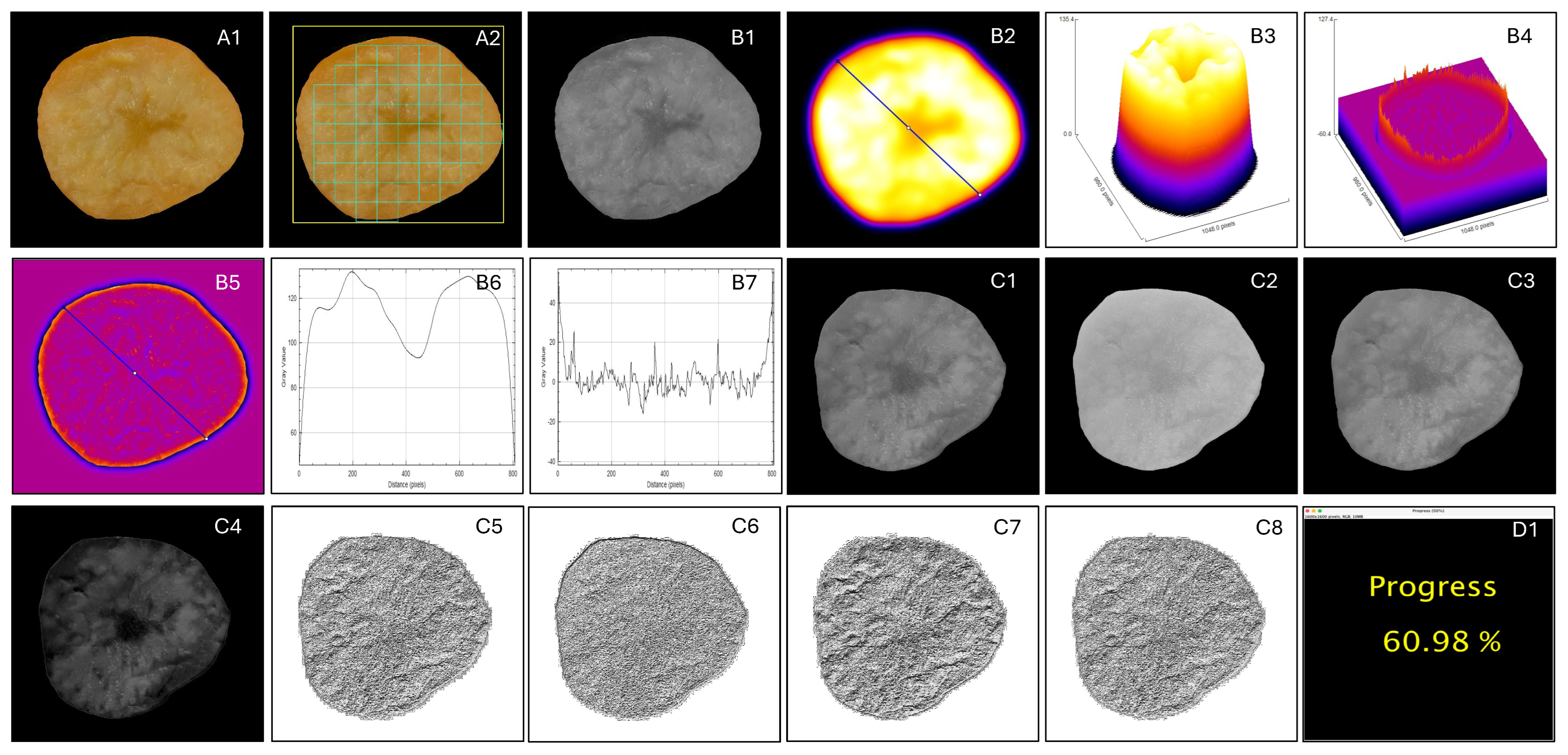
Figure 6.
Input panel of the developed “Cashew Apple and Slices Analysis” batch processing plugin for calculating various image-based parameters used for estimating physicochemical properties of cashew apples. The panel shows brief instructions, various method choices for analysis, input parameters for the methodologies, and buttons to operate the plugin. The main inputs (5 total) are color subimage column and rows (2 inputs), waviness and roughness cutoff pixel (1 input), and GLCM step size pixel and direction degrees (2 inputs).
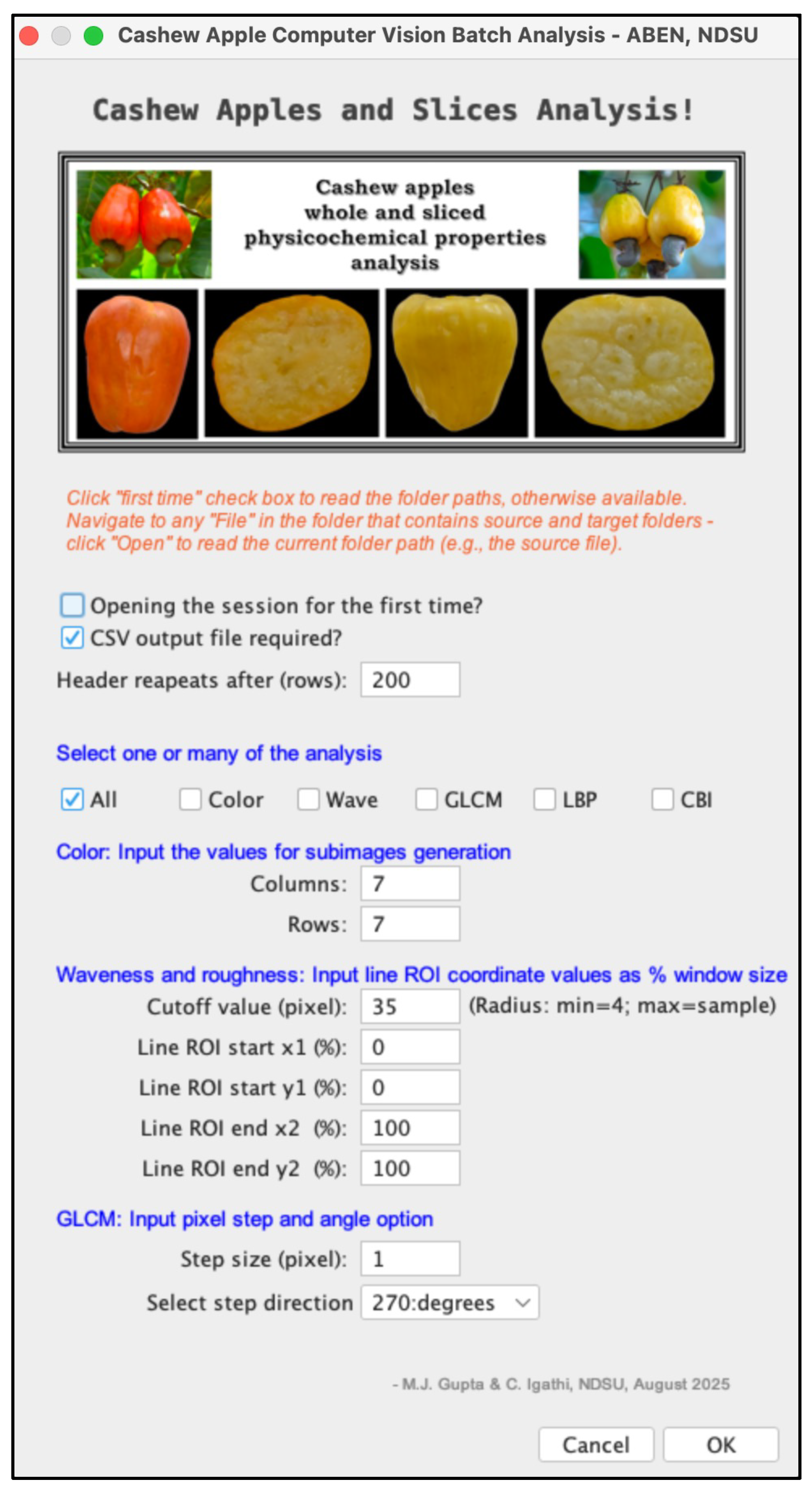
Figure 7.
Correlation diagram for cashew apple sample types demonstrating the correlation of wet chemistry and image-based parameters. Solid horizontal line separates interrelationships among wet chemistry, and dotted horizontal lines separate different parameter groups of methodologies.
Figure 7.
Correlation diagram for cashew apple sample types demonstrating the correlation of wet chemistry and image-based parameters. Solid horizontal line separates interrelationships among wet chemistry, and dotted horizontal lines separate different parameter groups of methodologies.
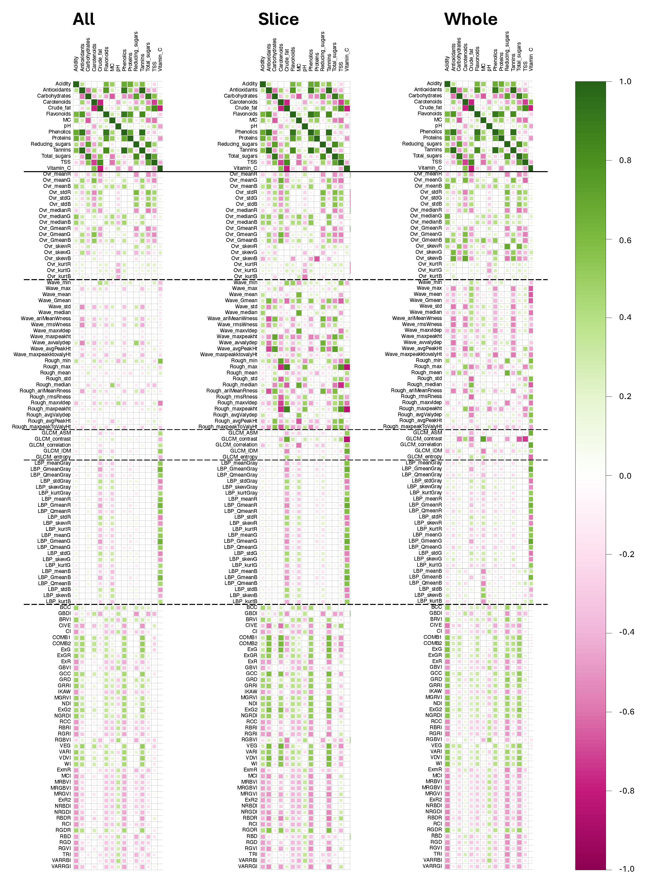
Figure 8.
Range of image-based parameters correlation coefficients with physicochemical properties wet chemistry parameters.
Figure 8.
Range of image-based parameters correlation coefficients with physicochemical properties wet chemistry parameters.
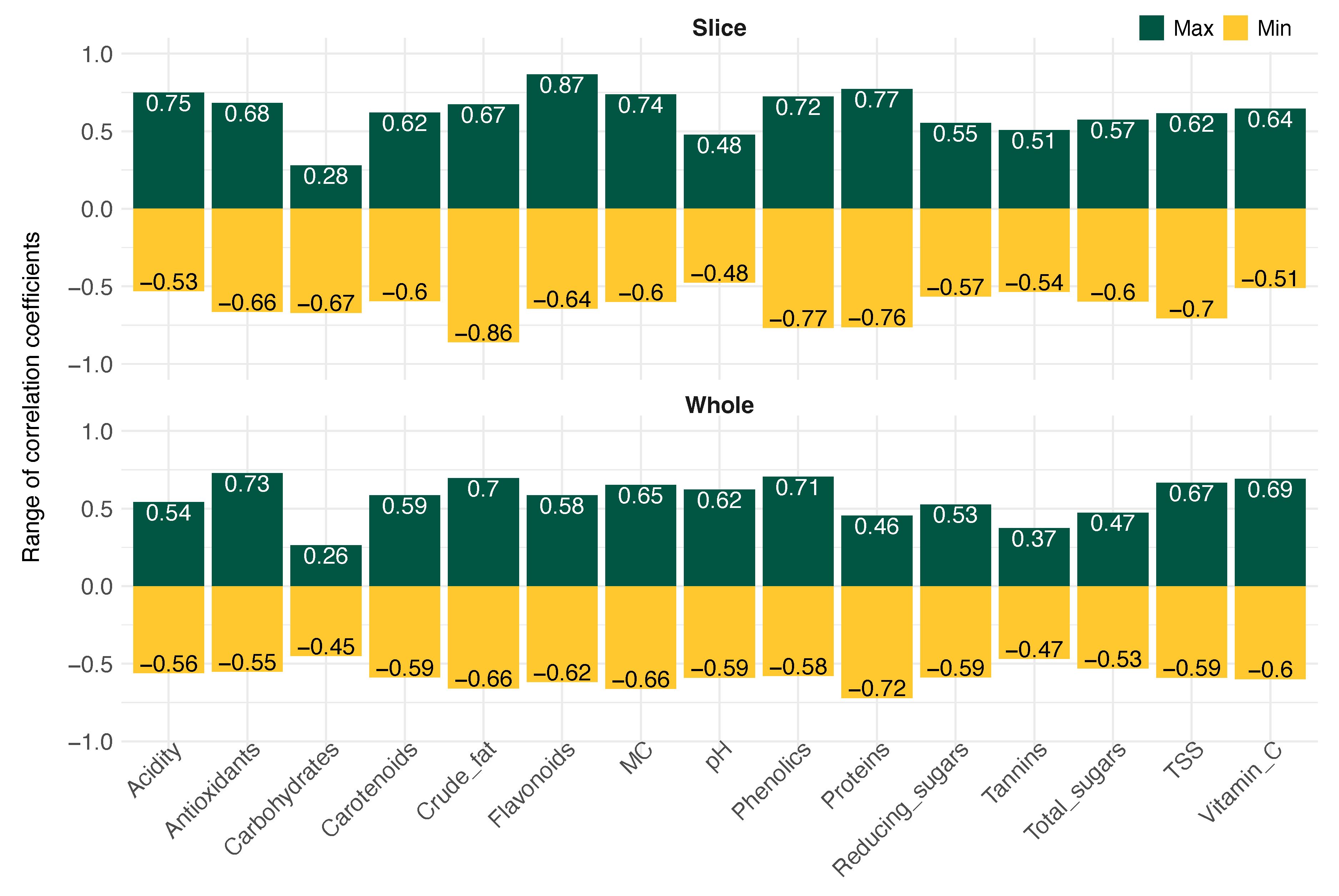
Figure 9.
Prediction and validation showing the ratio change of the predicted to actual physicochemical properties for cashew apple varieties from test image data. The gray dotted horizontal lines across the ratio of 1.0 indicate the ideal prediction.
Figure 9.
Prediction and validation showing the ratio change of the predicted to actual physicochemical properties for cashew apple varieties from test image data. The gray dotted horizontal lines across the ratio of 1.0 indicate the ideal prediction.
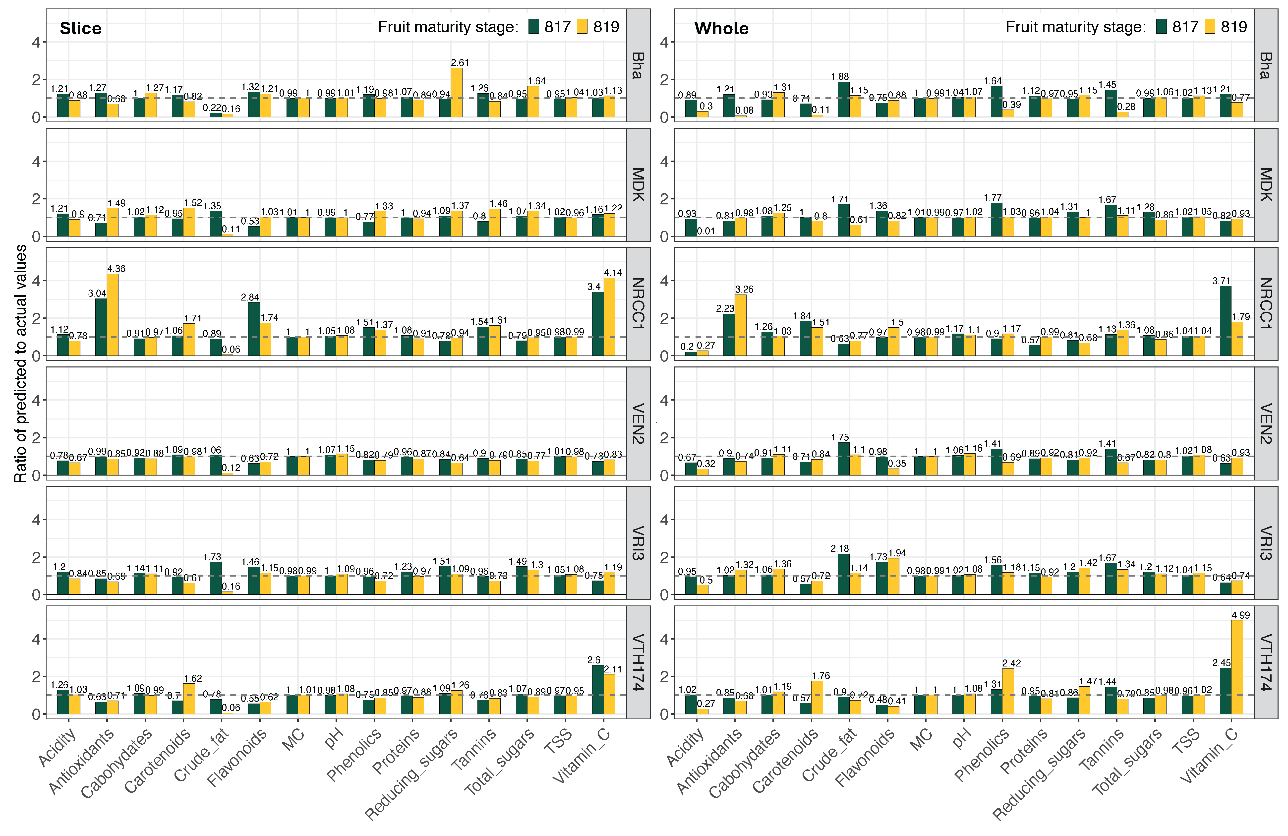

Table 1.
Dependent wet chemistry-based physicochemical properties variables and independent image-based variables employed in the study.
Table 1.
Dependent wet chemistry-based physicochemical properties variables and independent image-based variables employed in the study.
| Methodology | Applicable parameter variables | Total: 159 |
|---|---|---|
| Wet chemistry * | Acidity (titrable), Antioxidant activity, Carbohydrates (total), Carotene (content), Fat crude, Flavonoids (total), Moisture (content), pH, Phenolic (total content), Protein, | |
| Reducing sugars, Tannin (content), Total soluble solids, Total sugars, and Vitamin C (Section 2.2). | Total: 15 | |
| Color grid **,† | Mean R, Mean G, Mean B, Standard deviation of R, Standard deviation of G, Standard deviation of B, Median R, Median G, Median B, Geometric mean R, Geometric | |
| mean G, Geometric mean B, Maximum R, Maximum G, Maximum B, Minimum R, Minimum G, Minimum B, Number of R values, Number of G values, Number of B | ||
| values, Skewness R, Skewness G, Skewness B, Kutosis R, Kutosis G, and Kurtosis B (Section 2.3.3.i). | Total: 27 | |
| Waveness and roughness ** | Descriptive statistics parameters of waveness plot (Number of waveness plot data points, Minimum waveness, Maximum waveness, Mean waveness, Geometric mean | |
| waveness, Standard deviation waveness, Median waveness, Geometric mean waveness, Standard deviation of waveness), Waveness parameters calculated based on | ||
| formulae from references (Arithmetic mean waveness, Root mean square waveness, Maximum valley depth of waveness plot, Maximum peak height of waveness plot, | ||
| Average valley depth of waveness plot, Average peak height of waveness plot, Maximum peak to valley height of waveness plot, Descriptive statistics parameters of | ||
| roughness plot (Number of roughness plot data points, Minimum roughness, Maximum roughness, Mean roughness, Geometric mean roughness, Standard deviation | ||
| roughness, Median roughness), Waveness parameters calculated based on formulas from references (Arithmetic mean roughness, Root mean square roughness, Maximum | ||
| valley depth of roughness plot, Maximum peak height of roughness plot, Average valley depth of roughness plot, Average peak height of roughness curve, and Maximum | ||
| peak to valley height of roughness plot) (Section 2.3.3.ii). | Total: 28 | |
| GLCM ** | Angular second moment, Contrast, Correlation, Inverse difference moment, and Entropy (Section 2.3.3.iii). | Total: 5 |
| LBP **,‡ | Number of gray pixels analyzed, Minimum gray, Maximum gray, Mean gray, Geometric mean gray, Quartile mean gray, Standard deviation gray, Median gray, Skewness | |
| gray, Kurtosis gray, Number of R pixels analyzed, Minimum R, Maximum R, Mean R, Geometric mean R, Quartile mean R, Standard deviation R, Median R, Skewness R, | ||
| Kurtosis R, Number of G pixels analyzed, Minimum G, Maximum G, Mean G, Geometric mean G, Quartile mean G, Standard deviation G, Median G, Skewness G, | ||
| Kurtosis G, Number of B pixels analyzed, Minimum B, Maximum B, Mean B, Geometric mean B, Quartile mean B, Standard deviation B, Median B, Skewness B, and | ||
| Kurtosis B (Section 2.3.3.iv). | Total: 40 | |
| Color indices ** | Color indices derived from overall R, G, and B values (27 existing + 17 new) are given in Table 2. | Total: 44 |
* Dependent variables (total 15); ** Independent variables (total 144); † Overall values derived from the pixels of the selected ROIs based on user inputs; ‡ Set of values analyzed by splitting the color image into the component channels; GLCM - gray level co-occurrence matrix; LBP - local binary pattern; R - red, B - blue, and G - green pixel intensity values.
Table 2.
List of RGB-based indices.
| Vegetation Index | Equation | Reference |
|---|---|---|
| Blue chromatic coordinate (BCC) | [45] | |
| Green-blue difference index (GBDI) | [46] | |
| Blue red vegetation index (BRVI) | [47] | |
| Color index of vegetation (CIVE) | [48,49] | |
| Coloration index (CI) | [50] | |
| Combination1 (COMB1) | [51] | |
| Combination2 (COMB2) | [51] | |
| Excess green (ExG ) | [45,48] | |
| Excess green minus excess red (ExGR) | [48,52] | |
| Excess red (ExR) | [48] | |
| Green-blue vegetation index (GBVI) | [53,54] | |
| Green chromatic coordinate (GCC) | [45] | |
| Green-red difference (GRD) | [46,48] | |
| Green-red ratio index (GRRI) | [48,55] | |
| Kawashima index (IKAW) | [47,48] | |
| Modified green-red vegetation index (MGRVI) | [46,48] | |
| Normalized difference index (NDI) | [56] | |
| Normalized excess green (ExG2) | [45] | |
| Normalized green-red difference index (NGRDI) | [57,58] | |
| Red chromatic coordinate (RCC) | [45] | |
| Red blue ratio index (RBRI) | [59] | |
| Red green ratio index (RGRI) | [60] | |
| Red green blue vegetation index (RGBVI) | [46] | |
| Vegetativen (VEG) | [46] | |
| Visible atmospherically resistant index (VARI) | [61] | |
| Visible-band difference vegetation index (VDVI) | [62] | |
| Woebbecke index (WI) | [45] | |
| Excess modified red (ExmR ) | † | |
| Modified coloration index (MCI) | † | |
| Modified red-blue vegetation index (MRBVI) | † | |
| Modified red-green-blue vegetation index (MRGBVI) | † | |
| Modified red-green vegetation index (MRGVI) | † | |
| Normalized excess red (ExR2) | † | |
| Normalized red-blue difference index (NRBDI) | † | |
| Normalized red-green difference index (NRGDI) | † | |
| Red-blue difference ratio (RBDR) | † | |
| Red color index (RCI) | † | |
| Red-green difference ratio (RGDR) | † | |
| Red-blue difference (RBD) | † | |
| Red-green difference (RGD) | † | |
| Red-green vegetation index (RGVI) | † | |
| Triangular redness index (TRI) | † | |
| Visible atmospherically resistant red-blue index (VARRBI) | † | |
| Visible atmospherically resistant red-green index (VARRGI) | † |
Red (R), blue (B), and green (G) bands recorded from the satellite platforms. * Adopted from GLI. ** Adopted from Triangular greenness index (TGI). † Developed in the present study to capture red-tint-dominated samples.
Table 3.
Cashew apple wet chemistry data for various varieties and maturity stages.
| Wet chemistry | Cashew apple varieties and maturity stages | |||||||||||
|---|---|---|---|---|---|---|---|---|---|---|---|---|
| Bhaskara | MDK | NRCC-1 | Vengurla-2 | VRI-3 | VTH-174 | |||||||
| 817 | 819 | 817 | 819 | 817 | 819 | 817 | 819 | 817 | 819 | 817 | 819 | |
| Acidity (%) | 0.14±0.0 | 0.09±0.01 | 0.12±0.0 | 0.08±0.0 | 0.16±0.0 | 0.12±0.0 | 0.25±0.0 | 0.18±0.0 | 0.16±0.0 | 0.12±0.0 | 0.160±0.0 | 0.11±0.0 |
| Antioxidants (μmol | 28.59±1.13 | 20.85±0.22 | 25.96±0.45 | 8.94±0.11 | 24.39±0.47 | 22.69±0.91 | 26.01±0.83 | 2.88±0.28 | 4.21±0.12 | 11.83±0.87 | 30.47±0.72 | 22.57±0.87 |
| Carbohydrates ( | 14.09±0.93 | 16.35±0.71 | 14.67±0.42 | 17.2±0.69 | 16.94±0.11 | 20.77±0.35 | 16.81±0.24 | 19.24±0.48 | 14.16±1.1 | 15.78±0.41 | 14.67±0.62 | 18.07±0.29 |
| Carotenes (mg | 1.5±0.01 | 1.4±0.01 | 1.41±0.02 | 0.82±0.0 | 1.29±0.0 | 0.34±0.0 | 0.74±0.0 | 1±0.0 | 0.42±0.0 | 0.86±0.0 | 0.57±0.0 | 0.78±0.0 |
| Crude fat (%) | 2.02±0.11 | 1.78±0.04 | 2.73±0.07 | 2.46±0.09 | 5.61±0.04 | 4.59±0.19 | 2.46±0.04 | 2.32±0.04 | 2.23±0.11 | 1.68±0.07 | 5.44±0.01 | 4.66±0.11 |
| Flavonoids (mg | 64.33±13.9 | 106.04±0.0 | 101.49±21.6 | 30.84±2.8 | 25.87±0.4 | 16.78±0.2 | 171.30±56.7 | 71.52±5.7 | 80.24±8.4 | 12.98±3.5 | 218.94±31.8 | 28.47±5.7 |
| MC (% w.b.) | 87.57±0.49 | 85.81±0.56 | 86.42±1 | 85.92±0.8 | 87±0.65 | 85.92±0.32 | 87.31±0.25 | 86±0.21 | 88.89±1.47 | 86.93±0.32 | 86.91±0.28 | 85.26±0.17 |
| pH | 4.56±0.01 | 4.73±0.02 | 4.87±0.02 | 5.23±0.15 | 4.49±0.02 | 4.78±0.01 | 4.29±0.09 | 4.45±0.02 | 4.53±0.01 | 4.69±0.01 | 4.49±0.0 | 4.85±0.04 |
| Phenolics (mg | 311.41±5.1 | 191.77±4.3 | 308.66±6.5 | 134.33±4.0 | 161±7.0 | 124.33±3.8 | 374.7±10.7 | 308.33±6.8 | 318.55±3.5 | 170.49±4.5 | 405.84±4.3 | 243.5±4.8 |
| Proteins (%) | 1.7±0.07 | 1.2±0.04 | 2.16±0.06 | 1.12±0.03 | 2.05±0.07 | 1.18±0.03 | 2.26±0.09 | 1.26±0.04 | 1.78±0.14 | 1.26±0.05 | 2.24±0.09 | 1.45±0.03 |
| Reducing sugars ( | 7.89±0.17 | 6.75±0.38 | 9.33±0.51 | 10.84±0.29 | 14.7±0.59 | 17.68±0.55 | 14.11±0.41 | 16.2±1.34 | 9.04±0.07 | 10.4±0.58 | 12.22±0.71 | 9.7±0.38 |
| Tannins (mg | 2.41±0.11 | 1.65±0.05 | 2.25±0.28 | 0.88±0.03 | 0.91±0.02 | 0.76±0.05 | 2.57±0.07 | 2.36±0.06 | 2.04±0.06 | 1.11±0.03 | 2.53±0.14 | 1.86±0.14 |
| Total sugars ( | 8.62±0.15 | 12.05±0.08 | 10.4±1.27 | 13.07±1.47 | 15.81±0.5 | 19.88±0.6 | 9.92±0.59 | 11.19±0.25 | 15.26±1.26 | 17.81±0.42 | 13.63±0.23 | 17.05±0.26 |
| TSS (°brix) | 2.41±0.11 | 1.65±0.05 | 2.25±0.28 | 0.88±0.03 | 0.91±0.02 | 0.76±0.05 | 2.57±0.07 | 2.36±0.06 | 2.04±0.06 | 1.11±0.03 | 2.53±0.14 | 1.86±0.14 |
| Vitamin C (mg | 98.86±5.1 | 181.71±1.5 | 154.62±3.1 | 252.2±17.4 | 27.5±2.3 | 91.12±0.29 | 197.8±12.3 | 305.5±11.5 | 150.86±2.6 | 305±2.3 | 40.62±2.3 | 69.24±7.6 |
Number of replications employed = 3 and measurement protocols in Appendix A; MC - moisture content; TSS - total soluble solids; and values shown are mean ± 1 standard deviation.
Table 4.
Image analysis input parameters selection based on the sum of based on the top three sets of 180 models.
Table 4.
Image analysis input parameters selection based on the sum of based on the top three sets of 180 models.
| Selected input | Input combination | change from | |
|---|---|---|---|
| *reference (%) | |||
| Waveness cutoff value | ; 4 pix; 1 pix; 0° | 73.900* | 0.00 |
| ; 5 pix; 1 pix; 0° | 73.900 | 0.00 | |
| ; 10 pix; 1 pix; 0° | 75.003 | 1.49 | |
| ; 15 pix; 1 pix; 0° | 75.505 | 2.17 | |
| ; 20 pix; 1 pix; 0° | 75.805 | 2.58 | |
| ; 25 pix; 1 pix; 0° | 75.941 | 2.76 | |
| ; 30 pix; 1 pix; 0° | 76.014 | 2.86 | |
| ; 35 pix***; 1 pix; 0° | 76.043** | 2.90** | |
| ; 40 pix; 1 pix; 0° | 75.966 | 2.80 | |
| ; 50; pix 1 pix; 0° | 75.966 | 2.80 | |
| GCLM step size | ; 35 pix; 1 pix***; 0° | 76.043** | 2.90** |
| ; 35 pix; 2 pix; 0° | 76.023 | 2.87 | |
| ; 35 pix; 3 pix; 0° | 76.024 | 2.87 | |
| ; 35 pix; 5 pix; 0° | 76.031 | 2.88 | |
| ; 35 pix; 10 pix; 0° | 75.933 | 2.75 | |
| GCLM step direction | ; 35 pix; 1 pix; 0° | 76.043 | 2.90 |
| ; 35 pix; 1 pix; 90° | 76.434 | 3.43 | |
| ; 35 pix; 1 pix; 180° | 76.056 | 2.92 | |
| ; 35 pix; 1 pix; 270°*** | 76.437** | 3.43** | |
| Color grid size | ; 35 pix; 1 pix; 270° | 74.670 | 1.04 |
| †***; 35 pix; 1 pix; 270° | 76.437** | 3.43** | |
| ; 35 pix; 1 pix; 270° | 73.751 |
* Reference value from 180 models; ** maximum value at each input block; *** selected combination of image analysis input variables at different evaluation stages; and † final selected input variable combination used for further analysis.
Table 5.
Effect of sample types and analysis groups in correlation analysis of wet chemistry with image-based parameters through absolute and mean Pearson’s correlation coefficient (r and ).
Table 5.
Effect of sample types and analysis groups in correlation analysis of wet chemistry with image-based parameters through absolute and mean Pearson’s correlation coefficient (r and ).
| Parameters group | N | All samples | Slice samples | Whole samples | |||
|---|---|---|---|---|---|---|---|
| Sum | Mean | Sum | Mean | Sum | Mean | ||
| Wet chemistry | 225 | 99.6 | 0.443 | 99.6 | 0.443 | 99.6 | 0.443 |
| Color grid | 270 | 61.0 | 0.226 | 67.8 | 0.251 | 72.2 | 0.267 |
| Waveness and roughness | 375 | 56.7 | 0.151 | 121.6 | 0.324 | 95.1 | 0.254 |
| GLCM | 75 | 9.6 | 0.128 | 16.0 | 0.213 | 17.5 | 0.234 |
| LBP | 360 | 59.3 | 0.165 | 68.2 | 0.189 | 74.0 | 0.206 |
| Color indices | 660 | 156.5 | 0.237 | 193.0 | 0.292 | 179.7 | 0.272 |
| Total image-based | 1740 | 343.1 | 0.197 | 466.5 | 0.268 | 438.6 | 0.252 |
| Total all methods | 1965 | 442.7 | 0.225 | 566.1 | 0.288 | 538.2 | 0.274 |
Data used represent absolute r values with stages (817 and 819) combined; N is the number of parameters in each group; GLCM is gray level co-occurrence matrix; LBP is local binary pattern; Total represents all the combinations of r values of wet chemistry (15) with both wet chemistry and image-based (15 + 116) parameters.
Table 6.
Slice and whole cashew apple top-10 ranking for the wet chemistry properties based on correlation coefficients of image-based independent parameters.
Table 6.
Slice and whole cashew apple top-10 ranking for the wet chemistry properties based on correlation coefficients of image-based independent parameters.
| Wet chemistry | Ranks of image-based independent variables based on correlation (r) values | |||||||||
|---|---|---|---|---|---|---|---|---|---|---|
| properties | 1 | 2 | 3 | 4 | 5 | 6 | 7 | 8 | 9 | 10 |
| Slice | ||||||||||
| Acidity | Wn-avPH | Wn-mxPH | Wn-amWn | Rn-amRn | Rn-xpvh | Rn-avPH | Rn-med | Wn-Gmn | Ov-stdR | Rn-mxVD |
| Antioxidants | Rn-med | Wn-med | Rn-avPH | Wn-mxVD | Wn-mn | Gl-corr | Rn-avVD | Wn-Gmn | Ov-medG | Wn-mxPH |
| Carbohydrates | Ov-skB | Wn-xPt | Rn-mn | Rn-avPH | Rn-xpvh | Wn-med | Gl-corr | Gl-cont | Rn-avVD | Wn-avPH |
| Carotenes | VDVI | GCC | ExG2 | VEG | COMB1 | COMB2 | ExG | CIVE | RGDR | Wn-avPH |
| Crude fat | Gl-cont | Rn-mxPHt | Rn-mx | L-GmnR | L-GmnG | L-GmnGr | Gl-IDM | L-GmnB | Rn-mi | Rn-mxVD |
| Flavonoids | Rn-mxPH | Rn-mx | Gl-cont | Rn-med | Wn-Gmn | L-GmnR | Gl-IDM | RGBVI | Rn-mi | L-GmnG |
| MC | Wn-avPH | Wn-mxPH | Rn-med | Wn-amWn | Rn-amRn | Ov-stdR | Ov-stdB | Rn-xpvh | Ov-medR | Ov-GmnG |
| pH | Wn-med | GRD | RGD | Ov-medG | RBRI | ExmR | TRI | RCC | ExR2 | BRVI |
| Phenolics | Rn-mx | Rn-mxPH | Rn-mi | Rn-mxVD | Ov-mnG | Rn-xpvh | Rn-amRn | Rn-std | VEG | Ov-GmnG |
| Proteins | Rn-mx | Rn-mxPH | Rn-med | Wn-Gmn | Ov-mnG | Rn-avPH | Wn-mxVD | Ov-GmnG | Rn-xpvh | Wn-mi |
| Reducing sugars | Wn-avPH | Wn-mxPH | Wn-Gmn | Ov-medB | Rn-xpvh | ExGR | Ov-medG | VARI | VARRGI | RGRI |
| Tannins | Wn-avPH | Wn-mxPH | Wn-mi | Rn-xpvh | Wn-amWn | Rn-amRn | Ov-skB | Wn-rsWn | Wn-std | Wn-Gmn |
| Total Sugars | Ov-medG | RBRI | BRVI | IKAW | NRBDI | BCC | CI | MRBVI | MRGBVI | RCC |
| TSS | Wn-avPH | Wn-amWn | Rn-amRn | Wn-Gmn | VEG | VDVI | GCC | ExG2 | COMB1 | COMB2 |
| Vitamin C | Wn-avVD | Wn-amWn | Rn-amRn | Ov-stdR | Wn-avPH | Ov-GmnR | Wn-rsWn | Wn-std | Ov-mnR | Ov-stdB |
| Whole | ||||||||||
| Acidity | Gl-cont | Ov-skR | Ov-skG | Ov-skB | Rn-mn | Ov-medR | Ov-stdR | Ov-stdB | VEG | GCC |
| Antioxidants | Gl-cont | Ov-GmnB | Gl-IDM | L-QmnB | L-mnB | L-skB | L-kuB | L-stdB | Wn-avVD | RGBVI |
| Carbohydrates | Rn-mxPH | Rn-mx | Gl-IDM | Wn-mi | Wn-mxVD | Wn-avVD | Wn-amWn | Rn-amRn | L-GmnG | L-GmnGr |
| Carotenes | Wn-xpvh | Ov-mnG | Ov-skB | Wn-rsWn | Wn-std | Ov-GmnB | Wn-amWn | Rn-amRn | Wn-mx | Wn-avVD |
| Crude fat | L-GmnG | L-GmnGr | Gl-corr | Rn-med | Wn-mn | Wn-mx | Wn-Gmn | Gl-ASM | L-GmnR | L-GmnB |
| Flavonoids | Rn-rsRn | Rn-std | Rn-med | Rn-mxPH | Rn-mx | Rn-avVD | Gl-cont | Ov-medR | Wn-avPH | Wn-mn |
| MC | Gl-cont | Ov-skR | Ov-medR | Ov-stdB | Ov-stdR | Ov-GmnR | Ov-mnR | GCC | ExG2 | VDVI |
| pH | Ov-medG | Ov-mnB | CIVE | ExG | Ov-GmnB | WI | RBDR | COMB1 | COMB2 | RGDR |
| Phenolics | Ov-skB | Ov-mnG | Ov-GmnG | Wn-avPH | Ov-GmnB | Ov-stdR | Wn-rsWn | Wn-std | Wn-amWn | Rn-amRn |
| Proteins | Gl-cont | Ov-mnG | Ov-GmnG | Ov-GmnB | Rn-mxPH | Rn-mx | Ovr-medR | Rn-avVD | Rn-std | Rn-rsRn |
| Reducing sugars | Wn-xpvh | Ov-GmnB | Wn-mxVD | Wn-mx | Ov-skG | Ov-mnG | Ov-mnB | CIVE | ExG | Wn-rsWn |
| Tannins | Wn-xpvh | Rn-mx | Rn-mxPH | Wn-mxVD | Ov-GmnB | Wn-mx | Ov-medB | CIVE | Ov-mnB | ExG |
| Total Sugars | Ov-GmnB | Ov-mnB | CIVE | ExG | L-kuB | Ov-medG | COMB2 | COMB1 | L-skB | VDVI |
| TSS | Ov-skB | Ov-skG | Wn-xpvh | Wn-rsWn | Wn-std | Wn-avVD | Wn-amWn | Rn-amRn | Ov-mnG | Wn-mx |
| Vitamin C | Ov-skR | Rn-mn | Ov-stdR | Ov-skB | Rn-mi | Rn-mxVD | Ov-GmnR | Ov-mnR | Ov-medR | Ov-stdB |
Short forms for the image-based independent parameters were used. They can be combined to make the complete image-based independent property names. Table 1 list the full form. Short forms utilized are: am - arithmetic mean, av - average, B - blue, cont - contrast, corr - correlation, G - green, Gl - gray level co-occurrence matrix, Gmn - geometric mean, Gr - gray, IDM - inverse difference moment, kurt - kurtosis, L - local binary pattern, med - median, mi - minimum, mx - maximum, Ov - overall, PH - peak height, pvh - peak to valley height, rs - root mean square, R - red, Rn - roughness. sk - skewness, std - standard deviation, VD - valley depth, and Wn - waveness; color-based indices: BCC, CIVE, COMB1, COMB2, ExG, ExG2, GCC, GRD, MRGBVI, RBDR, RGD, RGDR, RGBVI, VDVI, VEG, and WI are available from Table 2; MC - moisture content; and TSS - total soluble solids.
Table 7.
Cashew apple slice and whole top-three ranked linear models of wet chemistry parameters with image-based parameters as independent variables from the training image dataset.
Table 7.
Cashew apple slice and whole top-three ranked linear models of wet chemistry parameters with image-based parameters as independent variables from the training image dataset.
| Wet chem. (y) | x | Model () | x | Model () | Wet chem. (y) | x | Model () | x | Model () |
|---|---|---|---|---|---|---|---|---|---|
| Slice | |||||||||
| Stage = 817 | Stage = 819 | Stage = 817 | Stage = 819 | ||||||
| Acidity | Ov-medR | WI | Antioxidant | VDVI | VEG | ||||
| Ov-mnR | RBDR | GCC | Ov-mnG | ||||||
| Ov-GmnR | Ov-medG | ExG2 | COMB2 | ||||||
| Carbohydrates | Ov-stdR | Ov-skG | Carotenoids | VEG | Rn-xpH | ||||
| Ov-GmnB | Ov-kuB | COMB1 | Rn-mx | ||||||
| Ov-stdB | Ov-stdR | COMB2 | Rn-mpvh | ||||||
| Crude fat | VEG | Gl-cont | Flavonoids | ExmR | VEG | ||||
| COMB2 | Rn-mx | TRI | COMB2 | ||||||
| COMB1 | Rn-xpH | RBD | COMB1 | ||||||
| MC | Ov-kuB | Rn-mx | pH | RBD | Ov-GmnB | ||||
| RBD | Rn-mxPH | TRI | CIVE | ||||||
| TRI | Rn-mpvh | ExmR | ExG | ||||||
| Phenolics | GRD | VEG | Proteins | Ov-GmnB | Ov-kuR | ||||
| RGD | COMB2 | Ov-stdB | Ov-kuG | ||||||
| ExmR | COMB1 | Ov-mnB | Ov-medR | ||||||
| R-sugars | Ov-stdR | Ov-skG | Tannins | VDVI | VEG | ||||
| Ov-stdB | Ov-stdR | GCC | COMB2 | ||||||
| Ov-GmnG | Ov-stdB | ExG2 | COMB1 | ||||||
| T-sugars | Ov-stdR | Ov-skG | TSS | VEG | Rn-mx | ||||
| Ov-stdB | Ov-medR | COMB1 | Rn-mxPH | ||||||
| Ov-GmnG | Ov-stdB | COMB2 | Rn-mpvh | ||||||
| Vitamin C | L-GmnR | Rn-mpvh | |||||||
| L-GmnGr | Rn-mx | ||||||||
| L-GmnB | Rn-mxPH | ||||||||
| Whole | |||||||||
| Stage = 817 | Stage = 819 | Stage = 817 | Stage = 819 | ||||||
| Acidity | WI | Ov-medG | Antioxidant | Ov-skG | Ov-skG | ||||
| RBDR | Ov-GmnB | Wn-mxPH | Wn-avVD | ||||||
| RGDR | Ov-mnB | Wn-mx | Wn-mxVD | ||||||
| Carbohydrates | Ov-skG | Gl-cont | Carotenoids | Ov-GmnG | Ov-skG | ||||
| Ov-kuB | COMB1 | Ov-stdR | Wn-mxVD | ||||||
| Ov-stdR | COMB2 | Ov-stdG | Wn-xpvh | ||||||
| Crude fat | Ov-mnG | VEG | Flavonoids | Wn-xpvh | Ov-kuB | ||||
| Ov-GmnG | L-GmnG | Ov-kuR | VEG | ||||||
| Gl-cont | L-GmnGr | WI | Wn-med | ||||||
| MC | Gl-cont | RGBVI | pH | WI | Ov-GmnB | ||||
| Ov-kuB | Gl-cont | RBDR | Ov-medG | ||||||
| Ov-medG | Ov-GmnB | RGDR | Ov-mnB | ||||||
| Phenolics | Wn-mx | Ov-skG | Proteins | Gl-cont | Ov-kuB | ||||
| Wn-xpvh | Ov-kuB | Ov-stdR | Ov-kuR | ||||||
| Ov-kuR | Wn-mxVD | Ov-stdB | WI | ||||||
| R-sugars | Ov-skG | Ov-stdR | Tannins | Wn-mx | Ov-skG | ||||
| Ov-stdR | RBRI | Wn-mxPH | Wn-avVD | ||||||
| Ov-medR | Ov-medG | Ov-mnG | Wn-mxVD | ||||||
| T-sugars | Ov-skG | VEG | TSS | Gl-cont | Gl-cont | ||||
| Ov-stdR | COMB1 | Ov-mnG | Ov-skG | ||||||
| Ov-medR | COMB2 | Ov-GmnG | Ov-medR | ||||||
| Vitamin C | Rn-avVD | Wn-Gmn | |||||||
| Wn-mn | Wn-mn | ||||||||
| Wn-Gmn | Wn-mxVD | ||||||||
Short forms for the image-based independent parameters were used. They are combined to make the image-based independent properties, hence refer Table 1 to obtain the full form. Short forms: am - arithmetic mean, av - average, B - blue, cont - contrast, corr - correlation, G - green, Gl - gray level co-occurrence matrix, Gmn - geometric mean, Gr - gray, IDM - inverse difference moment, kurt - kurtosis, L - local binary pattern, med - median, mi - minimum, mx - maximum, Ov - overall, PH - peak height, pvh - peak to valley height, rs - root mean square, R - red, Rn - roughness. sk - skewness, std - standard deviation, VD - valley depth, and Wn - waveness; color-based indices: CIVE, COMB1, COMB2, ExG, ExG2, GBVI, GCC, GRD, RBD, RBDR, RGD, RGDR, RGBVI, VDVI, VEG, and WI are available from Table 2; MC - moisture content; and TSS - total soluble solids.
Disclaimer/Publisher’s Note: The statements, opinions and data contained in all publications are solely those of the individual author(s) and contributor(s) and not of MDPI and/or the editor(s). MDPI and/or the editor(s) disclaim responsibility for any injury to people or property resulting from any ideas, methods, instructions or products referred to in the content. |
© 2025 by the authors. Licensee MDPI, Basel, Switzerland. This article is an open access article distributed under the terms and conditions of the Creative Commons Attribution (CC BY) license (http://creativecommons.org/licenses/by/4.0/).
Copyright: This open access article is published under a Creative Commons CC BY 4.0 license, which permit the free download, distribution, and reuse, provided that the author and preprint are cited in any reuse.


