
Submitted:
10 October 2025
Posted:
11 October 2025
You are already at the latest version
Abstract
For small to medium-sized fruits, such as cherries and blueberries, phenotypic data such as fruit size and various diameters are key indicators for fruit breeding, providing essential references for the breeding process. Currently, manual measurements that are widely used are inefficient and introduce significant uncertainties. To address this, this study designed breeding equipment that leveraged machine vision technology to capture fruit images and perform size measurements and evaluations using LabVIEW programming. Using cherries as an example, the RGB images were converted to grayscale using a weighted average method, followed by flat-field correction to remove artifacts and noise. The Canny algorithm was then applied to extract the fruit contour, and the Otsu algorithm was employed for automatic thresholding in the image binarization. Morphological processing separated the fruit from the stem, and template-matching technology was used to define the region of interest (ROI) for measurement. The system achieved an average relative error of only 0.35%, with a standard deviation of 0.0828 and a measurement time of 2.547 s per cherry. This method significantly improved the efficiency and saved time compared to traditional manual measurements. The device successfully measured fruits such as cherries and blueberries, providing a new tool for fruit size measurement in the breeding process and offering valuable insights for the design of future equipment.
Keywords:
breeding equipment
; machine vision
; non-contact measurement
; non-destructive testing
1. Introduction
Fruit size plays a crucial role in the breeding of small-fruit tree varieties such as cherries, blueberries, apricots, and plums. In such fruit tree breeding, breeders have traditionally prioritized the development of large fruit varieties, owing to the direct impact of fruit size on market value and consumer demand. To accurately assess fruit size, breeders focus on key parameters, such as single fruit weight, fruit length, and fruit diameter, which not only provide a clear indication of fruit volume but also reflect its appearance and quality to some extent.
The current assessment of the longitudinal and transverse diameters of these fruits relies primarily on manual measurement methods. Given the short shelf life of fruits and the large number of breeding materials, there is an urgent need to measure a significant number of samples in a limited time. However, this process requires substantial human resources, and the results are prone to considerable uncertainty. Manual measurement is not only time-consuming and labor-intensive but also susceptible to human error, leading to inconsistent and inaccurate results. Furthermore, the varying shapes and sizes of fruits reduce the efficiency of manual measurement, particularly when handling large sample sizes, making manual methods inadequate for the demands of modern agricultural breeding.
There is an urgent need to develop an efficient and accurate automated measurement method to replace traditional manual techniques. To address this, machine-vision-based technology can be employed to capture fruit images for precise size measurements. Currently, machine vision is widely used in breeding and phenotyping, enabling high-throughput analysis of fruits [1,2,3,4,5], seeds [6,7,8,9,10], and overall plant health [11,12].For instance, For instance, Falk et al. [13] developed a computer vision and machine learning pipeline for soybean root phenotyping, demonstrating the potential of automated image analysis in plant breeding research. Wu et al. [2] utilized machine vision technology to extract the phenotypic characteristics of Perilla seeds with different vigor levels and identified rapid seed vigor detection indicators through correlation analysis, thereby reducing early stage detection costs. Similarly, Nadia Ansari et al. [3] integrated machine vision with multivariate analysis methods to develop a rapid classification and detection method for rice seeds based on variety purity. Zhu [14] proposed a method to obtain corn phenotypic parameters by processing images of corn ears and kernels, achieving a 97.6% success rate in precisely segmenting overlapping corn in the collected images. Li [6] applied machine vision technology to integrate an algorithm for acquiring the phenotypic traits of soybean seeds into the control system of a seed selection device, significantly reducing manual errors and greatly improving seed selection efficiency. However, no specialized image acquisition and size measurement equipment has yet been developed for small fruits such as cherries, blueberries, apricots, and plums.Therefore, this study proposed a size measurement system utilizing the machine vision technology for non-contact, precise measurements. Compared with traditional manual methods, this system significantly improved the measurement efficiency, reduced the time costs, and produced results with less numerical fluctuation.
2. Materials and Methods
2.1. Materials and Procedure
In this experiment, using cherries as an example, a 500 W pixel distortion-free industrial camera was employed to capture images. Cherry samples of the Meizao variety were provided by the Shandong Institute of Pomology. The program was developed in the LabVIEW environment with vision functions implemented through Vision and Machine modules. Before conducting the size measurements, image processing operations such as flat-field correction, morphological processing, calibration, and matching were performed.
2.2. Preliminary Image Processing
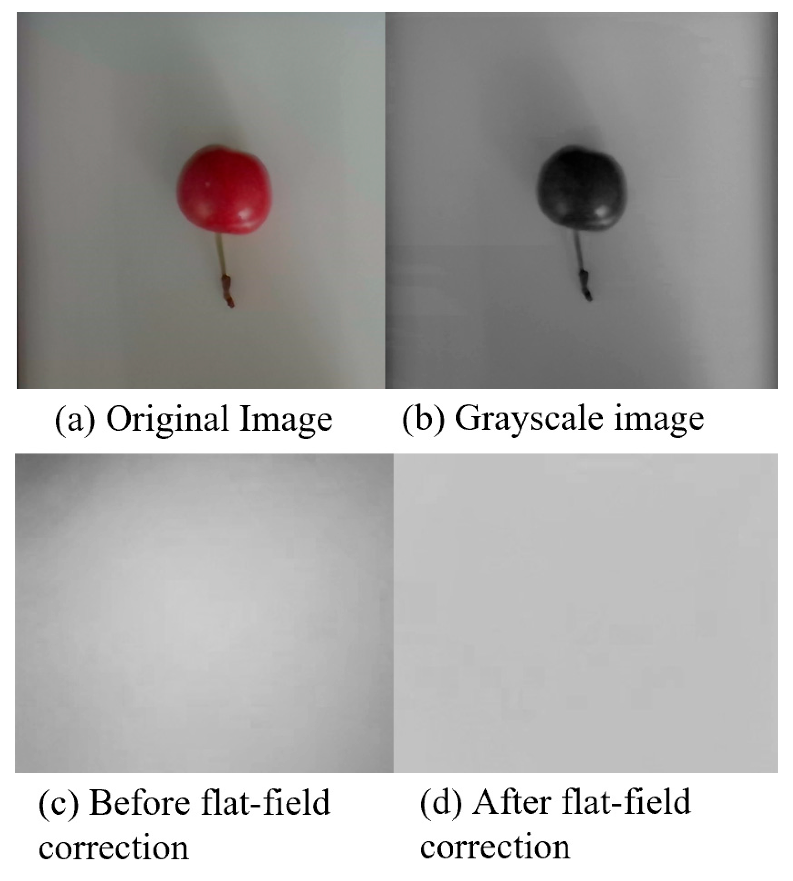
The system captured images using a 500 W pixel distortion-free industrial camera, utilizing backlighting as the light source. Similar camera configurations have been successfully applied in measuring morphological features of radiata pine seedlings [18], confirming the suitability of this hardware selection for plant phenotyping applications. After capturing the cherry images, grayscale processing was applied, as the captured RGB images, where each pixel consisted of three RGB channels, contained excessive color information that was not crucial and would slow the computational speed of the computer. The images were first converted to grayscale as grayscale processing filters out color information, reducing the image to a single channel that only provides brightness information, thereby decreasing the processing time. To retain key information while excluding unnecessary data, the device employed the weighted average method, which assigned different weights to three components based on their importance. Because human eyes were the most sensitive to green and least sensitive to blue, a reasonably accurate grayscale image was obtained using a formula that accounts for this color sensitivity.
Owing to interference factors such as lighting differences, the brightness and color across the image were not uniform. To achieve more uniform brightness across different regions and minimize the impact of artifacts, noise, and other factors, flat-field correction was applied to the image.
Figure 1.
Effect diagrams of grayscale processing and flat-field correction.
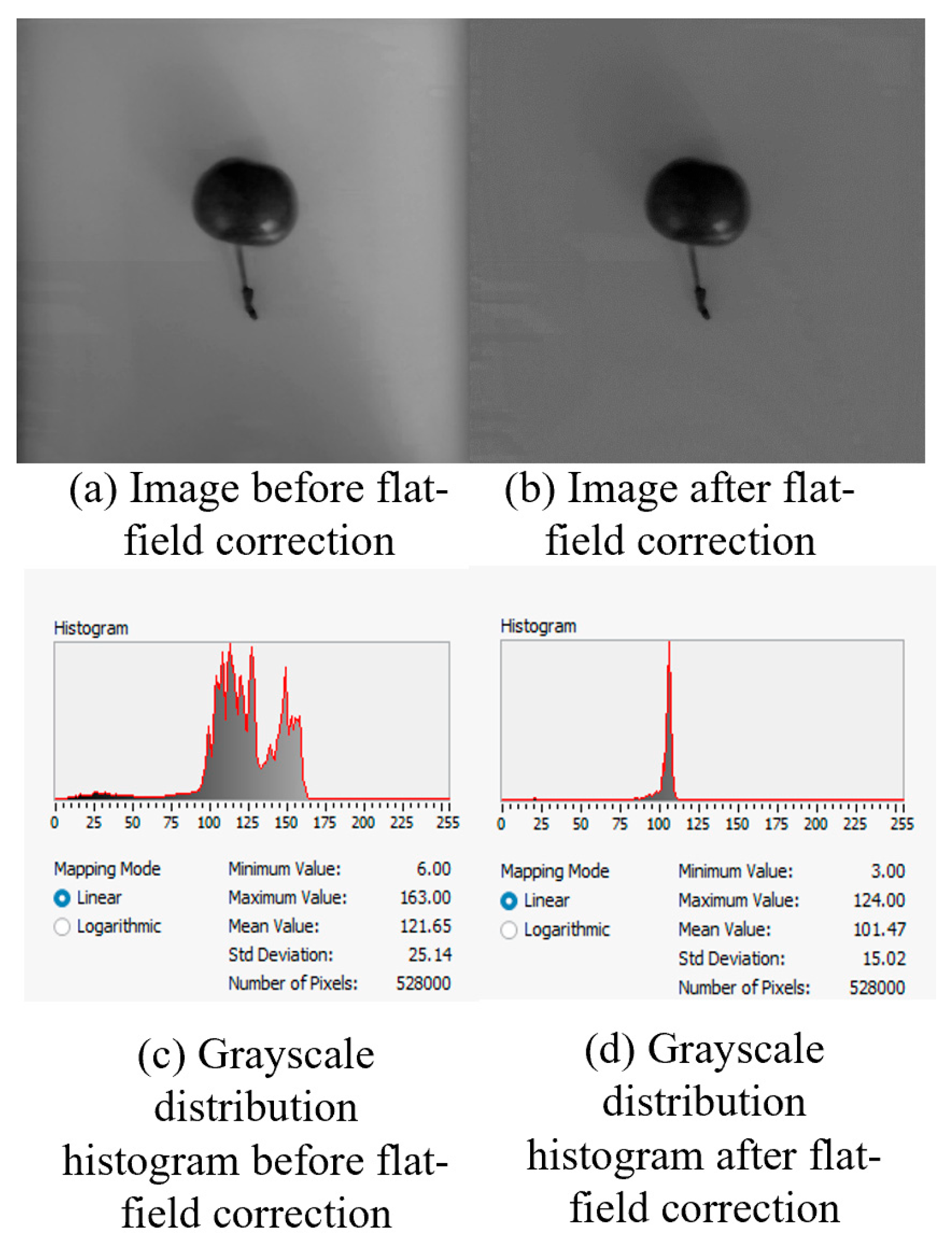
The flat-field correction consisted of photo response nonuniformity (PRNU) correction and dark signal nonuniformity (DSNU) correction. The PRNU correction, or bright-field correction, requires capturing a reference image under uniform lighting conditions, denoted as F. DSNU correction, or dark-field correction, involves capturing an image in complete darkness, where the dark-field image represents the noise generated by the camera without any light signal, denoted as D. The pixel-wise calculation of the image matrix is expressed as follows:
After processing, is the normalized image. The mean value of the difference between the bright-field and dark-field images was utilized as the magnification factor to adjust the normalized image back to the grayscale range of 0–255. The formula for calculating the magnification factor is as follows:
where N denotes the number of pixels in the image. Based on the above formulas, the correction process is as follows:
Analysis of the grayscale histogram before and after flat-field correction following a linear mapping pattern revealed that the standard deviation of the grayscale values decreased from 25.14 before processing to 15.02 after correction. The curve clearly illustrates that the grayscale values were more concentrated than before, the image became more uniform, and the impact of lighting differences on the image was significantly improved.
Figure 2.
Images before and after flat-field processing and related grayscale histograms.
2.3. Edge Contour Detection
To identify the most suitable edge detection algorithm for this experiment, the commonly used algorithms Canny, Sobel, and Roberts were tested to determine the optimal choice.
A circular image was used as the original image. To simulate an actual detection environment, a 5×5 convolution kernel was applied to create a blurred version. Contours were then extracted from the blurred images using the Canny, Sobel, and Roberts algorithms. The maximum contour distance in eight directions was measured for each contour-extracted image, and the results are shown in Figure 3.
The measurement results indicated that for the original image, the number of farthest pixels on its edge ranged between 379.22 and 380.36 across different directions. However, after blurring the image, the edges became difficult to determine, and the contours extracted using the Canny, Sobel, and Roberts algorithms exhibited varying degrees of deviation. The Canny algorithm proved significantly more accurate in matching the actual contours, thereby providing more precise measurement results. Consequently, the Canny algorithm was selected for contour extraction in this study.
Figure 4.
Related image processing and effect diagrams.
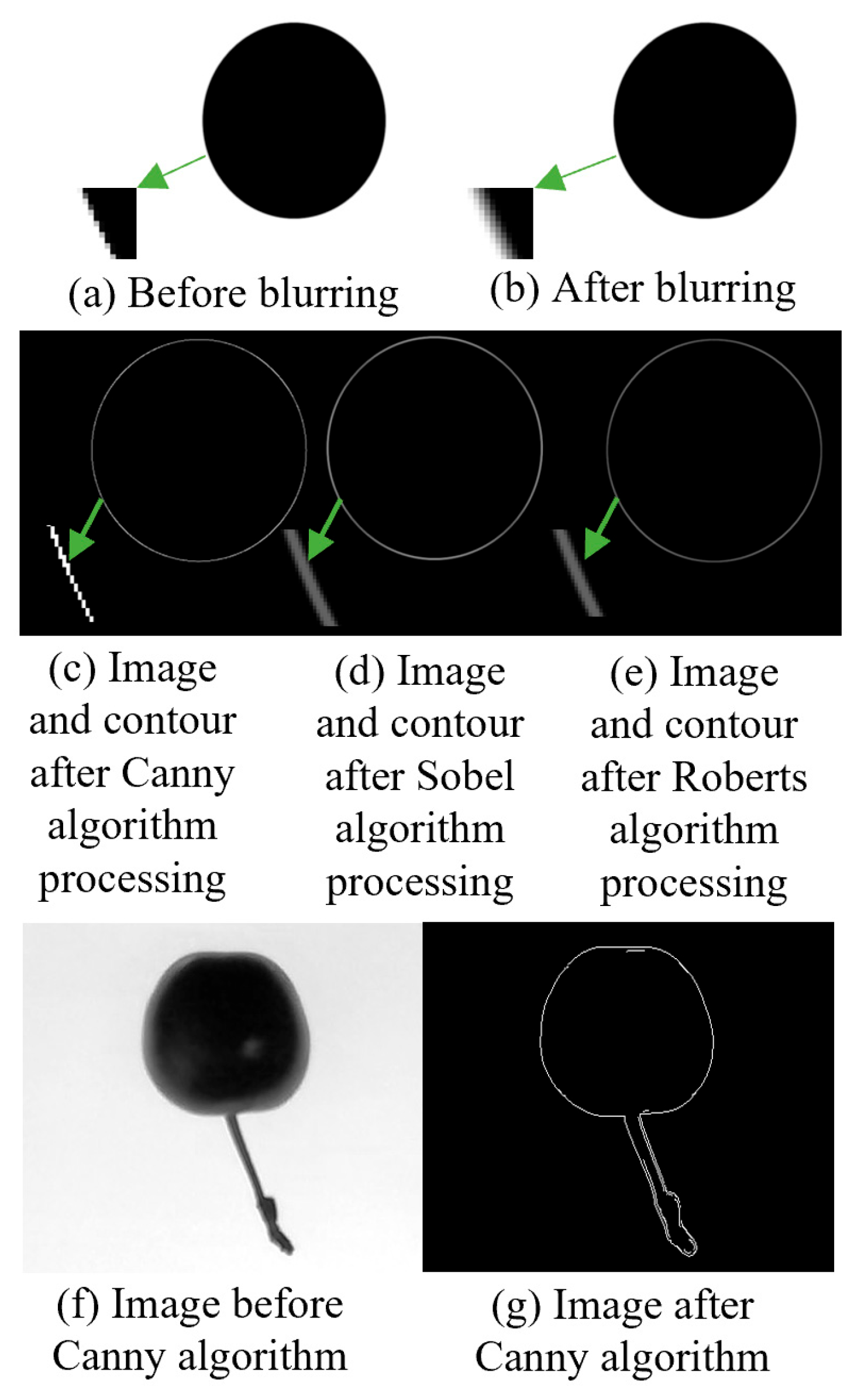
To facilitate subsequent stem separation and remove unnecessary curves after applying the Canny algorithm, the Otsu algorithm was applied to automatically threshold and binarize the image, thereby enhancing the speed of image processing.
2.4. Morphological Processing
Common morphological processing methods include dilation, erosion, closing, and opening.
(1) Dilation (Dilate)
In the dilation operation, the size of the brighter objects in the image increases, whereas the size of the darker objects decreases. For two sets A and B, this relationship is expressed using the following formula:
where is the translation of set B; and is the mapping of set B.
(2) Erosion (Erode)
Erosion is an operation that identifies the local minimum, reducing and thinning the bright or white regions in an image, causing the bright regions in the processed image to become smaller than those in the original image. This process is expressed as follows:
(3) Closing (Close)
Closing is an operation consisting of dilation followed by erosion, which smoothens the contours, fills the holes within the target, eliminates small black holes, and bridges narrow breaks and thin gaps, thereby providing an overall smoothing effect. This is represented by the following equation:
(4) Opening (Open)
The opening operation smoothing the contours is the reverse of closing and consists of erosion followed by dilation. It breaks the narrow connections, removes isolated small points outside the target features, and eliminates small protrusions or burrs on the contour lines. This is represented by the following equation:
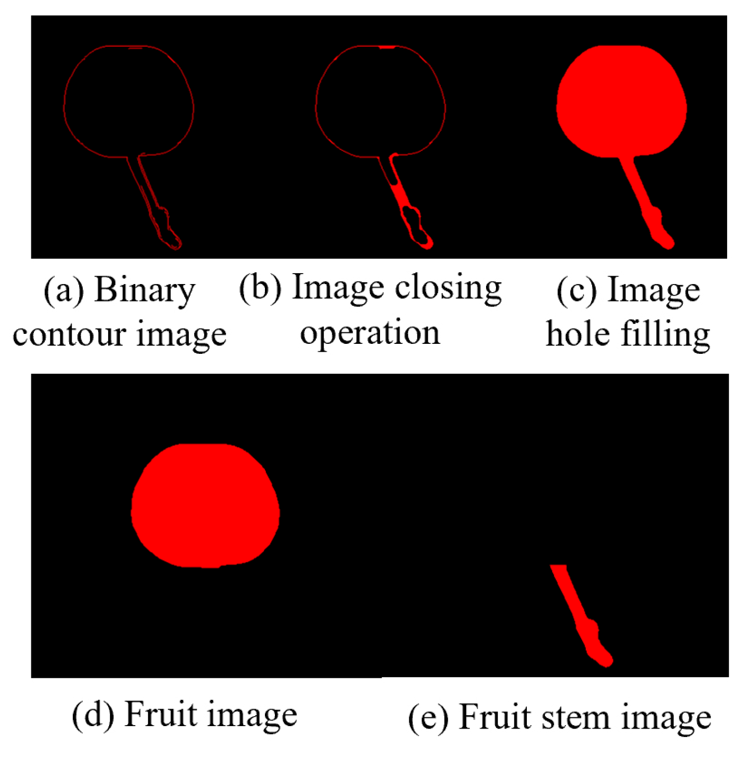
Morphological processing was applied to the binarized image using a closing operation to fully close the binarized contour lines and hole filling to obtain a complete binarized image of the cherry.
Finally, stem separation processing is required for the image. A binarized image of the fruit was obtained by applying the opening operation to the morphological processing. Subtracting the binary image of the complete cherry from the binary image of the cherry fruit through image subtraction produced a binary image of the cherry stem, achieving stem separation.
Figure 5.
Images related to morphological processing.
Cherry size was measured using a binary image of the fruit. According to the newly revised GB/T 26906-2024 “Sweet Cherry” standard, the size specifications of the cherries were classified based on the transverse diameter (d) of the fruit, as outlined in the table below (Table 1). Therefore, it is necessary to measure the transverse diameter of the cherry.
2.5. Pattern Matching and Coordinate System Establishment
Before performing size measurements, it is essential to determine the position and orientation of the cherry fruit in the 2D plane and establish a coordinate system based on its location and orientation to measure the transverse diameter of the cherry. This can be achieved using a geometric matching algorithm that identifies the position and orientation by learning the geometric features of the provided template and the spatial relationships between these features. These combined features form a set that describes the image, and the algorithm performs feature matching with the detected image using this set. In this study, an edge-based geometric matching algorithm was applied to calculate the gradient values of the edges, which were points along the contour found in the image. The algorithm then used these gradient values and point positions to perform matching from the template center. As the cherry image was previously segmented from the background, the current image was free from environmental interference. To increase the robustness, the matching score can be lowered by setting the parameters, allowing for a greater tolerance of different cherry shapes. The matching results are shown in Figure 6.
The figure shows that cherries of varying shapes, positions, and angles were accurately identified, and the corresponding coordinate systems were successfully established.
2.6. Calibration
After establishing the coordinate system, calibration was required. Typically, the imaging model of the camera follows the pinhole imaging method, as shown in Figure 7.
Camera calibration was required to determine the geometric position of a specific point on an object in space and its relationship with other points. This process involved converting the relationships among the world coordinate system, camera coordinate system, image coordinate system, and pixel coordinate system, with the goal of transforming 3D world coordinates into 2D pixel coordinates in the image.
The transformations between these coordinate systems are shown in Figure 8. Similar coordinate transformation methods have been successfully applied in agricultural product measurement studies [19,20].
The relevant formulae are as follows.
Transformation from world coordinates to camera coordinates
Transformation from camera coordinates to image coordinates
Transformation from image coordinates to pixel coordinates
After combining the formulas, we obtain
where is the intrinsic matrix of the camera; is the perspective projection matrix; and is the scaling factor.
Using the above formulas, the conversion between the world and pixel coordinates can be achieved. Once the pixel coordinates were obtained, the distance between two points could be determined by counting the number of pixels between them. According to the previously discussed pinhole imaging principle, a proportional relationship was observed between the distance between the two points in the real world and the corresponding distance in the image (Figure 9).
This relationship can be expressed by the following formula:
where X represents the distance between two points in the real world, x represents the number of pixels between the two points in the image, and Y and y follow the same logic. The formula indicates a proportional factor P between the real-world distance between two points and the number of pixels in the image. This factor, known as pixel equivalent, represents the real-world distance corresponding to a single pixel in an image and can be expressed using the following formula:
The calibration involved manually determining the pixel equivalent, P. The computer then used this pixel equivalent multiplied by the number of pixels between the two points to calculate the real-world distance between them.
In this study, a distortion-free camera was used. Therefore, the captured images were distortion-free. Therefore, traditional camera calibration methods can be employed, focusing only on the spatial coordinate transformation without accounting for distortion. After calibration, the cherry size was measured by defining a ROI and establishing its relationship with the coordinate system, enabling the direct measurement of the cherry’s transverse diameter.
2.7. Measurement System Interface and Related Programs
The system was programmed using LabVIEW, incorporating Machine and Vision modules for machine vision algorithm processing. In addition to basic image acquisition and morphological processing, including the Canny algorithm, the program featured three sub-VIs that encapsulated the flat-field correction module, calibration module, and pattern matching and coordinate system establishment module.
The flowchart of the flat-field correction module shown in Figure 10 illustrates how this module removes environmental interference and enhances the accuracy of the system.
The calibration module facilitates coordinate transformations within the system. The program flowchart is shown in Figure 11.
The pattern-matching and coordinate-system establishment module identified the position and orientation of the fruit and established the corresponding coordinate system. The program flowchart is shown in Figure 12.
The overall system program is illustrated in Figure 13.
The main system interface and related device diagrams are shown in Figure 14.
3. Results
To verify the accuracy of the system measurements, the cherries were used as an example, with both manual and system measurements conducted ten times each. The results of the manual and system measurements are presented below.

Table 2.
Comparison of manual measurement and system measurement results.
| Number of measurements | Manual measurement (mm) | System measurement (mm) | Absolute error (mm) | Relative error (%) |
|---|---|---|---|---|
| 1 | 21.63 | 21.66 | 0.03 | 0.00139 |
| 2 | 21.53 | 21.66 | 0.13 | 0.00604 |
| 3 | 21.47 | 21.66 | 0.19 | 0.00885 |
| 4 | 21.67 | 21.53 | 0.14 | 0.00646 |
| 5 | 21.69 | 21.53 | 0.16 | 0.00738 |
| 6 | 21.71 | 21.53 | 0.18 | 0.00830 |
| 7 | 21.81 | 21.53 | 0.28 | 0.01284 |
| 8 | 21.44 | 21.41 | 0.03 | 0.00139 |
| 9 | 21.55 | 21.66 | 0.11 | 0.00510 |
| 10 | 21.75 | 21.53 | 0.22 | 0.01012 |
| Average of manual measurement | 21.6500 | Standard deviation of manual measurement |
0.1267 | |
| Average of system measurement | 21.5740 | Standard deviation of system measurement |
0.0828 | |
| Average absolute error |
0.0760 | |||
| Average relative error |
0.0035 |
The measurement results revealed that the average value of the system measurements differed from the manual measurements by only 0.0760 mm with an average relative error of 0.35%. Moreover, the standard deviation of the system measurements was 0.0828, which was significantly smaller than that of manual measurements, indicating that the system measurements were more precise and consistent.
To further validate the applicability of the measurement system to small- and medium-sized fruits, measurements were conducted on cherries, blueberries, and walnuts. The results shown in Figure 15, Figure 16 and Figure 17 indicated the RMSE values of 0.32 mm for cherries, 0.29 mm for blueberries, and 0.34 mm for walnuts, with corresponding MAPE values of 0.78%, 2.08%, and 0.90%. This confirmed the high accuracy of the system in obtaining size information for small- and medium-sized fruits. Additionally, the manual measurement of a single fruit took 2.4 s, while the system measurement averaged only 0.4 s per fruit, demonstrating that the system significantly reduced the measurement time and improved the efficiency. This level of automation accuracy aligns with the performance reported in recent machine vision-based automatic recognition systems [15].
4. Discussion
Currently, the size measurement of small fruits is predominantly performed manually, resulting in high labor intensity, lengthy measurement periods, and significant uncertainty in results due to human factors. This issue is especially severe in research institutes where large numbers of samples require size measurements, whether for breeding research or germplasm resource evaluation.
For instance, the Fruit Germplasm Resource Innovation Team at the Shandong Institute of Pomology has preserved over 200 varieties of cherry germplasm and cultivated more than 2,000 seedlings and hybrids. With at least five fruits measured per variety, more than 11,000 samples were required for measurement. This process requires significant human resources and incurs substantial material and time costs. Additionally, small- and medium-sized fruits, such as cherries and blueberries, require high precision and efficiency in measurement owing to their short maturation period and limited shelf life, making traditional manual methods increasingly inadequate for modern agricultural breeding research.
This study developed a size measurement device for small- and medium-sized fruits using LabVIEW. The device processes images to obtain binary representations of the fruit and establishes the relationship between pixels and world coordinates to acquire accurate size information, addressing the challenge of measuring small- and medium-sized fruits. By applying morphological processing, such as opening operations, to remove interfering elements, such as stems, the device minimized the morphological differences between fruits in the images, enhancing its versatility. The system achieved an average relative error of only 0.35% and a standard deviation of 0.0828, demonstrating higher accuracy than manual measurements. The comparison of the system’s measurements with the manual measurements for cherries, blueberries, and walnuts demonstrated small RMSE and MAPE values, with RMSE of 0.32, 0.29, and 0.34 mm, and MAPE of 0.78%, 2.08%, and 0.90%, respectively, confirming the device’s precision and versatility across different fruit types.
This study conducted size measurements exclusively in a laboratory environment, and the device lacked portability, thus limiting it to a single measurement setting. Future research should aim to improve its portability and anti-interference capabilities to adapt to the complex conditions of orchards, allowing for on-site sample collection and measurement.
Author Contributions
Methodology, Y.L. and Z.Z.; Validation, R.X. and J.W.; Formal analysis, R.X. and D.Z.; Writing—review and editing, D.Z. and Q.L.; Writing—original draft, R.X.; Project administration, Q.L. All authors have read and agreed to the published version of the manuscript.
Funding
This work was supported by the Key R&D Program of Shandong Province, China (2023LZGC016; 2022TZXD006) and the Shandong Provincial Natural Science Foundation (ZR2023QC054).
Data Availability Statement
Data will be made available upon reasonable request.
Conflicts of Interest
The authors declare that they have no known competing financial interests or personal relationships that could have appeared to influence the work reported in this paper.
References
- Jana, S.; Parekh, R.; Sarkar, B. A De novo approach for automatic volume and mass estimation of fruits and vegetables. Optik 2020, 200, 163443. [Google Scholar] [CrossRef]
- Wang, Y.; Zhang, X. Study on the measurement of shape parameters of american ginseng based on image processing technology. J. Huaibei Norm. Univ. (Nat. Sci.) 2017, 38, 49–52. [Google Scholar]
- Lee, J.; Nazki, H.; Baek, J.; Hong, Y.; Lee, M. Artificial Intelligence Approach for Tomato Detection and Mass Estimation in Precision Agriculture. Sustainability 2020, 12, 9138. [Google Scholar] [CrossRef]
- Neupane, C.; Pereira, M.; Koirala, A.; Walsh, K.B. Fruit Sizing in Orchard: A Review from Caliper to Machine Vision with Deep Learning. Sensors 2023, 23, 3868. [Google Scholar] [CrossRef] [PubMed]
- Chiranjivi, N.; Maisa, P.; Anand, K.; et al. Fruit Sizing in Orchard: A Review from Caliper to Machine Vision with Deep Learning. Sensors 2023, 23, 3868. [Google Scholar] [CrossRef] [PubMed]
- Tu, K.-L.; Li, L.-J.; Yang, L.-M.; Wang, J.-H.; Sun, Q. Selection for high quality pepper seeds by machine vision and classifiers. J. Agric. 2018, 17, 1999–2006. [Google Scholar] [CrossRef]
- Uzal, L.C.; Grinblat, G.L.; Namias, R.; Larese, M.G.; Bianchi, J.S.; Granitto, E.N. Seed-per-pod estimation for plant breeding using deep learning. Comput. Electron. Agric. 2018, 150, 196–204. [Google Scholar] [CrossRef]
- Tu, K.; Cheng, Y.; Ning, C.; Yang, C.; Dong, X.; Cao, H.; Sun, Q. Non-Destructive Viability Discrimination for Individual Scutellaria baicalensis Seeds Based on High-Throughput Phenotyping and Machine Learning. Agriculture 2022, 12, 1616. [Google Scholar] [CrossRef]
- Tu, K.; Wu, W.; Cheng, Y.; Zhang, H.; Xu, Y.; Dong, X.; Wang, M.; Sun, Q. AIseed: An automated image analysis software for high-throughput phenotyping and quality non-destructive testing of individual plant seeds. Comput. Electron. Agric. 2023, 207, 107740. [Google Scholar] [CrossRef]
- Ghimire, A.; Kim, S.-H.; Cho, A.; Jang, N.; Ahn, S.; Islam, M.S.; Mansoor, S.; Chung, Y.S.; Kim, Y. Automatic Evaluation of Soybean Seed Traits Using RGB Image Data and a Python Algorithm. Plants 2023, 12, 3078. [Google Scholar] [CrossRef] [PubMed]
- Koh, J.C.O.; Spangenberg, G.; Kant, S. Automated Machine Learning for High-Throughput Image-Based Plant Phenotyping. Remote Sens. 2021, 13, 858. [Google Scholar] [CrossRef]
- Clohessy, J.W.; Sanjel, S.; O’Brien, G.K.; Barocco, R.; Kumar, S.; Adkins, S.; Tillman, B.; Wright, D.L.; Small, I.M. Development of a high-throughput plant disease symptom severity assessment tool using machine learning image analysis and integrated geolocation. Comput. Electron. Agric. 2021, 184, 106089. [Google Scholar] [CrossRef]
- Falk, K.G.; Jubery, T.; Mirnezami, S.V.; et al. Computer vision and machine learning enabled soybean root phenotyping pipeline. Plant Methods 2020, 16, 5. [Google Scholar] [CrossRef] [PubMed]
- Zhao, B.; Wang, Y.; Fu, J.; Zhao, R.; Li, Y.; Dong, X.; Lv, C.; Jiang, H. Online measuring and size sorting for Perillae based on machine vision. J. Sens. 2020, 2020, 3125708. [Google Scholar] [CrossRef]
- Lu, W.; Lihong, C. Automatic Recognition and Detection System Based on Machine Vision. J. Control Sci. Eng. 2022, 2022, 123456. [Google Scholar]
- Xiang, L.; Gai, J.; Bao, Y.; Yu, J.; Schnable, P.S.; Tang, L. Field-based robotic leaf angle detection and characterization of maize plants using stereo vision and deep convolutional neural networks. J. Field Robot. 2023, 40, 1034–1053. [Google Scholar] [CrossRef]
- Lay, L.; Lee, H.S.; Tayade, R.; Ghimire, A.; Chung, Y.S.; Yoon, Y.; Kim, Y. Evaluation of Soybean Wildfire Prediction via Hyperspectral Imaging. Plants 2023, 12, 901. [Google Scholar] [CrossRef] [PubMed]
- McGuinness, B.; Duke, M.; Au, C.K.; Lim, S.H. Measuring radiata pine seedling morphological features using a machine vision system. Comput. Electron. Agric. 2021, 189, 106355. [Google Scholar] [CrossRef]
- Igathinathane, C.; Pordesimo, L.O.; Batchelor, W.D. Major orthogonal dimensions measurement of food grains by machine vision using ImageJ. Food Res. Int. 2009, 42, 76–84. [Google Scholar] [CrossRef]
- Xu, M.; Chen, S.; Xu, S.; Mu, B.; Ma, Y.; Wu, J.; Zhao, Y. An accurate handheld device to measure log diameter and volume using machine vision technique. Comput. Electron. Agric. 2024, 224, 109130. [Google Scholar] [CrossRef]
Figure 3.
Pixel counts in different directions for each algorithm.
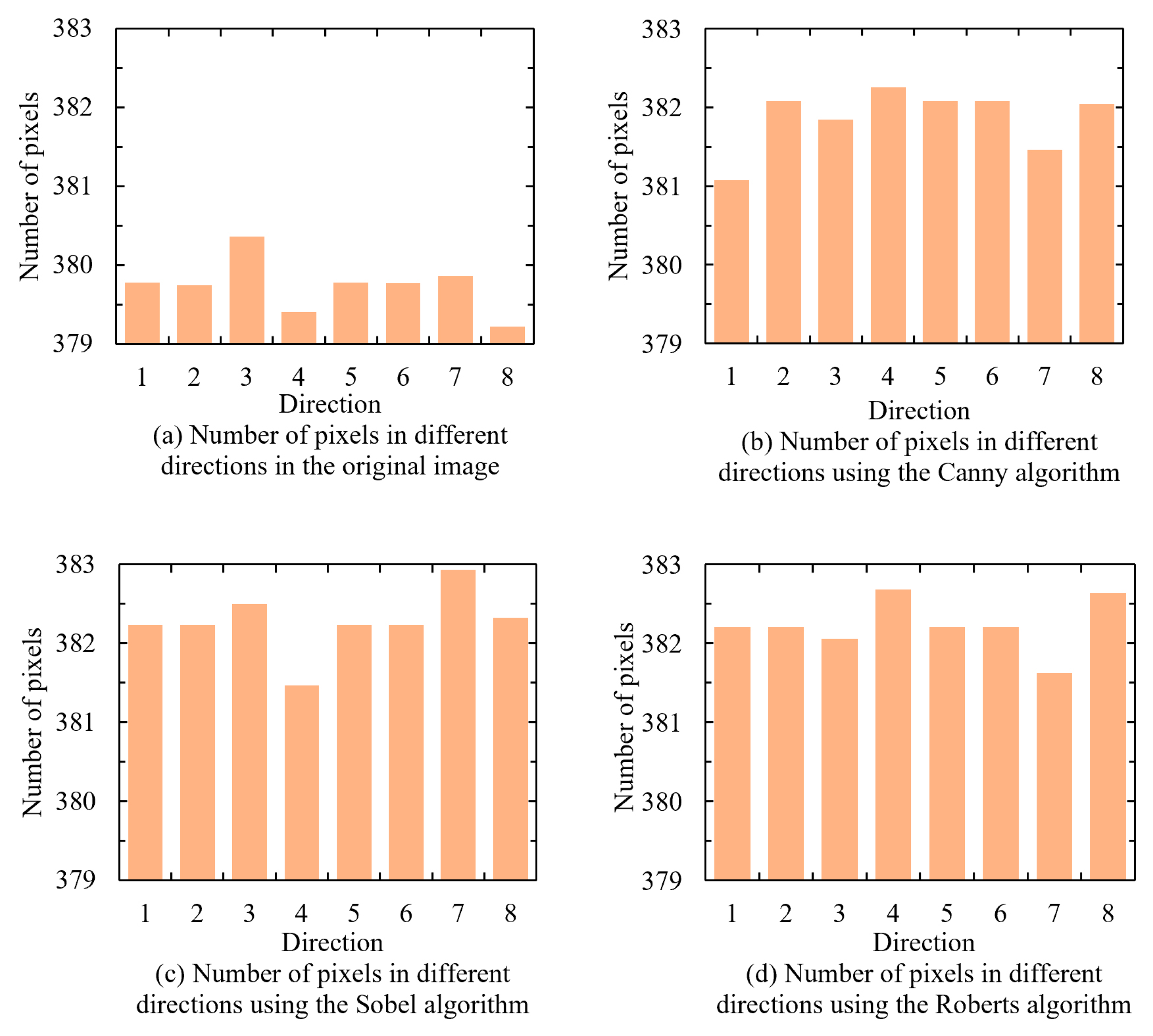
Figure 6.
Matching results for different positions and orientations.
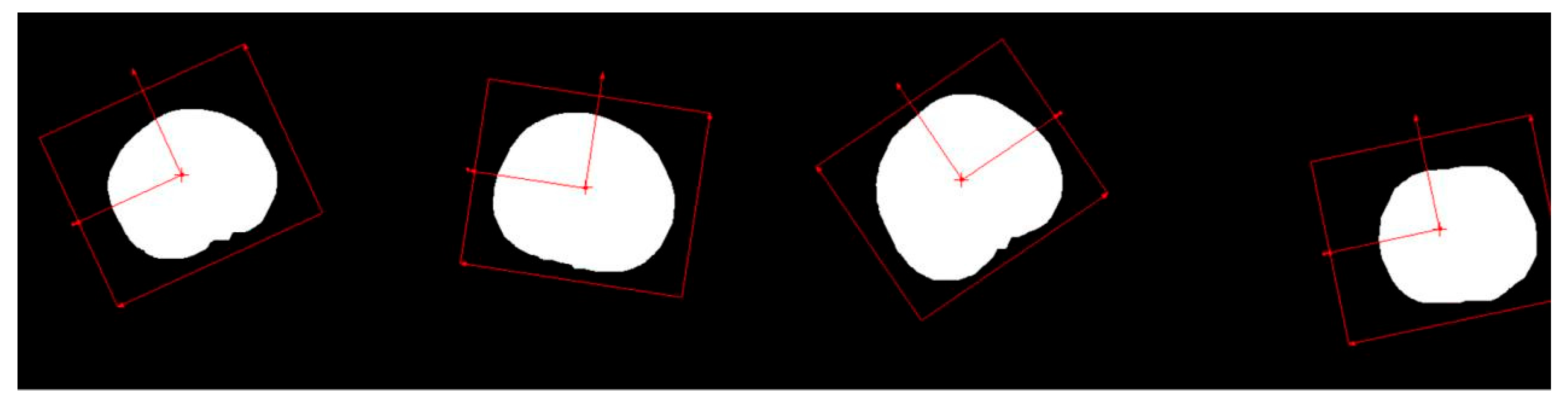
Figure 7.
Imaging principle.
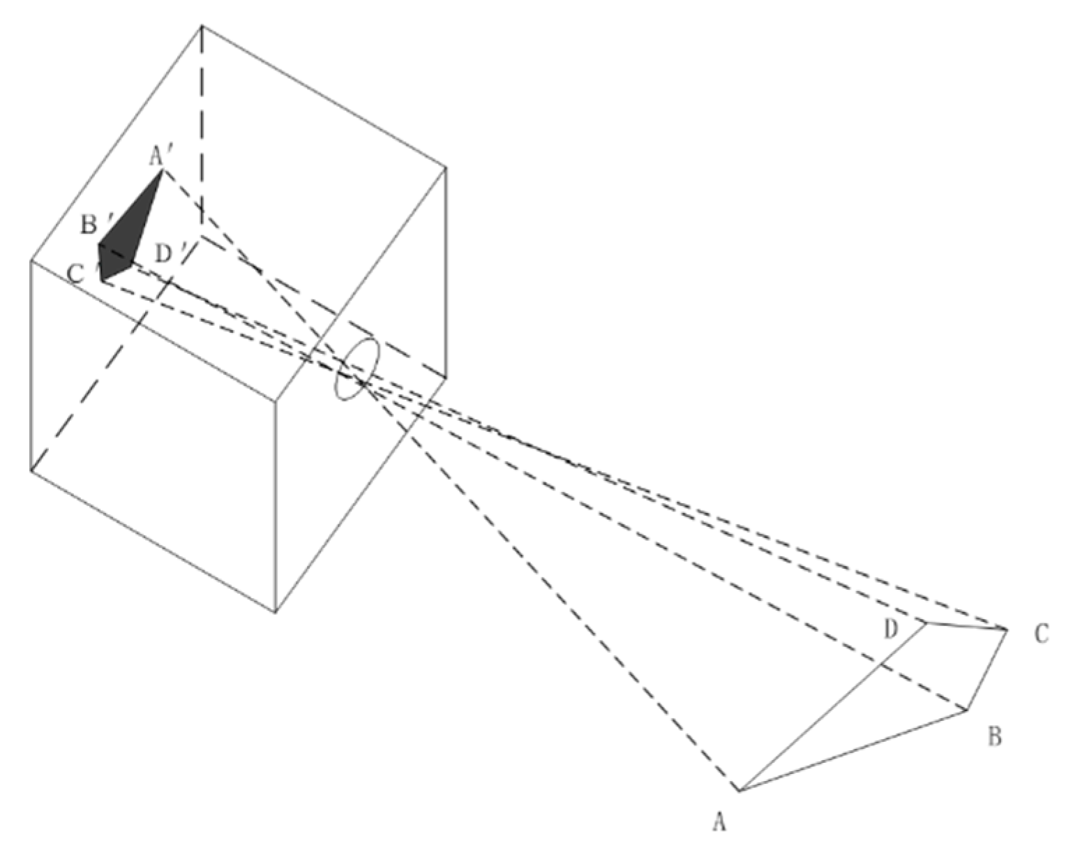
Figure 8.
Coordinate-transformation relationship diagram.
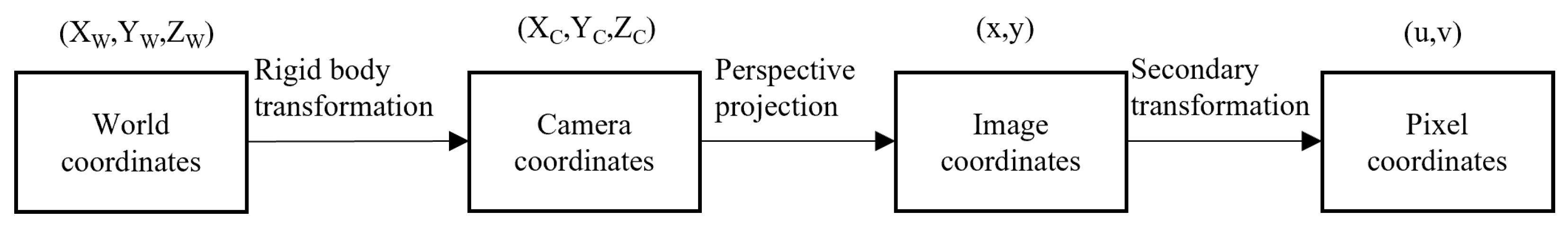
Figure 9.
Size proportional relationship diagram.
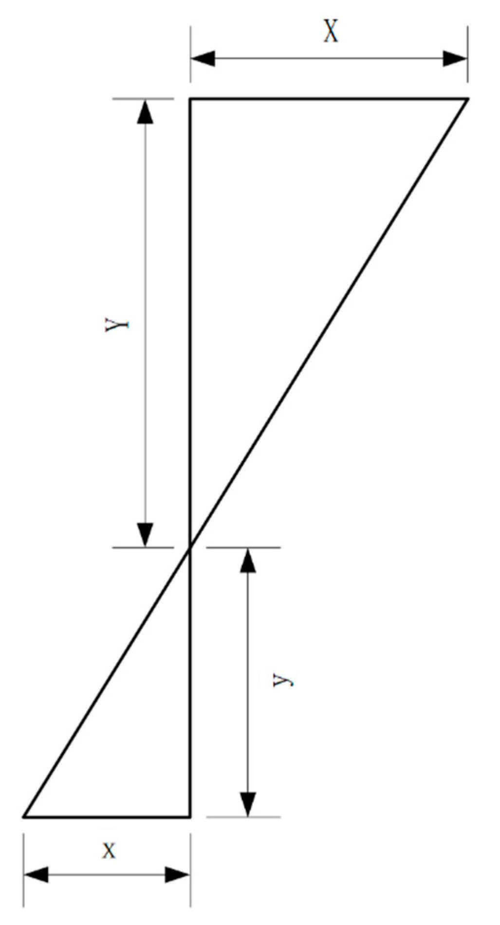
Figure 10.
Program flowchart of flat-field correction.
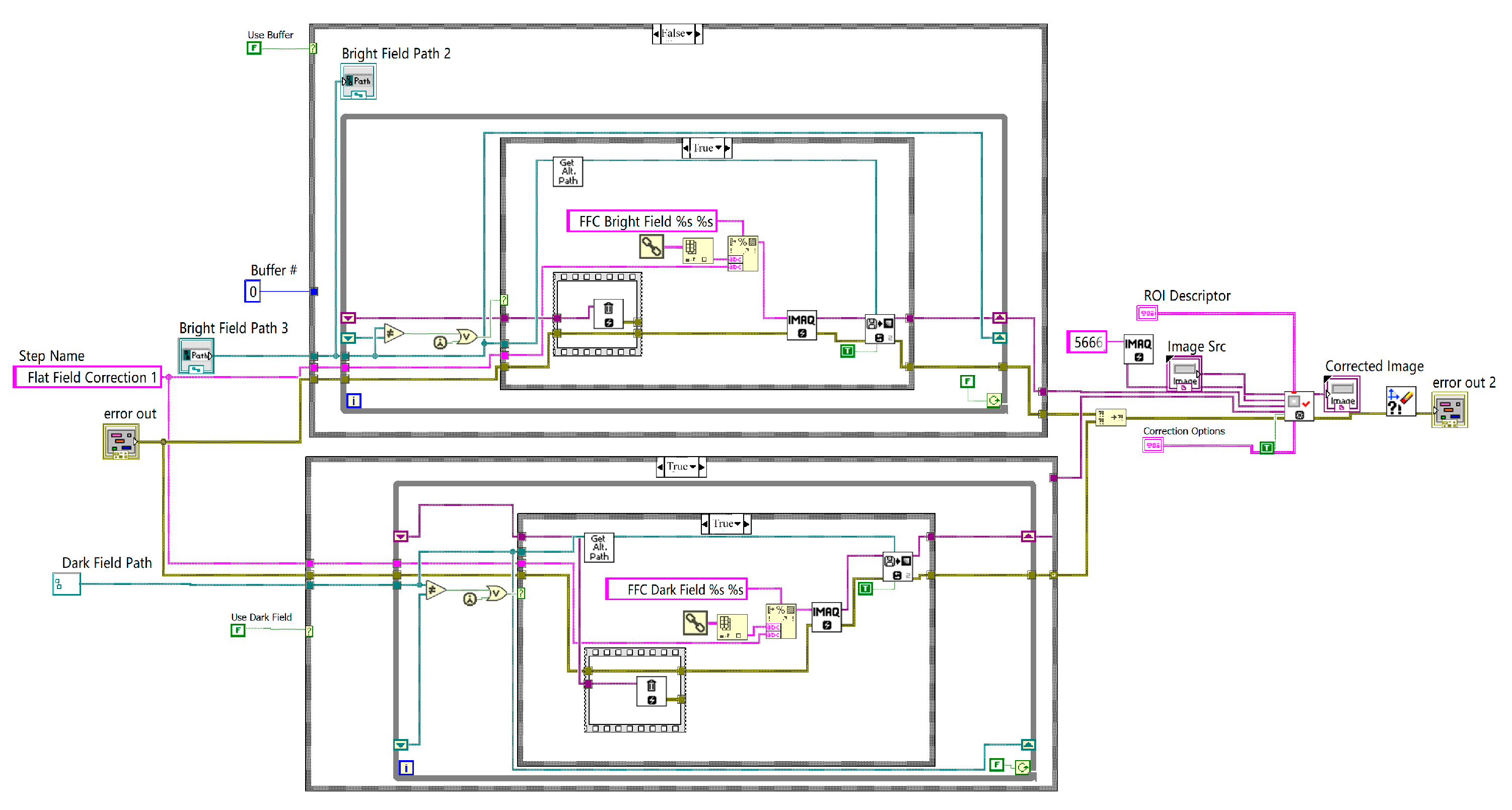
Figure 11.
Calibration program flowchart.
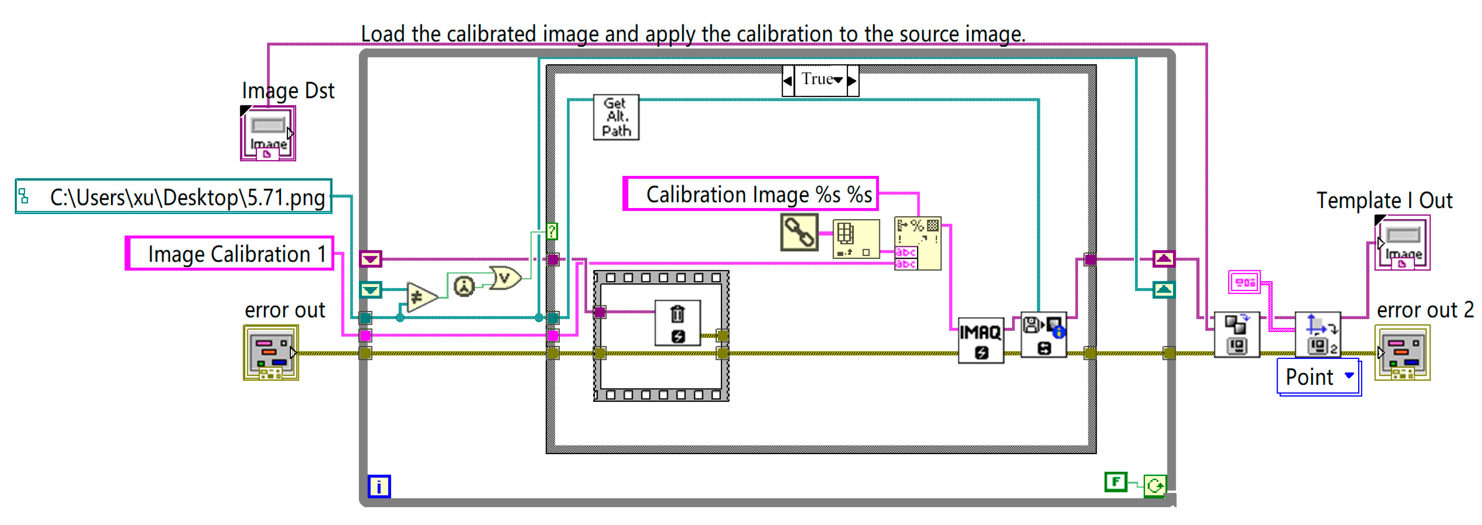
Figure 12.
Program flowchart of pattern matching and coordinate system establishment.
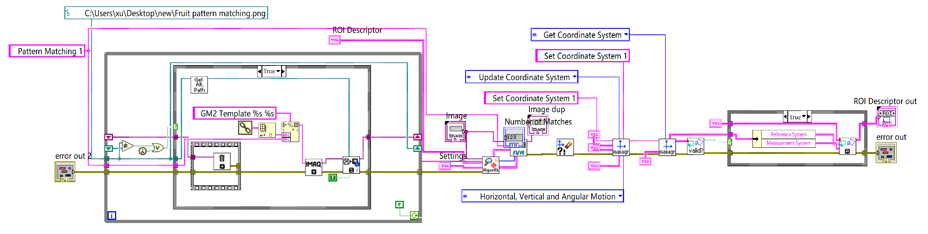
Figure 13.
Overall program flowchart of the cherry-size measurement system.
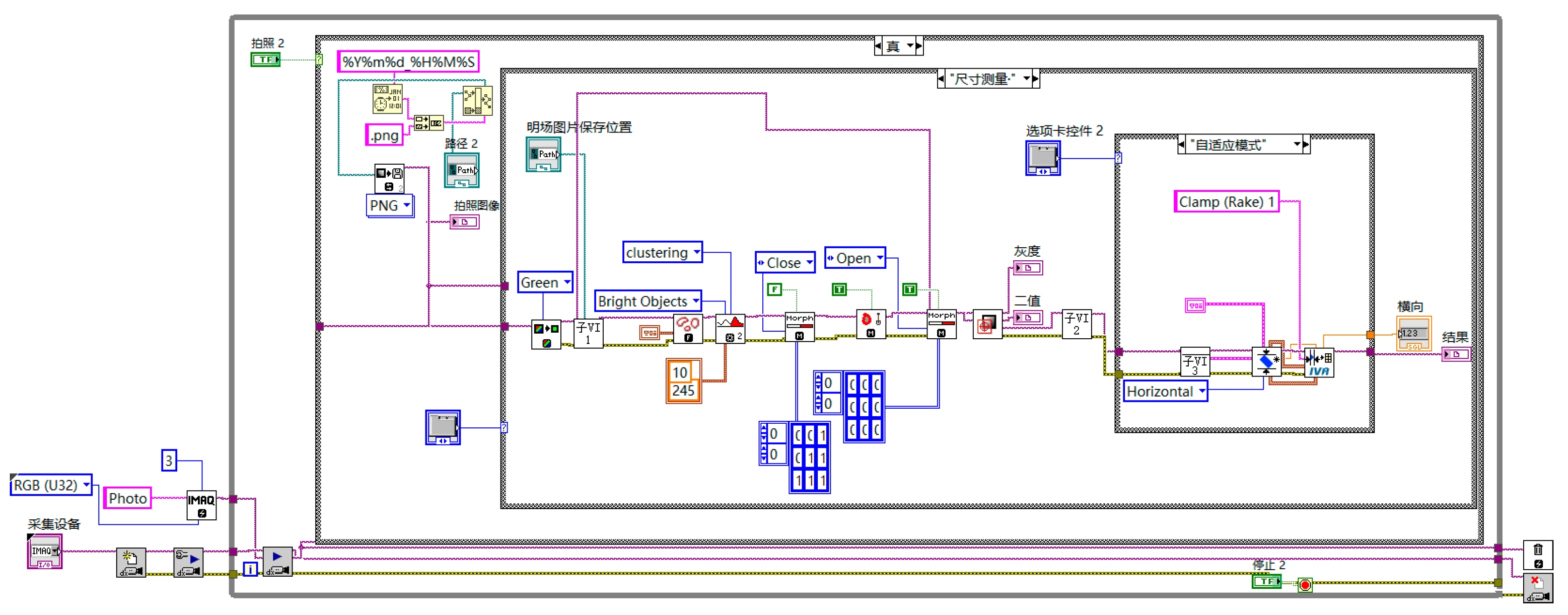
Figure 14.
Size measurement device and system.
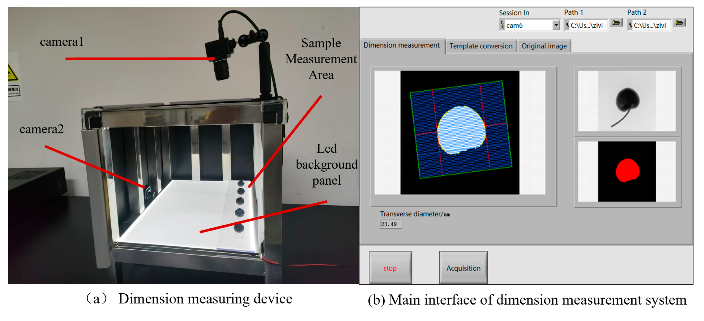
Figure 15.
Accuracy evaluation results for cherries.
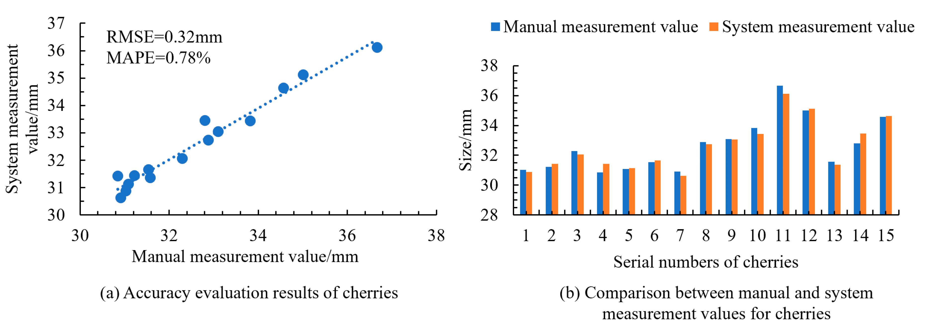
Figure 16.
Accuracy evaluation results for blueberries.
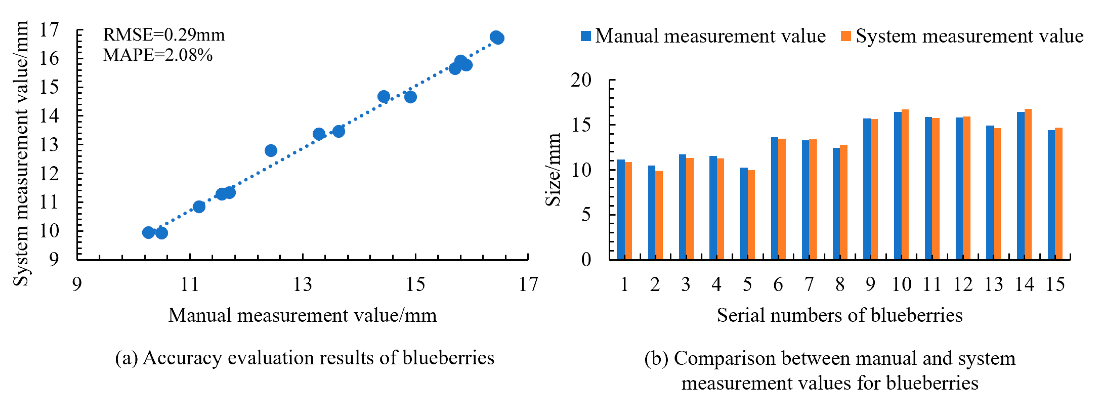
Figure 17.
Accuracy evaluation results for walnuts.
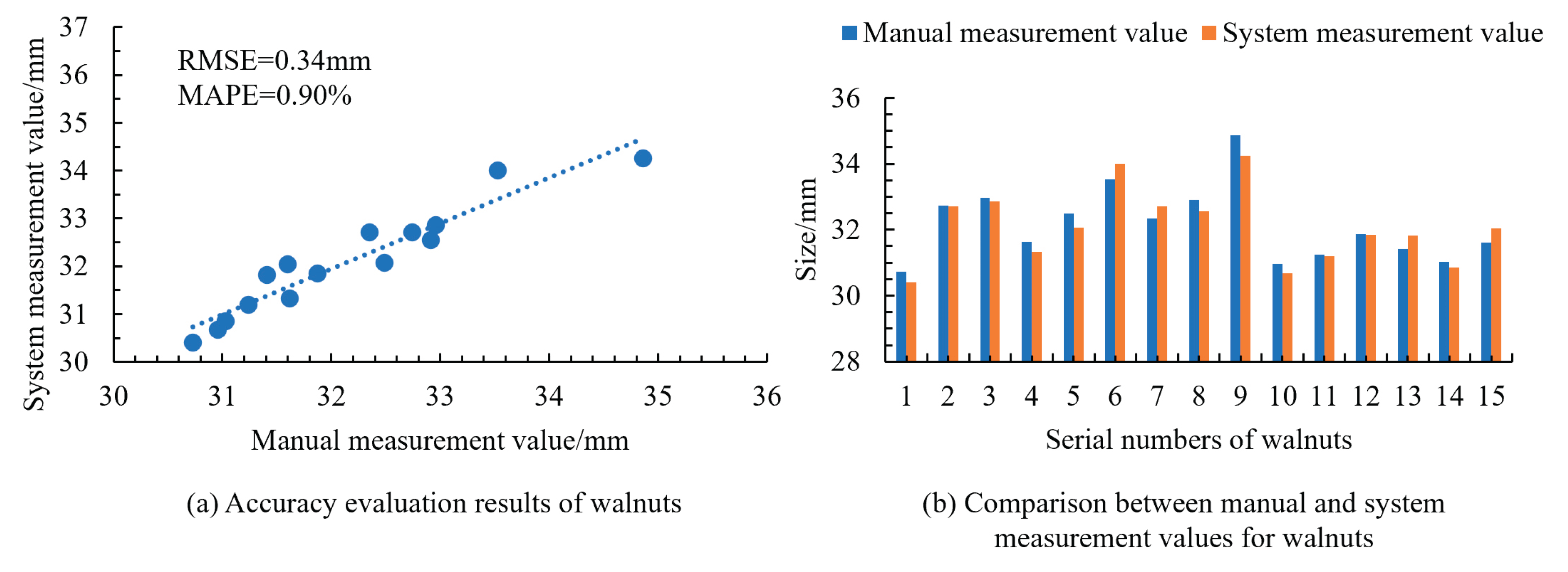
Table 1.
Cherry size specifications.
| Small | Medium | Large | Extra large |
|---|---|---|---|
| d < 24 mm | 24 mm ≤ d < 28 mm | 28 mm ≤ d < 30 mm | d ≥ 30 mm |
Disclaimer/Publisher’s Note: The statements, opinions and data contained in all publications are solely those of the individual author(s) and contributor(s) and not of MDPI and/or the editor(s). MDPI and/or the editor(s) disclaim responsibility for any injury to people or property resulting from any ideas, methods, instructions or products referred to in the content. |
© 2025 by the authors. Licensee MDPI, Basel, Switzerland. This article is an open access article distributed under the terms and conditions of the Creative Commons Attribution (CC BY) license (http://creativecommons.org/licenses/by/4.0/).
Copyright: This open access article is published under a Creative Commons CC BY 4.0 license, which permit the free download, distribution, and reuse, provided that the author and preprint are cited in any reuse.


