Submitted:
15 October 2025
Posted:
16 October 2025
You are already at the latest version
Abstract
This paper explores both Mersenne primes of the form where, is a prime. By extension, the paper also explores Perfect numbers and Sophie primes. Botgh these special primes have a special relationship for “perfectitude”. An insight into these numbers is explored using novel methods that involve the trigonometric functions with integer factorable arguments. Rational functions play a part in the behavior of many functions including regular primes, Mersenne Primes, and Perfect numbers. The paper first determines relationships for primes, and then procedes to show how Perfect number relations can be derived from trigonometric relations. The relationships of trigomentric functions involving the sum of divisors, provide a novel approach to prove that that the analytic structure of cot(x), when split into Mersenne and non-Mersenne classes through the Bernoulli framework, forces a coupling between the two infinite subsets of integers and the contradiction (negative ratio despite all positive terms) is a proof of necessity for infinite balance between both classes. This paper also explores Sophie Germain primes of the form where, is a prime. By extension, the paper also explores other properties of prime numbers. I derive a trigonometric product identity that isolates the condition for a prime p to form a Sophie Germain prime pair, i.e. such that is also prime. The analysis shows that the classical tangent–sine product expansion, when modified by the divisor-sum function, sigma(n), reproduces a constant equality only under this primality constraint.
Keywords:
Mersenne primes
; SOPHIE GERMAIN PRIMES
; Perfect numbers
; abondant numbers
; deficient numbers
; trigonometric functions
; Primes
; Cot
; trigonometry
; sums of divisors
; invariance
1. Introduction
The search for a general formula to determine the Mersenne prime is an ongoing challenge in
mathematics. Mersenne primes are of the form , where is a prime
number, and is also a
prime number. Not all primes can generate a
Mersenne prime. For example,
the primes, 11, 23, 29, are examples that do not generate Mersenne Primes,, they generate what I refer to as Mersenne
Numbers that have the
Mersenne form where is a
non-generating prime, and is not. It is extremely difficult to find the Mersenne
primes, without tedious
factorization, since the known set of Mersenne primes are separated
by long distances of non-primes, Perfect numbers, are numbers defined by the product , where, is a prime that generates a Mersenne prime. They have
the Sum of Divisors relation, These numbers are related to Mersenne primes by the relation, Hence the search for Mersenne primes, is also the search for Perfect numbers, . It is not known in current art if there are
infinitely many Perfect Numbers, and also if there is infinitely many Mersenne
primes, . So far, all are even numbers, and it is still not yet
determined if there are any odd The approach used in this paper on Mersenne Primes, and Perfect numbers, is so far as I know, has not yet been used by
researchers.
The Gamma-function, denoted as , was first introduced by Swiss mathematician
Leonhard Euler [1] 1729. Euler’s deep insights
into -function led to numerous results that provide key
insights into many fields of mathematics including Probability theory and
Statistics. Other major contributions to the development of the -function used in this paper were developed by Carl
Freidman Gauss [2]. Gauss’s work led to the
famous reflection formula of the -function. A key insight into the -function is its multiplicative nature. New results
will be presented in this paper resulting from the properties of the -function. So far, there has been little
development in the additive representation of the -function as a series of simple terms. The form of
the -function [3],
p.895:
for real and positive is well known. Here, the
remainder of the series (1) is less than the last term that is retained.
Similar series exists for . It will be significant if other forms of these
series can be found.
The product-form of the -function due to Gauss, provides further insights
into many relations that will be developed in this paper. The product form is
given by, [4], p. 896:
Certain invariant relations of the product -function will be developed in this paper to show
the connections of the -function to other functions, particularly the
Riemann-Zeta function, denoted by . The -function, is defined by the additive series:
The importance of the -function is its relation to the distribution of
primes and the Riemann hypothesis. There is a one-on-one correspondence between
the non-trivial roots of the function and the primes. The -function also has a product relation for primes given by [4], p.
1037;
Both the -function, and the -function are factorable. These two functions are
related by the -function reflection formula developed by Gauss
given by [4], p.1038:
These relations are well studied, and they provide
a wealth of information in Number theory and many disciplines in Mathematics.
In this article, I show new relations that govern Mersenne primes and twin
primes. All these special integer relations are connected in precious way by
powers of .
2. Mersenne Numbers
Mersenne primes were named after the French
philosopher and number theorist, Marin Mersenne (1588-1648). Marin Mersenne was
also a monk and a theologian, and he had an important influence on many
academics such as Fermat, Pascal, Huygens, Descartes and Galileo. He also
inspired the invention of the pendulum clock.
Only a few Mersenne primes, are known to exists. It is an ardous task to
determine whether a Mersenne number, is either a Mersenne prime, prime or a Mersenne number since the computation of factors of large Mersenne
numbers, is very difficult. When is a prime, not all are Mersenne primes, and it is not known whether
there are infinitely many Mersenne primes, . The Great Internet Mersenne Prime Search (GIMPS)
has discovered a new Mersenne prime number, = 282,589,933 - 1. The first few Mersenne primes
are (Online Encyclopedia of Integer Sequences, (OEIS)
#A000668), corresponding to indices 2, 3, 5, 7, 13, 17, 19, 31, 61, 89, 107, 127, 521,
607, 1279, 2203, 2281, 3217, 4253, 4423, 9689, 9941, 11213, 19937, 21701,
23209, 44497, 86243, 110503, 132049, 216091, 756839, 859433, 1257787, 1398269,
2976221, 3021377, 6972593, 13466917, 20996011, 24036583, 25964951, 30402457,
32582657, 37156667, 42643801, 43112609, 57885161… (OEIS A000043).
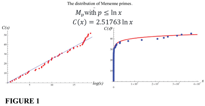
It is conjectured that there exist an infinite
number of Mersenne primes. In Wolfram, we find the best fit line through the
origin to the asymptotic number of Mersenne primes with for the first 51 known Mersenne primes. The
best-fit line gives This fit is illustrated below in Figures 1 and 2. It has been conjectured
without any particularly strong evidence, that the constant is given by , where is the Euler-Mascheroni constant.
In this paper, I will give strong relations for
this constant.
Literature on Mersenne primes is mainly dedicated
to the search for new Mersenne primes, and very few attempts have made progress
on the actual theoretical work. In [8],
Zhaodong Cai, Matthew Faust, A.J. Hildebrand, Junxian Li, and Yuan Zhang
studied theleading digits of the Mersenne primes. They attempted to show that
leading digits of Mersenne numbers behave in many respects more regularly than
some sequences of powers of logs of 2. Further information on Mersenne primes
can be found in [8–11]. In [12] J. Aust yield bounds on the sums of exponents
of Mersenne primes.
Most of this research is related to the present
work only in an attempt to categorize properties that Mersenne primes may have
found to have, however, the present paper does not rely on any of the current
work known on Mersenne primes, but starts a new trend in expoloring the
properties of Mersenne primes. To begin, let us explore the concepts that lead
to the final proof.
3. The Invariance of the Gamma Function to Substitution
I first want to introduce the curious fact that any
function with a relational product can be represented by the Sums of Divisor function. Here is a simple example:
we can put and so,
we can put then, a Perfect number has the relation:
Here is another example:
I we can put and so, applied to the formula [3], p.41:
Interestingly, and , differentiate between odd and even values of Since primes have an even number, and is always even except for the prime 2, the
relations does not apply to primes! Since For example,
By using the sum of divisor function, for Perfect
numbers, the even trigonometric relations apply, but the relations, do not apply, so we can put, . The fact that the sum of divisor function can be manipulated this way leads to some interesting formulas that can produce significant and unexpected results.
4. Application of the Trigonometric Function to Perfect Numbers
A Perfect Number is defined as a number for which A list of some known Perfect numbers is
Hence for, example, in (10), putting then, we have
LEMMA 1: The rational trigonometric
functions determine
Proof:
If is a Perfect number, then, the equality applies
only when.
Taking the limits:
Now,for large values of and so we can approximate the product for large
values of as follows:
Put
For the infinite product we have,
It is clear that there if there exists a continued
set of infinitely large Perfect Numbers then,
Each of these three relations is only true when is a Perfect
number.
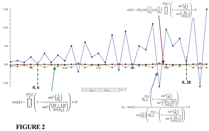
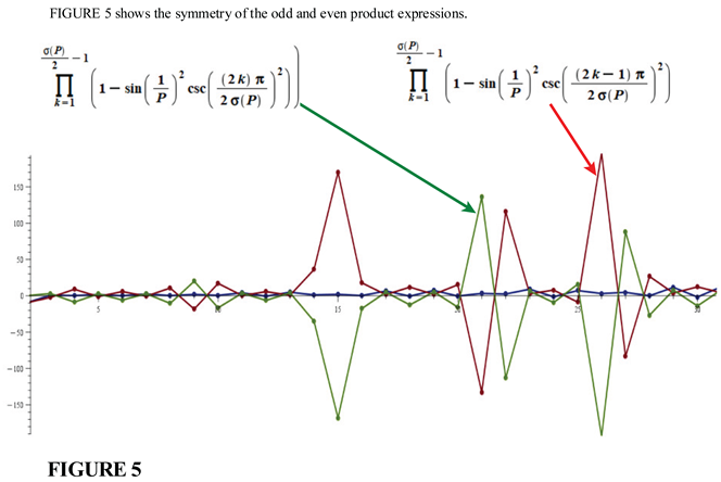
Figure 2
shows the correletion of the relation (27) with Perfect Numbers.
From symmetry, and considering the form for the
divisor function:
Since , where is a prime, we can factor the perfect number as follows:
, where This factorization leads to the following results:
It is clear that the there is a direct
correspondence between the Perfect Number and The graphs of
the two functions is shown in Figure 3.
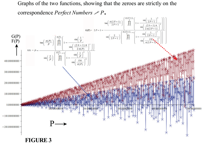
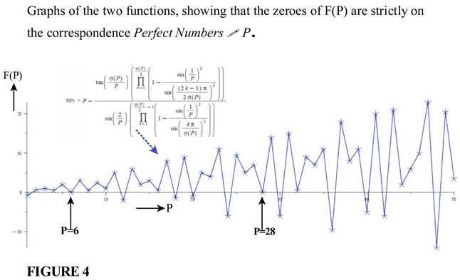
Figure 4
shows the correspondence
The relations (19) hold for all Perfect Numbers. The right hand side of (19) does not depend on implicit rational relationships between and It is clear that the basic rational trigonometric functions capture the properties of integers. We now explore the general forms of trinometric and exponential forms that capture Perfect numbers, Abondant numbers and deficient numbers in one relation.
5. The General Relation That Captures the Behavior of Abondant Numbers, Perfect Numbers and Deficient Numbers
Definition 1:
An Abundant number is a positive integer for which the sum of its proper divisors excluding itself is greater than the number itself.
Definition 2:
A Perfect number is a number for which the sums of all divisors is equal to twice the number.
Definition 3:
A Deficient number is a number for which the sums of all divisors is less than twice the number.
Lemma 2:
If is a Perfect number, then,
Proof: for a Perfect number, Hence,
The distribution of perfect numbers, abondant
numbers and deficient numbers is captured by the general relation:
- For perfect numbers, and the relation (33) vanishes.
- For abondant numbers, and the relation does not vanish but generates negetaive imaginary values for
- For deficient numbers, and the relation does not vanish but generates positive imaginary values for
To see this, put the relation (33) in the form:
Obviously, the zeros of the function (34) occur at
the Perfect numbers. However, for clarity we convert this relation to the
exponential form:
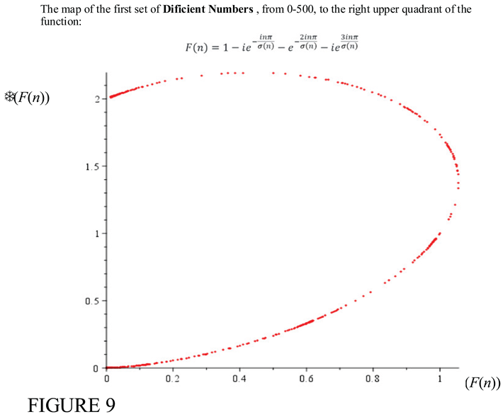
Figure 6
shows the complex map of the function over the range
.
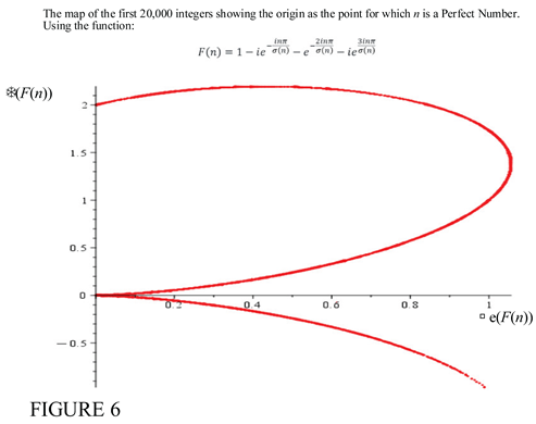
The zeros of the function occur at the values 6, 28, 496, 8124….
NOTE*: The Mersenne primes and the perfect
numbers can only exist on the upper right quadrant corrsponding to deficient
numbers. Perfect numbers are the zeros of the function .
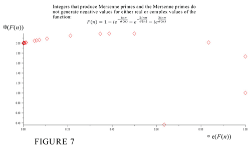
The general locations of primes and Mersenne primes are shown in Figure 7. As can be seen, the oprimes do not generate negative imaginary values, and are located on the top-right quadrant of the complex plane.
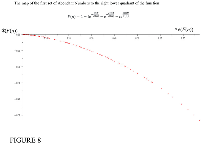
Hence, It is clear that the sequence of abundant numbers, [12, 18, 20, 24, 30, 36, 40, 42, 48, 54, 56, 60, 66, 70, 72, 78, 80, 84, 88, 90, 96, 100, 102, 104, 108, 112, 114, 120, 126, 132, 138, 140, 144, 150, 156, 160, 162, 168, 174, 176, 180, 186, 192, 196, 198, 200, 204, 208, 210, 216, 220, 222, 224, 228, 234, 240, 246, 252, 258, 260, 264, 270, 272, 276, 280, 282, 288, 294, 300, 304, 306, 308, 312, 318, 320, 324, 330, 336, 340, 342, 348, 350, 352, 354, 360, 364, 366, 368, 372, 378, 380, 384, 390, 392, 396, 400, 402, 408, 414, 416, 420, 426, 432, 438, 440, 444, 448, 450, 456, 460, 462, 464, 468, 474, 476, 480, 486, 490, 492, 498, 500], produce values of in (35) that lie on the lower right quadrant of the complex plane. This distinct observation for the first 500, abondant numbers provides a clue as to their distribution.
It is clear the first numbers between 0 and 500 that generate a sequence of deficient numbers:
[2, 3, 4, 5, 7, 8, 9, 10, 11, 13, 14, 15, 16, 17, 19, 21, 22, 23, 25, 26, 27, 29, 31, 32, 33, 34, 35, 37, 38, 39, 41, 43, 44, 45, 46, 47, 49, 50, 51, 52, 53, 55, 57, 58, 59, 61, 62, 63, 64, 65, 67, 68, 69, 71, 73, 74, 75, 76, 77, 79, 81, 82, 83, 85, 86, 87, 89, 91, 92, 93, 94, 95, 97, 98, 99, 101, 103, 105, 106, 107, 109, 110, 111, 113, 115, 116, 117, 118, 119, 121, 122, 123, 124, 125, 127, 128, 129, 130, 131, 133, 134, 135, 136, 137, 139, 141, 142, 143, 145, 146, 147, 148, 149, 151, 152, 153, 154, 155, 157, 158, 159, 161, 163, 164, 165, 166, 167, 169, 170, 171, 172, 173, 175, 177, 178, 179, 181, 182, 183, 184, 185, 187, 188, 189, 190, 191, 193, 194, 195, 197, 199, 201, 202, 203, 205, 206, 207, 209, 211, 212, 213, 214, 215, 217, 218, 219, 221, 223, 225, 226, 227, 229, 230, 231, 232, 233, 235, 236, 237, 238, 239, 241, 242, 243, 244, 245, 247, 248, 249, 250, 251, 253, 254, 255, 256, 257, 259, 261, 262, 263, 265, 266, 267, 268, 269, 271, 273, 274, 275, 277, 278, 279, 281, 283, 284, 285, 286, 287, 289, 290, 291, 292, 293, 295, 296, 297, 298, 299, 301, 302, 303, 305, 307, 309, 310, 311, 313, 314, 315, 316, 317, 319, 321, 322, 323, 325, 326, 327, 328, 329, 331, 332, 333, 334, 335, 337, 338, 339, 341, 343, 344, 345, 346, 347, 349, 351, 353, 355, 356, 357, 358, 359, 361, 362, 363, 365, 367, 369, 370, 371, 373, 374, 375, 376, 377, 379, 381, 382, 383, 385, 386, 387, 388, 389, 391, 393, 394, 395, 397, 398, 399, 401, 403, 404, 405, 406, 407, 409, 410, 411, 412, 413, 415, 417, 418, 419, 421, 422, 423, 424, 425, 427, 428, 429, 430, 431, 433, 434, 435, 436, 437, 439, 441, 442, 443, 445, 446, 447, 449, 451, 452, 453, 454, 455, 457, 458, 459, 461, 463, 465, 466, 467, 469, 470, 471, 472, 473, 475, 477, 478, 479, 481, 482, 483, 484, 485, 487, 488, 489, 491, 493, 494, 495, 497, 499 ], produce values of that lie on the upper right quadrant of the complex plane. This distinct observation for the first 500, defficient numbers and abondant numbers provides a clue as to their distributions.
Between the abondant numbers and the deficient numbers, are the Perfect Numbers, [6, 7, 28, 496, 8128, 33550336,….], that generate the zeros of the function:
Hence, the imaginary part of the function determines if a number is an abondant number, a perfect number or a deficient number.
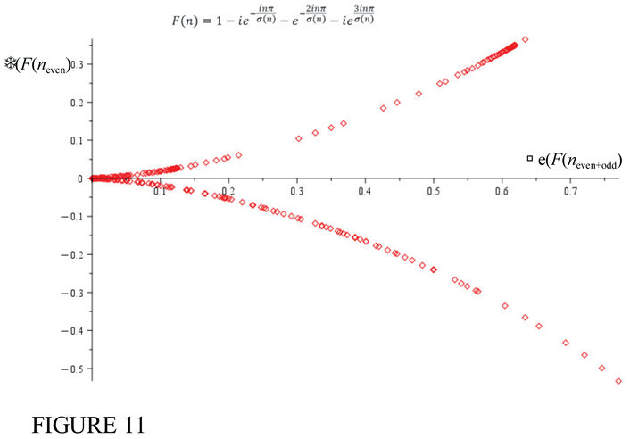
The first set of even numbers from 0..500 that lie on the defient number curve but are not abondant numbers are:
[2, 4, 6, 8, 10, 14, 16, 22, 26, 28, 32, 34, 38, 44, 46, 50, 52, 58, 62, 64, 68, 72, 74, 76, 82, 86, 92, 94, 98, 106, 110, 116, 118, 122, 124, 128, 130, 134, 136, 142, 146, 148, 152, 154, 158, 164, 166, 170, 172, 178, 182, 184, 188, 190, 194, 202, 206, 212, 214, 218, 226, 230, 232, 236, 238, 242, 244, 248, 250, 254, 256, 262, 266, 268, 274, 278, 284, 286, 290, 292, 296, 298, 302, 304, 310, 314, 316, 322, 326, 328, 332, 334, 338, 344, 346, 356, 358, 362, 370, 374, 376, 382, 386, 388, 394, 398, 404, 406, 410, 412, 418, 422, 424, 428, 430, 434, 436, 442, 446, 452, 454, 458, 466, 470, 472, 478, 482, 484, 488, 494, 496].
These numbers are clearly defined by (37).
Figure 10 shows the 2D plot of the function covering both odd and even numbers in the range 0.
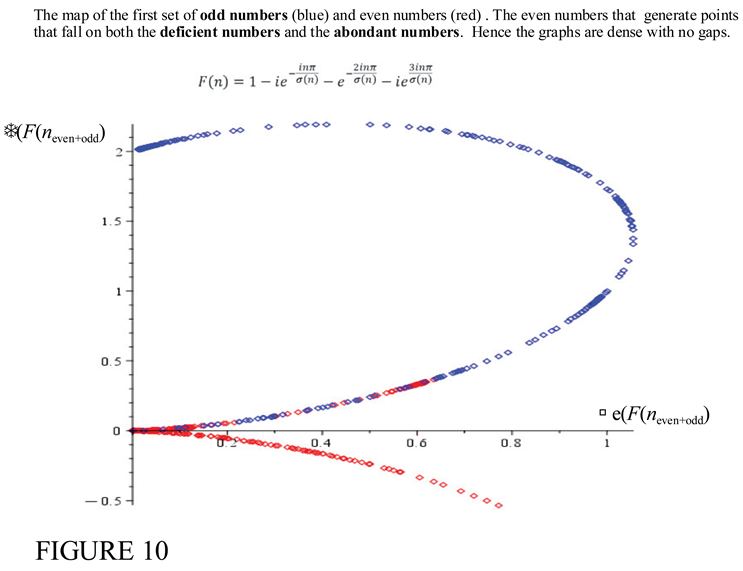
It is clear that the even numbers (red points) can fall on both the deficient number curve and the abondant number curve. The deficient numbers seem to be bounded by the line and a maximum imaginary value of .
Definition 4: An Deficient disturbing number, (DDN), is a deficient number which:
These are the red points on Figure 10 that intermingle with the blue odd number points.
[2,4,8,10,14,16,22,26,32,34,38,44,46,50,52,58,62,64,68,74,76,82,86,92,94,98,106,110,116,118,122,124,128,130,134,136,142,146,148,152,154,158,164,166,170,172,178,182,184,188,190,194,202,206,212,214,218,226,230,232,236,238,242,244,248,250,254,256,262,266,268,274,278,284,286,290,292,296,298,302,310,314,316,322,326,328,332,334,338,344,346,356,358,362,370,374,376,382,386,388,394,398,404,406,410,412,418,422,424,428,430,434,436,442,446,452,454,458,466,470,472,478,482,484,488,494…..].
The extent to which the even numbers infiltrate the deficient number space for up to seems to be confined to the approximate range,
The extent to which the even numbers penetrate the abondant number space is unknown. However it is known that there exists in infinite number of abundant numbers. It has been shown that every multiple is either an abondant number, or taking more multiples of 6 of such numbers leads to an bondant number. Since there is an infinite number of multiples of 6, then there are an infinite number of abondant numbers. Erdos &Graham, 1980, [], showed that even numbers greater than 46 are either abundant numbers or the sum of two abondant numbers.
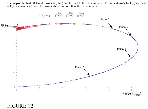
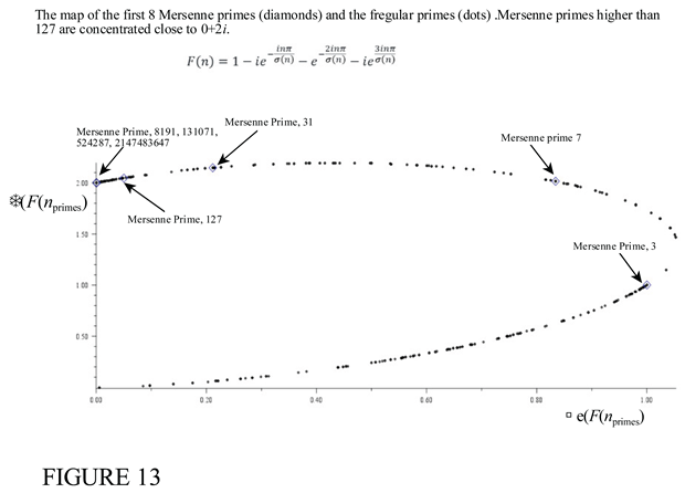
Figure 13 shows the distribution of the Mersenne primes with the regular primes.
6. The Extension of TH Function F(n) to a General Series Form
The function
behaves like a CyclotomicPolynomial. CyclotomicPolynomialare the minimal polynomials of primitive roots of unity with rational coefficients. The first few CyclotomicPolynomial are shown below:
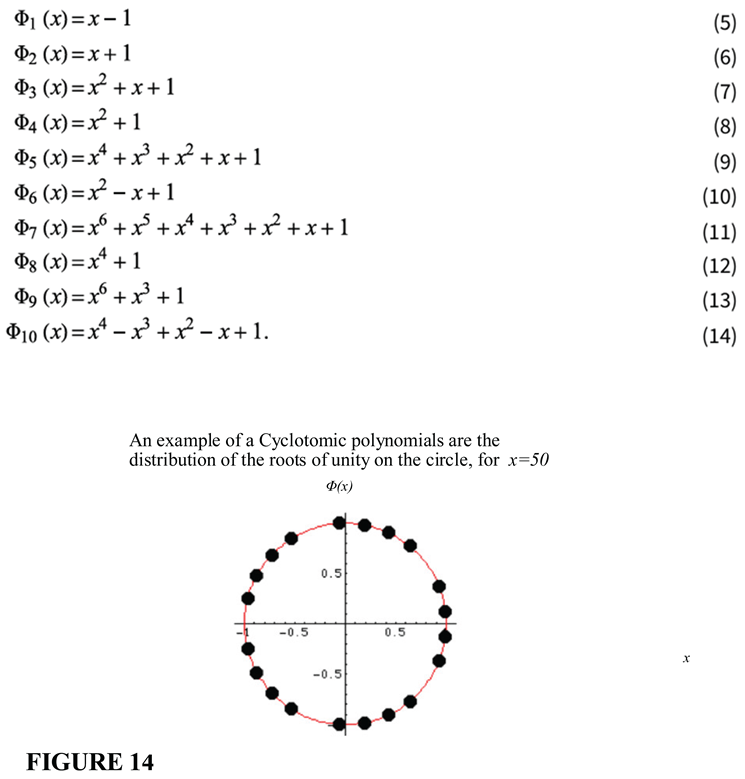
A cyclotomic polynomial is of the product form:
where, , are the roots of unity in the complex plane, . In general, the circle, and is taken over integers relative prime to It is clear that the function
is composed of functions of cyclotomic polynomials for the the special case of an expansion of some function over the function Looking at exponential terms with the sequence, we determine the first difference in the powers to be
The second difference gives,
The second difference points to the function following a sequence of powers that is purely linear, but quadratic or alternating in some manner. We assume a quadratic relation, of the form, However, the second differences are not the same constants, and so a recurrence relation of the form, must be used to expand as a series of higher powers for recurrenses. The sequence of powers in follows the recurrence, with initial conditions,
The characteristic equation for the recurrence then yeilds,
This yields, the two solutions,
Since the recurrence (46) follows a second order linear form, the general solution of the recurrence is
Solcing for and we get:
Hence we get
Hence we have the general form for terms:
This sum produces the first four terms giving the same function:
The function,
will only have coefficients that are 1, or , for the first 4 terms, . The remaining terms have large coefficients that blow up quickly. For example for m=7,
In general, for Perfect numbers,
In general, we have:
| k | |
| 6 | |
| 7 | |
| 8 | |
| 9 | |
| 10 |
A 3-d plot of the function, shows that the function is the axis of an infinite cylinder, where the rest of the terms lie.
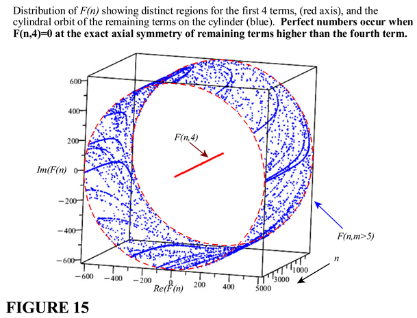
Figure 15 shows the cylinderical form with the axis approaching a line when the cylinder radius approaches infinity. The axis of the cylinder becomes the solutions for Perfect numbers,
Now, from (19), for some integer ,
7. Analytic Mersenne Density and Infinitude
Setup:
Let
Fix Partition, into disjoint classes , and where is the set of Mersenne exponents with a prime.
Define
Note and for
Definition (analytic Mersenne density).
With the set up above, at a fixed suppose the following holds true:
(H1) (Regularity/positivity of coefficients).
Each summand is positive and satisfies the classical Bernoulli-Zeta representation:
Hence,
(H2): (Analytic density at). The decomposition of ields a normalized quadratic identity in the as shown in LEMMA 2, only if LEMMA1 holds.
(H2): (Single valuedness/discriminat collapse). Since is single valued, the discriminat of the quadratic in LEMMA 2 vanishes.
Proof Sketch:
Absolute positivity and conditional subtraction.
By (H1), , and . The analytic value may be negative (e.g., ), which arises from subtracting the strictly positive from .
Quadratic normalization.
(H2) encodes the partition into a quadratic in :
Since and , we have and finite and nonzero.
Discriminant collapse and consistency.
By (H3), . Solve for : the two roots coincide, so the quadratic exactly reproduces .
Contradiction from finiteness.
Assume , is finite. Then is a fixed positive constant, hence is fixed. Meanwhile is also fixed. The identity becomes a rational equality among strictly positive finite constants. But this equality must be compatible with the sign of (e.g., negative at ); when the decomposition is realized by finite sets, the resulting rational combination cannot produce the required analytic sign/phase (it stays on the “algebraic” positive side). This contradicts the actual value of .
A symmetric argument applies if is finite: then is fixed and must bear the entire analytic burden; again the finite rational identity cannot reproduce the analytic sign at . Therefore, both classes must be infinite.
Interpretation via classical pillars.
Pringsheim (nonnegative coefficients ⇒ real singular control): Positivity of coefficients yields rigid real-axis behavior of generating series; finite truncations cannot emulate the required analytic sign at .
Gap/lacunary theorems (Fabry/Hadamard): Attempting to realize the analytic function from a set with “large gaps” (finite or too-sparse) obstructs continuation/phase needed at ; an infinite contribution from both parts is necessary.
Tauberian philosophy (Wiener–Ikehara): Analytic constraints (here, the discriminant identity at a real point) force “density/infinity-type” conclusions for the underlying index sets. Thus both and must be infinite.
Corollary A (Intrinsic analytic density)
Under the hypotheses of the intrinsic analytic Mersenne density
is well-defined with . In particular, cannot be realized by a finite index set on either side.
Theorem 1:
There exists an infinite number of Mersenne Primes.
Proof:
I start with the relationship between Perfect numbers and their sums of divisors. Let be a prime number such that Then the following applies.
Lemma 3:
If
Proof of LEMMA 3: See equation (19) for Perfect numbers.
Lemma 4:
Let p be a prime that generates a Mersenne prime and a Perfect Number N, then, there exits a unique decomposition of
into a quadratic identity
Proof (LEMMA 4):
Now, from [4], p.42, 1.411 (7) we find an expressions for :
Factoring this form into
We find that by chosing , since (66) holds for the expression can be modifed and separated into two class, one over the sum over Mersenne primes to include Perfect numbers, when , a prime for which is a Mersenne prime, and the class of non-Mersenne primes, for
Put in (67), then,
From (19), LEMMA 1, for some Perfect number chosen among the set of
Hence we can multiply by 1,
Divide by .
Now, we reduce (73) further with the following identities [[4],page 41]:
Putting , where Q is a constant associated with .
Substitute expressions (74) into (73):
Note that the sum for the Special primes expressed in Mersernne Primes require a modification with the factor for the original sum defoinition for .
Let
Then,
However, by (H3), can only have one value, and since is positive, hence, we get:
However, if is a Special prime, (a Perfect number, then, and thus, using the negative value of the square root,
A similar analysis for Sophie primes gives the following.
8. Application of the Trigonometric Function to Sophie Germain Numbers
A Sophie Germain primes is defined as a number for which Consequently, since both numbers are primes, we have
This is very intimately related to Perfect numbers were,
Hence for, example, in (8), putting then, we have
Lemma 5: The rational trigonometric functions determine Proof: From (15),
This is the relation for Perfect Number, and so we arrive at: If is a Perfect number, then, the equality applies only when. Since , we have,
Hence the rational functions of the function in the trigonometric functions encodes this behavior of various types of numbers classes.
For Sophie Germain primes, we have:
Then, since
Equation (94) only holds for Sophie Germain Primes. Hence we find that (18) behave distinctly for the sets of Mersenne primes that yield Perfect numbers , while (94) behaves distinctly for Sophie Germain primes . The connection between the two suggest that the infinitum condition applies equally to both sets of numbers iff it applies to one or the other. Perfect numbers are dealt with in a yet unpublished paper “There are infinitely many Mersenne Primes”, MDPI: Manuscript ID:mathematics-3942588.
The relations (94) hold exclusively for all Sophie Germain Primes. The right hand side of (20) depends on implicit rational relationships between and It is clear that the basic rational trigonometric functions capture the properties of special prime integers. We now explore the general forms of trinometric and exponential forms that capture Sophie Germain Primes.
Multiply by
Putting , in (51), then,
Then,
However, by (H3), can only have one value,and since is positive, hence, we get:
However, if is a Special prime, then, and thus, using the negative value of the square root,
is transcendental, so any finite algebraic or rational sum (like a finite Bernoulli sum) can never equal . This conclusion is supported by the following theorems.
The symmetry of both Perfect numbers and Sophie primes is a general result of the cot-function for these special primes. Now is transcendental, so any finite algebraic or rational sum (like a finite Bernoulli sum) can never equal . This conclusion is supported by the following theorems.
- Fabry/Hadamard (sparsity ↔ analytic behavior) [5]: The Fabry and Hadamard theorems, particularly the gap theorems, are central results in complex analysis concerning the analytic continuation of power series with “lacunary” or gapped coefficients. Both theorems establish conditions under which a power series cannot be analytically extended beyond its circle of convergence, which then becomes a “natural boundary” for the function.
- Lindemann–Weierstrass Theorem (1885) [6]:
Ifare distinct algebraic numbers, then the numbersare linearly independent over the algebraic numbers.
These are classical results implying that for any nonzero algebraic a,
are all transcendental. This guarantees that (with 2 algebraic) is transcendental, so any finite algebraic or rational sum (like a finite Bernoulli sum) can never equal . Hence, equality must involve an infinite series and provides a perfect analytical foundation for the infinitude of Special primes.
- c.
- Siegel–Shidlovsky Theorem (1956) [7]
Ifsatisfy a linear differential system with algebraic coefficients andis algebraic, then the set of valuesthat are algebraic is “exceptionally small.
For most analytic functions, values at algebraic points are transcendental. Bernoulli numbers arise from expansions of , which satisfies such a differential equation. Then, is an evaluation of a linear combination of such special-function values at By Siegel–Shidlovsky, its transcendence cannot arise from a finite truncation and only the infinite series can reproduce a transcendental constant. Thus, finite truncations are algebraic, but the limit equals (transcendental), forcing infinitely many contributing terms.
- d.
- Baker’s Theorem (1966) on Linear Forms in Logarithms [8].
Any nontrivial linear combination of logarithms of algebraic numbers with algebraic coefficients is transcendental.
The Bernoulli numbers and trigonometric expansions can both be expressed via logarithmic integrals (e.g., Euler–Maclaurin, zeta relations). This means any equality of the form would imply a linear relation between logarithms of algebraic numbers. This is impossible by Baker’s theorem [8]. Therefore, the equality holds only as an infinite sum.
- e.
- Nesterenko’s Theorem (1996) [9] on the algebraic independence of
Certain combinations of transcendental constants (including trigonometric values at algebraic arguments) are algebraically independent over.
This determines that cot(2) cannot be algebraically dependent on any rational or Bernoulli-type term. Thus, no finite algebraic structure The Bernoulli-weighted Special-prime sum structurally resembles these zeta-type series. By analogy, the equality with cot(2) is consistent with the class of transcendental series equalities known to require infinite index sets.
Lemma 6: (Transcendental Consistency Condition).
By the Lindemann–Weierstrass theorem [6], cot(2) is transcendental. Since every partial Bernoulli sum in primes such as
is algebraic, and equality with a transcendental constant is only possible in the limit .
Define the Special Prime indicator:
where is the von Mangoldt function:
and is the Möbius function. This indicator equals 1 exactly when and are both prime.
9. The Quadratic Discriminant Lemma for Special Infinitude
Let be the set of all Special indices where = 1.
From the cotangent decomposition, define partial sums:
These satisfy (53) the truncated field equation:
Lemma 7: (Transcendental Consistency Condition)
Letdenote the Bernoulli-weighted series over the Special-prime set. Then, ifthe setmust be infinite.
Proof.
- By the Lindemann–Weierstrass Theorem [6] (1885), if a is a non-zero algebraic number, then sin(a) and cos(a) are transcendental. Hence, is transcendental for any algebraic ; in particular cot(2) is transcendental.
- Each Bernoulli number is rational, and are integers.Therefore every partial sum Is an algebraic number.
- If were finite, would stabilize at some algebraic value .Since a finite algebraic sum cannot equal a transcendental constant,equality is impossible for finite .
- Consequently the equality can hold only in the limit of an infinite series, implying that is infinite.
Further support can be gleamed from the following.
10. Conditional Quadratic Discriminant Theorem for Special Infinitude
Theorem 2: (General theory of special primes):Assume the analytic cotangent identity converges as a real equality: . Then, if, and if a pair of primes have the propertythe set of Special prime indicesmust be infinite.
Proof:
From the prior anaylses, it is clear that propertyis true for both Perfect number Mersenne primes and Sophie primes and Safe primes. Suppose is finite. Then there exists such that , , remain stabilized for . The truncated equation (43) reduces to a fixed quadratic in with , hence no real solutions occur. However, the analytic identity requires a real solution, producing a contradiction. Therefore, the cotangent field can remain real only if the Special set is infinite and .
Corollary. Either the cotangent field identity fails to hold for real arguments, or the Special prime set is infinite.
Remarks.
1. The theorem provides a conditional consistency proof: finite Special sets will render the analytic system non-real.
2. A full unconditional proof would require establishing the cotangent identity and directly from number-theoretic first principles.
3. This framework connects the σ-perfection field with the primality condition encoded by (48) and (59), showing that real analytic balance implies infinite continuation of Special primes
- a)
- Discriminant condition.
For a single-valued analytic function tan(2), both roots of (54) must coincide, giving the constraint (55), i.e.,
- b)
- Finite-set contradiction.
Suppose either or is finite. If is finite, then is bounded and is strictly positive; hence , contradicting the analytic value ….
If is finite is finite, diverges, destroying convergence and violating the finite analytic value of .
Therefore, both subsets must extend infinitely.
- c)
- Analytic necessity.
The negative finite value of arises from the conditional convergence of the full series. Only infinite, interleaved contributions from both classes can reproduce the correct analytic continuation through the real axis.
Finite truncations cannot yield the required sign reversal because all partial sums are positive.
- d)
- The analytic identity demands a real balance.
The equality (59) can hold with a trancendental number only if Therefore, both the Special-primes and non-Special classes are infinite classes.
This is a quadratic equation (63) in To have a real analytic solution, the discriminant must be non-negative:
If , there is no real numbe(108)r that satisfies this finite equation. That means the analytic equality cannot hold in real numbers for any finite truncation of the sums. For a given , finite, the partial sums will include only finitely many terms of which only finitely many Special and non-Special contributions. If the Special set were finite, there would exist some beyond which no new Special terms appear:
Then, the quadratic becomes a fixed, finite relation. Because it is shown that for any such finite , the discriminant , this stabilized equation has no real solution i.e., it cannot represent a real-valued field balance. The cotangent identity (from σ and the product expansion) is real for all its parameters. If this real analytic equality holds in the limit, then truncating the series must approach a real number and it cannot “jump” from complex to real unless something is changing as grows. The only way to recover a real limit from a sequence of non-real finite partials is if the system never stabilizes and this means new terms keep entering forever. That “never stabilizing” is precisely infinitude of Special contributions. If one stops adding Special terms (finite ), the balance equation becomes over-constrained and the geometry folds into the complex plane (negative discriminant) and so the discriminant cannot have negative values. To stay real, the balance must keep being adjusted for every which means more Special terms keep entering. In short: Finite Special set ⇒ quadratic has no real solution (complex balance). Analytic identity is real ⇒ real solution must exist. Therefore, the only way to reconcile them is for the Special set to be infinite.
11. Interpretative Remark
Suppose Equation (62) and (63) both represents an analytic continuation and equilibrium between a sparse harmonic lattice (the Special indices) and the complementary dense continuum (non-Special integers). The finiteness of either subset would destroy the analytic balance and invert the sign of cot(2). Thus, the very existence of a finite negative cotangent value enforces the infinitude of both classes -a remarkable intersection of trigonometric analysis and arithmetic structure.
12. Remarks and Positioning
- a)
- Novelty. The Main Theorem, and Theorem 1 are not a re-statement of any single classical result; it’s a combination of positivity, analytic identity, discriminant collapse ⇒ infinitude of each class. The closest analogues are
- b)
- Fabry/Hadamard (sparsity ↔ analytic behavior) [5]: The Fabry and Hadamard theorems, particularly the gap theorems, are central results in complex analysis concerning the analytic continuation of power series with “lacunary” or gapped coefficients. Both theorems establish conditions under which a power series cannot be analytically extended beyond its circle of convergence, which then becomes a “natural boundary” for the function.
- c)
- Tauberian methods (analytic facts ⇒ density/infinitude): Tauberian methods use analytic properties of a function to deduce properties of its underlying sequence of coefficients. In analytic number theory, this approach often uses a Dirichlet series and facts about its analytic continuation to determine the density or infinitude of an arithmetic sequence.
b. The normalization that produces a quadratic in encapsulates the single-valuedness of the trigonometric function at ; the vanishing discriminant is precisely the statement that the two algebraic branches coincide with the analytic branch. For finite partitions, that coincidence cannot match the true sign/phase unless both classes are infinite.
Robustness. The argument isn’t tied to ; any with yields the same conclusion under (H1), (H2) and (H3).
Funding
This research received no external funding
Institutional Review Board Statement
Not applicable.
Informed Consent Statement
Not applicable.
Acknowledgments
I would like to pay respects to all the great mathematicians who worked on this problem. YTo them is owed a lot of gratitude for inspiration.
Conflicts of Interest
The author declares no conflict of interest.
References
- On the Density of the Abundant Numbers, Paul Erdös, Journal of the London Mathematical Society: Volume s1-9, Issue 4, Pages: 241-320, October 1934. [CrossRef]
- 2. Leonhard Euler; “Institutiones calculi differentialis cum eius usu in analysi finitorum ac doctrina serierum, volume 1”. [CrossRef]
- C.F. Gauss; “Theoria residuorum biquadraticorum, Commentatio secunda;” Königlichen Gesellschaft der Wis-senschaften zu Göttingen, 1863, 95 - 148.
- Gradshteyn, I.S.; Ryzhik, I.M. Table of Integrals, Series, and Products, 7th ed.; Zwillinger, D., Jeffrey, A., Eds.; Academic Press: Cambridge, MA, USA, 2007.
- Michael M. Anthony; Consequences of Invariant Functions for the Riemann hypothesis; SCIRP; Document ID: 5302512-20241007-102003-9957. 2024.
- C. Lindemann, Über die Zahl π, Math. Ann. 20 (1882) 213–225. [CrossRef]
- K. Weierstrass, Zur Theorie der Abelschen Functionen, J. reine angew. Math. 90 (1881).
- C. L. Siegel, Über einige Anwendungen diophantischer Approximationen, Abh. Preuss. Akad. Wiss. Berlin. Phys.-Math. Kl. (1929).
- Baker, Linear Forms in the Logarithms of Algebraic Numbers, Mathematika 13 (1966) 204–216. [CrossRef]
- Yu. V. Nesterenko, Modular functions and transcendence questions, Mat. Sb. 187 (1996) 65–96. [CrossRef]
- T. Rivoal & W. Zudilin, Diophantine properties of numbers related to ζ(2), Math. Ann. 326 (2003) 705–721. [CrossRef]
- Thomas Muller. Study of combinatorial objects in higher dimensions. Discrete Mathematics [cs.DM]. Université de Bordeaux, 2025. English. ffNNT: 2025BORD0087ff. fftel-05263156f.
- Patrice Lass`ere and Nguyen Thanh Van; Hadamard Gap Theorem and Over convergence for Faber-Erokhin Expansions;Institut de Math’ematiques, Universit’e Paul Sabatier,118 Route de Narbonne, 31062 Toulouse Cedex 9, France.
Disclaimer/Publisher’s Note: The statements, opinions and data contained in all publications are solely those of the individual author(s) and contributor(s) and not of MDPI and/or the editor(s). MDPI and/or the editor(s) disclaim responsibility for any injury to people or property resulting from any ideas, methods, instructions or products referred to in the content. |
© 2025 by the authors. Licensee MDPI, Basel, Switzerland. This article is an open access article distributed under the terms and conditions of the Creative Commons Attribution (CC BY) license (http://creativecommons.org/licenses/by/4.0/).
Copyright: This open access article is published under a Creative Commons CC BY 4.0 license, which permit the free download, distribution, and reuse, provided that the author and preprint are cited in any reuse.


