There Are Infinitely Many Mersenne Primes

1. Introduction

The search for a general formula to determine the $n^{th }$Mersenne prime is an ongoing challenge in mathematics. Mersenne primes are of the form $M_p=2^p-1$ , where $p$ is a prime number, and $M_p$ is also a prime number. Not all primes $p,$ can generate a Mersenne prime$M_p$. For example, the primes, 11, 23, 29, are examples that do not generate Mersenne Primes,${ M}_p$, they generate what I refer to as Mersenne Numbers M_n, that have the Mersenne form M_n = 2^n-1, where n is a non-generating prime, and M_n is not. It is extremely difficult to find the Mersenne primes, $M_p,$without tedious factorization, since the known set of Mersenne primes $M_p$are separated by long distances of non-primes, $M_n.$ Apart from searching for Mersenne primes over Perfect numbers $N_p$, one can rely on very great resources such as the Lucas-Lehmer theorem (see the book by W. Sierpinski, Elementary Theory of Numbers, I988 North-Holland Amsterdam-New York-Oxford) . Here a Mersenne prime is defines as follows: "A number $M_p$, $p$ being an odd prime, is prime if and only if it is a divisor of the ${(p-1)}^{th}$term of the sequence $S_1$,$S_2$, where $S_1=4$, $S_k = {S^2}_{k-1},k=1, 2, ...$Also one can make use of Chebyshev polynomials”, see "Tričković, S. B., Stanković, M. S. (2004). On Periodic Solutions of a Certain Difference Equation”. One can also use “The Fibonacci Quarterly, 42(4), 300–305. https://doi.org/10.1080/00150517.2004.12428400". We recommend another expression of the Lucas-Lehmer theorem, "A Mersenne number $M_p$, $p$ being an odd prime, is prime if and only if it is a divisor of $T_{2^p}$(2)." Here, $Tn\left(x\right)$ denotes the $n^{th}$ Chebyshev polynomial. Perfect numbers, $N_p,$are numbers defined by the product $N_p=\left(2^p-1\right)2^{p-1}$, where, $p$ is a prime that generates a Mersenne prime, . They have the Sum of Divisors relation, $\sigma \left(N_p\right)=2N_p.$ These numbers are related to Mersenne primes$, M_p=2^p-1,$ by the relation, $N_p=\left(2^{p-1}-1\right)M_p.$ Hence the search for Mersenne primes, $M_p,$is also the search for Perfect numbers, $N_p$. It is not known in current art if there are infinitely many Perfect Numbers, $N_p$and also if there is infinitely many Mersenne primes, $M_p$. So far, all $N_p$ are even numbers, and it is still not yet determined if there are any odd $N_p.$The approach used in this paper on Mersenne Primes,${ M}_p$ and Perfect numbers,${ N}_p$ is so far as I know, has not yet been used by researchers.

The Gamma-function, denoted as $\mathsf{\Gamma }\left(s\right)$, was first introduced by Swiss mathematician Leonhard Euler [1] 1729. Euler’s deep insights into $\mathsf{\Gamma }$-function led to numerous results that provide key insights into many fields of mathematics including Probability theory and Statistics. Other major contributions to the development of the $\mathsf{\Gamma }$-function used in this paper were developed by Carl Freidman Gauss [2]. Gauss’s work led to the famous reflection formula of the $\zeta$-function. A key insight into the $\mathsf{\Gamma }$-function is its multiplicative nature. New results will be presented in this paper resulting from the properties of the $\mathsf{\Gamma }$-function . So far, there has been little development in the additive representation of the $\mathsf{\Gamma }$-function as a series of simple terms. The form of the $\mathsf{\Gamma }$-function [3], p.895:

$$\mathsf{\Gamma }\left(s\right)~z^{s-{\displaystyle \frac{1}{2}}}{e}^{-s}\sqrt{2\pi }\left\{1+{\displaystyle \frac{1}{12z}}+{\displaystyle \frac{1}{288s^2}}-{\displaystyle \frac{139}{51840s^3}}-{\displaystyle \frac{571}{2488320s^4}}+O\left(s^{-5}\right)\right\},\left[\left|\arg s\right|<\pi \right]$$

(1)

for $s$ real and positive is well known. Here, the remainder of the series (1) is less than the last term that is retained.

Similar series exists for $\ln \mathsf{\Gamma }\left(s\right)$. It will be significant if other forms of these series can be found.

The product-form of the $\mathsf{\Gamma }$-function due to Gauss, [2], provides further insights into many relations that will be developed in this paper. The product form is given by, [3], p. 896:

$$\mathrm{ }\mathsf{\Gamma }\left(y·n\right)={\left(2\pi \right)}^{{\displaystyle \frac{1-y}{2}}}{y}^{\left(n·y\right)-{\displaystyle \frac{1}{2}}}\prod _{k=0}^{y-1}\mathsf{\Gamma }\left(n+{\displaystyle \frac{k}{y}}\right)$$

(2)

Certain invariant relations of the product $\mathsf{\Gamma }$-function will be developed in this paper to show the connections of the $\mathsf{\Gamma }$-function to other functions, particularly the Riemann-Zeta function, denoted by $\zeta \left(s\right)$. The $\zeta$-function, is defined by the additive series:

$$\zeta \left(s\right)={\displaystyle \frac{1}{1^s}}+{\displaystyle \frac{1}{2^s}}+{\displaystyle \frac{1}{3^s}} +\dots =\sum _{n=1}^{\infty }{n}^{-s},\mathbb{R}\left(s\right)>1$$

(3)

rtance of the $\zeta$-function is its relation to the distribution of primes and the Riemann hypothesis. There is a one-on-one correspondence between the non-trivial roots of the function and the primes. The $\zeta$-function also has a product relation for primes$p,$ given by [4], p. 1037;

$$\zeta \left(s\right)=\prod _p\left({\displaystyle \frac{1}{1-p^{-s}}}\right),\mathbb{ }\mathbb{ }\mathbb{ }\mathbb{ }\mathbb{ }\mathbb{ }\mathbb{R}\left(s\right)>1$$

(4)

Both the $\zeta$-function, and the $\mathsf{\Gamma }$-function are factorable. These two functions are related by the $\zeta$-function reflection formula developed by Gauss given by [3], p.1038:

$$\mathsf{\Gamma }\left({\displaystyle \frac{s}{2}}\right){\pi }^{-{\displaystyle \frac{s}{2}}}\zeta \left(s\right)=\mathsf{\Gamma }\left({\displaystyle \frac{1-s}{2}}\right){\pi }^{{\displaystyle \frac{s-1}{2}}}\zeta \left(1-s\right)$$

(5)

These relations are well studied, and they provide a wealth of information in Number theory and many disciplines in Mathematics. In this article, I show new relations that govern Mersenne primes and twin primes. All these special integer relations are connected in precious way by powers of $2\pi$.

2. Mersenne Numbers

Mersenne primes were named after the French philosopher and number theorist, Marin Mersenne (1588-1648), [4]. Marin Mersenne was also a monk and a theologian, and he had an important influence on many academics such as Fermat, Pascal, Huygens, Descartes and Galileo. He also inspired the invention of the pendulum clock.

Only a few Mersenne primes, $M_p$are known to exists. It is an ardous task to determine whether a Mersenne number, ${ M}_n$is either a Mersenne prime, ${ M}_p$prime or a Mersenne number ${ M}_n,$ since the computation of factors of large Mersenne numbers, ${ M}_n$is very difficult. When $p$ is a prime, not all $M_n=2^p-1$ are Mersenne primes, and it is not known whether there are infinitely many Mersenne primes, $M_p$. The Great Internet Mersenne Prime Search (GIMPS) has discovered a new Mersenne prime number, $M_p$= 282,589,933 - 1. The first few Mersenne primes are $M_p\in 3, 7, 31, 127, 8191, 131071, 524287, 2147483647, ...$ [5]. The primes that generate Mersenne primes can also be found in [6], (Online Encyclopedia of Integer Sequences, (OEIS) #A000668), corresponding to indices $n\in$ 2, 3, 5, 7, 13, 17, 19, 31, 61, 89, 107, 127, 521, 607, 1279, 2203, 2281, 3217, 4253, 4423, 9689, 9941, 11213, 19937, 21701, 23209, 44497, 86243, 110503, 132049, 216091, 756839, 859433, 1257787, 1398269, 2976221, 3021377, 6972593, 13466917, 20996011, 24036583, 25964951, 30402457, 32582657, 37156667, 42643801, 43112609, 57885161… (OEIS A000043).

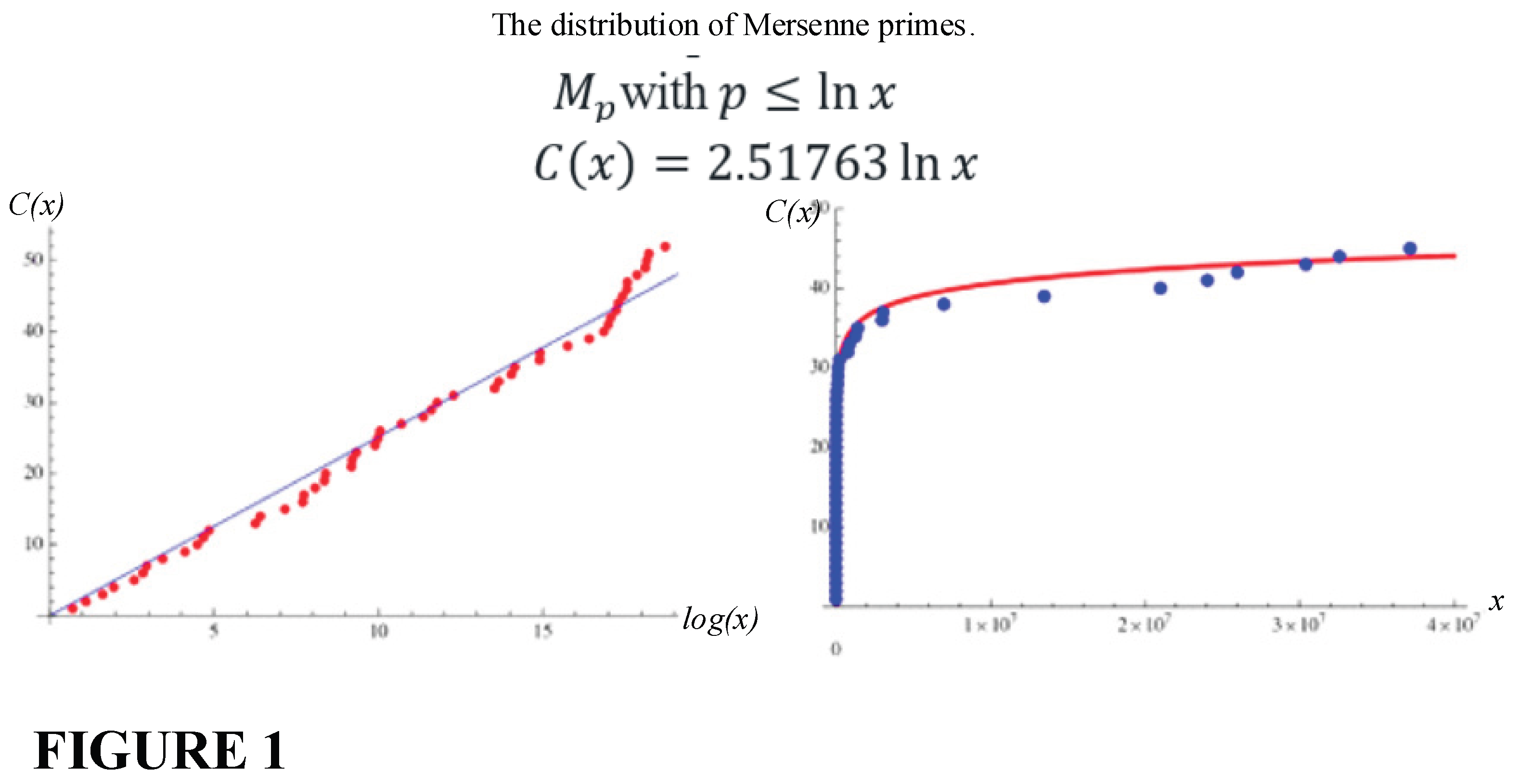
It is conjectured that there exist an infinite number of Mersenne primes. In Wolfram, we find the best fit line through the origin to the asymptotic number of Mersenne primes $M_p$with $p\le \ln x,$ for the first 51 known Mersenne primes. The best-fit line gives $C\left(x\right)=2.51763\ln x .$ This fit is illustrated below in Figures 1 & 2. It has been conjectured without any particularly strong evidence, that the constant is given by $e^{\lambda }\sqrt{2}=2.518..$, where $\lambda$ is the Euler-Mascheroni constant.

In this paper, I will give strong relations for this constant.

Figure 1 shows the asymptotic number of Mersenne primes $M_p$with $p\le \ln x, \left[5\right].$

Literature on Mersenne primes is mainly dedicated to the search for new Mersenne primes, and very few attempts have made progress on the actual theoretical work. In [8], Zhaodong Cai, Matthew Faust, A.J. Hildebrand, Junxian Li, and Yuan Zhang studied theleading digits of the Mersenne primes. They attempted to show that leading digits of Mersenne numbers behave in many respects more regularly than some sequences of powers of logs of 2. Further information on Perfect numbers, abondant numbers, and deficient numbers can be found in [7]. Reference [8] by the present author gives some resources on the Gamma function and its invariance. Most of the research in this paper is related to the present work only in an attempt to categorize properties that Mersenne primes may have found to have, however, the present paper does not rely on any of the current work known on Mersenne primes, but starts a new trend in exploring the properties of Mersenne primes. To begin, let us explore the concepts that lead to the final proof.

3. The Invariance of the Gamma Function to Substitution $\mathit{\sigma }\left(\mathit{m}\right)\to \mathit{\sigma }\left(\mathit{m}+\mathit{j}\right)$

I first want to introduce the curious fact that any function with a relational product $\left\{n·y\right\},$can be represented by the Sums of Divisor function$, \sigma \left(m\right)$. Here is a simple example:

$$\log \left(n·y\right)=\log n+ \log y,$$

(6)

$\mathrm{T}\mathrm{h}\mathrm{e}\mathrm{n}, \mathrm{i}\mathrm{f}n·y=m,$ we can put $n=\sigma \left(m\right), y={\displaystyle \frac{m}{\sigma \left(m\right)}},$ and so,

$$\log \left(m\right)=\log \sigma \left(m\right)+\log {\displaystyle \frac{m}{\sigma \left(m\right)}}$$

(7)

$\mathrm{T}\mathrm{h}\mathrm{e}\mathrm{n}, \mathrm{i}\mathrm{f}n·y={ N}_p,$ we can put $n=\sigma \left({ N}_p\right), y={\displaystyle \frac{{ N}_p}{\sigma \left({ N}_p\right)}},$ then, a Perfect number${ N}_p,$ has the relation:

$$\log \left({ N}_p\right)=\log \left(\sigma \left({ N}_p\right)\right)+ \log \left({\displaystyle \frac{{ N}_p}{\sigma \left({ N}_p\right)}}\right)$$

(8)

$$\log \left({ N}_p\right)=\log \left(\sigma \left({ N}_p\right)\right)+\log \left({\displaystyle \frac{1}{2}}\right)$$

(9)

Here is another example:

I$\mathrm{f} n·y=m,$ we can put $n=\sigma \left(m\right), y={\displaystyle \frac{m}{\sigma \left(m\right)}},$ and so, applied to the formula [3], p.41:

$$\begin{array}{c}\sin \left(n·x\right)=n\sin \left(x\right)\cos \left(x\right){\displaystyle \prod _{k=1}^{{\displaystyle \frac{n-2}{2}}}}\left(1-{\displaystyle \frac{{\sin }^2\left(x\right)}{{\sin }^2\left(\frac{k\pi }{n}\right)}}\right)\\ \cos \left(n·x\right)={\displaystyle \prod _{k=1}^{{\displaystyle \frac{n}{2}}}}\left(1-{\displaystyle \frac{{\sin }^2\left(x\right)}{{\sin }^2\left(\frac{\left(2k-1\right)\pi }{2n}\right)}}\right)\end{array}, \left[n \mathrm{i}\mathrm{s}\mathrm{ }\mathrm{e}\mathrm{v}\mathrm{e}\mathrm{n}\right]$$

(10)

$$\begin{array}{c}\sin \left(n·x\right)=n\sin \left(x\right){\displaystyle \prod _{k=1}^{{\displaystyle \frac{n-1}{2}}}}\left(1-{\displaystyle \frac{{\sin }^2\left(x\right)}{{\sin }^2\left(\frac{k\pi }{n}\right)}}\right)\\ \cos \left(n·x\right)=\cos \left(x\right){\displaystyle \prod _{k=1}^{{\displaystyle \frac{n-1}{2}}}}\left(1-{\displaystyle \frac{{\sin }^2\left(x\right)}{{\sin }^2\left(\frac{\left(2k-1\right)\pi }{2n}\right)}}\right)\end{array}, \left[n \mathrm{i}\mathrm{s}\mathrm{ }\mathrm{o}\mathrm{d}\mathrm{d}\right]$$

(11)

Interestingly, $\left(10\right)\in even,$ and $\left(11\right)\in odd$, differentiates between odd and even values of $n.$ Since primes have $\sigma \left(p\right)=p+1,$an even number, and $p+1$ is always even except for the prime 2, the relations $\left(11\right)\in odd.$And does not apply to odd numbers. Since $\sigma \left(2\right)=3.$For example,

$$\cos \left(2\right)=\cos \left({\displaystyle \frac{2}{3}}\right)\prod _{k=1}^1\left(1-{\displaystyle \frac{{\sin }^2\left(\frac{2}{3}\right)}{{\sin }^2\frac{\left(2k-1\right)\pi }{6}}}\right), \left[\sigma \left(2\right) \mathrm{i}\mathrm{s}\mathrm{ }\mathrm{o}\mathrm{d}\mathrm{d}\right]$$

(12)

$$-0.4161468365\dots =0.7858872608..\left(1-{\displaystyle \frac{0.3823812134\dots }{0.2500000000}}\right)=-0.4161468365\dots$$

(13)

By using the sum of divisor function, for Perfect numbers, ${ N}_p,$ the even trigonometric relations $\left[\left(10\right), \left(11\right)\right]\in even,$ apply, but the relations, $\left[\left(12\right), \left(13\right)\right]\in odd$ do not apply, so we can put, $\sigma \left({ N}_p\right)=2{ N}_p$. The fact that the sum of divisor function $\sigma \left(m\right),$can be manipulated this way leads to some interesting formulas that can produce significant and unexpected results.

4. Application of the Trigonometric Function to Perfect Numbers

A Perfect Number $N_p,$ is defined as a number for which $\sigma \left(N_p\right)=2N_p.$ A list of some known Perfect numbers is

$N_p\in \left\{6,28,496,8128,33550336,\mathrm{8589869056,137438691328},\mathrm{2305843008139952128,2658455991569831744654692615953842176},\dots \right\}$

Hence for, example, in (10), putting $n=\sigma \left(j\right), (n even), x={\displaystyle \frac{1}{j}}:$ then, we have

$$\begin{array}{c}\sin \left({\displaystyle \frac{\sigma \left(j\right)}{j}}\right)=\sigma \left(j\right)\sin \left({\displaystyle \frac{1}{j}}\right)\cos \left({\displaystyle \frac{1}{j}}\right){\displaystyle \prod _{k=1}^{{\displaystyle \frac{\sigma \left(j\right)-2}{2}}}}\left(1-{\displaystyle \frac{{\sin }^2\left(\frac{1}{j}\right)}{{\sin }^2\left(\frac{k\pi }{\sigma \left(j\right)}\right)}}\right)\\ \cos \left({\displaystyle \frac{\sigma \left(j\right)}{j}}\right)={\displaystyle \prod _{k=1}^{{\displaystyle \frac{\sigma \left(j\right)}{2}}}}\left(1-{\displaystyle \frac{{\sin }^2\left(\frac{1}{j}\right)}{{\sin }^2\left(\frac{\left(2k-1\right)\pi }{2\sigma \left(j\right)}\right)}}\right)\end{array}, \left[\sigma \left(j\right) \mathrm{i}\mathrm{s}\mathrm{ }\mathrm{e}\mathrm{v}\mathrm{e}\mathrm{n}\right]$$

(14)

$$\tan \left({\displaystyle \frac{\sigma \left(j\right)}{j}}\right)={\displaystyle \frac{\sigma \left(j\right)\sin \left(\frac{1}{j}\right)\cos \left(\frac{1}{j}\right)\prod _{k=1}^{\frac{\sigma \left(j\right)-2}{2}}\left(1-\frac{{\sin }^2\left(\frac{1}{j}\right)}{{\sin }^2\left(\frac{k\pi }{\sigma \left(j\right)}\right)}\right)}{\prod _{k=1}^{\frac{\sigma \left(j\right)}{2}}\left(1-\frac{{\sin }^2\left(\frac{1}{j}\right)}{{\sin }^2\left(\frac{\left(2k-1\right)\pi }{2\sigma \left(j\right)}\right)}\right)}} \left[\sigma \left(j\right) \mathrm{i}\mathrm{s}\mathrm{ }\mathrm{e}\mathrm{v}\mathrm{e}\mathrm{n}\right]$$

(15)

Lemma 1.

The rational trigonometric functions$\mathit{sin}\left({\displaystyle \frac{\sigma \left(j\right)}{j}}\right),\mathit{cos}\left({\displaystyle \frac{\sigma \left(j\right)}{j}}\right)$

 determine $Perfect Numbers.$

Proof 

$$\sigma \left(j\right)=\left[{\displaystyle \frac{\tan \left(\frac{\sigma \left(j\right)}{j}\right)\prod _{k=1}^{\frac{\sigma \left(j\right)}{2}}\left(1-\frac{{\sin }^2\left(\frac{1}{j}\right)}{{\sin }^2\left(\frac{\left(2k-1\right)\pi }{2\sigma \left(j\right)}\right)}\right)}{ \sin \left(\frac{1}{j}\right)\cos \left(\frac{1}{j}\right)\prod _{k=1}^{\frac{\sigma \left(j\right)}{2}}\left(1-\frac{{\sin }^2\left(\frac{1}{j}\right)}{{\sin }^2\left(\frac{\left(2k-1\right)\pi }{2\sigma \left(j\right)}\right)}\right)}}\right]$$

(16)

$$\sigma \left(j\right)=2\left[{\displaystyle \frac{\tan \left(\frac{\sigma \left(j\right)}{j}\right)\prod _{k=1}^{\frac{\sigma \left(j\right)}{2}}\left(1-\frac{{\sin }^2\left(\frac{1}{j}\right)}{{\sin }^2\left(\frac{\left(2k-1\right)\pi }{2\sigma \left(j\right)}\right)}\right)}{2 \sin \left(\frac{1}{j}\right)\cos \left(\frac{1}{j}\right)\prod _{k=1}^{\frac{\sigma \left(j\right)}{2}}\left(1-\frac{{\sin }^2\left(\frac{1}{j}\right)}{{\sin }^2\left(\frac{\left(2k-1\right)\pi }{2\sigma \left(j\right)}\right)}\right)}}\right]$$

(17)

$$\sigma \left(j\right)=2\left[{\displaystyle \frac{\tan \left(\frac{\sigma \left(j\right)}{j}\right)\prod _{k=1}^{\frac{\sigma \left(j\right)}{2}}\left(1-\frac{{\sin }^2\left(\frac{1}{j}\right)}{{\sin }^2\left(\frac{\left(2k-1\right)\pi }{2\sigma \left(j\right)}\right)}\right)}{\sin \left(\frac{2}{j}\right)\prod _{k=1}^{\frac{\sigma \left(j\right)}{2}}\left(1-\frac{{\sin }^2\left(\frac{1}{j}\right)}{{\sin }^2\left(\frac{\left(2k-1\right)\pi }{2\sigma \left(j\right)}\right)}\right)}}\right]$$

(18)

If $j=$ $N_p$is a Perfect number, then, the equality applies only when.

$$N_p={\displaystyle \frac{\tan \left(\frac{\sigma \left(N_p\right)}{N_p}\right)\prod _{k=1}^{\frac{\sigma \left(N_p\right)}{2}}\left(1-\frac{{\sin }^2\left(\frac{1}{N_p}\right)}{{\sin }^2\left(\frac{\left(2k-1\right)\pi }{2\sigma \left(N_p\right)}\right)}\right)}{ \sin \left(\frac{2}{N_p}\right)\left(\prod _{k=1}^{\frac{\sigma \left(N_p\right)}{2}-1}\left(1-\frac{{\sin }^2\left(\frac{1}{N_p}\right)}{{\sin }^2\left(\frac{k\pi }{\sigma \left(N_p\right)}\right)}\right)\right)}}$$

(19)

Taking the limits:

$$\underset{N_p\to \infty }{\lim }{N}_p=\underset{N_p\to \infty }{\lim }\left(\tan \left(2\right)\left\{{\displaystyle \frac{\prod _{k=1}^{\frac{\sigma \left(N_p\right)}{2}}\left(1-\frac{{\sin }^2\left(\frac{1}{N_p}\right)}{{\sin }^2\left(\frac{\left(2k-1\right)\pi }{2\sigma \left(N_p\right)}\right)}\right)}{ \sin \left(\frac{2}{N_p}\right)\left(\prod _{k=1}^{\frac{\sigma \left(N_p\right)}{2}-1}\left(1-\frac{{\sin }^2\left(\frac{1}{N_p}\right)}{{\sin }^2\left(\frac{k\pi }{\sigma \left(N_p\right)}\right)}\right)\right)}}\right\}\right)$$

(20)

Now, for large values of$y,$ $\sin \left({\displaystyle \frac{1}{y}}\right)\to {\displaystyle \frac{1}{y}},$ and so we can approximate the product for large values of $N_p$as follows:

$$\underset{N_p\to \infty }{\lim }{N}_p=\underset{N_p\to \infty }{\mathrm{l}\mathrm{i}\mathrm{m}}\left({\displaystyle \frac{\tan \left(2\right)}{\sin \left(\frac{2}{N_p}\right)}}\left(1-{\left({\displaystyle \frac{2\sigma \left(N_p\right)}{N_p\left(\sigma \left(N_p\right)-1\right)\pi }}\right)}^2\right)\left\{\prod _{k=1}^{{\displaystyle \frac{\sigma \left(N_p\right)}{2}}-1}{\displaystyle \frac{\left(1-{\left(\frac{2\sigma \left(N_p\right)}{N_p\left(2k-1\right)\pi }\right)}^2\right)}{\left(1-{\left(\frac{\sigma \left(N_p\right)}{N_{p}k\pi }\right)}^2\right)}}\right\}\right)$$

(21)

$$\underset{N_p\to \infty }{\lim }{N}_p=\underset{N_p\to \infty }{\mathrm{l}\mathrm{i}\mathrm{m}}\left(N_p{\displaystyle \frac{\tan \left(2\right)}{2}}\left\{\prod _{k=1}^{{\displaystyle \frac{\sigma \left(N_p\right)}{2}}-1}{\displaystyle \frac{\left(1-{\left(\frac{2\sigma \left(N_p\right)}{N_p\left(2k-1\right)\pi }\right)}^2\right)}{\left(1-{\left(\frac{\sigma \left(N_p\right)}{N_{p}k\pi }\right)}^2\right)}}\right\}\right)$$

(22)

$$1={\displaystyle \frac{\tan \left(2\right)}{2}}\left\{\prod _{k=1}^{\infty }{\displaystyle \frac{\left(1-\frac{4{\left(x\right)}^2}{{\left(2k-1\right)}^2{\pi }^2}\right)}{\left(1-\frac{{\left(x\right)}^2}{k^2{\pi }^2}\right)}}\right\}$$

(23)

For the infinite product we have,

$$\sin \left(nx\right)=n\sin \left(x\right)\cos \left(x\right)\prod _{k=1}^{{\displaystyle \frac{n-2}{2}}}\left(1-{\displaystyle \frac{{\sin }^2\left(x\right)}{{\sin }^2\left(\frac{k\pi }{n}\right)}}\right)$$

(24)

$$\cos \left(nx\right)=\prod _{k=1}^{{\displaystyle \frac{n}{2}}}\left(1-{\displaystyle \frac{{\sin }^2\left(x\right)}{{\sin }^2\left(\frac{\left(2k-1\right)\pi }{2n}\right)}}\right)$$

(25)

Put,$n=\sigma \left(N_p\right)$ $, x={\displaystyle \frac{1}{N_p}},$

$$\begin{array}{c}\sin \left({\displaystyle \frac{\sigma \left(N_p\right)}{N_p}}\right)=\sigma \left(N_p\right)\sin \left({\displaystyle \frac{1}{N_p}}\right)\cos \left({\displaystyle \frac{1}{N_p}}\right){\displaystyle \prod _{k=1}^{{\displaystyle \frac{\sigma \left(N_p\right)-2}{2}}}}\left(1-{\displaystyle \frac{{\sin }^2\left(\frac{1}{N_p}\right)}{{\sin }^2\left(\frac{k\pi }{\sigma \left(N_p\right)}\right)}}\right)\\ \cos \left({\displaystyle \frac{\sigma \left(N_p\right)}{N_p}}\right)={\displaystyle \prod _{k=1}^{{\displaystyle \frac{\sigma \left(N_p\right)}{2}}}}\left(1-{\displaystyle \frac{{\sin }^2\left(\frac{1}{N_p}\right)}{{\sin }^2\left(\frac{\left(2k-1\right)\pi }{2\sigma \left(N_p\right)}\right)}}\right)\end{array}, \left[\sigma \left(N_p\right) \mathrm{i}\mathrm{s}\mathrm{ }\mathrm{e}\mathrm{v}\mathrm{e}\mathrm{n}\right]$$

(26)

It is clear that there if there exists a continued set of infinitely large Perfect Numbers then,

$$\left.\begin{array}{c}\sin \left(2\right)-\sigma \left(N_p\right)\sin \left({\displaystyle \frac{1}{N_p}}\right)\cos \left({\displaystyle \frac{1}{N_p}}\right){\displaystyle \prod _{k=1}^{{\displaystyle \frac{\sigma \left(N_p\right)-2}{2}}}}\left(1-{\displaystyle \frac{{\sin }^2\left(\frac{1}{N_p}\right)}{{\sin }^2\left(\frac{k\pi }{\sigma \left(N_p\right)}\right)}}\right)\\ \begin{array}{c}\cos \left(2\right)-{\displaystyle \prod _{k=1}^{{\displaystyle \frac{\sigma \left(N_p\right)}{2}}}}\left(1-{\displaystyle \frac{{\sin }^2\left(\frac{1}{N_p}\right)}{{\sin }^2\left(\frac{\left(2k-1\right)\pi }{2\sigma \left(N_p\right)}\right)}}\right)\\ N_p-\tan \left(2\right){\displaystyle \frac{\prod _{k=1}^{\frac{\sigma \left(N_p\right)}{2}}\left(1-\frac{{\sin }^2\left(\frac{1}{N_p}\right)}{{\sin }^2\left(\frac{\left(2k-1\right)\pi }{2\sigma \left(N_p\right)}\right)}\right)}{ \sin \left(\frac{2}{N_p}\right)\left(\prod _{k=1}^{\frac{\sigma \left(N_p\right)}{2}-1}\left(1-\frac{{\sin }^2\left(\frac{1}{N_p}\right)}{{\sin }^2\left(\frac{k\pi }{\sigma \left(N_p\right)}\right)}\right)\right)}}\end{array}\end{array}\right\}=0, \begin{array}{c}\left[\sigma \left(N_p\right) \mathrm{i}\mathrm{s}\mathrm{ }\mathrm{e}\mathrm{v}\mathrm{e}\mathrm{n}\right], \left(\models \right) for n\in N_p\\ otherwise for n\notin N_p\end{array}$$

(27)

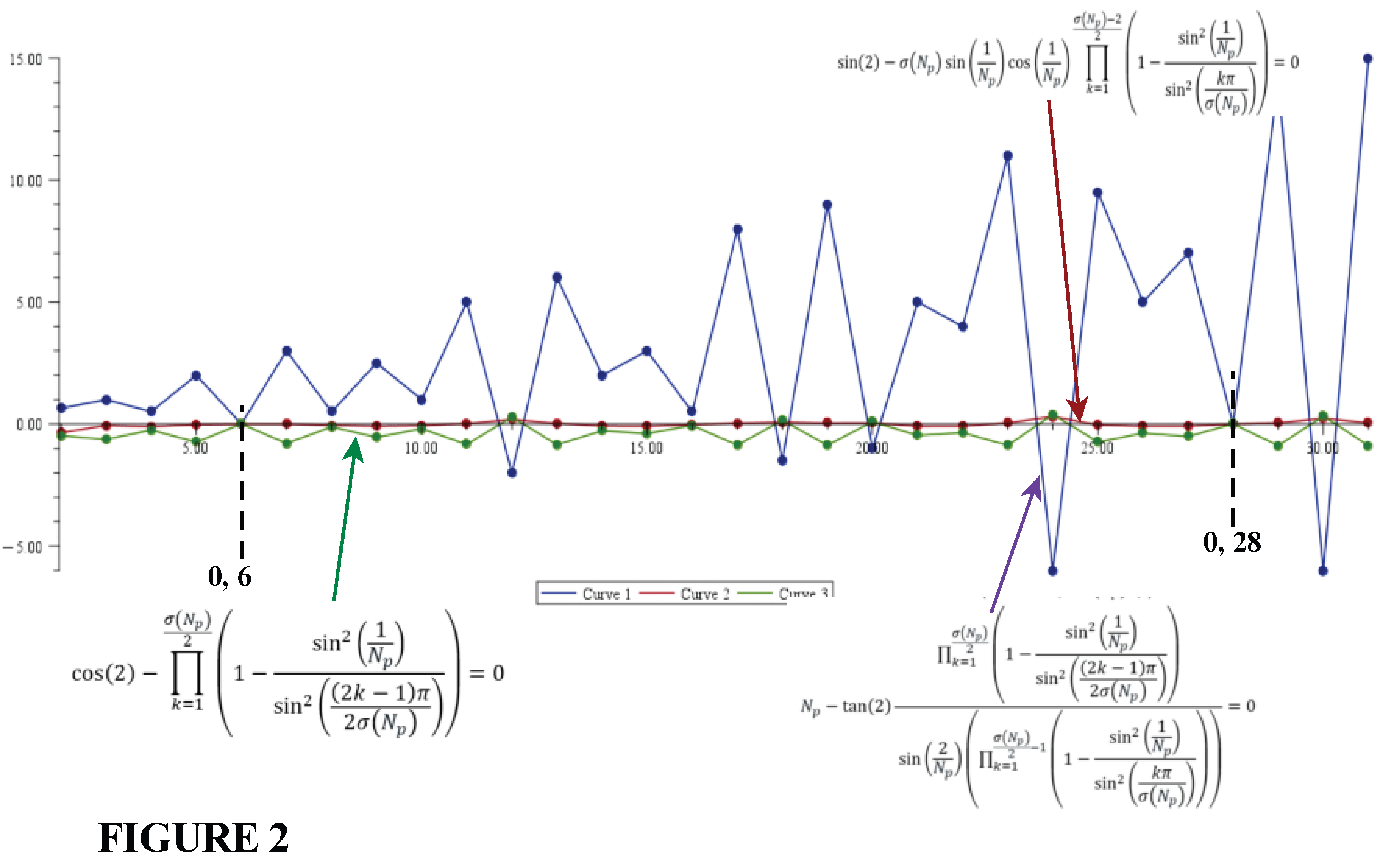
Each of these three relations is only true when $N_p$ is a Perfect number.

Figure 2 shows the correletion of the relation (27) with Perfect Numbers.

From symmetry, and considering the form for the divisor function:

$$N_p={\displaystyle \frac{\tan \left(2\right)\prod _{k=1}^{N_p}\left(1-\frac{{\sin }^2\left(\frac{1}{N_p}\right)}{{\sin }^2\left(\frac{\left(2k-1\right)\pi }{4N_p}\right)}\right)}{ \sin \left(\frac{2}{N_p}\right)\left(\prod _{k=1}^{N_p-1}\left(1-\frac{{\sin }^2\left(\frac{1}{N_p}\right)}{{\sin }^2\left(\frac{k\pi }{2N_p}\right)}\right)\right)}}$$

(28)

Since $N_p=\left(2^p-1\right)2^{p-1}$, where $p$ is a prime, we can factor the perfect number $N_p,$as follows:

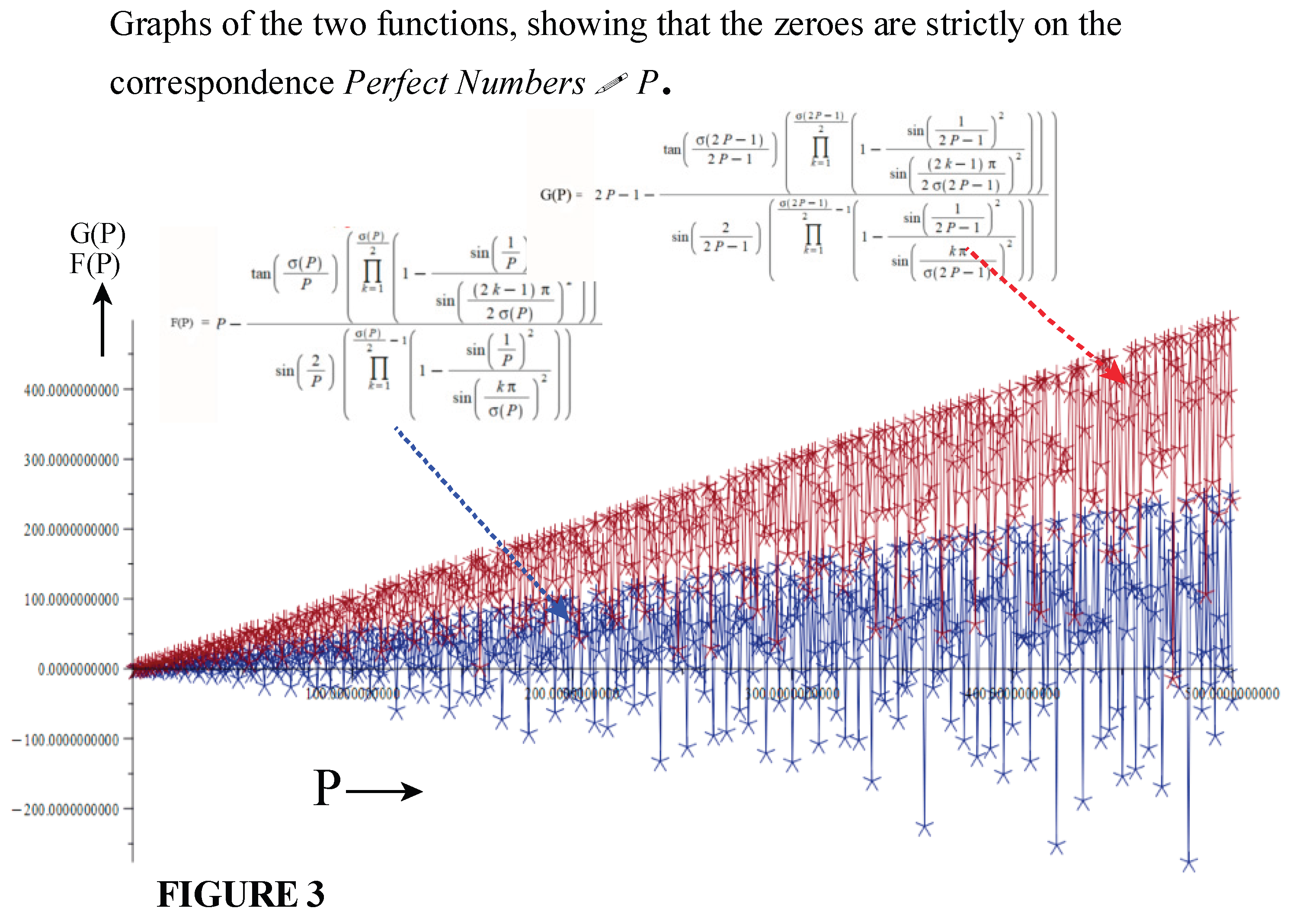
$N_p=\left(2^p-1\right)2^{p-1}=\left(2P-1\right)P$, where $P=2^{p-1}.$ This factorization leads to the following results:

$$\begin{array}{c}F\left(P\right)=P-{\displaystyle \frac{\tan \left(\frac{\sigma \left(P\right)}{P}\right)\prod _{k=1}^{\frac{\sigma \left(P\right)}{2}}\left(1-\frac{{\sin }^2\left(\frac{1}{P}\right)}{{\sin }^2\left(\frac{\left(2k-1\right)\pi }{2\sigma \left(P\right)}\right)}\right)}{ \sin \left(\frac{2}{P}\right)\left(\prod _{k=1}^{\frac{\sigma \left(P\right)}{2}-1}\left(1-\frac{{\sin }^2\left(\frac{1}{P}\right)}{{\sin }^2\left(\frac{k\pi }{\sigma \left(P\right)}\right)}\right)\right)}}\\ G\left(P\right)=2P-1-{\displaystyle \frac{\tan \left(\frac{\sigma \left(2P-1\right)}{2P-1}\right)\prod _{k=1}^{\frac{\sigma \left(2P-1\right)}{2}}\left(1-\frac{{\sin }^2\left(\frac{1}{2P-1}\right)}{{\sin }^2\left(\frac{\left(2k-1\right)\pi }{2\sigma \left(2P-1\right)}\right)}\right)}{ \sin \left(\frac{2}{2P-1}\right)\left(\prod _{k=1}^{\frac{\sigma \left(2P-1\right)}{2}-1}\left(1-\frac{{\sin }^2\left(\frac{1}{P}\right)}{{\sin }^2\left(\frac{k\pi }{\sigma \left(2P-1\right)}\right)}\right)\right)}}\end{array}$$

(29)

It is clear that the there is a direct correspondence between the Perfect Number $N_p,$and $P.$ The graphs of the two functions is shown in Figure 3.

$$F\left(P\right)=P-{\displaystyle \frac{\tan \left(\frac{\sigma \left(P\right)}{P}\right)\prod _{k=1}^{\frac{\sigma \left(P\right)}{2}}\left(1-\frac{{\sin }^2\left(\frac{1}{P}\right)}{{\sin }^2\left(\frac{\left(2k-1\right)\pi }{2\sigma \left(P\right)}\right)}\right)}{ \sin \left(\frac{2}{P}\right)\left(\prod _{k=1}^{\frac{\sigma \left(P\right)}{2}-1}\left(1-\frac{{\sin }^2\left(\frac{1}{P}\right)}{{\sin }^2\left(\frac{k\pi }{\sigma \left(P\right)}\right)}\right)\right)}}$$

(30)

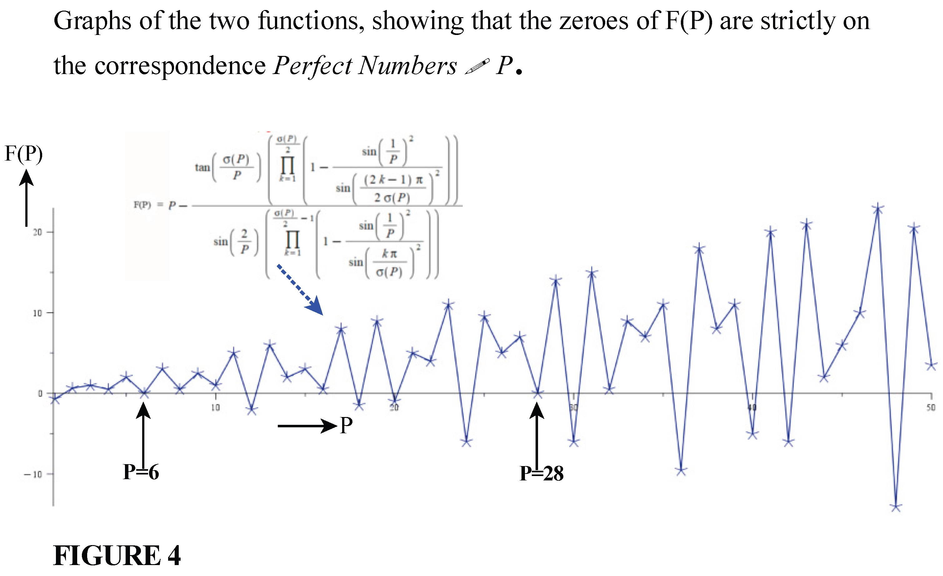
Figure 4 shows the correspondence $F\left(P\right)\to N_p.$

The relations (19) hold for all Perfect Numbers. The right hand side of (19) does not depend on implicit rational relationships between $\sigma \left(N_p\right)$ and $N_p.$ It is clear that the basic rational trigonometric functions capture the properties of Perfgect numbers, and hence Mersenne primes. We now explore the general forms of trinometric and exponential forms that capture Perfect numbers, Abondant numbers and deficient numbers in one relation.

5. The General Relation That Captures the Behavior of Abondant Numbers, Perfect Numbers and Deficient Numbers

Definition 1.

An Abundant number is a positive integer for which the sum of its proper divisors excluding itself is greater than the number itself.

Definition 2.

A Perfect number is a number for which the sums of all divisors is equal to twice the number.

Definition 3.

A Deficient number is a number for which the sums of all divisors is less than twice the number.

Lemma. 

If$n$

 is a Perfect number, then,

$${\displaystyle \frac{\cos \left(\frac{2\pi n}{\sigma \left(n\right)}\right)}{\sin \left(\frac{\pi n}{\sigma \left(n\right)}\right)}}=-1$$

(31)

Proof. 

for a Perfect number, $\sigma \left(n\right)=2n.$

Hence,

$${\displaystyle \frac{\cos \left(\pi \right)}{\sin \left(\frac{\pi }{2}\right)}}=-1$$

(32)

The distribution of perfect numbers, abondant numbers and deficient numbers is captured by the general relation:

$$\cos \left({\displaystyle \frac{2n\pi }{\sigma \left(n\right)}}\right)+\sin \left({\displaystyle \frac{n\pi }{\sigma \left(n\right)}}\right)=0$$

(33)

For perfect numbers, ${\displaystyle \frac{2n}{\sigma \left(n\right)}}=1,$and the relation (33) vanishes.

For abondant numbers, ${\displaystyle \frac{2n}{\sigma \left(n\right)}}<1,$and the relation does not vanish but generates negetaive imaginary values for $n\in \mathbf{a}\mathbf{b}\mathbf{o}\mathbf{n}\mathbf{d}\mathbf{a}\mathbf{n}\mathbf{t} \mathbf{n}\mathbf{u}\mathbf{m}\mathbf{b}\mathbf{e}\mathbf{r}\mathbf{s}.$For deficient numbers, ${\displaystyle \frac{2n}{\sigma \left(n\right)}}<1,$and the relation does not vanish but generates positive imaginary values for $n\in \mathbf{d}\mathbf{e}\mathbf{f}\mathbf{i}\mathbf{c}\mathbf{i}\mathbf{e}\mathbf{n}\mathbf{t} \mathbf{n}\mathbf{u}\mathbf{m}\mathbf{b}\mathbf{e}\mathbf{r}\mathbf{s}.$To see this, put the relation (33) in the form:

$${\displaystyle \frac{\cos \left(\frac{2n\pi }{\sigma \left(n\right)}\right)}{\sin \left(\frac{n\pi }{\sigma \left(n\right)}\right)}}=-1 \sin \left({\displaystyle \frac{n\pi }{\sigma \left(n\right)}}\right)\ne 0,$$

(34)

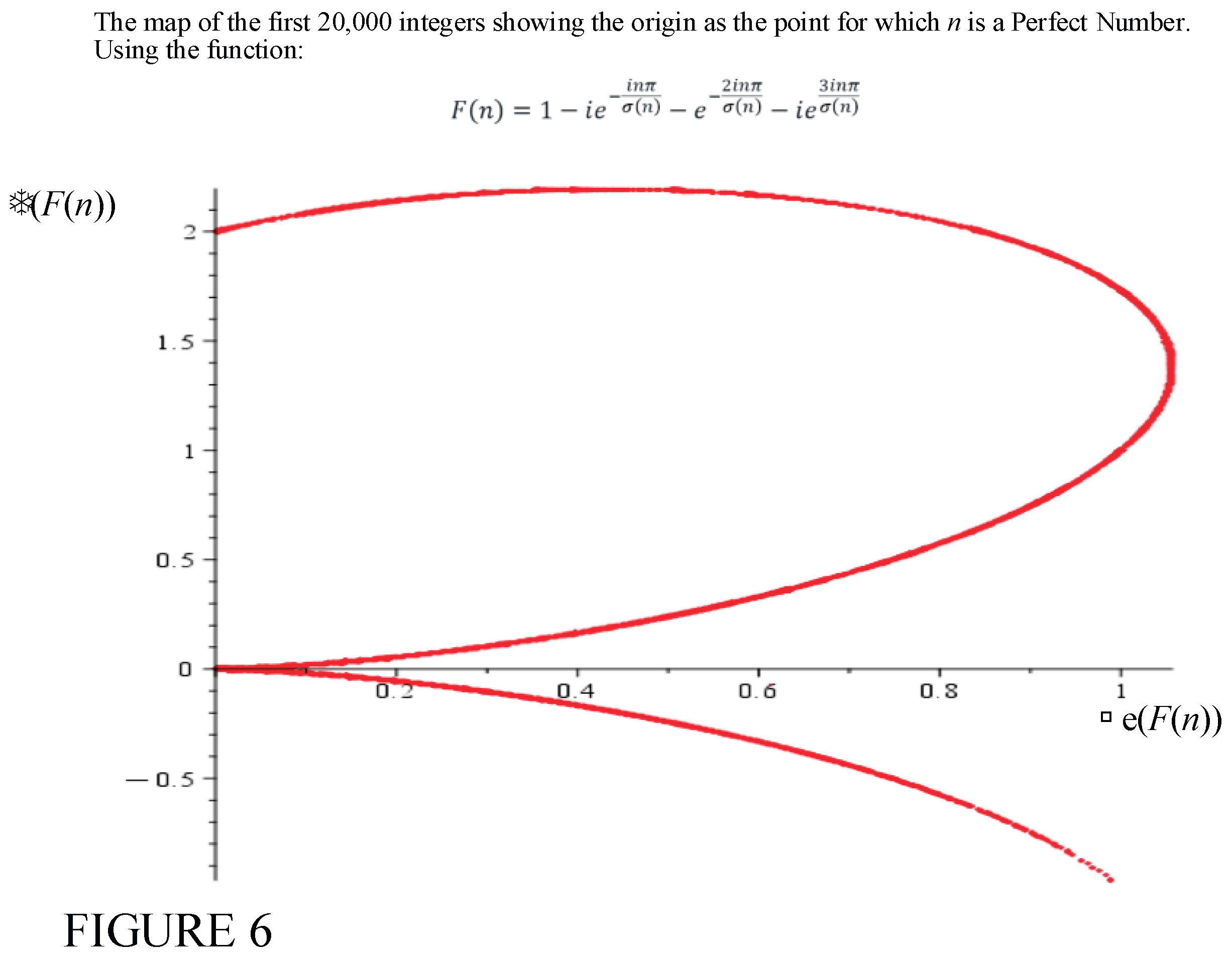
Obviously, the zeros of the function (34) occur at the Perfect numbers. However, for clarity we convert this relation to the exponential form:

$$F\left(n\right)=1-i{e}^{-{\displaystyle \frac{in\pi }{\sigma \left(n\right)}}}-e^{-{\displaystyle \frac{2in\pi }{\sigma \left(n\right)}}}-i{e}^{{\displaystyle \frac{3in\pi }{\sigma \left(n\right)}}}$$

(35)

Figure 6 shows the complex map of the function $F\left(n\right),$ over the range $n=0..\mathrm{20,000}$.

The zeros of the function $F\left(n\right),$ occur at the values 6, 28, 496, 8124….

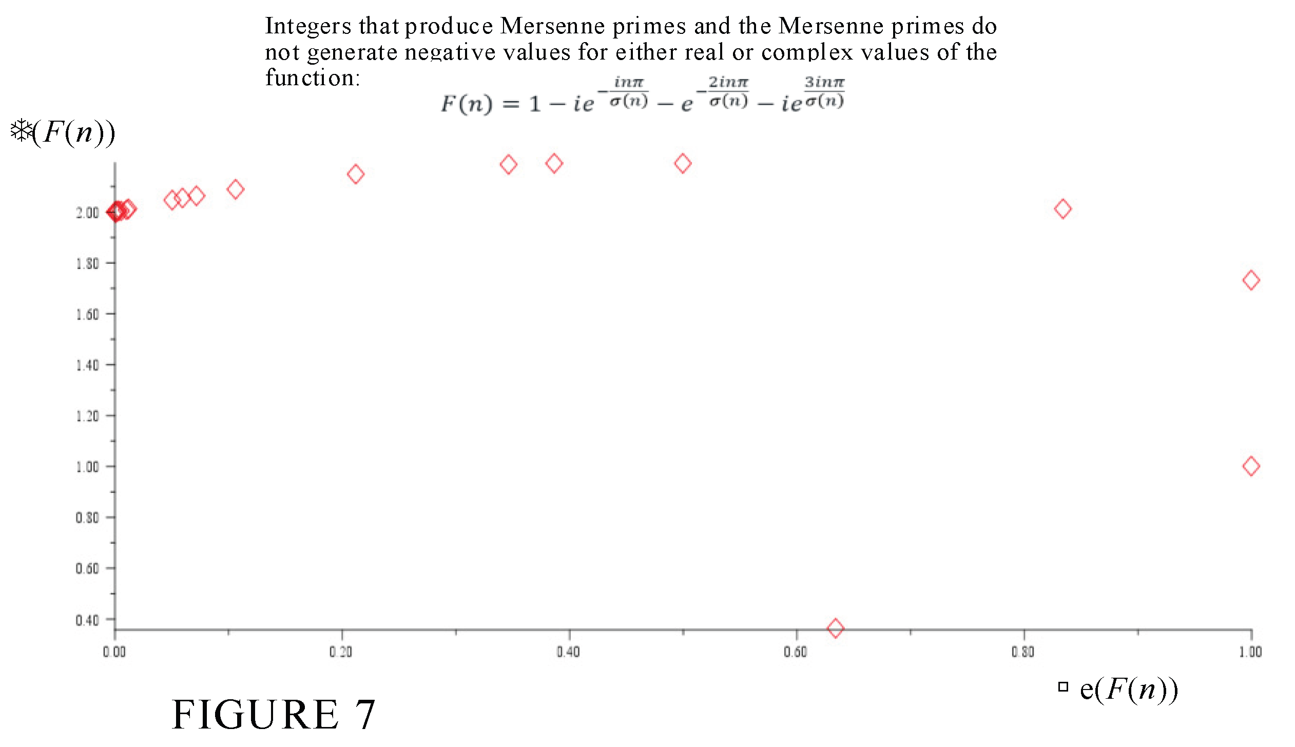
NOTE*: The Mersenne primes and the perfect numbers can only exist on the upper right quadrant corrsponding to deficient numbers. Perfect numbers are the zeros of the function $F\left(n\right)$.

The general locations of primes and Mersenne primes are shown in Figure 7. As can be seen, the oprimes do not generate negative imaginary values, and are located on the top-right quadrant of the complex plane.

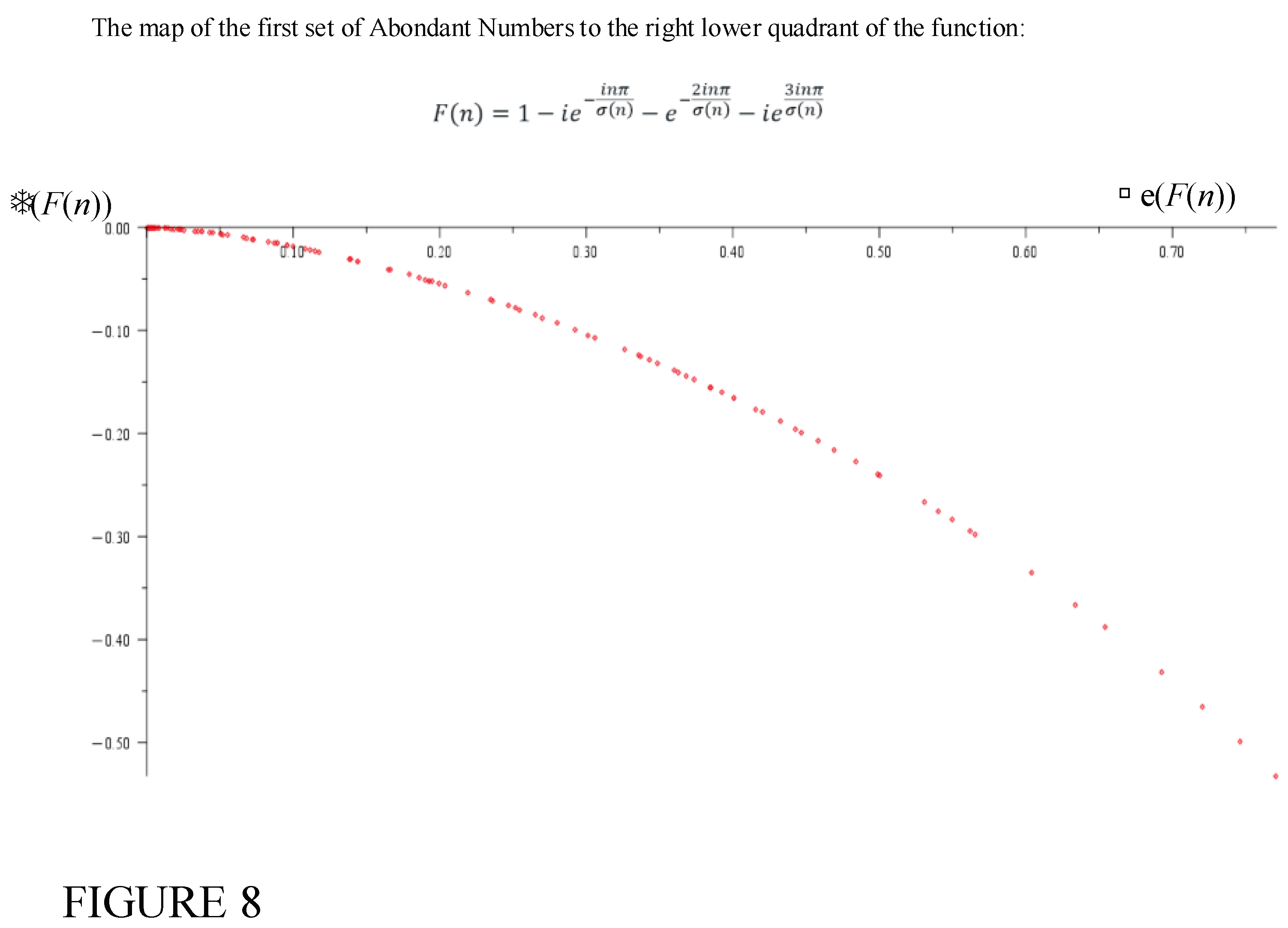
Hence, $\sigma \left(n\right)>2n.$ It is clear that the sequence of abundant numbers,

[12, 18, 20, 24, 30, 36, 40, 42, 48, 54, 56, 60, 66, 70, 72, 78, 80, 84, 88, 90, 96, 100, 102, 104, 108, 112, 114, 120, 126, 132, 138, 140, 144, 150, 156, 160, 162, 168, 174, 176, 180, 186, 192, 196, 198, 200, 204, 208, 210, 216, 220, 222, 224, 228, 234, 240, 246, 252, 258, 260, 264, 270, 272, 276, 280, 282, 288, 294, 300, 304, 306, 308, 312, 318, 320, 324, 330, 336, 340, 342, 348, 350, 352, 354, 360, 364, 366, 368, 372, 378, 380, 384, 390, 392, 396, 400, 402, 408, 414, 416, 420, 426, 432, 438, 440, 444, 448, 450, 456, 460, 462, 464, 468, 474, 476, 480, 486, 490, 492, 498, 500],

produce values of $F\left(n\right)$ in (35) that lie on the lower right quadrant of the complex plane. This distinct observation for the first 500, abondant numbers provides a clue as to their distribution.

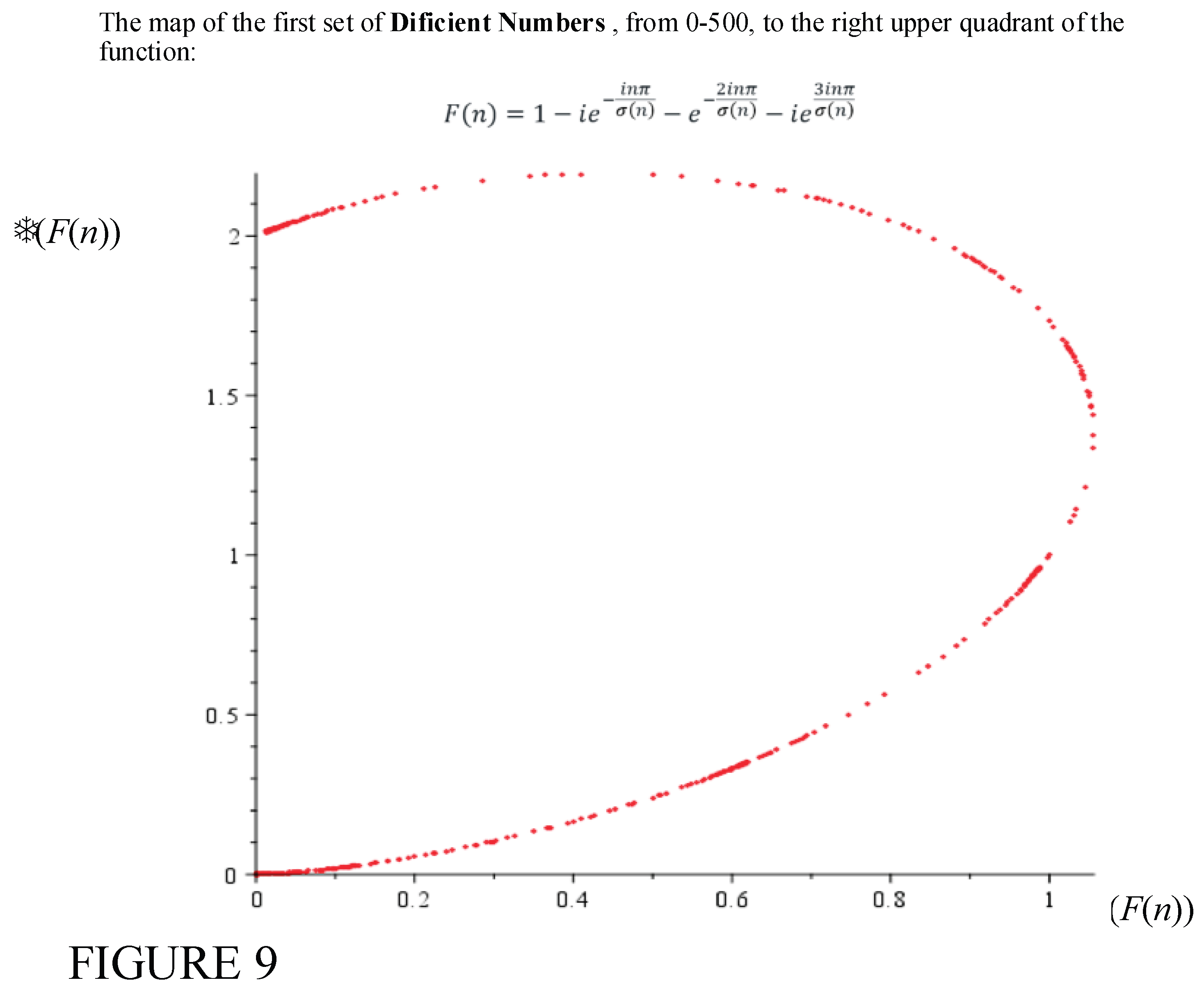
It is clear the first numbers between 0 and 500 that generate a sequence of deficient numbers:

[2, 3, 4, 5, 7, 8, 9, 10, 11, 13, 14, 15, 16, 17, 19, 21, 22, 23, 25, 26, 27, 29, 31, 32, 33, 34, 35, 37, 38, 39, 41, 43, 44, 45, 46, 47, 49, 50, 51, 52, 53, 55, 57, 58, 59, 61, 62, 63, 64, 65, 67, 68, 69, 71, 73, 74, 75, 76, 77, 79, 81, 82, 83, 85, 86, 87, 89, 91, 92, 93, 94, 95, 97, 98, 99, 101, 103, 105, 106, 107, 109, 110, 111, 113, 115, 116, 117, 118, 119, 121, 122, 123, 124, 125, 127, 128, 129, 130, 131, 133, 134, 135, 136, 137, 139, 141, 142, 143, 145, 146, 147, 148, 149, 151, 152, 153, 154, 155, 157, 158, 159, 161, 163, 164, 165, 166, 167, 169, 170, 171, 172, 173, 175, 177, 178, 179, 181, 182, 183, 184, 185, 187, 188, 189, 190, 191, 193, 194, 195, 197, 199, 201, 202, 203, 205, 206, 207, 209, 211, 212, 213, 214, 215, 217, 218, 219, 221, 223, 225, 226, 227, 229, 230, 231, 232, 233, 235, 236, 237, 238, 239, 241, 242, 243, 244, 245, 247, 248, 249, 250, 251, 253, 254, 255, 256, 257, 259, 261, 262, 263, 265, 266, 267, 268, 269, 271, 273, 274, 275, 277, 278, 279, 281, 283, 284, 285, 286, 287, 289, 290, 291, 292, 293, 295, 296, 297, 298, 299, 301, 302, 303, 305, 307, 309, 310, 311, 313, 314, 315, 316, 317, 319, 321, 322, 323, 325, 326, 327, 328, 329, 331, 332, 333, 334, 335, 337, 338, 339, 341, 343, 344, 345, 346, 347, 349, 351, 353, 355, 356, 357, 358, 359, 361, 362, 363, 365, 367, 369, 370, 371, 373, 374, 375, 376, 377, 379, 381, 382, 383, 385, 386, 387, 388, 389, 391, 393, 394, 395, 397, 398, 399, 401, 403, 404, 405, 406, 407, 409, 410, 411, 412, 413, 415, 417, 418, 419, 421, 422, 423, 424, 425, 427, 428, 429, 430, 431, 433, 434, 435, 436, 437, 439, 441, 442, 443, 445, 446, 447, 449, 451, 452, 453, 454, 455, 457, 458, 459, 461, 463, 465, 466, 467, 469, 470, 471, 472, 473, 475, 477, 478, 479, 481, 482, 483, 484, 485, 487, 488, 489, 491, 493, 494, 495, 497, 499 ],

produce values of $F\left(n\right)$ that lie on the upper right quadrant of the complex plane. This distinct observation for the first 500, defficient numbers and abondant numbers provides a clue as to their distributions.

Between the abondant numbers and the deficient numbers, are the Perfect Numbers, [6, 7, 28, 496, 8128, 33550336,….], that generate the zeros of the function:

$$F\left(n\right)=1-i{e}^{-{\displaystyle \frac{in\pi }{\sigma \left(n\right)}}}-e^{-{\displaystyle \frac{2in\pi }{\sigma \left(n\right)}}}-i{e}^{{\displaystyle \frac{3in\pi }{\sigma \left(n\right)}}} =0.$$

(36)

Hence, the imaginary part of the function $F\left(n\right)$ determines if a number is an abondant number, a perfect number or a deficient number.

$$\mathfrak{I}\left(1-i{e}^{-{\displaystyle \frac{in\pi }{\sigma \left(n\right)}}}-e^{-{\displaystyle \frac{2in\pi }{\sigma \left(n\right)}}}-i{e}^{{\displaystyle \frac{3in\pi }{\sigma \left(n\right)}}}\right)\begin{array}{c} <0, \\ =0, \\ >0, \end{array} \begin{array}{c}n\in abondant numbers \\ n\in perfect numbers \\ n\in deficient numbers\end{array}$$

(37)

The first set of even numbers from 0..500 that lie on the defient number curve but are not abondant numbers are:

[2, 4, 6, 8, 10, 14, 16, 22, 26, 28, 32, 34, 38, 44, 46, 50, 52, 58, 62, 64, 68, 72, 74, 76, 82, 86, 92, 94, 98, 106, 110, 116, 118, 122, 124, 128, 130, 134, 136, 142, 146, 148, 152, 154, 158, 164, 166, 170, 172, 178, 182, 184, 188, 190, 194, 202, 206, 212, 214, 218, 226, 230, 232, 236, 238, 242, 244, 248, 250, 254, 256, 262, 266, 268, 274, 278, 284, 286, 290, 292, 296, 298, 302, 304, 310, 314, 316, 322, 326, 328, 332, 334, 338, 344, 346, 356, 358, 362, 370, 374, 376, 382, 386, 388, 394, 398, 404, 406, 410, 412, 418, 422, 424, 428, 430, 434, 436, 442, 446, 452, 454, 458, 466, 470, 472, 478, 482, 484, 488, 494, 496].

These numbers are clearly defined by (37).

Figure 10 shows the 2D plot of the function covering both odd and even numbers in the range $n=0 ..50$0.

It is clear that the even numbers (red points) can fall on both the deficient number curve and the abondant number curve. The deficient numbers seem to be bounded by the line $1.05629905839783049963+1.37659573355141432857i$ and a maximum imaginary value of $0.43293432010231995809+2.19494797760015472936i$.

Definition 4: An Deficient disturbing number , (DDN), is a deficient number which:

$$\mathfrak{I}\left(1-i{e}^{-{\displaystyle \frac{in\pi }{\sigma \left(n\right)}}}-e^{-{\displaystyle \frac{2in\pi }{\sigma \left(n\right)}}}-i{e}^{{\displaystyle \frac{3in\pi }{\sigma \left(n\right)}}}\right)>0 \in \mathit{D}\mathit{D}\mathit{N}$$

(38)

These are the red points on Figure 10 that intermingle with the blue odd number points.

$DDN\in$ [2,4,8,10,14,16,22,26,32,34,38,44,46,50,52,58,62,64,68,74,76,82,86,92,94,98,106,110,116,118,122,124,128,130,134,136,142,146,148,152,154,158,164,166,170,172,178,182,184,188,190,194,202,206,212,214,218,226,230,232,236,238,242,244,248,250,254,256,262,266,268,274,278,284,286,290,292,296,298,302,310,314,316,322,326,328,332,334,338,344,346,356,358,362,370,374,376,382,386,388,394,398,404,406,410,412,418,422,424,428,430,434,436,442,446,452,454,458,466,470,472,478,482,484,488,494…..].

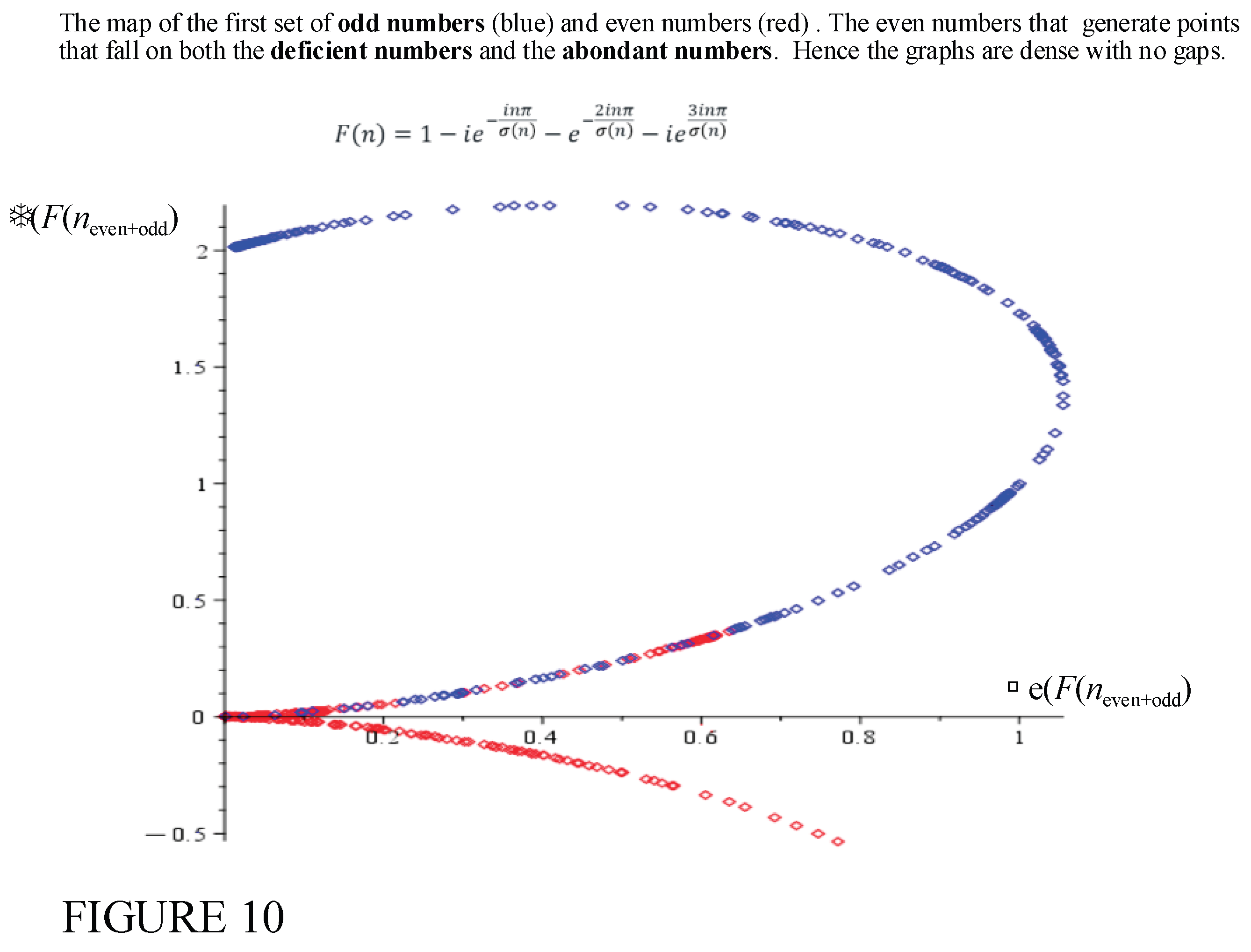
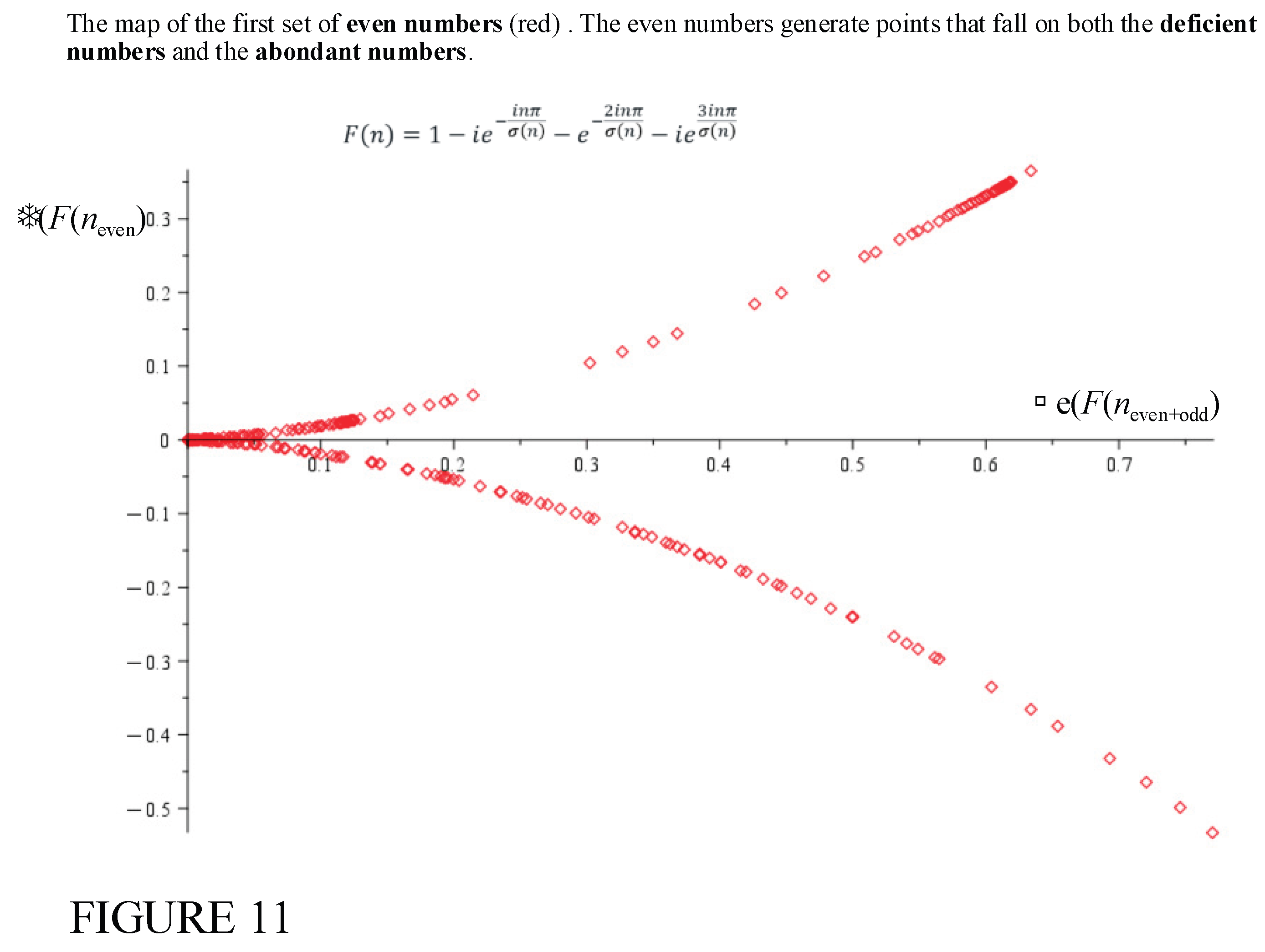
The extent to which the even numbers infiltrate the deficient number space for up to $n= 150000$ seems to be confined to the approximate range,

$$0 \le \left(1-i{e}^{-{\displaystyle \frac{in\pi }{\sigma \left(n\right)}}}-e^{-{\displaystyle \frac{2in\pi }{\sigma \left(n\right)}}}-i{e}^{{\displaystyle \frac{3in\pi }{\sigma \left(n\right)}}}\right)\le 0.98575151303581662431+0.36599952081502975396i , \mathit{D}\mathit{D}\mathit{N}\le 150000$$

(39)

The extent to which the even numbers penetrate the abondant number space is unknown. However it is known that there exists in infinite number of abundant numbers. It has been shown that every multiple $6(n\ge 6)$ is either an abondant number, or taking more multiples of 6 of such numbers leads to an bondant number. Since there is an infinite number of multiples of 6, then there are an infinite number of abondant numbers.

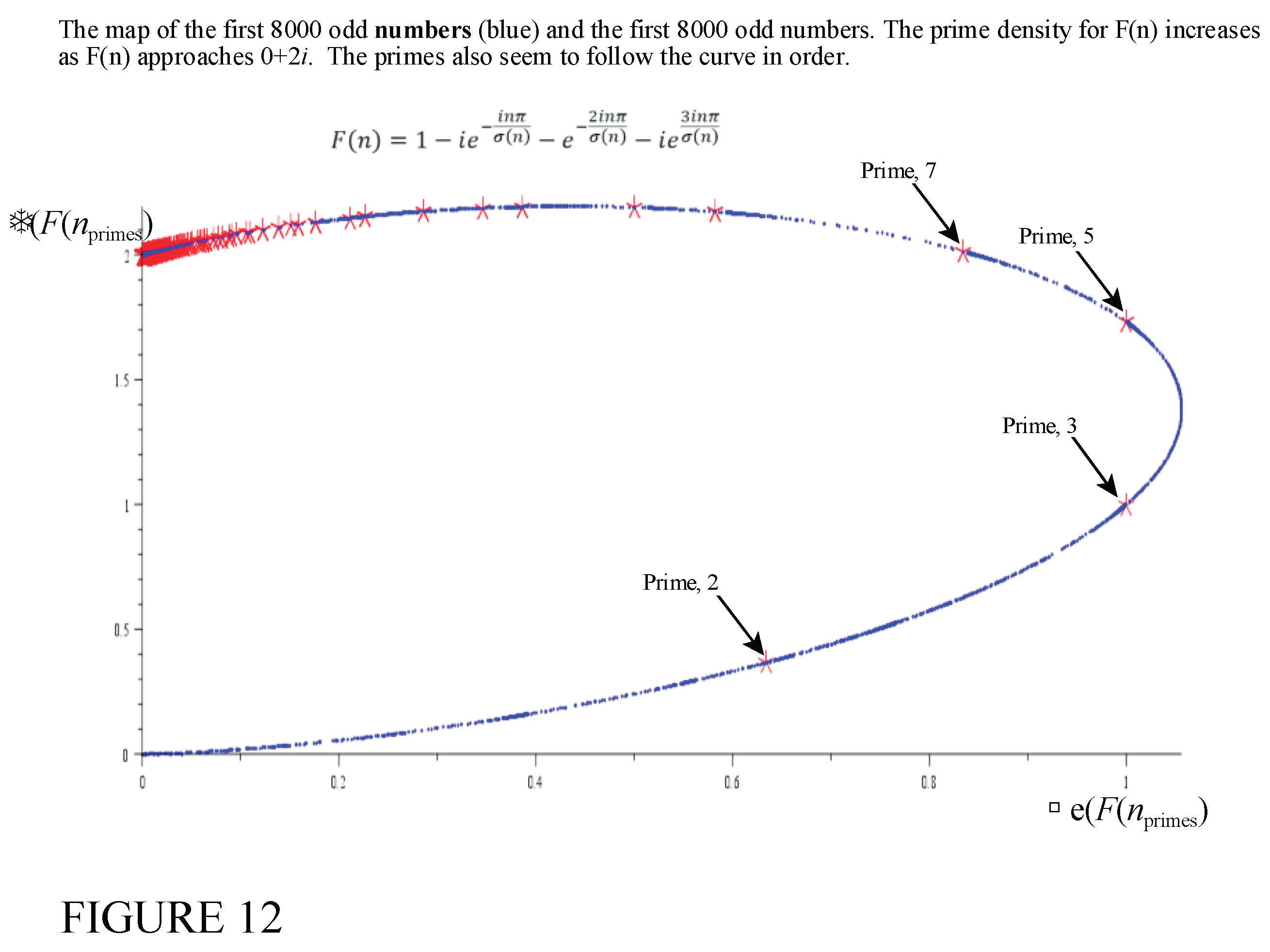
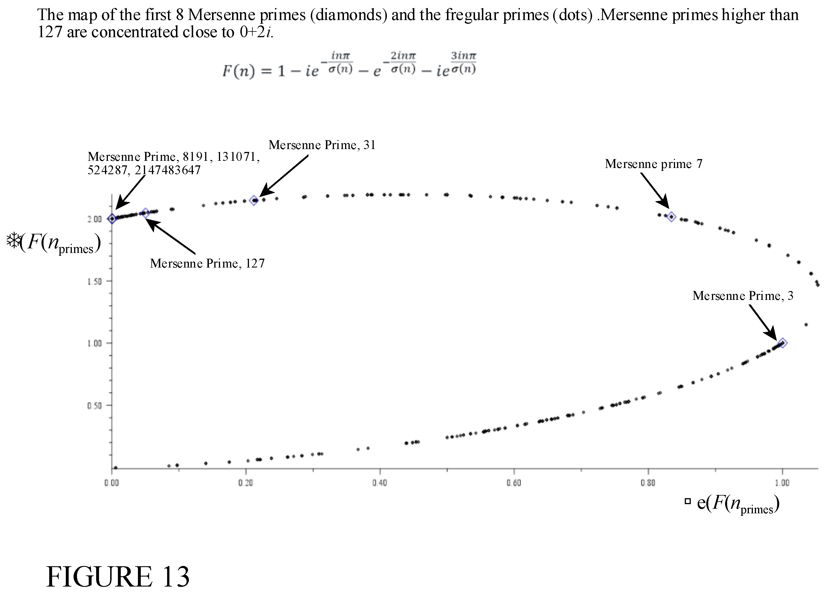
Figure 13 shows the distribution of the Mersenne primes with the regular primes.

6. The Extension of TH Function F(n) to a General Series Form

The function

$$F\left(n\right)=1-i{e}^{-{\displaystyle \frac{in\pi }{\sigma \left(n\right)}}}-e^{-{\displaystyle \frac{2in\pi }{\sigma \left(n\right)}}}-i{e}^{{\displaystyle \frac{3in\pi }{\sigma \left(n\right)}}}$$

(40)

behaves like a CyclotomicPolynomial. CyclotomicPolynomialare the minimal polynomials of primitive roots of unity with rational coefficients. The first few CyclotomicPolynomial are shown below:

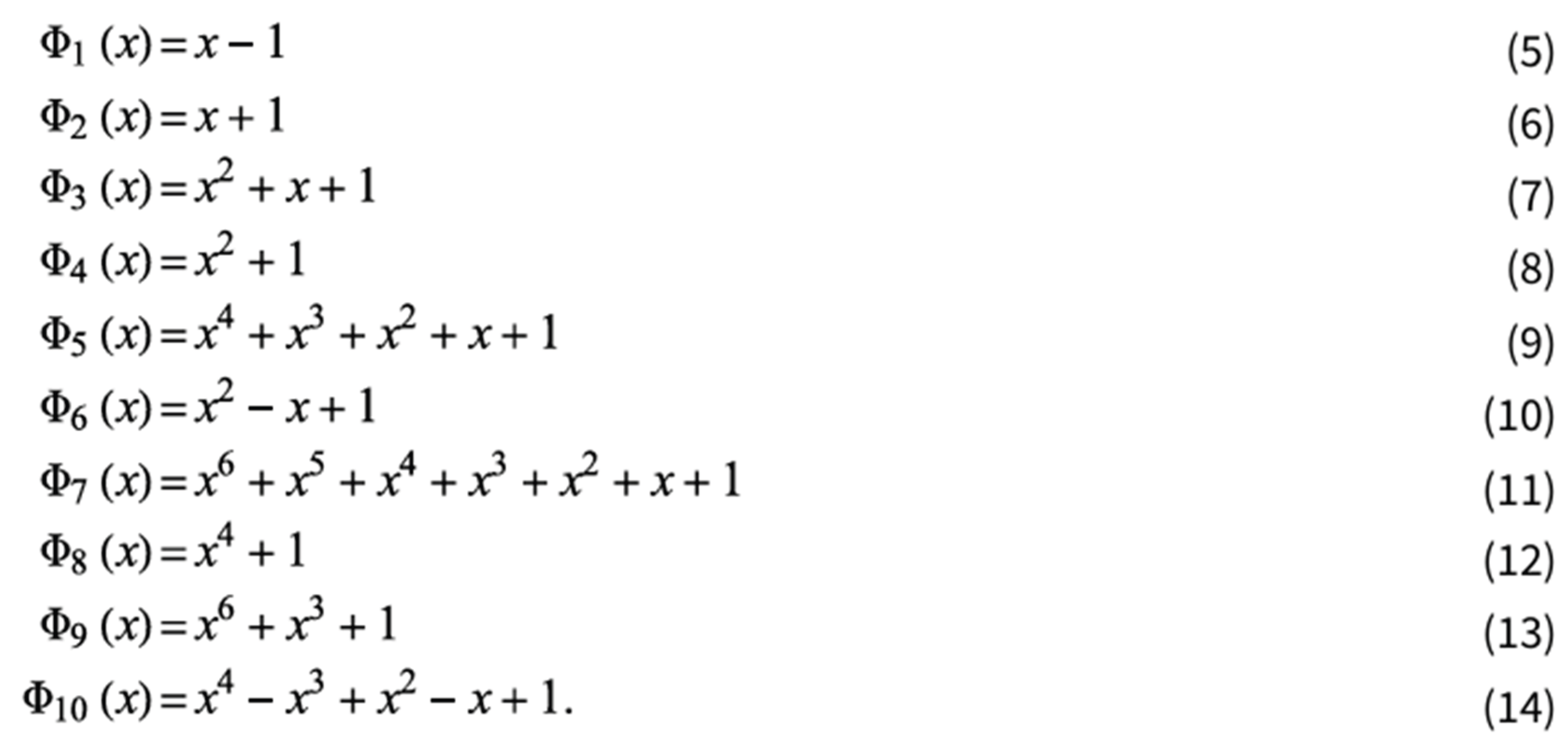
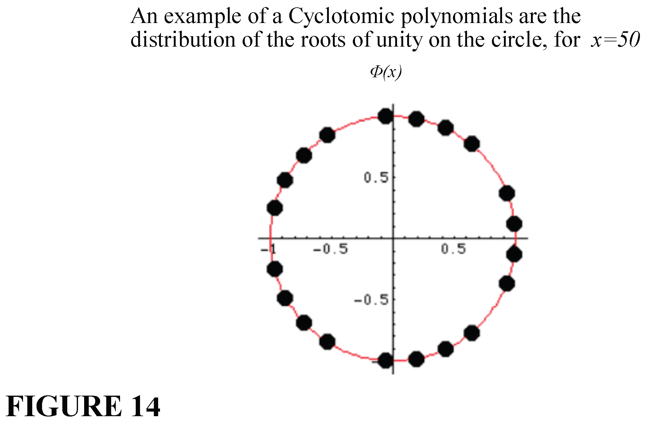
A cyclotomic polynomial is of the product form:

$${\mathsf{\Phi }}_m\left(x\right)=\prod _{k=1}^m\left(x-{\zeta }_m\right)$$

(41)

where, ${\zeta }_m$, are the roots of unity in the complex plane, $\mathbb{C}$ . In general, the circle, ${\zeta }_m=e^{\pi i\left(\omega \left(x\right)\right)} where \omega \left(x\right)={\displaystyle \frac{k}{m}},$and $k$ is taken over integers relative prime to $m.$ It is clear that the function

$$F\left(n\right)=1-i{e}^{-{\displaystyle \frac{in\pi }{\sigma \left(n\right)}}}-e^{-{\displaystyle \frac{2in\pi }{\sigma \left(n\right)}}}-i{e}^{{\displaystyle \frac{3in\pi }{\sigma \left(n\right)}}}$$

(42)

is composed of functions of cyclotomic polynomials for the the special case of an expansion of some function over the function ${\displaystyle \frac{n}{\sigma \left(n\right)}}.$Looking at exponential terms with the sequence, $0, -i, 2i, 3i,$we determine the first difference in the powers to be

$${\delta }_1 \to -i, 3i, i,$$

(43)

The second difference gives,

$${\delta }_2 \to 4i,-2i,$$

(44)

The second difference points to the function $F\left(n\right),$ following a sequence of powers that is purely linear, but quadratic or alternating in some manner. We assume a quadratic relation, of the form, $A{k}^2+Bk+C.$ However, the second differences are not the same constants, and so a recurrence relation of the form, $b_k=f\left(b_{k-1},b_{k-2} \right)$must be used to expand $F\left(n,m\right)$ as a series of higher powers for $m$ recurrenses. The sequence of powers in $F\left(n,m\right),$ follows the recurrence, with initial conditions,

$$b_k=-b_{k-1}-7b_{k-2}, { b}_0=0, b_2=-i$$

(45)

The characteristic equation for the recurrence then yeilds,

$$r^2+2r+7=0$$

(46)

This yields, the two solutions,

$$\begin{array}{c}{r}_1=-1-i\sqrt{6}\\ r_2=-1+i\sqrt{6}\end{array}$$

(47)

Since the recurrence (46) follows a second order linear form, the general solution of the recurrence is

$$b_k=C_1{r_1}^k+C_2{r_2}^k , C_1, C_2 are constants.$$

(48)

Solcing for$C_1,$ and $C_2,$we get:

$$C_1=-{\displaystyle \frac{\sqrt{6}}{84}}+{\displaystyle \frac{i}{14}} , C_2={\displaystyle \frac{\sqrt{6}}{84}}+{\displaystyle \frac{i}{14}}$$

(49)

Hence we get

$$b_k=\left(-{\displaystyle \frac{\sqrt{6}}{84}}+{\displaystyle \frac{i}{14}}\right){\left(-1-\sqrt{6}\right)}^k+\left({\displaystyle \frac{\sqrt{6}}{84}}+{\displaystyle \frac{i}{14}}\right){\left(-1+\sqrt{6}\right)}^k$$

(50)

Hence we have the general form for $m$ terms:

$$F\left(n,m\right)=\sum _{k=1}^m{\left({\displaystyle \frac{\left(-\frac{\sqrt{6}}{84}+\frac{i}{14}\right){\left(-1-\sqrt{6}\right)}^k +\left(\frac{\sqrt{6}}{84}+\frac{i}{14}\right){\left(-1+\sqrt{6}\right)}^k}{k-1}}\right)}^{k-1}{e}^{\left({\displaystyle \frac{\pi in}{\sigma \left(n\right)}}\right)\left(-{\displaystyle \frac{\sqrt{6}}{84}}+{\displaystyle \frac{i}{14}}\right){\left(-1-\sqrt{6}\right)}^k +\left({\displaystyle \frac{\sqrt{6}}{84}}+{\displaystyle \frac{i}{14}}\right){\left(-1+\sqrt{6}\right)}^k}$$

(51)

This sum produces the first four terms giving the same function:

$$F\left(n, 4\right)=1-i{e}^{-{\displaystyle \frac{in\pi }{\sigma \left(n\right)}}}-e^{-{\displaystyle \frac{2in\pi }{\sigma \left(n\right)}}}-i{e}^{{\displaystyle \frac{3in\pi }{\sigma \left(n\right)}}}$$

(52)

The function,

$$F\left(n,m\right)=\sum _{k=1}^m{\left({\displaystyle \frac{b_k}{k-1}}\right)}^{k-1}{e}^{\left({\displaystyle \frac{\pi in{b}_k}{\sigma \left(n\right)}}\right)}$$

(53)

will only have coefficients that are $\pm$1, or $-i$, for the first 4 terms, $m=4$. The remaining terms $m>4$ have large coefficients that blow up quickly. For example for m=7,

$$F\left(n, 7\right)=1-i{e}^{-{\displaystyle \frac{in\pi }{\sigma \left(n\right)}}}-e^{-{\displaystyle \frac{2in\pi }{\sigma \left(n\right)}}}-i{e}^{{\displaystyle \frac{3in\pi }{\sigma \left(n\right)}}} +625e^{-{\displaystyle \frac{20in\pi }{\sigma \left(n\right)}}}+{\displaystyle \frac{2476099}{3125}}{e}^{{\displaystyle \frac{19in\pi }{\sigma \left(n\right)}}}-24137569e^{{\displaystyle \frac{102in\pi }{\sigma \left(n\right)}}}$$

(54)

In general, for Perfect numbers,

$$\begin{gathered} F\left(n, 4\right)=1-i{e}^{-{\displaystyle \frac{in\pi }{\sigma \left(n\right)}}}-e^{-{\displaystyle \frac{2in\pi }{\sigma \left(n\right)}}}-i{e}^{{\displaystyle \frac{3in\pi }{\sigma \left(n\right)}}} =0, \\ F\left(n=5..\infty \right)=625e^{-{\displaystyle \frac{20in\pi }{\sigma \left(n\right)}}}+{\displaystyle \frac{2476099}{3125}}{e}^{{\displaystyle \frac{19in\pi }{\sigma \left(n\right)}}}-24137569e^{{\displaystyle \frac{102in\pi }{\sigma \left(n\right)}}}+\dots {\left({\displaystyle \frac{b_k}{k-1}}\right)}^{k-1}{e}^{\left({\displaystyle \frac{\pi in{b}_k}{\sigma \left(n\right)}}\right)} \end{gathered}$$

(55)

In general, we have:

$$F\left(n,\infty \right)= \sum _{k=1}^{\infty }{e}^{i\pi {\beta }_k} ,$$

(56)

Table 1. shows the functional relations of $F\left(n,\infty \right)= \sum _{k=1}^{\infty }{e}^{i\pi {\beta }_k}.$

$k$	${\beta }_k$
$1$	$0$
$2$	$-{\displaystyle \frac{1}{2}}-{\displaystyle \frac{n}{\sigma \left(n\right)}}$
$3$	$1+{\displaystyle \frac{2n}{\sigma \left(n\right)}}$
$4$	$-{\displaystyle \frac{1}{2}}+{\displaystyle \frac{3n}{\sigma \left(n\right)}}$
$5$	$-{\displaystyle \frac{20n}{\sigma \left(n\right)}}-{\displaystyle \frac{i\log 5^5}{\pi }}$
6	${\displaystyle \frac{1}{2}}+{\displaystyle \frac{19n}{\sigma \left(n\right)}}-i\left({\displaystyle \frac{\log {19}^5+\log 5^5}{\pi }}\right)$
7	$1+{\displaystyle \frac{102 n}{\sigma \left(n\right)}}-i{\displaystyle \frac{\log {17}^6}{\pi }}$
8	${\displaystyle \frac{1}{2}}-{\displaystyle \frac{337 n}{\sigma \left(n\right)}}-{\displaystyle \frac{i}{\pi }}\log {\left({\displaystyle \frac{337}{7}}\right)}^7$
9	$-{\displaystyle \frac{40 n}{\sigma \left(n\right)}}-{\displaystyle \frac{i}{\pi }}\log \left(5^8\right)$
10	${\displaystyle \frac{1}{2}}+{\displaystyle \frac{2439 n}{\sigma \left(n\right)}}-{\displaystyle \frac{i}{\pi }}\log {\left(271\right)}^9$

Table 1. shows the functional relations of $F\left(n,\infty \right)= \sum _{k=1}^{\infty }{e}^{i\pi {\beta }_k}.$

$k$	${\beta }_k$
$1$	$0$
$2$	$-{\displaystyle \frac{1}{2}}-{\displaystyle \frac{n}{\sigma \left(n\right)}}$
$3$	$1+{\displaystyle \frac{2n}{\sigma \left(n\right)}}$
$4$	$-{\displaystyle \frac{1}{2}}+{\displaystyle \frac{3n}{\sigma \left(n\right)}}$
$5$	$-{\displaystyle \frac{20n}{\sigma \left(n\right)}}-{\displaystyle \frac{i\log 5^5}{\pi }}$
6	${\displaystyle \frac{1}{2}}+{\displaystyle \frac{19n}{\sigma \left(n\right)}}-i\left({\displaystyle \frac{\log {19}^5+\log 5^5}{\pi }}\right)$
7	$1+{\displaystyle \frac{102 n}{\sigma \left(n\right)}}-i{\displaystyle \frac{\log {17}^6}{\pi }}$
8	${\displaystyle \frac{1}{2}}-{\displaystyle \frac{337 n}{\sigma \left(n\right)}}-{\displaystyle \frac{i}{\pi }}\log {\left({\displaystyle \frac{337}{7}}\right)}^7$
9	$-{\displaystyle \frac{40 n}{\sigma \left(n\right)}}-{\displaystyle \frac{i}{\pi }}\log \left(5^8\right)$
10	${\displaystyle \frac{1}{2}}+{\displaystyle \frac{2439 n}{\sigma \left(n\right)}}-{\displaystyle \frac{i}{\pi }}\log {\left(271\right)}^9$

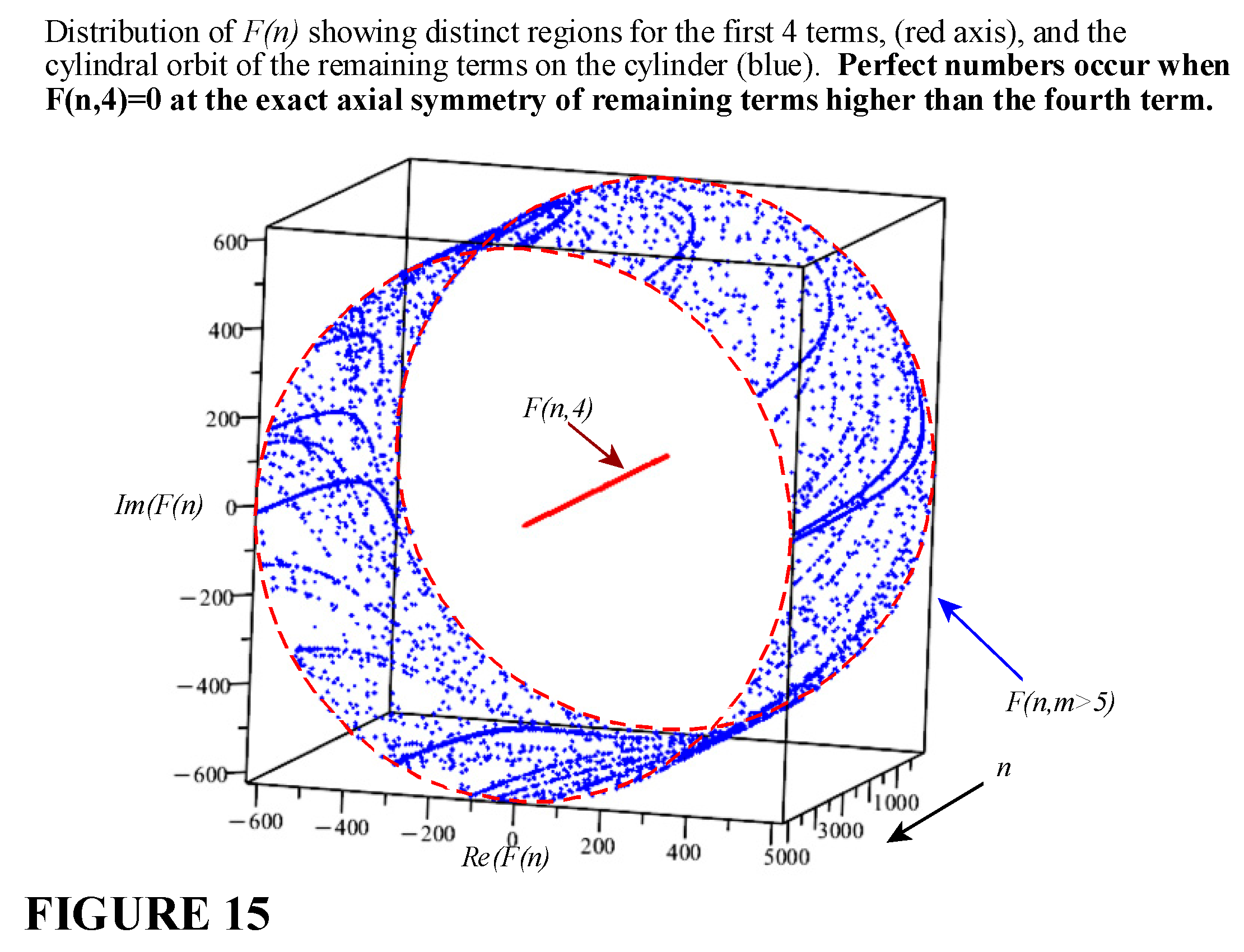
A 3-d plot of the function, shows that the function $F\left(n, 4\right)=0,$is the axis of an infinite cylinder ,where the rest of the terms $m>4$ lie.

Figure 15 shows the cylinderical form with the axis approaching a line when the cylinder radius approaches infinity. The axis of the cylinder becomes the solutions for Perfect numbers,

$$1-i{e}^{-{\displaystyle \frac{in\pi }{\sigma \left(n\right)}}}-e^{-{\displaystyle \frac{2in\pi }{\sigma \left(n\right)}}}-i{e}^{{\displaystyle \frac{3in\pi }{\sigma \left(n\right)}}}=0,$$

(57)

Hence for a Perfect number $N$, (57) gives:

$$N_p={\displaystyle \frac{\tan \left(2\right)\prod _{k=1}^{N_p}\left(1-\frac{{\sin }^2\left(\frac{1}{N_p}\right)}{{\sin }^2\left(\frac{\left(2k-1\right)\pi }{4N_p}\right)}\right)}{ \sin \left(\frac{2}{N_p}\right)\left(\prod _{k=1}^{N_p-1}\left(1-\frac{{\sin }^2\left(\frac{1}{N_p}\right)}{{\sin }^2\left(\frac{k\pi }{2N_p}\right)}\right)\right)}}$$

(58)

Theorem: (Prime Class Superposition):

For any subset of primes,$p\in \mathbb{P},$with$T\in \left(0,\pi \right)\subset \mathbb{R},A_k={\displaystyle \frac{2^{2k}\left|B_{2k}\right|}{\left(2k\right)!}} ,A_p={\displaystyle \frac{2^{2p}\left|B_{2p}\right|}{\left(2p\right)!}},$the cotangent -Bernoulli field satifies

$$\sum _{p\in \mathbb{P}}{A}_p{T}^{2p+1}\le \sum _{k\notin \mathbb{P}}{A}_k{\left(T\right)}^{2k+1} , 0<T<\pi$$

(59)

with and there are an infinite number of each such subset of primes,$\mathbb{P}$.

Proof:

Setup:

Let

$$\cot \left(x\right)={\displaystyle \frac{1}{2}}-\sum _{k=1}^{\infty }{\displaystyle \frac{2^{2k}\left|B_{2k}\right|}{\left(2k\right)!}}{x}^{2k-1} , \left[2^2<{\pi }^2\right]$$

(60)

Fix $x_0=T\in \left(0,\pi \right) with \cot \left(x_0\right)\in \mathbb{R}\backslash \left\{0\right\}.$Partition$\mathbb{N}$, into disjoint classes $\mathbb{P}$, and $\aleph =\mathbb{N}\backslash \mathbb{P},$where $\mathbb{P}$ is a class of primes, $p$.

Define

$$S_{all}\left(T\right)=\sum _{k\ge 1}^{\infty }{\displaystyle \frac{2^{2k}\left|B_{2k}\right|}{\left(2k\right)!}}{T}^{2k-1}, S_{\mathbb{P}}\left(T\right)=\sum _{p\in \mathbb{P}}^{\infty }{\displaystyle \frac{2^{2p}\left|B_{2p}\right|}{\left(2p\right)!}}{T}^{2p-1}, S_{\mathbb{N}}\left(T\right)=S_{all}-S_{\mathbb{P}}\left(T\right)$$

(61)

Note , $\left\{S_{all}\left(T\right),S_{\mathbb{N}}\left(T\right), S_{\mathbb{P}}\left(T\right)\right\}>0$for $T\in \left(0,\pi \right).$With the set up above, at a fixed $T\in \left(0,\pi \right),$ suppose the following holds true:

• (Regularity/positivity of coefficients)

Each summand is positive and satisfies the classical Bernoulli-Zeta representation:

$$\left|B_{2k}\right|={\displaystyle \frac{2\left(2k\right)!}{{\left(2\pi \right)}^{2k}}}\zeta \left(2k\right), k\in \mathbb{Z}$$

(62)

Hence, $S_{all}\left(T\right)\in \left(0, \infty \right).$

• b. (Analytic density at)

$T$

The decomposition of $\cot \left(T\right),\cot \left(2T\right)\mathrm{t}\mathrm{h}\mathrm{r}\mathrm{o}\mathrm{u}\mathrm{g}\mathrm{h} S_{N\left(x\right)}, S_{M\left(x\right)} y$ields a normalized cubic identity.

$$\cot \left(2T\right)={\displaystyle \frac{1}{2T}}-\sum _{k=1}^{\infty }{\displaystyle \frac{2^{2k}\left|B_{2k}\right|}{\left(2k\right)!}}{\left(2T\right)}^{2k-1} \left[{\left(2T\right)}^2<{\pi }^2\right]$$

(63)

$$\cot \left(2T\right)={\displaystyle \frac{1}{2T}}-\sum _{k=1}^{\infty }{\displaystyle \frac{2^{4k-1}\left|B_{2k}\right|}{\left(2k\right)!}}{\left(T\right)}^{2k-1} \left[{\left(2T\right)}^2<{\pi }^2\right]$$

(64)

From the cotangent relation, we have,

$$\cot \left(2T\right)={\displaystyle \frac{1}{2T}}-\sum _{k=1}^{\infty }{\displaystyle \frac{2^{k-1}\left(2^k-1\right)\left|B_{2k}\right|2^{3k}}{\left(2^k-1\right)\left(2k\right)!}}{T}^{2k-1} \left[{\left(2T\right)}^2<{\pi }^2\right]$$

(65)

This is an example of the decomposition of the cotangent to Perfect number as an example. Since a perfect number for $p$ a prime is given by, $N_p=2^{p-1}\left(2^p-1\right)$, (65) where $P_M=2^p-1$ is a Merseene prime, we can up for Mersenne primes, with $N_p=2^{p-1}\left(P_M\right)$

$$\cot \left(2T\right)={\displaystyle \frac{1}{2T}}-\sum _{p\in \mathbb{P}}{\displaystyle \frac{N_p\left|B_{2p}\right|2^{3p}}{P_M\left(2p\right)!}}{T}^{2p-1}+\sum _{k\notin \mathbb{P}}{\displaystyle \frac{2^{4k-1}\left|B_{2k}\right|}{\left(2k\right)!}}{\left(T\right)}^{2k-1} \left[{\left(2T\right)}^2<{\pi }^2\right]$$

(66)

Put, $A_p={\displaystyle \frac{N_p\left|B_{2p}\right|2^{3p-1}}{P_M\left(2p\right)!}}={\displaystyle \frac{\left|B_{pk}\right|2^{4p-1}}{\left(2p\right)!}},A_k= {\displaystyle \frac{\left|B_{2k}\right|2^{4k-1}}{\left(2k\right)!}}$ and multiply by $T$,

$$\cot \left(2T\right)={\displaystyle \frac{1}{2T}}-\sum _{p\in \mathbb{P}}{A}_p{T}^{2p}+\sum _{k\notin \mathbb{P}}{A}_k{\left(T\right)}^{2k} \left[{\left(2T\right)}^2<{\pi }^2\right]$$

(67)

Multiply across by $T$,

$$T\cot \left(2T\right)={\displaystyle \frac{1}{2}}-\sum _{p\in \mathbb{P}}{A}_p{T}^{2p}-\sum _{k\notin \mathbb{P}}{A}_k{\left(T\right)}^{2k} \left[{\left(2T\right)}^2<{\pi }^2\right]$$

(68)

Again multiply by $T again,$

$$T^2\cot \left(2T\right)={\displaystyle \frac{T}{2}}-\sum _{p\in \mathbb{P}}{A}_p{T}^{2p+1}-\sum _{k\notin \mathbb{P}}{A}_k{\left(T\right)}^{2k+1}$$

(69)

Again multiply by $T$,

$$\begin{gathered} T^3\cot \left(2T\right)={\displaystyle \frac{1}{2}}{T}^2-\sum _{p\in \mathbb{P}}{A}_p{T}^{2p+1}-\sum _{k\notin \mathbb{P}}{A}_k{\left(T\right)}^{2k+1} \\ \cot \left(T\right)={\displaystyle \frac{1}{T}}-\sum _{k\ge 1}{C}_k{\left(T\right)}^{2k-1}, C_k={\displaystyle \frac{2^{2k}\left|B_{2k}\right|}{\left(2k\right)!}} \end{gathered}$$

(70)

Note that $A_k= 2^{2k-1}{C}_k$;then,

$$T^3\cot \left(2T\right)-{\displaystyle \frac{1}{2}}{T}^2+{\displaystyle \frac{1}{4}}\cot \left(T\right)={\displaystyle \frac{1}{4}}\sum _{k\ge 1}{A}_k{\left(T\right)}^{2k+2}$$

(71)

Spilliting the RHS for primes and non-primes,

$$T^3\cot \left(2T\right)-{\displaystyle \frac{1}{2}}{T}^2+{\displaystyle \frac{1}{4}}\cot \left(T\right)={\displaystyle \frac{1}{4}}\left(\sum _{p\in \mathbb{P}}{A}_p{T}^{2p+1}-\sum _{k\notin \mathbb{P}}{A}_k{\left(T\right)}^{2k+1}\right)$$

(72)

$$T^3\cot \left(2T\right)-{\displaystyle \frac{1}{2}}{T}^2+{\displaystyle \frac{1}{4}}\cot \left(T\right)-{\displaystyle \frac{1}{4}}\sum _{k\notin \mathbb{P}}{A}_k{\left(T\right)}^{2k+1} = {\displaystyle \frac{1}{4}}\sum _{p\in \mathbb{P}}{A}_p{T}^{2p+1}$$

(73)

$$A_p={\displaystyle \frac{N_p\left|B_{2p}\right|2^{3p-1}}{P_M\left(2p\right)!}}$$

(74)

$$T^3\cot \left(2T\right)-{\displaystyle \frac{1}{2}}{T}^2+{\displaystyle \frac{1}{4}}\cot \left(T\right)-{\displaystyle \frac{1}{4}}\sum _{k\notin \mathbb{P}}{A}_p{\left(T\right)}^{2k+1} = {\displaystyle \frac{1}{4}}\sum _{p\in \mathbb{P}}{A}_k{T}^{2p+1}$$

(75)

$$\sum _{p\in \mathbb{P}}{A}_p{T}^{2p+1}>0 , \left(0<T<{\displaystyle \frac{\pi }{2}}\right)$$

(76)

Hence,

$$T^3\cot \left(2T\right)-{\displaystyle \frac{1}{2}}{T}^2+{\displaystyle \frac{1}{4}}\cot \left(T\right)>{\displaystyle \frac{1}{4}}\sum _{k\notin \mathbb{P}}{A}_k{\left(T\right)}^{2k+1}$$

(77)

Using, $B_{2k}~{\displaystyle \frac{2\left(2k\right)!}{{\left(2\pi \right)}^{2k}}}$, we have, $A_p~{\displaystyle \frac{4}{{\pi }^2}} ,$ and so the prime sum converges absolutely for $\left|T\right|<{\displaystyle \frac{\pi }{2}} .$This also gives the easy bounds:

$$0<\sum _{p\in \mathbb{P}}{A}_p{T}^{2p+1}\le \left(\sum _{k\ge 2}{\left({\displaystyle \frac{4T^2}{{\pi }^2}}\right)}^{k}T=T·{\displaystyle \frac{{\left(\frac{4T^2}{{\pi }^2}\right)}^2}{1-{\left(\frac{4T^2}{{\pi }^2}\right)}^k}}\right), \left|T\right|<{\displaystyle \frac{\pi }{2}}$$

(78)

Since every prime is positive for $T>0,$

$$\sum _{p\in \mathbb{P}}{A}_p{T}^{2p+1}\le \sum _{k\notin \mathbb{P}}{A}_k{\left(T\right)}^{2k+1} , 0<T<\pi$$

(79)

Since $p\in \mathbb{P}$ can be any selection $\mathbb{P}$ of a class of primes, and the structure of (79) requires an infinitude of for both partitions, then there exists an infinitude of such primes, and, picking the infinitude of just primes, we can say that the sum expresses the infinitude of all prime class of any type including $p\in \left\{Twin Primes, Mersenne Primes, Sophie primes and so on\right\}$.

Universality across prime classes:

The right hand side is a linear projection of the full Bernoulli field onto any prime class. Equation (79) represents an analytic equilibrium between a sparse harmonic lattice (the Special prime classes such as Mersenne class indices) and the complementary dense continuum (non-prime class integers). The finiteness of either subset would destroy the analytic balance and invert the sign of cot(2T) and cot(T). Thus, the very existence of an infinite sum for all k, enforces the infinitude of both all classes of primes-a remarkable intersection of trigonometric analysis and arithmetic structure.

Scholze–Type Interpretation: The Analytic Perfectoid Field of Primes.

In the sense of Peter Scholze’s condensed and perfectoid mathematics, the cotangent–Bernoulli field defined by

$$T^3\cot \left(2T\right)-{\displaystyle \frac{1}{2}}{T}^2+{\displaystyle \frac{1}{4}}\cot \left(T\right)-{\displaystyle \frac{1}{4}}\sum _{k\notin \mathbb{P}}{A}_p{\left(T\right)}^{2k+1}= {\displaystyle \frac{1}{4}}\sum _{p\in \mathbb{P}}{A}_k{T}^{2p+1}$$

(80)

can be regarded as an analytic perfectoid object: a field whose infinitude is expressed through structural completeness rather than unbounded enumeration. Just as Scholze’s perfectoid spaces encode infinitely many p-power roots within a single topologically complete object, the above field condenses infinitely many prime interactions into a single analytic continuum. Each prime subset $\mathbb{P}\mathbb{\text{'}}\subseteq \mathbb{P}$ defines a restriction functor of this field, preserving analytic convergence and equality. Hence the total field is stable under all infinite prime-indexed limits-the exact hallmark of a perfectoid or condensed structure. In Scholze’s sense, infinity here is not a countable sequence of primes but the completion of all prime classes under the cotangent–Bernoulli transformation. Every finite truncation breaks equality, yet the full infinite limit remains invariant, demonstrating condensed completeness. Therefore, the Prime Class Superposition Theorem defines an analytic space that behaves as a real-domain analogue of a perfectoid field: an object infinitely generated but topologically closed, where prime subsets act as coherent morphisms rather than discrete elements. This provides a natural, modern interpretation of the theorem, placing it within the same conceptual lineage as Scholze’s perfectoid and condensed frameworks.

Remarks and Positioning

a)

Novelty.

The Theorem is not a re-statement of any single classical result; it’s a fusion: positivity + analytic identity apse ⇒ infinitude of each class. The closest analogues are Pringsheim (positivity constraints), Fabry/Hadamard (sparsity ↔ analytic behavior), and Tauberian methods (analytic facts ⇒ density/infinitude).

b. The normalization that produces a cubic in T encapsulates the single-valuedness of the trigonometric function at $x_0$; the vanishing discriminant is precisely the statement that the two algebraic branches coincide with the analytic branch. For finite partitions, that coincidence cannot match the true sign/phase unless both classes are infinite.

Robustness. The argument isn’t tied to $x_0=2$; any $x_0\in \left(0,\pi \right)$ with $\mathrm{c}\mathrm{o}\mathrm{t}\left(x_0\right)\ne 0,$yields the same conclusion under (H1), (H2) and (H3).

References

- Leonhard Euler; “Institutiones calculi differentialis cum eius usu in analysi finitorum ac doctrina serierum, volume 1”.
- C.F. Gauss; “Theoria residuorum biquadraticorum, Commentatio secunda;” Königlichen Gesellschaft der Wis-senschaften zu Göttingen, 1863, 95 - 148.
- Gradshteyn, I.S.; Ryzhik, I.M. Table of Integrals, Series, and Products, 7th ed.; Zwillinger, D., Jeffrey, A., Eds.; Academic Press: Cambridge, MA, USA, 2007. [Google Scholar] [CrossRef]
- Hamou, P. “Marin Mersenne”; Stanford Encyclopedia of Philosophy, May 2018.
- Mersenne Prime; Wolfram V2, (March 2023 Version 2, wolframcloud.com).
- The On-Line Encyclopedia of Integer Sequences; (OEIS A000668), (OEIS A000043).
- On the Density of the Abundant Numbers, Paul Erdös, Journal of the London Mathematical Society: Volumes,1-9, Issue 4, Pages: 241-320, October 1934.
- Michael, M. Anthony; Consequences of Invariant Functions for the Riemann Hypothesis (Advances in Pure Mathematics, 2025, 15(1), 36-72 ).
Disclaimer/Publisher’s Note: The statements, opinions and data contained in all publications are solely those of the individual author(s) and contributor(s) and not of MDPI and/or the editor(s). MDPI and/or the editor(s) disclaim responsibility for any injury to people or property resulting from any ideas, methods, instructions or products referred to in the content. |
© 2025 by the authors. Licensee MDPI, Basel, Switzerland. This article is an open access article distributed under the terms and conditions of the Creative Commons Attribution (CC BY) license (http://creativecommons.org/licenses/by/4.0/).
Copyright: This open access article is published under a Creative Commons CC BY 4.0 license, which permit the free download, distribution, and reuse, provided that the author and preprint are cited in any reuse.