
Submitted:
15 October 2025
Posted:
16 October 2025
You are already at the latest version
Abstract
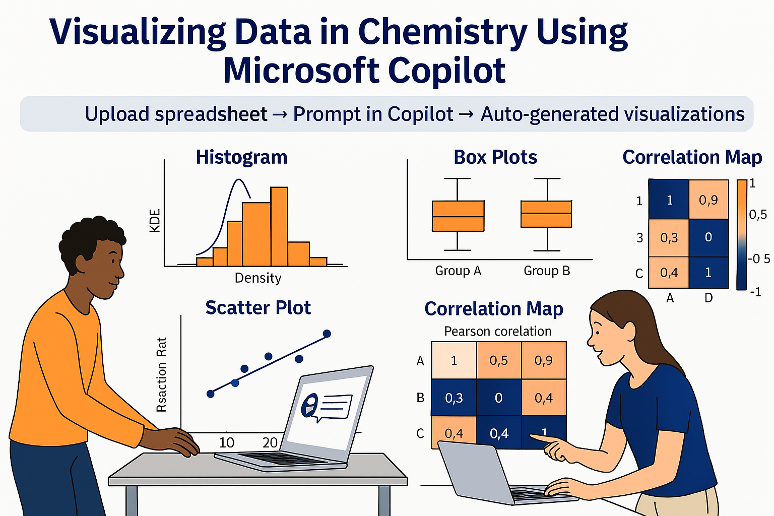
Large language models (LLMs) are increasingly integrated into education, yet their ability to perform calculation-based tasks and generate scientific visualizations has been limited. This study evaluates Microsoft Copilot (GPT 5) for chemistry education across four domains: (1) chemical equilibrium, pH, titration, and buffer calculations; (2) data visualization using histograms, box plots, correlation plots, and heatmaps; (3) multivariate analysis of periodic table properties through principal component analy-sis (PCA); and (4) image interpretation and creation in classroom contexts. Thir-ty-three representative questions were tested without additional prompting. Copilot delivered accurate, step-by-step solutions for acid–base and equilibrium problems, generated high-quality visualizations directly from uploaded datasets, and produced PCA score and loading plots with proper data standardization. These results indicate that GPT 5 significantly improves over earlier LLM versions, offering a practical tool for enhancing conceptual understanding and data literacy in chemistry education. However, limitations persist in interpreting complex chemical imagery, requiring hu-man oversight. Future work should focus on refining multimodal accuracy and devel-oping pedagogical frameworks for responsible AI integration.
Keywords:
copilot
; large language model
; artificial intelligence
; box plots
; calculations
1. Introduction
The advent of Large Language Models (LLMs) has marked a transformative era in artificial intelligence, particularly in their capacity to reshape digital interactions across healthcare, education, and economic sectors.[1]. Within educational contexts specifically, these AI systems have introduced paradigm-shifting capabilities in personalized instruction, adaptive tutoring, and dynamic content creation. Contemporary LLM implementations - including ChatGPT (OpenAI), Gemini (Google), Copilot (Microsoft), DeepSeek, and Perplexity - have achieved remarkable linguistic fluency, enabling natural language interactions accessible through common digital platforms. Their integration into learning ecosystems offers significant pedagogical advantages: facilitating immediate formative feedback, enhancing learner motivation, and providing intuitive access to complex problem-solving across STEM and humanities disciplines - all through conversational interfaces requiring no technical specialization.[2,3]
Since late 2023, ChatGPT has incorporated advanced multimodal capabilities, allowing it not only to generate text but also to analyze and produce images, upload spreadsheets and does complex calculations.[4,5] These features were introduced with the release of GPT-4 with Vision (GPT-4V), enabling users to upload and interpret visual content such as diagrams, graphs, tables, and handwritten notes. In parallel, the integration of the DALL·E model allows ChatGPT to generate images from text prompts and perform inpainting—editing specific regions of an image based on user input. These developments significantly expand the tool’s applicability in educational and research contexts, especially for tasks that require visual interpretation or the creation of illustrative content, such as conceptual diagrams, experimental setups, or visual summaries of data.[6,7]
As of May 2025, DeepSeek had reached its third iteration (V3), coinciding with the release of DeepSeek-R1—a low-cost yet powerful AI model that triggered a sharp downturn in the U.S. stock market.[8] The rapid ascent of DeepSeek has drawn global attention to China’s broader AI ecosystem, which functions under markedly different principles than those of Silicon Valley.[9]
R1 is part of a broader surge in Chinese LLMs development. Originating as a spin-off from a hedge fund, DeepSeek rose from relative obscurity with the release of its V3, which outperformed major competitors despite being developed on a modest budget.[10]
In 2024, Nascimento Júnior et al.[11] demonstrated that large language models (LLMs) can interpret and generate certain types of images. Alasadi & Baiz [12] demonstrated that ChatGPT (GPT-4) can successfully analyze images, including interpreting infrared (IR) spectra and molecular orbital diagrams of nitrogen.
In the healthcare domain, large language models (LLMs) such as ChatGPT, Gemini, and Copilot have contributed to improving prostate cancer literacy [13]. Several tools—including Bard, Bing, ChatGPT, Claude, and Gemini—have been employed in ophthalmology-related studies, particularly for multiple-choice examinations. These tools have been applied to answer patient inquiries, provide medical advice, support patient education, assist in triage, facilitate diagnosis and differential diagnosis, and contribute to surgical planning [14]. In eye care, ChatGPT has enhanced access to critical information, improved patient engagement, and streamlined triage processes [15]. Additionally, Copilot, Gemini, and ChatGPT-4 have been utilized for the interpretation of Western blot results [16]. Claude, Copilot, Gemini, ChatGPT, and Perplexity have also been employed to support postgraduate students in successfully passing the Specialty Certificate Examination in Dermatology [17].
In chemistry education, LLMs offer a compelling yet underexplored opportunity. Chemistry is inherently multimodal: learning often depends on interpreting symbolic, visual, and spatial information. Students are expected to construct and decode molecular structures, Lewis diagrams, orbital representations, and reaction mechanisms—skills that require both conceptual understanding and visual literacy.[18,19,20,21,22] While LLMs excel in linguistic tasks and factual recall, their ability to process or generate chemical imagery accurately remains a significant limitation.[11,12]
Recent studies suggest that although LLMs can describe chemical principles correctly, they frequently struggle with visual conventions and structural accuracy. For example, when prompted to generate Lewis structures or stereoisomeric diagrams, models often produce distorted or chemically invalid results.[23,24] This discrepancy raises concerns about the pedagogical reliability of these tools, particularly in introductory courses where students rely heavily on accurate visual aids to develop foundational understanding.[25]
Chatbots such as ChatGPT have been widely used in chemical education for tasks including scientific writing assignments,[26] enhancing critical thinking skills [27], answering chemistry questions [28,29,30], and writing lab reports. While chatbots can now upload datasets and generate images, their ability to create visualizations—such as box plots, histograms, principal component analysis plots, and supervised classification models—has not yet been described in the literature. This is a recent development, as only recently have chatbots gained the capability to handle data and produce graphical outputs. [5].
At the same time, the integration of image input and interpretation capabilities in modern LLMs introduces promising pathways for chemistry education. Multimodal models—capable of processing both text and images—can now identify functional groups in chemical diagrams, recognize reaction types from schemes, and classify molecular properties from image prompts .[31,32] These features may be particularly useful in visual tasks such as distinguishing between polar and nonpolar molecules, understanding the significance of conjugated systems in natural dyes, or interpreting organic transformations like reduction and hydrolysis. Such affordances point to a future where AI could serve as a conceptual scaffold, enabling students to explore chemical ideas interactively, even if the model lacks perfect visual precision.[33,34]
This study evaluates the capabilities and limitations of Copilot (GPT-5) in supporting chemistry education across diverse representational formats. Specifically, we examine its ability to: (1) perform calculations related to chemical equilibrium, pH, and titrations; (2) generate visualizations such as histograms, box plots, and correlation plots; (3) analyze physicochemical properties of periodic table elements through box plots, Pearson correlation heatmaps, principal component analysis (PCA), and correlation matrices; and (4) interpret and create images within classroom learning contexts. Our approach employs iterative prompting and performance benchmarking using tasks commonly encountered in high school and undergraduate chemistry curricula.
Overall, the findings provide a nuanced perspective on Copilot’s current role in chemistry education. Results support its cautious integration as a supplementary tool for conceptual reinforcement and chemical reasoning. Future advancements in multimodal training and domain-specific fine-tuning will be essential to fully realize the educational potential of these AI systems
2. Materials and Methods
3. Chemical Equilibrium
3.1. Chemical Equilibrium, Where K > 1
Although previous studies reported that, as of 2023, large language models (LLMs) often struggled with calculation-based questions [37,38]. Q1 presented an equilibrium problem involving an esterification reaction (Eq. 1), where the equilibrium constant . To address this, Copilot constructed an ICE (Initial, Change, Equilibrium) table (Table 2), substituted the equilibrium concentrations into the expression, and applied Bashara’s method to solve for . It then resolved the quadratic equation, identified the two mathematical solutions, and determined the only physically meaningful value. The detailed procedure is provided in the Supporting Information.
CH3COOH (ethanoic acid)+C2H5OH (ethanol) ⇌ CH3COOC2H5 +H2O
3.2. Strong Acid and Strong Base pH Calculation
In 2023, Clark et al. ³¹ reported that ChatGPT struggled with answering questions related to acid–base equilibrium (Table 1; Q2–Q11). Those question were responded using Copilot GPT-5. In Question 2 , it correctly identified HI as a strong acid, noted that its concentration equals the [H+] concentration, and calculated the pH using eq. 2.
In Q3, it recognized Sr(OH)₂ as a strong dibasic base, correctly applying [OH−]= 2[Sr(OH)2], and then determined the pOH using eq.3, followed by pH calculation using pH=14−pOH.
3.3. Weak Acid and Weak Base pH Calculation
In Q4 and Q5, it identified HF as a weak acid and CH₃NH₂ as a weak base, respectively. For the acid version, they constructed ICE tables and, given the small Ka value, applied the approximation shown in eq. 4, where Ka is equilibrium constant and F was the weak acid concentration. Then, it calculated the pH doing pH = -log10[H+]
For Q5, a similar approach was used: it set up ICE tables, approximated the [OH-] concentration as shown in eq. 5, calculated the pH, and converted pOH to pH. In both cases, chatbots calculated the degree of ionization afterward to confirm that the simplification F−x ≈ F was valid.
Copilot recognized the stoichiometry of the neutralization reaction, noting that 1 mole of H₂SO₄ reacts with 2 moles of KOH, and applied a direct stoichiometric calculation to determine the required volume of base. In the base version, they correctly identified that 2 moles of HCl react with 1 mole of Ca(OH)₂, performing the appropriate calculations to determine the amount of acid needed. In Q6, chatbots correctly recognized that both titrations were conducted beyond the equivalence point. In the acid version, they attributed the final pH to the excess strong acid; in the base version, the pH was determined based on the excess strong base. While Clark et al. [35] reported in 2023 that ChatGPT employed unusual reasoning strategies to solve acid–base problems (Questions 2–6), by June 2025, all evaluated chatbots demonstrated a conventional, step-by-step approach. These tools are now capable of delivering accurate and methodologically sound solutions to a wide range of acid–base equilibrium and neutralization problems, including those involving approximations, stoichiometry, and titration logic.
3.4. Salts pH Calculation
In Q6 and Q7, the chatbots correctly classified NH₄Cl as a weakly acidic salt and NaF as a weakly basic salt, respectively. Solving both problems using the same ICE table approach. The pH of the NH4Cl was calculated as the pH of a weak acid, and the pH of NaF was calculated as pH of weak base.
3.5. Neutralization
In Q8, it recognized the stoichiometry of the neutralization reaction, noting that 1 mole of H₂SO₄ reacts with 2 moles of KOH, and applied a direct stoichiometric calculation to determine the required volume of base. In Q9, it identified that 2 moles of HCl react with 1 mole of Ca(OH)₂, performing the appropriate calculations to determine the amount of acid needed.
3.6. Titration
In Q10, chatbots correctly recognized that both titrations were conducted beyond the equivalence point, attributed the final acid pH to the excess strong acid added to the weak base. In Q11, the pH was determined based on the excess strong base. While Clark et al. [35] reported in 2023 that ChatGPT employed unusual reasoning strategies to solve acid–base problems (Questions 2–6), by June 2025, Copilot demonstrated a conventional, step-by-step approach, delivering accurate and methodologically sound solutions to a wide range of acid–base equilibrium and neutralization problems, including those involving approximations, stoichiometry, and titration logic.
Q12-Q14 describes some titration questions that need calculations and some concepts such as differentiation between direct titrations and back titration.
Q12 is acid base titration involving the direct titration of ammonia in a household cleaner using sulfuric acid.[39] The cleaner was first diluted in a volumetric flask, and a measured portion of this solution was titrated. It successfully identified the stoichiometric relationship between ammonia and sulfuric acid, recognized that only a portion of the cleaner was used in the titration, and accurately calculated the percentage of ammonia in the cleaner.
Q13 is a direct redox titration involving the analysis of Mohr’s salt using KMnO₄.[40,41]. Copilot calculated the number of moles of Mohr’s salt based on the initial mass used in the titration. Using this information, they determined the number of water molecules in the salt’s hydration sphere.
Q14 concerns the back titration of aspirin [42,43,44]. Because aspirin is poorly soluble in water, a back-titration method was used. An excess of NaOH was added to neutralize the carboxylic acid group and hydrolyze the ester functionality. After heating, the remaining NaOH was titrated with a standard sulfuric acid solution. The mass of aspirin in the tablet was then determined based on the stoichiometric relationships between aspirin, NaOH, and H₂SO₄.
3.6. Buffer Calculation
Q15 addresses a buffer system [45,46], composed of a weak acid and its conjugate base. Copilot employed the Henderson–Hasselbalch equation to determine the amount of conjugate base needed to reach the target pH. This example illustrates that the model is capable of accurately performing buffer-related calculations
3.7. Calculation {H+] Ratio
Q16 involved the calculation of the pH of a strong acid (HCl) and a weak acid (acetic acid), followed by determining how many times the HCl solution has more [H⁺] ions than the acetic acid solution. All chatbots correctly calculated the pH of the HCl solution as 1, using the formula pH = -log₁₀[HCl], given that HCl is a strong acid and fully dissociates in solution.
They also correctly identified acetic acid as a weak acid. Since its Ka value is small, the pH was calculated using the approximation eq. 4. Furthermore, Copilot determined that the HCl solution contains approximately 75 times more H⁺ ions than the acetic acid solution. This result highlights their ability to perform chemical calculations and distinguish between strong and weak acids, demonstrating their potential as effective tools in chemistry education.
3.8. Building Titration Plots
During an acid–base titration, the pH of the solution varies progressively with the addition of titrant, showing a particularly sharp change near the equivalence point. Strong acids display a steeper and more pronounced pH transition at the equivalence point than weak acids, which exhibit a smoother curve due to buffering effects .[47,48]. In Q17, Copilot accurately described the pH behavior of both strong and weak acids during titration, clearly illustrating that strong acids undergo a sharper pH change near the equivalence point, whereas for weak acids, the pH at the half-equivalence point corresponds to the pKa (Figure 1).
4. Uploading Datasets and Building Images
This section was carried out using the dataset taken from Dong et al[49], the dataset is in the supporting information (Spreadsheet 1.xlsx). The study developed Parallel Reaction Monitoring (PRM) assays to quantify two urinary glycopeptides—FLN*ESYK from prostatic acid phosphatase (ACPP) and EDALN*ETR from clusterin (CLU)—as biomarkers for aggressive prostate cancer. Urine samples from 142 patients were analyzed, including 69 non-aggressive cases (Gleason score = 6) and 73 aggressive cases (Gleason score ≥ 8). The assays measured Light/Heavy ratios of these glycopeptides, normalized to heavy isotope-labeled standards, alongside clinical variables such as serum PSA and age.
4.1. Histograms
Histograms are a fundamental visualization tool for understanding how data points are distributed across different ranges (bins). By grouping observations into these bins, histograms reveal the overall shape of the data—whether it is skewed, uniform, or approximately normal—and help identify patterns such as clusters, gaps, or outliers. This makes them particularly useful in medical research for comparing characteristics between groups, such as benign and malignant tumors [50,51].
Kernel Density Estimation (KDE) curves, on the other hand, provide a smooth, continuous representation of the data distribution. Instead of discrete bars, KDE uses a mathematical function (the kernel) to estimate the probability density at each point, creating a curve that highlights where data points are concentrated. This approach is valuable for detecting subtle differences between groups and identifying multiple peaks or distribution shifts that might be hidden in a histogram.
When Spreadsheet 1 was uploaded and processed using the Q18 prompt, Copilot first generated separate histograms for ACPP_FLN*ESYK in NAG and AG patient groups (Figure 2). These plots revealed that the Light/Heavy ratios follow a skewed distribution, which becomes clearer when transformed to a logarithmic scale. Next, histograms were displayed using the log₁₀ transformation to reduce skewness and highlight relative differences between groups (Figure 3). Finally, Copilot produced an overlay plot (Figure 4) combining both groups on the same axis, showing that although aggressive and non-aggressive cases differ in central tendency, their concentration ranges partially overlap.
Q19 demonstrated Copilot’s ability to generate histograms on both linear and logarithmic scales. Initially, separate histograms for ACPP_FLN*ESYK in NAG and AG groups were created, revealing a highly skewed distribution. Applying a log transformation addressed this skewness by compressing extreme values, making the data more symmetric and easier to interpret. On the original scale, small changes at low concentrations appeared negligible compared to large values, whereas log scaling converted multiplicative differences into additive ones—so a two-fold increase looks the same whether from 0.1 to 0.2 or 10 to 20. Finally, overlaying both groups on a single plot allowed direct comparison, showing that while aggressive and non-aggressive cases differ in central tendency, their ranges partially overlap. This approach improves clarity and reduces the influence of outliers when visualizing biomarker distributions.
In Q19, Copilot generated histograms for both NAG and AG groups within the same plot. In the linear scale visualization (Figure 5), it was difficult to compare the groups due to the skewed distribution of the data. However, when the data was plotted using a logarithmic scale (Figure 6), the comparison between the two groups became much clearer and more interpretable.
In Q20, ages were normally distributed, so a linear scale was used (Figure 7), while PSA concentrations were shown on a log scale (Figure 8). Histograms indicate that aggressive tumors (AG) cluster at higher PSA values than non-aggressive tumors (NAG), and KDE curves highlight this trend with a sharp AG peak and a broader NAG distribution. For age, KDE curves show AG cases concentrated in older ranges, while NAG cases are more evenly spread. These patterns are key for understanding risk factors and guiding diagnosis.
4.2 Box Plots
Box plots are an important tool for visualizing data, particularly for comparing distributions and identifying outliers.[52,53]. Q21–Q25 focus on box plot visualizations. In Q21, Copilot generated box plots for ACPP_FLN*ESYK values on both a linear scale (Figure 9a) and a log-transformed scale (Figure 9b). The log transformation provided a clearer representation of the data distribution and highlighted group differences more effectively. Because the dataset did not satisfy normality assumptions, nonparametric tests were applied for group comparisons. The results from the box plots (Figure 9b), supported by Mann–Whitney tests, indicated that the AG group exhibited significantly higher ACPP_FLN*ESYK values compared to the NAG group.
In Q22, similar to Q21, Copilot generated box plots for CLU_EDALN*ETR values on both a linear scale (Figure 10a) and a log-transformed scale (Figure 10b). The log transformation enhanced the visualization of data distribution and group differences. Statistical analysis confirmed that the AG group had significantly higher CLU_EDALN*ETR values than the NAG group, as indicated by the box plots and supported by Mann–Whitney test results.
In Q23, Copilot generated box plots to compare age and serum PSA levels between groups. As shown in Figure 11a, the AG group was significantly older than the NAG group, as confirmed by the Mann–Whitney test. Figure 11b displays serum PSA values on a log10 scale, demonstrating that the AG group also presented significantly higher PSA levels compared to the NAG group.
4.3. Correlation Plots
Correlation plots were a good way to see if the variables were correlated, Q22-Q23 were about correlations between the data. In Q22, Copilot generated correlation plots for the NAG and AG groups (Figure 12). Although no significant correlation was observed between ACPP_FLN*ESYK and CLU_EDALN*ETR when considering the entire dataset, the relationship between these variables was comparatively stronger within the AG group than in the NAG group.
In Q23, the relationships between age and the biomarkers ACPP_FLN*ESYK and CLU_EDALN*ETR were analyzed separately for the AG and NAG groups (Figure 13). Correlation plots generated by Copilot revealed no significant association between age and either biomarker in both groups.
5. Exploring the Physicochemical Properties of Elements in the Periodic Table
Q24 -Q32use the dataset provided in Spreadsheet 2.xlsx (Supporting Information), which contains the physicochemical properties of the elements in the periodic table.[54] These questions involve working the physicochemical properties of elements in the periodic table.
5.1. Principal Component Analysis (PCA)
Unsupervised methods in machine learning are a class of algorithms that work with unlabeled data to identify hidden patterns and intrinsic structures. Unlike supervised methods, which require a labeled training dataset, unsupervised algorithms aim to discover relationships and organize data independently[55].
The ability of Copilot to perform unsupervised methods is particularly interesting in the classroom, as undergraduate and graduate chemometrics courses often struggle to provide graphical user interface (GUI) software for such applications.[56] While there are good free options available through coding platforms such as Python and R [57,58,59], many students are unfamiliar with programming, which can limit their accessibility.
Principal Component Analysis (PCA) is an unsupervised technique primarily used for dimensionality reduction. Its goal is to transform high-dimensional data into a smaller set of variables, called principal components, that capture the most significant variance in the original data [50,56,60,61,62,63,64]. By identifying the new axes along which the data varies the most, PCA allows for the visualization and simplification of complex datasets without losing crucial information [65].
PCA works by identifying the directions of maximum variance in the data. If the data is not normalized, features with a larger range of values (and thus, higher variance) will have a disproportionately strong influence on the principal components. This can lead to misleading results where the principal components are simply reflecting the scale of the original features rather than the underlying structure of the data. Standardization, a common form of normalization, ensures that all features are on the same scale, so that each feature's contribution is based on its actual importance and not its magnitude [65,66,67,68,69]. All chatbots correctly identified that the data required standardization prior to PCA analysis and automatically standardized the dataset before generating the score plots.
In Q25, Copilot generated the score plot, coloring the elements according to their respective groups (Figure 14). In Figure 14, Principal Component 1 (PC1) explains 43.8% of the total variance, while Principal Component 2 (PC2) accounts for 29.5%, together capturing approximately 73.3% of the overall variability in the dataset. These results demonstrate the effectiveness of Principal Component Analysis (PCA) in visualizing and summarizing the underlying structure of the data.
As shown in Figure 14, the transition metals are clustered in the center of the plot, halogens are positioned on the right side, alkali metals appear at the bottom, and the sixth-period transition metals are located at the upper left region of the plot.
In Q26, the loading plot was analyzed (Figure 15) to interpret the correlations among physicochemical properties and to relate them to the position of the elements in the score plot (Figure 14). In the loading plot, an angle of approximately 180° between variables indicates a negative correlation, a 90° angle represents no correlation, and a small angle reflects a strong positive correlation.
The plot shows a clear correlation among ionization energy, electron affinity, and electronegativity, while these variables are inversely related to atomic radius. It also indicates that boiling point, melting point, atomic mass, and density are closely related to each other but not correlated with ionization energy, electron affinity, or electronegativity.
By comparing the score plot (Figure 14) with the loading plot (Figure 15), it becomes evident that elements with high melting points, boiling points, atomic mass, and density are located in the upper left region of the score plot. In contrast, elements with high electronegativity, electron affinity, and ionization energy are positioned on the right side.
5.2. Correlation Plots of the Physicochemical Properties of Elements in the Periodic Table
In Q28, the correlations previously observed in the loading plot are also evident in the Pearson correlation heatmap (Figure 16). This heatmap illustrates the strength and direction of the relationships among the physicochemical properties of the elements in the periodic table.
In Q29–Q31, the relationships identified in the heatmap (Figure 16) were further explored. In Q29, the correlation between Boiling Point and Melting Point was examined (Figure 17). A strong overall correlation was observed; however, post-transition metals and carbon deviated noticeably from the correlation line.
In Q30, the relationship between Ionization Energy and Electron Affinity was analyzed (Figure 18). Although a general trend was apparent, hydrogen, carbon, oxygen, nitrogen, phosphorus, and the alkali metals deviated from the overall correlation.
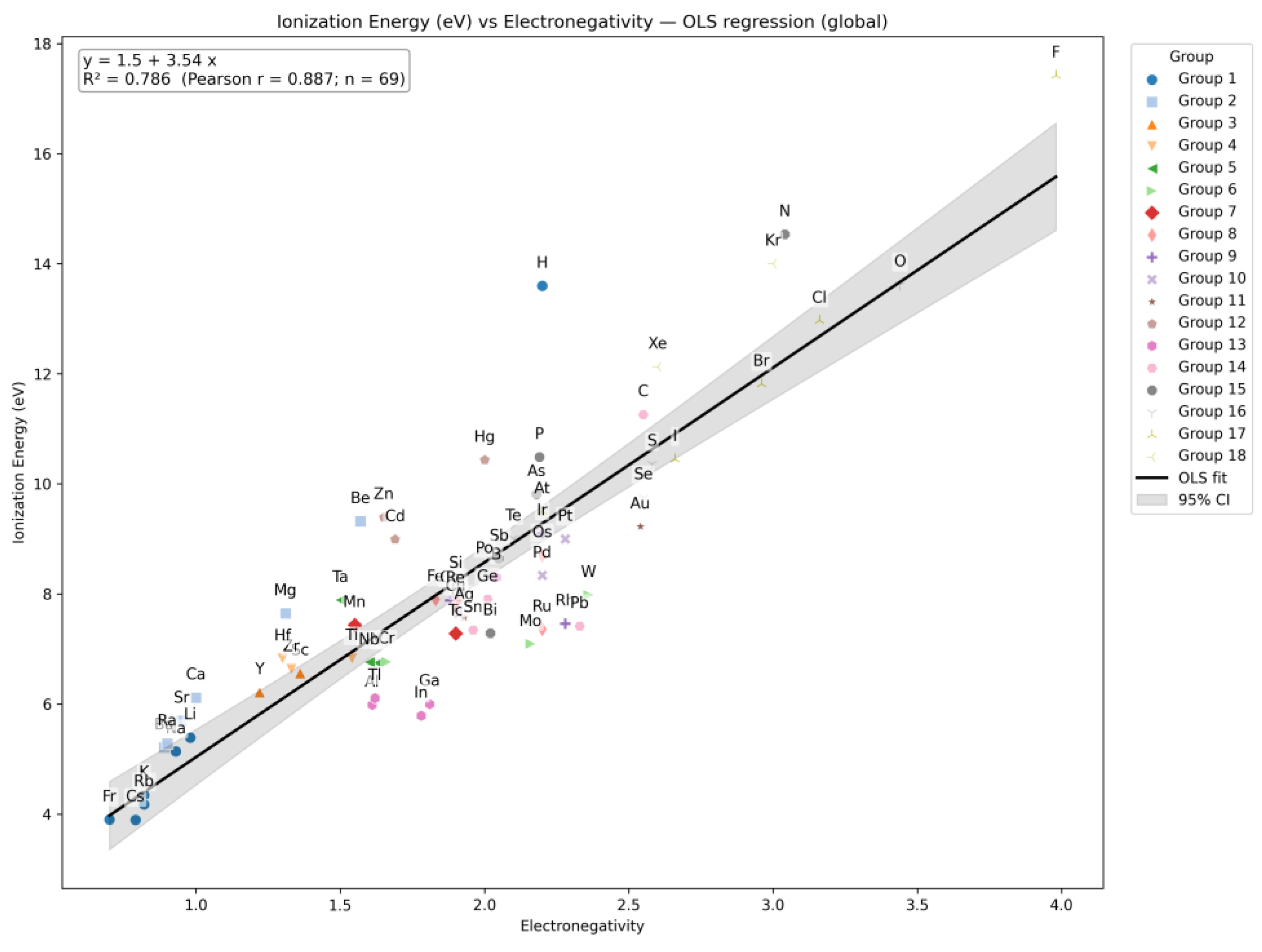
In Q31, the correlation between Ionization Energy and Electronegativity was examined. Questions Q27–Q30 collectively demonstrate a way to explore correlations among the physicochemical properties of chemical elements using correlation plots.
Figure 17.
Boiling Point vs. Melting Point.
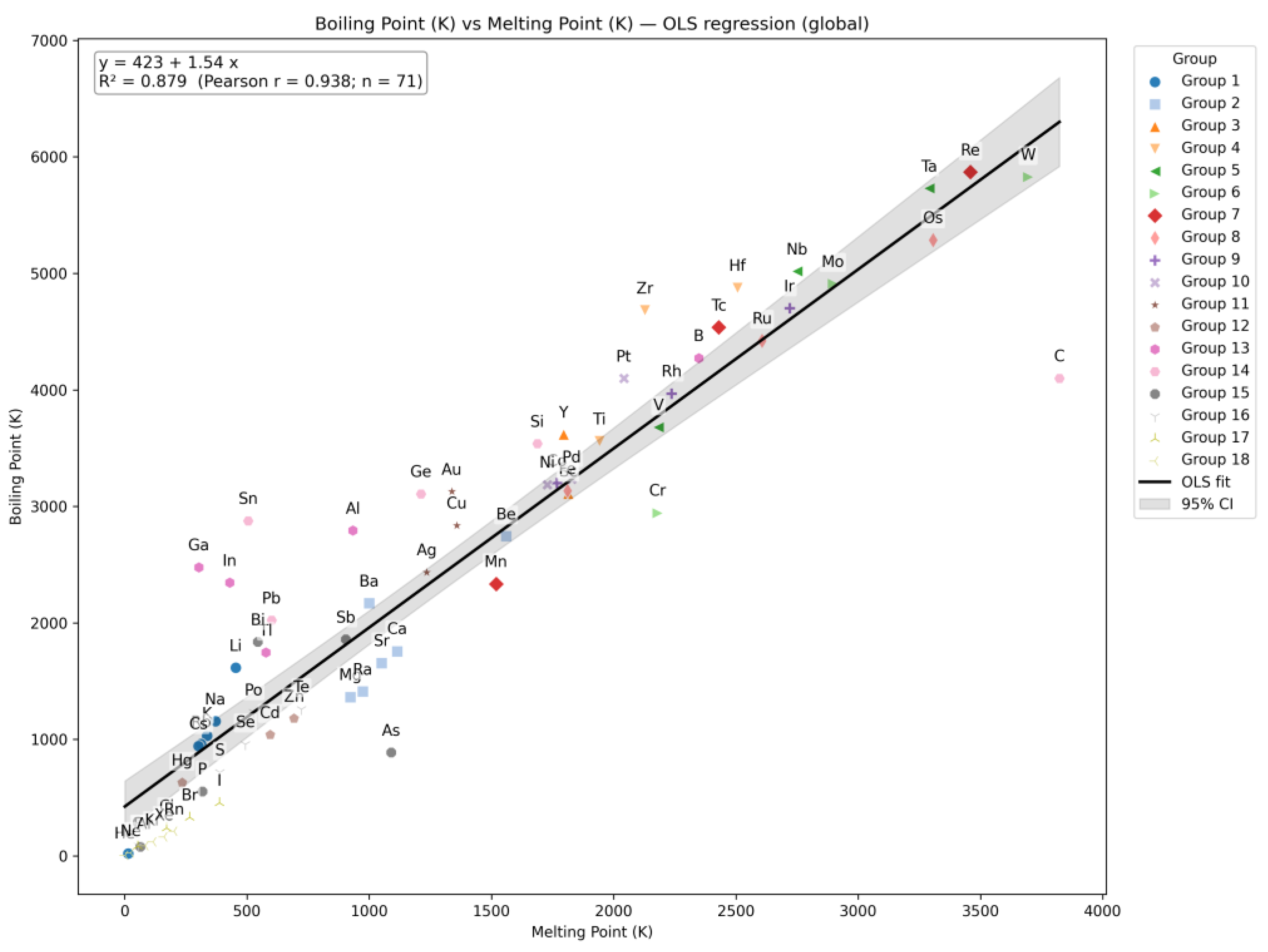
Figure 18.
Ionization Energy vs. Electron Affinity.
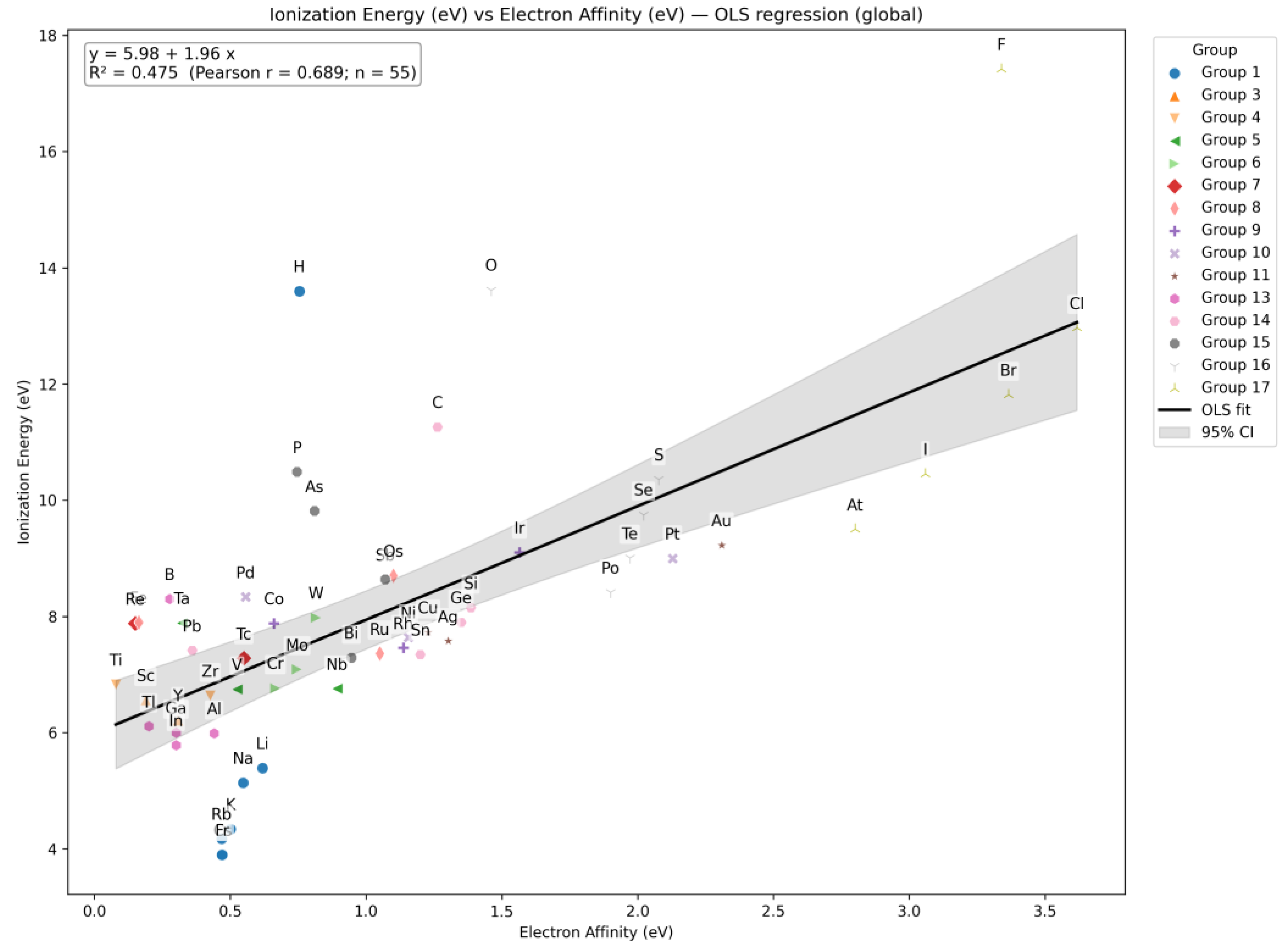
Figure 19.
Ionization Energy vs. Electronegativity.
In Q32, Copilot generated the box plots (Figure 20). Each plot illustrates the distribution and variability of physicochemical properties within each group, highlighting trends such as higher electronegativity and ionization energy in nonmetals, larger atomic radii and densities in metals, and intermediate values for metalloids. This question focuses on comparing physicochemical properties across different groups.
6. Image Interpretation and Generation in Classroom
Recently, chatbots can also upload and analyze images.[11,12]. To evaluate the ability of chatbots to interpret chemical reaction schemes, we selected a question involving a transesterification reaction. The chatbots were presented with the following prompt:
The analytical capabilities of chatbots—particularly their ability to process data and generate visual representations—can be effectively incorporated into laboratory instruction. For example, during a lab session, students measured the density of water using three types of glassware: a beaker (B), a volumetric pipette (V), and a graduated pipette (G). The objective was to illustrate that the beaker is unsuitable for precise volume measurements, whereas pipettes offer greater accuracy and reliability. This hands-on activity, supported by chatbot-assisted data visualization, reinforces key concepts in experimental design and measurement precision [70].
This objective was successfully achieved, as the results clearly showed that the pipettes provided more accurate and precise measurements than the beaker. Accuracy was assessed by how close the measured values were to the reference value (1.00 mg/mL), and precision was evaluated based on the interquartile range (IQR), with smaller IQR values indicating higher precision. The chatbot also identified an outlier in the graduated pipette group (0.6544 mg/mL), further enriching the analysis and discussion.
At the end of the class, students wrote their results on the chalkboard, and an image of the data was captured and uploaded to the Copilot application using a student's smartphone (Figure 21a). The prompt used was: "Build box plot for each group (beaker (B), volumetric pipette (V), and graduated pipette (G))." In response, Copilot generated the boxplots (Figure 21b) and provided a data-driven discussion. The boxplots clearly showed that the beaker yielded less precise results (larger IQR) compared to the pipettes, and that the pipettes were more accurate, as their median values were closer to the reference density (1.00 mg/mL).
Copilot enabled real-time data interpretation and visualization, improving learning outcomes. Each student was able to generate and analyze boxplots directly on their own smartphone, promoting engagement and deeper understanding of the concepts discussed.
Conclusion
This study demonstrates that Microsoft Copilot (GPT-5) has evolved into a capable tool for chemistry education, successfully performing tasks that earlier LLMs struggled with. Copilot delivered accurate, step-by-step solutions for chemical equilibrium, acid–base calculations, titrations, and buffer systems, while also generating advanced visualizations such as histograms, box plots, correlation plots, and PCA diagrams directly from uploaded datasets. These capabilities position Copilot as a valuable resource for enhancing conceptual understanding, promoting data literacy, and supporting real-time analysis in classroom and laboratory settings.
Despite these advances, limitations remain in interpreting complex chemical imagery and structural representations, underscoring the need for human oversight. Additionally, the reliability of AI-generated outputs depends on proper data preprocessing and informed user guidance. Future work should focus on improving multimodal accuracy, refining domain-specific training, and developing pedagogical frameworks that integrate AI responsibly into science education.
Funding
The authors acknowledge financial support and fellowships from the Brazilian agencies FAPESC (Fundação de Amparo a Pesquisa do Estado de Santa Catarina), CNPq (Conselho Nacional de Desenvolvimento Científico e Tecnológico), and CAPES (Coordenação de Aperfeiçoamento de Pessoal de Nível Superior).
Conflicts of Interest
The author declared no conflicts of interest
References
- Madsen, D.Ø.; Toston, D.M. ChatGPT and Digital Transformation: A Narrative Review of Its Role in Health, Education, and the Economy. Digital 2025, 5, 24. [Google Scholar] [CrossRef]
- Exintaris, B.; Karunaratne, N.; Yuriev, E. Metacognition and Critical Thinking: Using ChatGPT-Generated Responses as Prompts for Critique in a Problem-Solving Workshop (SMARTCHEMPer). J Chem Educ 2023, 100, 2972–2980. [Google Scholar] [CrossRef]
- Shouqian, W.; Fangyuan, C.; Chen, G.; Haofu, S.; Yanxiang, Y.; Junru, G.; Shunlin, Z.; Xingyu, Z. Using Local LLM Tools to Optimize Chinese High School Chemistry Education: Practice, Challenges, and Future Directions. J Chem Educ 2025, 102, 4368–4375. [Google Scholar] [CrossRef]
- Lear, B.J. Using ChatGPT-4 to Teach the Design of Data Visualizations. J Chem Educ 2024, 101, 2749–2756. [Google Scholar] [CrossRef]
- Subasinghe, S.M.S.; Gersib, S.G.; Mankad, N.P. Large Language Models (LLMs) as Graphing Tools for Advanced Chemistry Education and Research. J Chem Educ 2025, 102, 1563–1571. [Google Scholar] [CrossRef]
- Sigot, M.; Tassoti, S. An Investigation of Change in Prompting Strategies in a Semester-Long Course on the Use of GenAI. J Chem Educ 2025, 102, 2507–2513. [Google Scholar] [CrossRef]
- Sigot, M.; Tassoti, S. A Missed Opportunity for No-Code Chatbots? Current Challenges in Publicly Available Chemistry GPTs. J Chem Educ 2025, 102, 2151–2159. [Google Scholar] [CrossRef]
- Gibney, E. Scientists Flock to DeepSeek: How They’re Using the Blockbuster AI Model. Nature 2025. [Google Scholar] [CrossRef]
- Dreyer, J. China Made Waves with Deepseek, but Its Real Ambition Is AI-Driven Industrial Innovation. Nature 2025, 638, 609–611. [Google Scholar] [CrossRef] [PubMed]
- Gibney, E. China’s Cheap, Open AI Model DeepSeek Thrills Scientists. Nature 2025, 638, 13–14. [Google Scholar] [CrossRef] [PubMed]
- Nascimento Júnior, W.J.D.; Morais, C.; Girotto Júnior, G. Enhancing AI Responses in Chemistry: Integrating Text Generation, Image Creation, and Image Interpretation through Different Levels of Prompts. J Chem Educ 2024, 101, 3767–3779. [Google Scholar] [CrossRef]
- Alasadi, E.A.; Baiz, C.R. Multimodal Generative Artificial Intelligence Tackles Visual Problems in Chemistry. J Chem Educ 2024, 101, 2716–2729. [Google Scholar] [CrossRef]
- Geantă, M.; Bădescu, D.; Chirca, N.; Nechita, O.C.; Radu, C.G.; Rascu, Ș.; Rădăvoi, D.; Sima, C.; Toma, C.; Jinga, V. The Emerging Role of Large Language Models in Improving Prostate Cancer Literacy. Bioengineering 2024, 11, 654. [Google Scholar] [CrossRef]
- Sabaner, M.C.; Anguita, R.; Antaki, F.; Balas, M.; Boberg-Ans, L.C.; Ferro Desideri, L.; Grauslund, J.; Hansen, M.S.; Klefter, O.N.; Potapenko, I.; et al. Opportunities and Challenges of Chatbots in Ophthalmology: A Narrative Review. J Pers Med 2024, 14, 1165. [Google Scholar] [CrossRef] [PubMed]
- Ittarat, M.; Cheungpasitporn, W.; Chansangpetch, S. Personalized Care in Eye Health: Exploring Opportunities, Challenges, and the Road Ahead for Chatbots. J Pers Med 2023, 13, 1679. [Google Scholar] [CrossRef] [PubMed]
- Fabijan, A.; Chojnacki, M.; Zawadzka-Fabijan, A.; Fabijan, R.; Piątek, M.; Zakrzewski, K.; Nowosławska, E.; Polis, B. AI-Powered Western Blot Interpretation: A Novel Approach to Studying the Frameshift Mutant of Ubiquitin B (UBB+1) in Schizophrenia. Applied Sciences 2024, 14, 4149. [Google Scholar] [CrossRef]
- Fan, K.S.; Fan, K.H. Dermatological Knowledge and Image Analysis Performance of Large Language Models Based on Specialty Certificate Examination in Dermatology. Dermato 2024, 4, 124–135. [Google Scholar] [CrossRef]
- Schuessler, K.; Rodemer, M.; Giese, M.; Walpuski, M. Organic Chemistry and the Challenge of Representations: Student Difficulties with Different Representation Forms When Switching from Paper–Pencil to Digital Format. J Chem Educ 2024, 101, 4566–4579. [Google Scholar] [CrossRef]
- Murillo, D.; Enderle, B.; Pham, J. Teaching Formal Charges of Lewis Electron Dot Structures by Counting Attachments. J Chem Educ 2025, 102, 112–118. [Google Scholar] [CrossRef]
- Buzzolani, S.P.; Mistretta, M.J.; Bugajczyk, A.E.; Sam, A.J.; Elezi, S.R.; Silverio, D.L. Effective Visualization of Implicit Hydrogens with Prime Formulae. J Chem Educ 2025, 102, 508–515. [Google Scholar] [CrossRef]
- Nayyar, P.; Young, J.D.; Dawood, L.; Lewis, S.E. Evaluating an Intervention to Improve General Chemistry Students’ Perceptions of the Utility of Chemistry. J Chem Educ 2025, 102, 1389–1397. [Google Scholar] [CrossRef]
- Cooper, M.M.; Grove, N.; Underwood, S.M.; Klymkowsky, M.W. Lost in Lewis Structures: An Investigation of Student Difficulties in Developing Representational Competence. J Chem Educ 2010, 87, 869–874. [Google Scholar] [CrossRef]
- Yik, B.J.; Dood, A.J. ChatGPT Convincingly Explains Organic Chemistry Reaction Mechanisms Slightly Inaccurately with High Levels of Explanation Sophistication. J Chem Educ 2024, 101, 1836–1846. [Google Scholar] [CrossRef]
- West, J.K.; Franz, J.L.; Hein, S.M.; Leverentz-Culp, H.R.; Mauser, J.F.; Ruff, E.F.; Zemke, J.M. An Analysis of AI-Generated Laboratory Reports across the Chemistry Curriculum and Student Perceptions of ChatGPT. J Chem Educ 2023, 100, 4351–4359. [Google Scholar] [CrossRef]
- Pradhan, T.; Gupta, O.; Chawla, G. The Future of ChatGPT in Medicinal Chemistry: Harnessing AI for Accelerated Drug Discovery. ChemistrySelect 2024, 9. [Google Scholar] [CrossRef]
- Rojas, A.J. An Investigation into ChatGPT’s Application for a Scientific Writing Assignment. J Chem Educ 2024, 101, 1959–1965. [Google Scholar] [CrossRef]
- Guo, Y.; Lee, D. Leveraging ChatGPT for Enhancing Critical Thinking Skills. J Chem Educ 2023, 100, 4876–4883. [Google Scholar] [CrossRef]
- Fergus, S.; Botha, M.; Ostovar, M. Evaluating Academic Answers Generated Using ChatGPT. J Chem Educ 2023, 100, 1672–1675. [Google Scholar] [CrossRef]
- Leon, A.J.; Vidhani, D. ChatGPT Needs a Chemistry Tutor Too. J Chem Educ 2023. [Google Scholar] [CrossRef]
- Fernández, A.A.; López-Torres, M.; Fernández, J.J.; Vázquez-García, D. ChatGPT as an Instructor’s Assistant for Generating and Scoring Exams. J Chem Educ 2024, 101, 3780–3788. [Google Scholar] [CrossRef]
- Berber, S.; Brückner, M.; Maurer, N.; Huwer, J. Artificial Intelligence in Chemistry Research─Implications for Teaching and Learning. J Chem Educ 2025, 102, 1445–1456. [Google Scholar] [CrossRef]
- Nayyar, P.; Teran, O.A.; Lewis, S.E. Artificial Intelligence as a Catalyst for Promoting Utility Value Perceptions of Chemistry. J Chem Educ 2025. [Google Scholar] [CrossRef]
- Hrubeš, J.; Jaroš, A.; Nemirovich, T.; Teplá, M.; Petrželová, S. Integrating Computational Chemistry into Secondary School Lessons. J Chem Educ 2024, 101, 2343–2353. [Google Scholar] [CrossRef]
- Clark, T.M.; Tafini, N. Exploring the AI–Human Interface for Personalized Learning in a Chemical Context. J Chem Educ 2024, 101, 4916–4923. [Google Scholar] [CrossRef]
- Clark, T.M.; Anderson, E.; Dickson-Karn, N.M.; Soltanirad, C.; Tafini, N. Comparing the Performance of College Chemistry Students with ChatGPT for Calculations Involving Acids and Bases. J Chem Educ 2023, 100, 3934–3944. [Google Scholar] [CrossRef]
- Shallcross, D.E.; Davies-Coleman, M.T.; Lloyd, C.; Dennis, F.; McCarthy-Torrens, A.; Heslop, B.; Eastman, J.; Baldwin, T.; Thistlethwaite, I. Smart Worksheets and Their Positive Impact on a First-Year Quantitative Chemistry Course. J Chem Educ 2025, 102, 1062–1070. [Google Scholar] [CrossRef]
- Schrier, J. Comment on “Comparing the Performance of College Chemistry Students with ChatGPT for Calculations Involving Acids and Bases. ” J Chem Educ 2024, 101, 1782–1784. [Google Scholar] [CrossRef]
- Clark, T.M. Investigating the Use of an Artificial Intelligence Chatbot with General Chemistry Exam Questions. J Chem Educ 2023, 100, 1905–1916. [Google Scholar] [CrossRef]
- Margoum, S.; Berrada, K.; Burgos, D.; El Hasri, S. Microcomputer-Based Laboratory Role in Developing Students’ Conceptual Understanding in Chemistry: Case of Acid–Base Titration. J Chem Educ 2022, 99, 2548–2555. [Google Scholar] [CrossRef]
- Ortiz Nieves, E.L.; Barreto, R.; Medina, Z. JCE Classroom Activity #111: Redox Reactions in Three Representations. J Chem Educ 2012, 89, 643–645. [Google Scholar] [CrossRef]
- Liu, L.; Fu, S.; Wang, G.; Yu, J.; Fu, Q. Inquiry-Based Investigation of the Influencing Factors on the Redox Titration Curves by Simulation. J Chem Educ 2024, 101, 3301–3310. [Google Scholar] [CrossRef]
- Marrs, P.S. Class Projects in Physical Organic Chemistry: The Hydrolysis of Aspirin. J Chem Educ 2004, 81, 870. [Google Scholar] [CrossRef]
- Mandel, N.L.; Le, B.; Ward, R.; Hansen, S.J.R.; Ulichny, J.C. Titrating Consumer Acids to Uncover Student Understanding: A Laboratory Investigation Leading to Data-Driven Instructional Interventions. J Chem Educ 2022, 99, 2378–2384. [Google Scholar] [CrossRef]
- Hamer, M.; Hamer, M.; Vago, M.J.; Leal Denis, M.F. Real-World Sample-Based Teaching in Analytical Chemistry: Afterthoughts on a Hands-On Experience. J Chem Educ 2024, 101, 205–214. [Google Scholar] [CrossRef]
- Lucy, C.A. Is Your Henderson–Hasselbalch Calculation of Buffer PH Correct? J Chem Educ 2023, 100, 2418–2422. [Google Scholar] [CrossRef]
- Pergantis, S.A.; Saridakis, I.; Lyratzakis, A.; Mavroudakis, L.; Montagnon, T. Buffer Squares: A Graphical Approach for the Determination of Buffer PH Using Logarithmic Concentration Diagrams. J Chem Educ 2019, 96, 936–943. [Google Scholar] [CrossRef]
- González-Gómez, D.; Airado Rodríguez, D.; Cañada-Cañada, F.; Jeong, J.S. A Comprehensive Application To Assist in Acid–Base Titration Self-Learning: An Approach for High School and Undergraduate Students. J Chem Educ 2015, 92, 855–863. [Google Scholar] [CrossRef]
- Fu, Q.; Fu, S.; Yang, H.; Yu, J.; Liu, L. Prelaboratory Practice with a Titration Simulation Program for Carbonate Mixtures. J Chem Educ 2024, 101, 993–1001. [Google Scholar] [CrossRef]
- Dong, M.; Lih, T.S.M.; Höti, N.; Chen, S.Y.; Ponce, S.; Partin, A.; Zhang, H. Development of Parallel Reaction Monitoring Assays for the Detection of Aggressive Prostate Cancer Using Urinary Glycoproteins. J Proteome Res 2021, 20. [Google Scholar] [CrossRef] [PubMed]
- Borges, E.M. Hypothesis Tests and Exploratory Analysis Using R Commander and Factoshiny. J Chem Educ 2023, 100, 267–278. [Google Scholar] [CrossRef]
- de Souza, R.S.; Sequeira, C.A.; Borges, E.M. Enhancing Statistical Education in Chemistry and STEAM Using JAMOVI. Part 1: Descriptive Statistics and Comparing Independent Groups. J Chem Educ 2024. [Google Scholar] [CrossRef]
- Edwards, T.G.; Özgün-Koca, A.; Barr, J. Interpretations of Boxplots: Helping Middle School Students to Think Outside the Box. Journal of Statistics Education 2017, 25, 21–28. [Google Scholar] [CrossRef]
- Ferreira, J.E. V.; Miranda, R.M.; Figueiredo, A.F.; Barbosa, J.P.; Brasil, E.M. Box-and-Whisker Plots Applied to Food Chemistry. J Chem Educ 2016, 93, 2026–2032. [Google Scholar] [CrossRef]
- Borges, E.M. Data Visualization Using Boxplots: Comparison of Metalloid, Metal, and Nonmetal Chemical and Physical Properties. J Chem Educ 2023, 100, 2809–2817. [Google Scholar] [CrossRef]
- Hupp, A.M.; Kovarik, M.L.; McCurry, D.A. Emerging Areas in Undergraduate Analytical Chemistry Education: Microfluidics, Microcontrollers, and Chemometrics. Annual Review of Analytical Chemistry 2024, 17, 197–219. [Google Scholar] [CrossRef] [PubMed]
- Sidou, L.F.; Borges, E.M. Teaching Principal Component Analysis Using a Free and Open Source Software Program and Exercises Applying PCA to Real-World Examples. J Chem Educ 2020, 97, 1666–1676. [Google Scholar] [CrossRef]
- Menke, E.J. Series of Jupyter Notebooks Using Python for an Analytical Chemistry Course. J Chem Educ 2020, 97, 3899–3903. [Google Scholar] [CrossRef]
- Lafuente, D.; Cohen, B.; Fiorini, G.; García, A.A.; Bringas, M.; Morzan, E.; Onna, D. A Gentle Introduction to Machine Learning for Chemists: An Undergraduate Workshop Using Python Notebooks for Visualization, Data Processing, Analysis, and Modeling. J Chem Educ 2021, 98, 2892–2898. [Google Scholar] [CrossRef]
- Kim, S.-Y.; Jeon, I.; Kang, S.-J. Integrating Data Science and Machine Learning to Chemistry Education: Predicting Classification and Boiling Point of Compounds. J Chem Educ 2024, 101, 1771–1776. [Google Scholar] [CrossRef]
- Bro, R.; Smilde, A.K. Principal Component Analysis. Anal. Methods 2014, 6, 2812–2831. [Google Scholar] [CrossRef]
- Sequeira, C.A.; Borges, E.M. Enhancing Statistical Education in Chemistry and STEAM Using JAMOVI. Part 2. Comparing Dependent Groups and Principal Component Analysis (PCA). J Chem Educ 2024, 101, 5040–5049. [Google Scholar] [CrossRef]
- Yeh, T.-S. Open-Source Visual Programming Software for Introducing Principal Component Analysis to the Analytical Curriculum. J Chem Educ 2025, 102, 1428–1435. [Google Scholar] [CrossRef]
- Pereira de Quental, A.G.; Firmino do Nascimento, A.L.; de Lelis Medeiros de Morais, C.; de Oliveira Neves, A.C.; Seixas das Neves, L.; Gomes de Lima, K.M. Periodic Table’s Properties Using Unsupervised Chemometric Methods: Undergraduate Analytical Chemistry Laboratory Exercise. J Chem Educ 2025, 102, 1237–1244. [Google Scholar] [CrossRef]
- Shao, L. Teaching Principal Component Analysis in the Course of Analytical Chemistry: A Q&A Based Heuristic Approach. J Chem Educ 2025, 102, 155–163. [Google Scholar] [CrossRef]
- Granato, D.; Santos, J.S.; Escher, G.B.; Ferreira, B.L.; Maggio, R.M. Use of Principal Component Analysis (PCA) and Hierarchical Cluster Analysis (HCA) for Multivariate Association between Bioactive Compounds and Functional Properties in Foods: A Critical Perspective. Trends Food Sci Technol 2018, 72, 83–90. [Google Scholar] [CrossRef]
- Nunes, C.A.; Alvarenga, V.O.; de Souza Sant’Ana, A.; Santos, J.S.; Granato, D. The Use of Statistical Software in Food Science and Technology: Advantages, Limitations and Misuses. Food Research International 2015, 75, 270–280. [Google Scholar] [CrossRef]
- Zielinski, A.A.F.; Haminiuk, C.W.I.; Nunes, C.A.; Schnitzler, E.; van Ruth, S.M.; Granato, D. Chemical Composition, Sensory Properties, Provenance, and Bioactivity of Fruit Juices as Assessed by Chemometrics: A Critical Review and Guideline. Compr Rev Food Sci Food Saf 2014, 13, 300–316. [Google Scholar] [CrossRef]
- Grant St James, A.; Hand, L.; Mills, T.; Song, L.S.J.; Brunt, A.; Bergstrom Mann, P.E.F.; Worrall, A.I.; Stewart, M.; Vallance, C. Exploring Machine Learning in Chemistry through the Classification of Spectra: An Undergraduate Project. J Chem Educ 2023, 100, 1343–1350. [Google Scholar] [CrossRef]
- Lackey, H.E.; Sell, R.L.; Nelson, G.L.; Bryan, T.A.; Lines, A.M.; Bryan, S.A. Practical Guide to Chemometric Analysis of Optical Spectroscopic Data. J Chem Educ 2023, 100, 2608–2626. [Google Scholar] [CrossRef]
- Silva de Souza, R.; Borges, E.M. Teaching Descriptive Statistics and Hypothesis Tests Measuring Water Density. J Chem Educ 2023, 100, 4438–4448. [Google Scholar] [CrossRef]
Figure 1.
Titration plot of HCl and acetic acid (10 mL; 0.1 mol/L) against a 0.1 mol/L NaOH solution.
Figure 1.
Titration plot of HCl and acetic acid (10 mL; 0.1 mol/L) against a 0.1 mol/L NaOH solution.
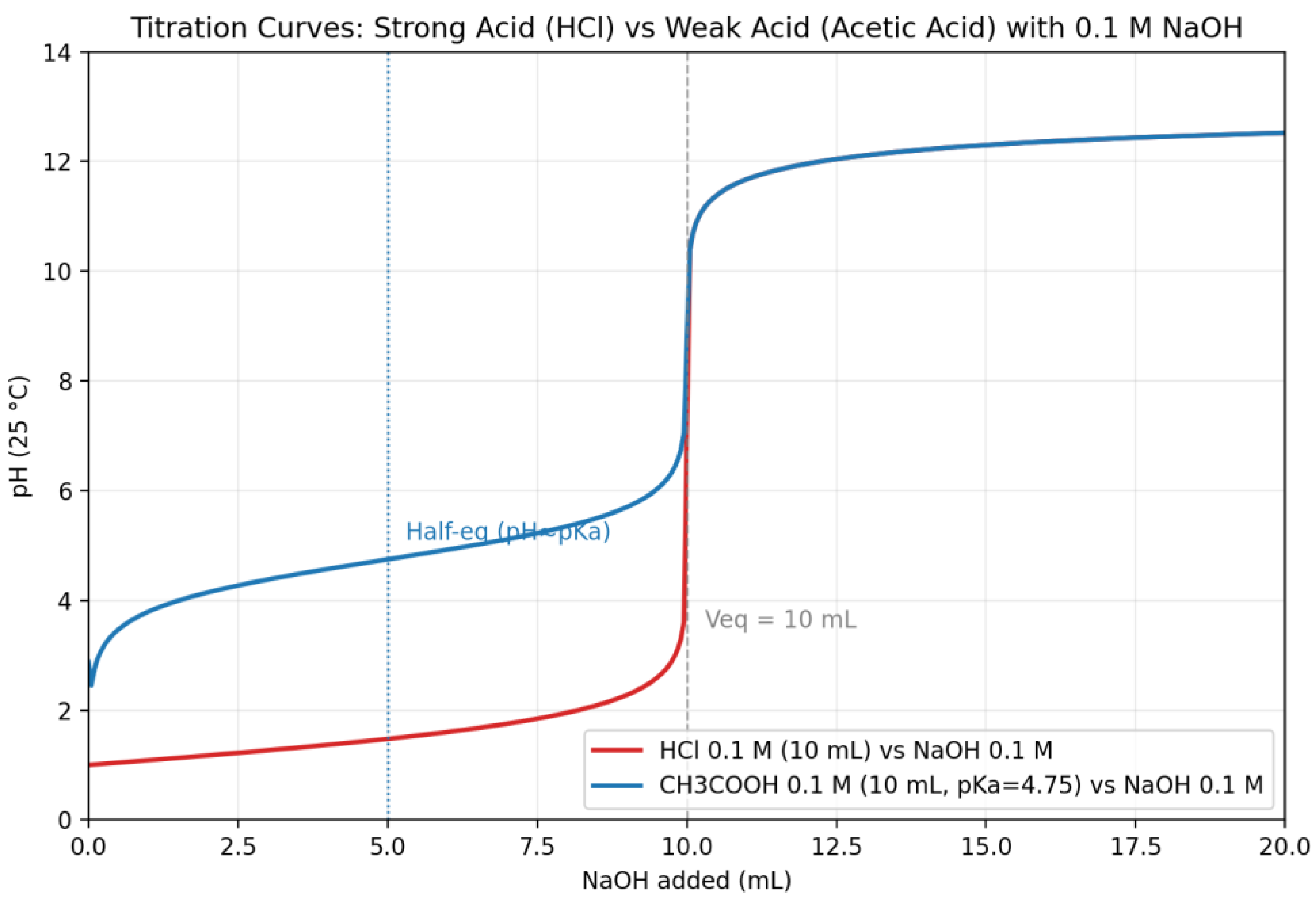
Figure 2.
Histograms and KDE for ACPP_FLN*ESYK (Linear Scale) Distribution of Light/Heavy ratios for the glycopeptide ACPP_FLN*ESYK in urine samples from prostate cancer patients. The left panel shows non-aggressive (NAG) cases, and the right panel shows aggressive (AG) cases. Histograms illustrate frequency distribution, while KDE (Kernel Density Estimation) curves provide a smooth representation of data density. Dashed lines indicate group medians.
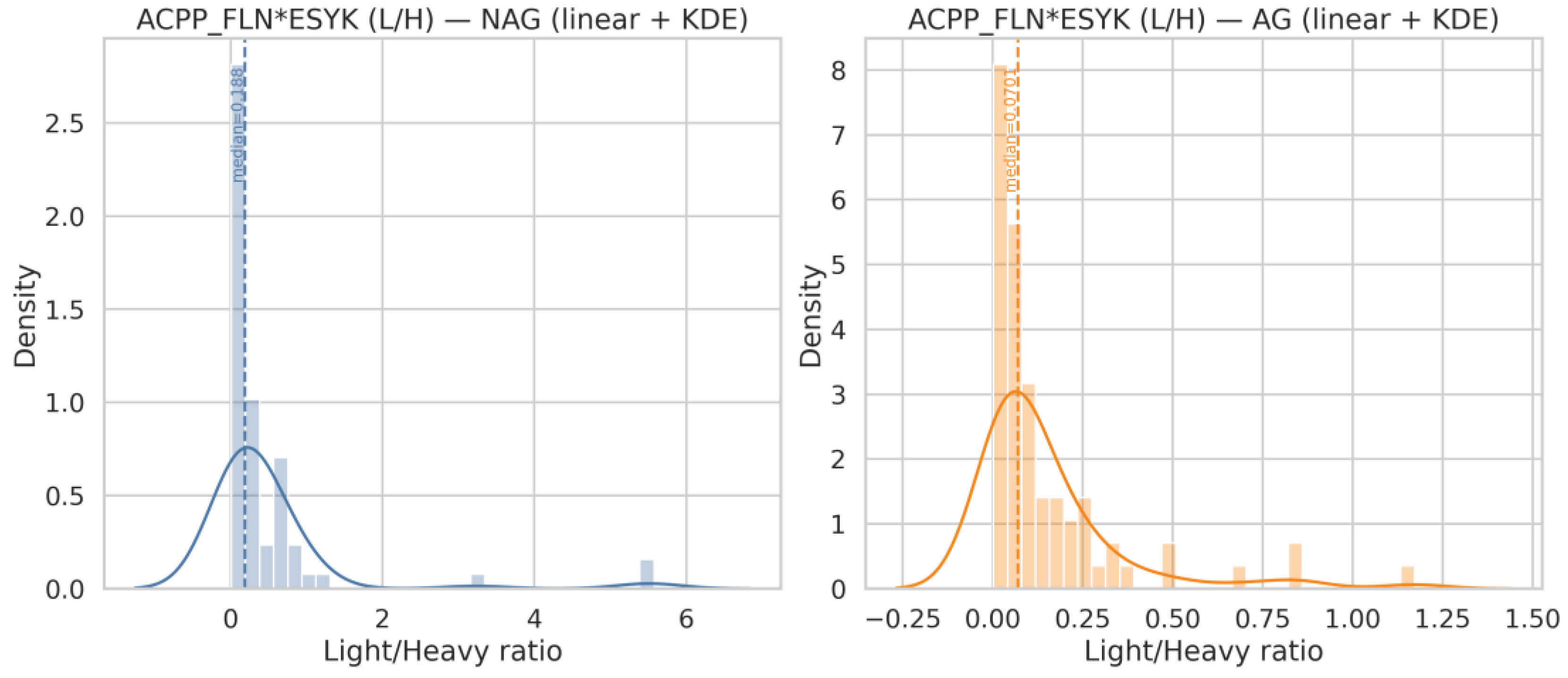
Figure 3.
Overlay of NAG and AG Distributions (Logarithmic Scale) Comparison of NAG and AG groups for ACPP_FLN*ESYK using log₁₀-transformed Light/Heavy ratios. Both histograms and KDE curves are overlaid on the same axis to highlight differences in distribution shape and central tendency between groups. Log scaling reduces skewness and emphasizes relative differences.
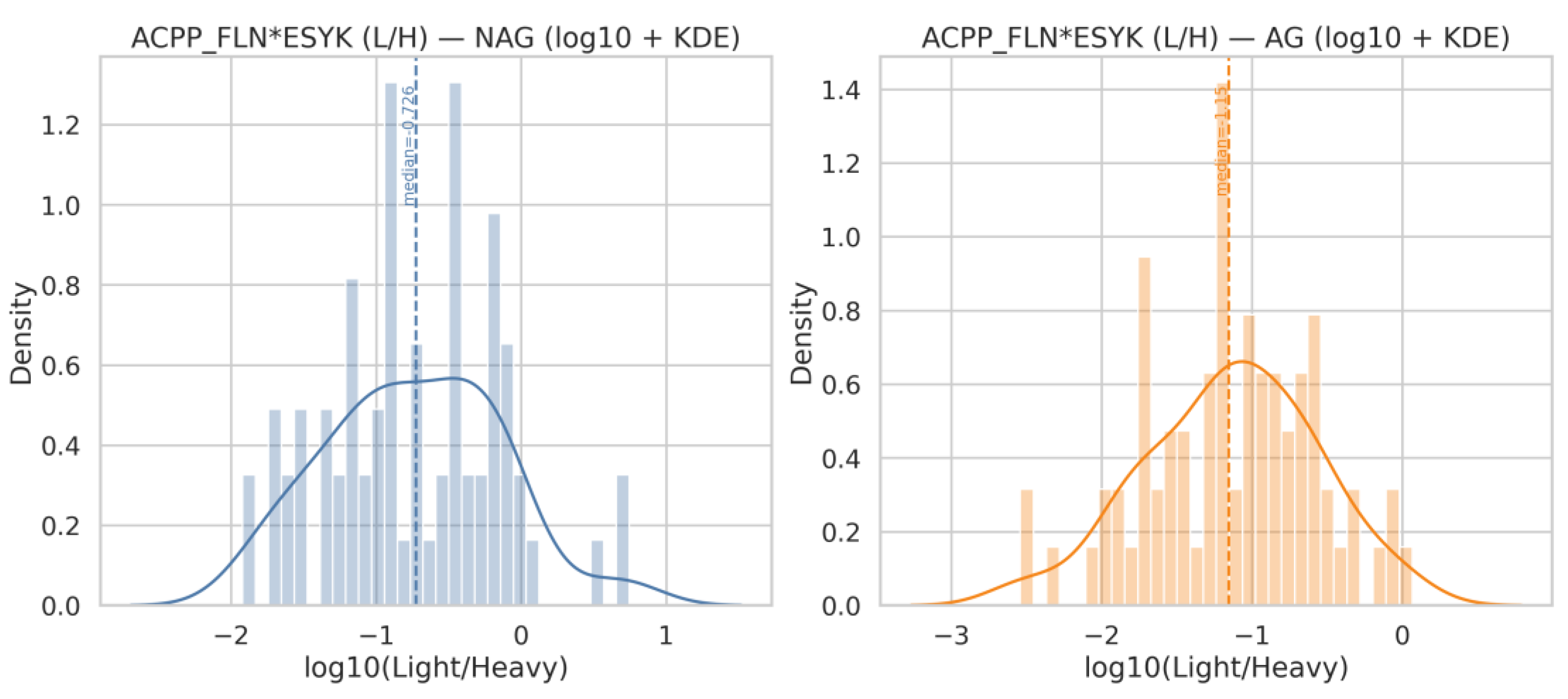
Figure 4.
Histograms and KDE for ACPP_FLN*ESYK (Logarithmic Scale) Distribution of log₁₀-transformed Light/Heavy ratios for ACPP_FLN*ESYK in urine samples. The left panel represents NAG, and the right panel represents AG cases. KDE curves reveal density peaks and spread, complementing histograms for visualizing skewed data.
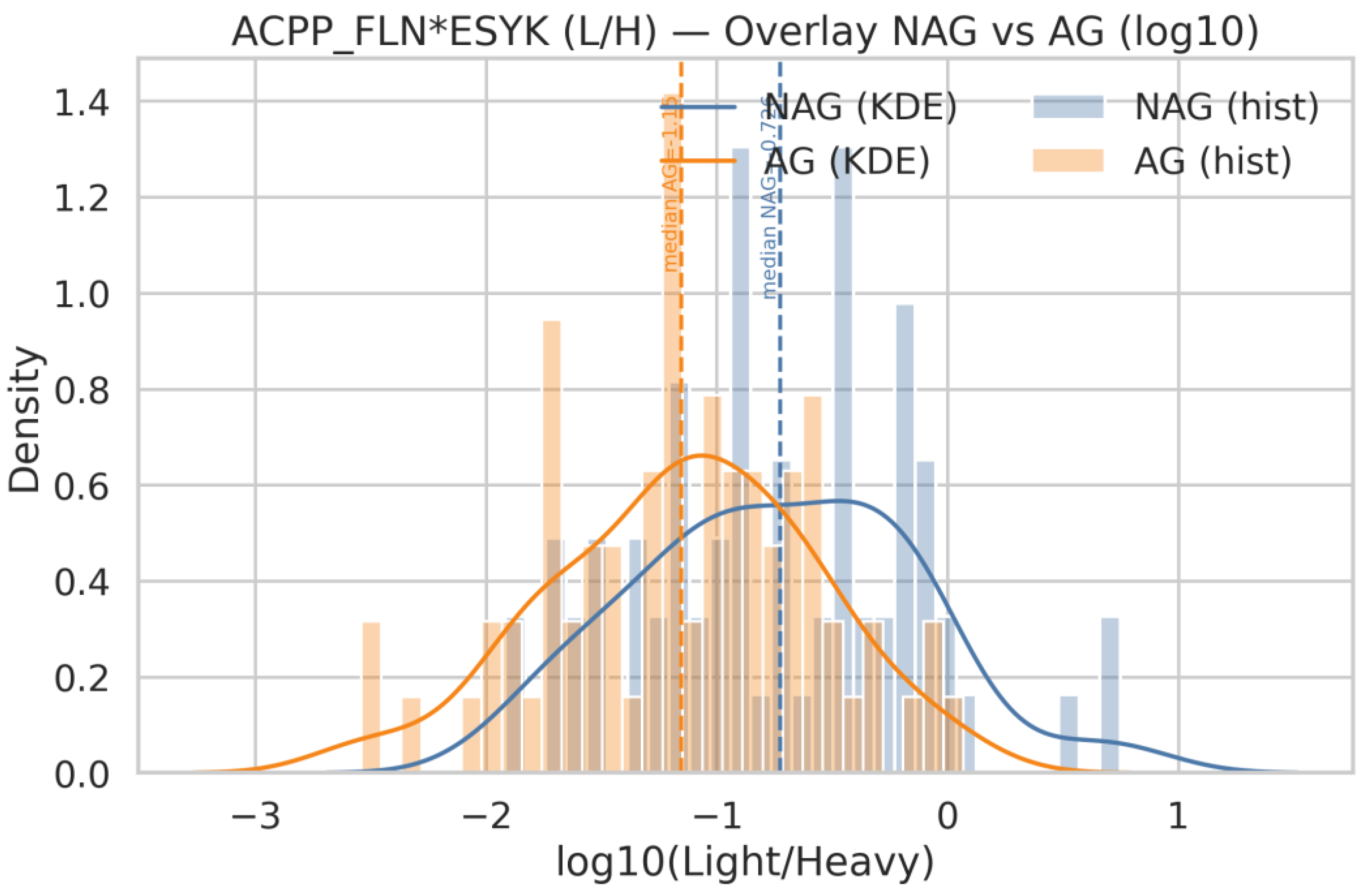
Figure 5.
CLU_EDALNETR Overlay (Linear Scale) Comparison of Light/Heavy ratios between NAG and AG groups using both histogram and kernel density estimation (KDE). The linear scale highlights distribution differences, with NAG shown in blue and AG in orange.
Figure 5.
CLU_EDALNETR Overlay (Linear Scale) Comparison of Light/Heavy ratios between NAG and AG groups using both histogram and kernel density estimation (KDE). The linear scale highlights distribution differences, with NAG shown in blue and AG in orange.
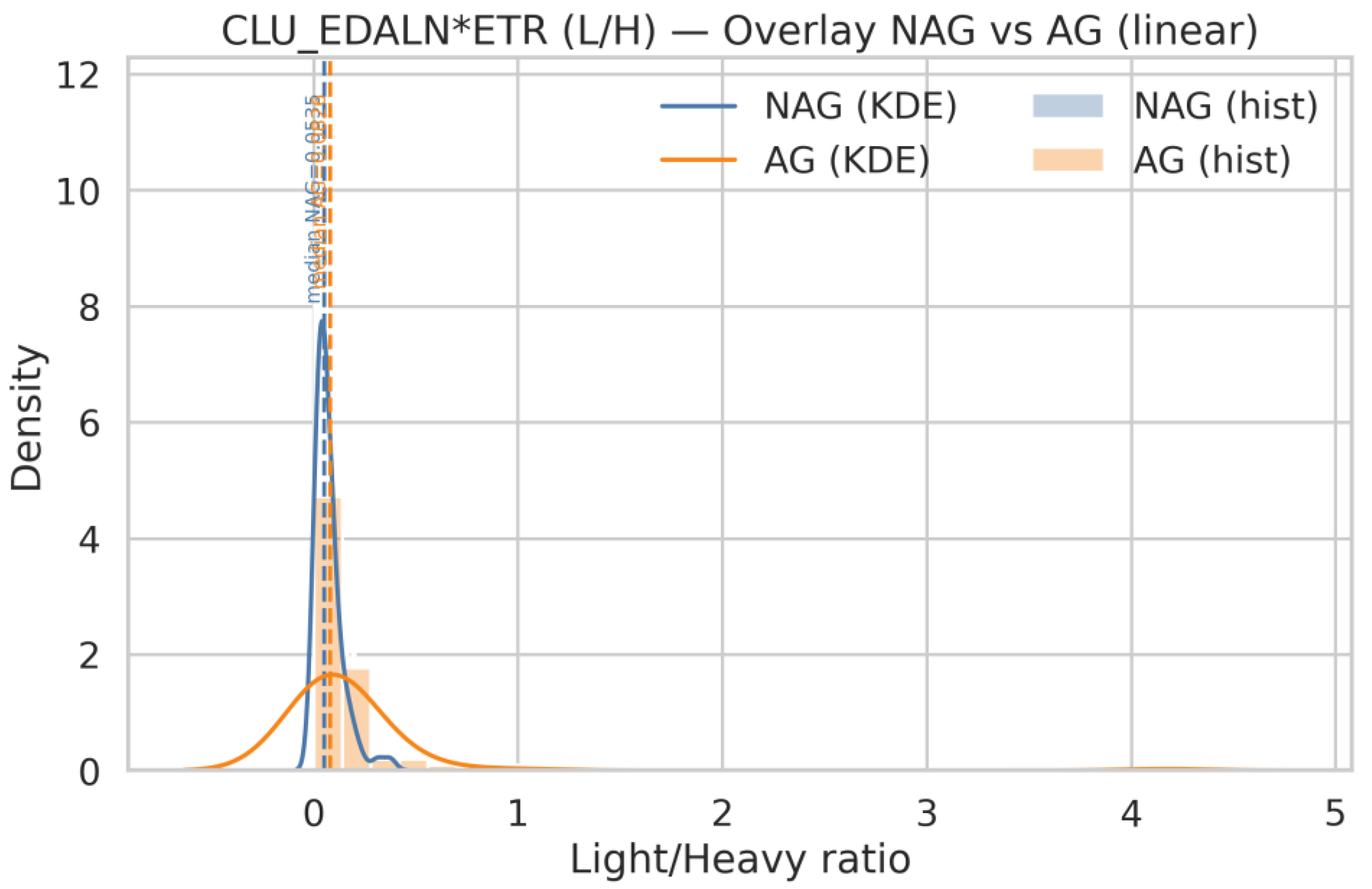
Figure 6.
CLU_EDALNETR Overlay (Logarithmic Scale) Log10-transformed Light/Heavy ratio comparison between NAG and AG groups. KDE and histogram overlays reveal distribution patterns with enhanced visibility of lower ratio values. NAG is represented in blue, AG in orange.
Figure 6.
CLU_EDALNETR Overlay (Logarithmic Scale) Log10-transformed Light/Heavy ratio comparison between NAG and AG groups. KDE and histogram overlays reveal distribution patterns with enhanced visibility of lower ratio values. NAG is represented in blue, AG in orange.
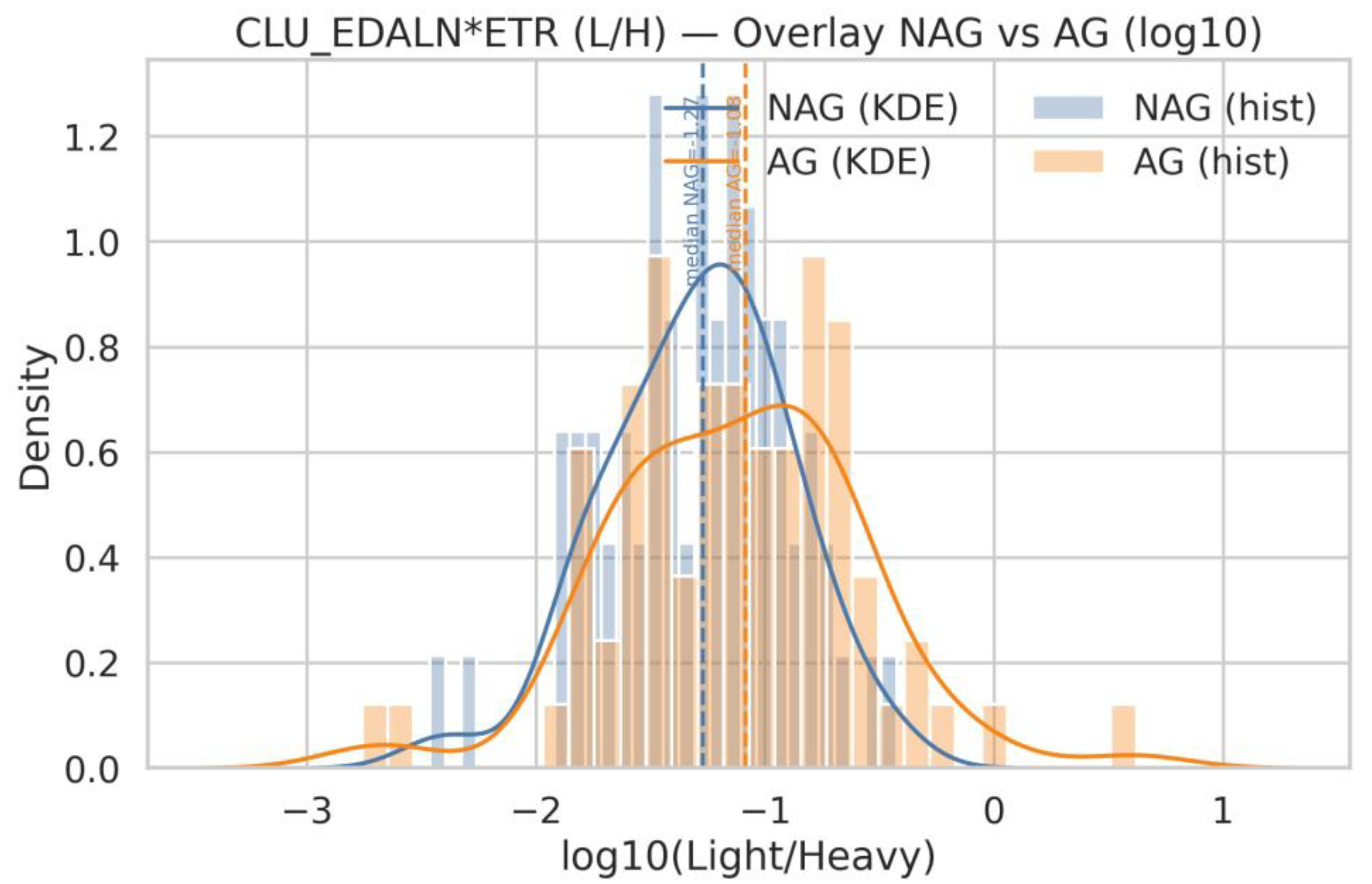
Figure 7.
Age distribution comparison between Non-Aggressive (NAG) and Aggressive (AG) groups, showing histograms, KDE curves, and median age markers.
Figure 7.
Age distribution comparison between Non-Aggressive (NAG) and Aggressive (AG) groups, showing histograms, KDE curves, and median age markers.
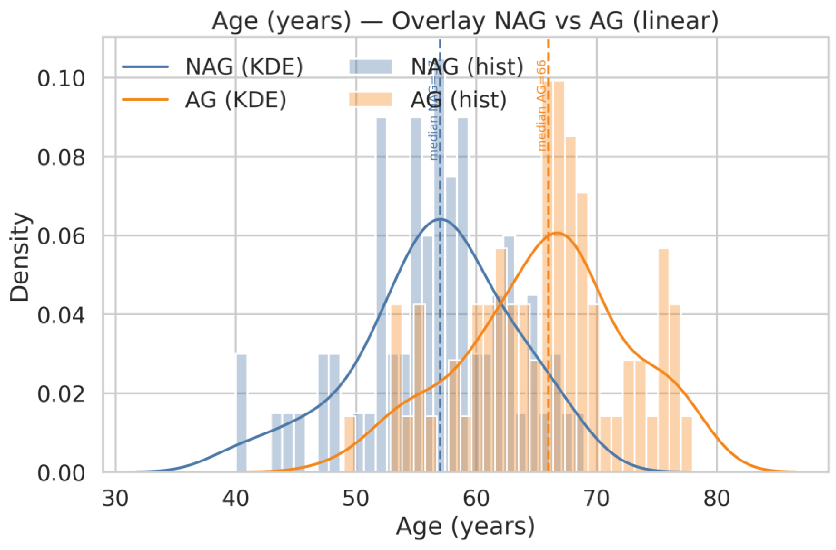
Figure 8.
Distribution of serum PSA levels (log10 scale) in Non-Aggressive (NAG) and Aggressive (AG) groups, showing histograms, KDE curves, and median markers.
Figure 8.
Distribution of serum PSA levels (log10 scale) in Non-Aggressive (NAG) and Aggressive (AG) groups, showing histograms, KDE curves, and median markers.
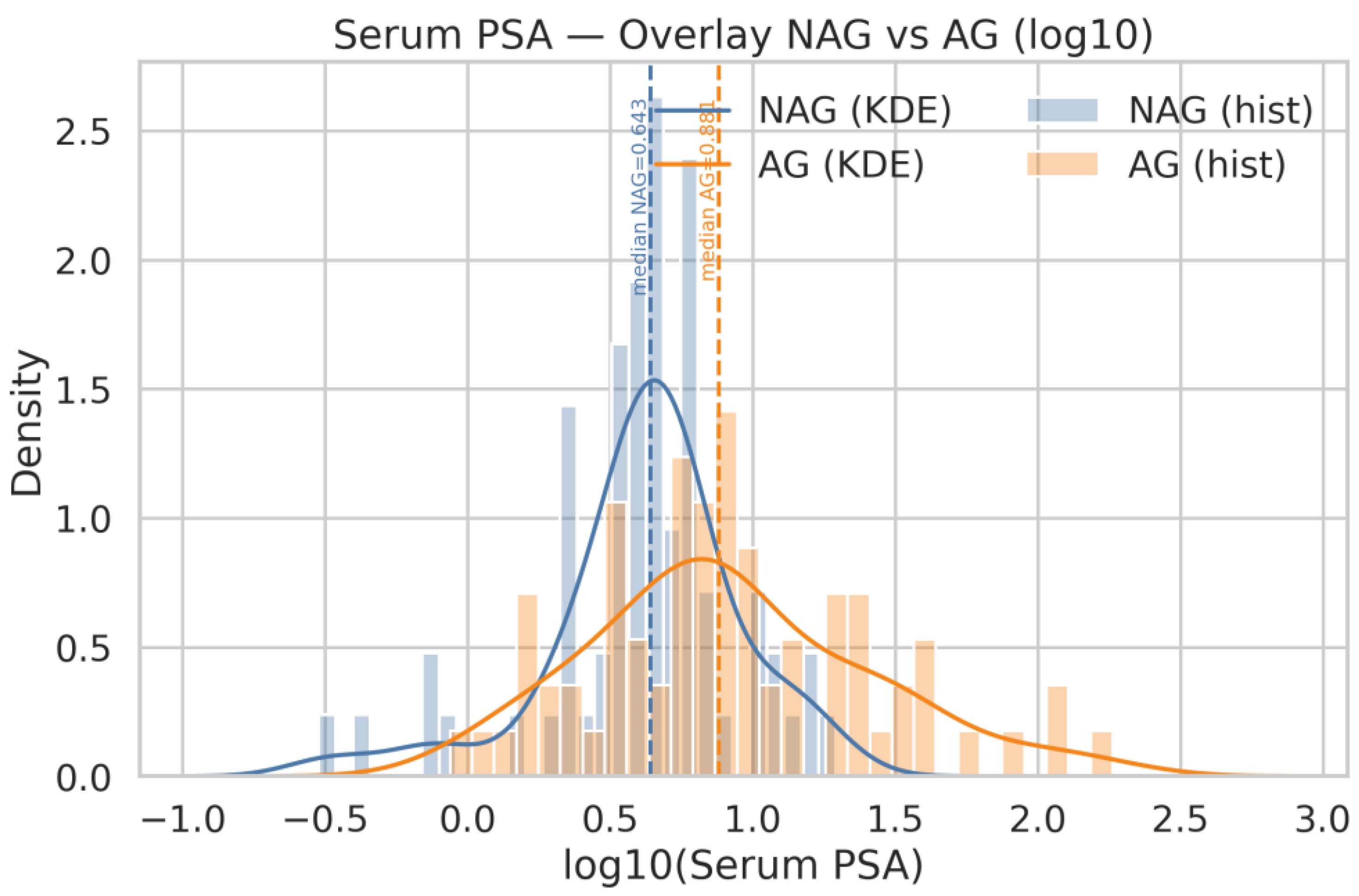
Figure 9.
Comparison of ACPP_FLN*ESYK expression between non-aggressive (NAG) and aggressive (AG) prostate cancer groups using box plots. (a) Raw scale values with effect size and significance (Welch t p = 8.06×10⁻³; Mann–Whitney p = 1.85×10⁻⁴; Cohen’s d = –0.47). (b) Log-transformed values showing improved separation (Welch t p = 6.53×10⁻⁵; Mann–Whitney p = 1.85×10⁻⁴; Cohen’s d = 0.69).
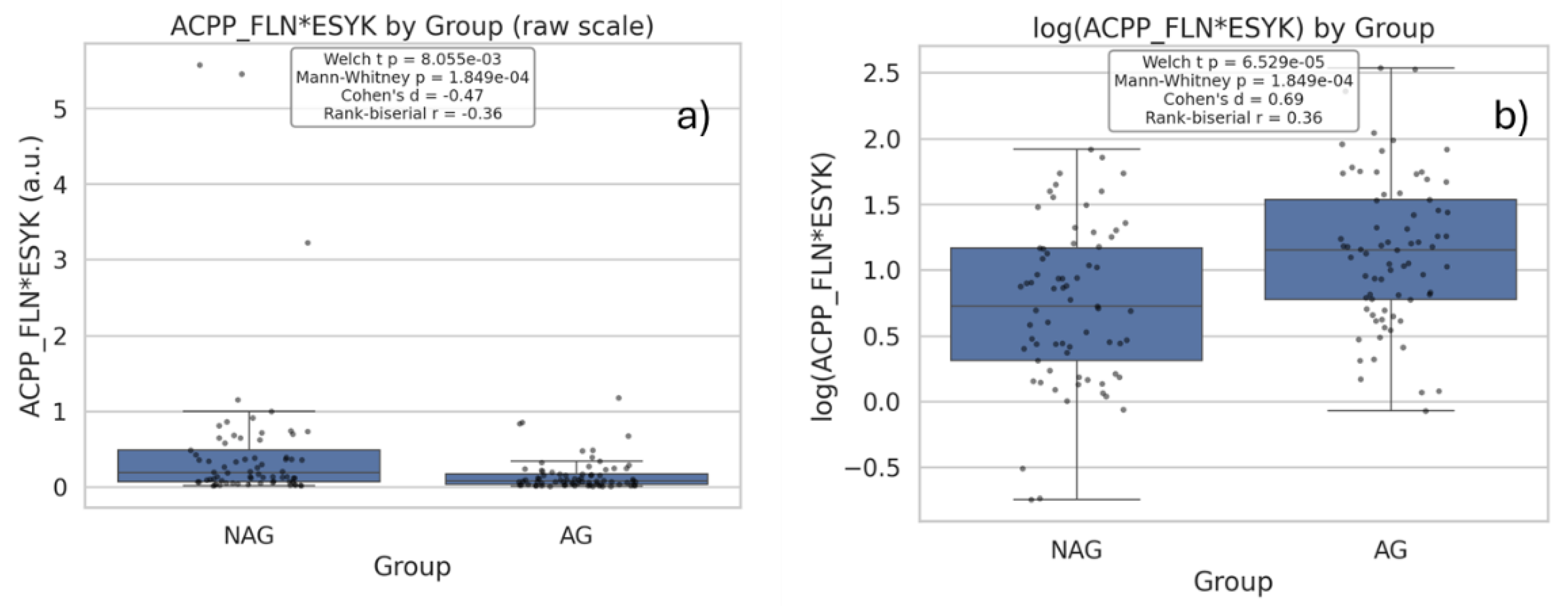
Figure 10.
Comparison of CLU_EDALN*ETR expression between non-aggressive (NAG) and aggressive (AG) prostate cancer groups using box plots. (a) Raw scale values with statistical results (Welch t p = 6.79×10⁻²; Mann–Whitney p = 3.38×10⁻²; Cohen’s d = 0.30). (b) Log-transformed values showing reversed effect direction (Welch t p = 3.67×10⁻²; Mann–Whitney p = 3.38×10⁻²; Cohen’s d = –0.35).
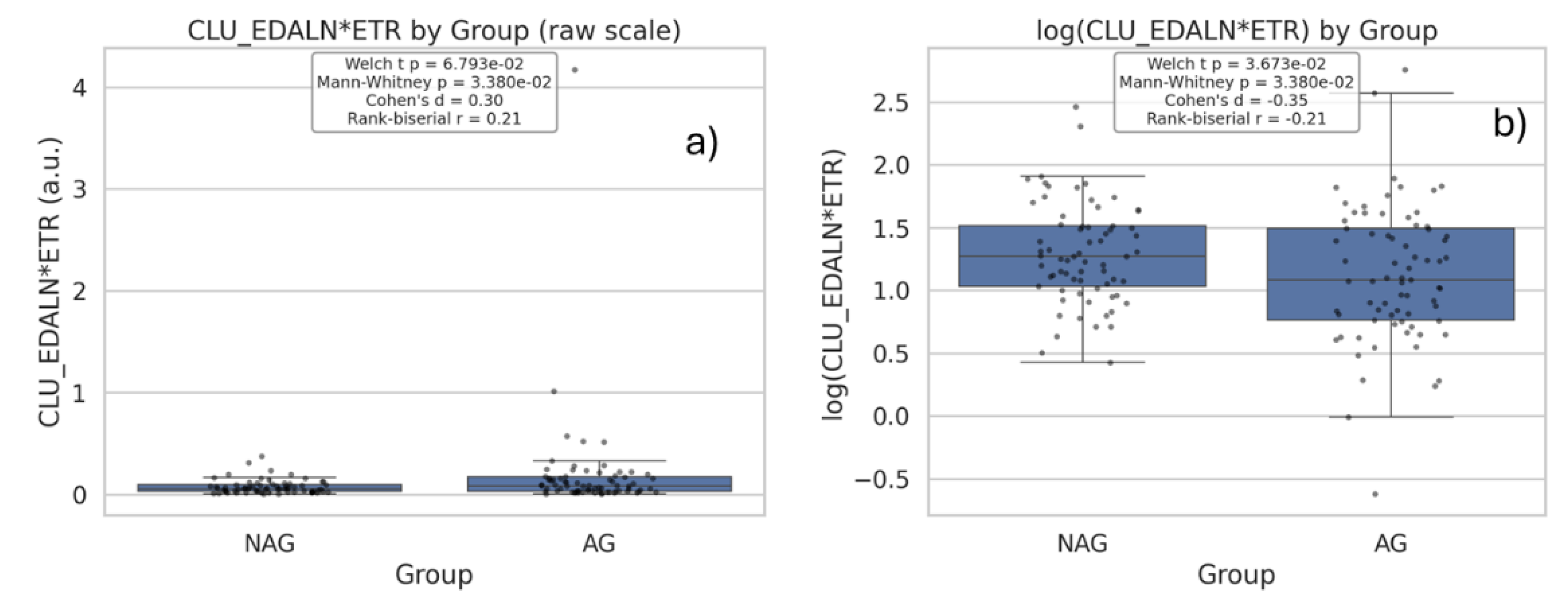
Figure 11.
Comparison of age and serum PSA between non-aggressive (NAG) and aggressive (AG) prostate cancer groups using box plots. (a) Age shows a significant difference (Welch t p = 7.72×10⁻¹⁴; Cohen’s d = 1.39). (b) Serum PSA (log₁₀ scale) also differs significantly (Welch t p = 4.52×10⁻⁵; Cohen’s d = 0.70.
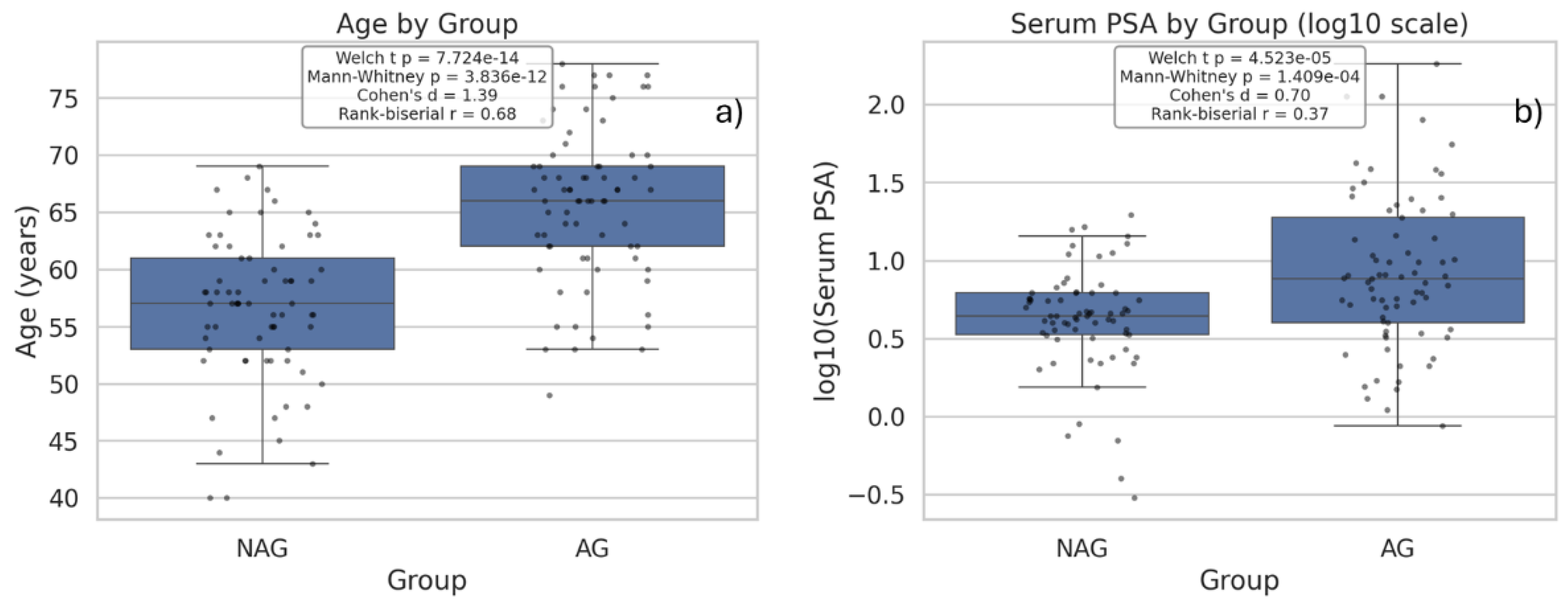
Figure 12.
Correlation between ACPP_FLNESYK and CLU_EDALNETR in prostate cancer groups on a log10–log10 scale. (a) NAG group: n = 69; Pearson r = 0.525 (p < 0.001); Spearman ρ = 0.548 (p < 0.001); R² = 0.276. (b) AG group: n = 73; Pearson r = 0.740 (p < 0.001); Spearman ρ = 0.704 (p < 0.001); R² = 0.548. Regression lines indicate positive associations in both groups, stronger in AG.
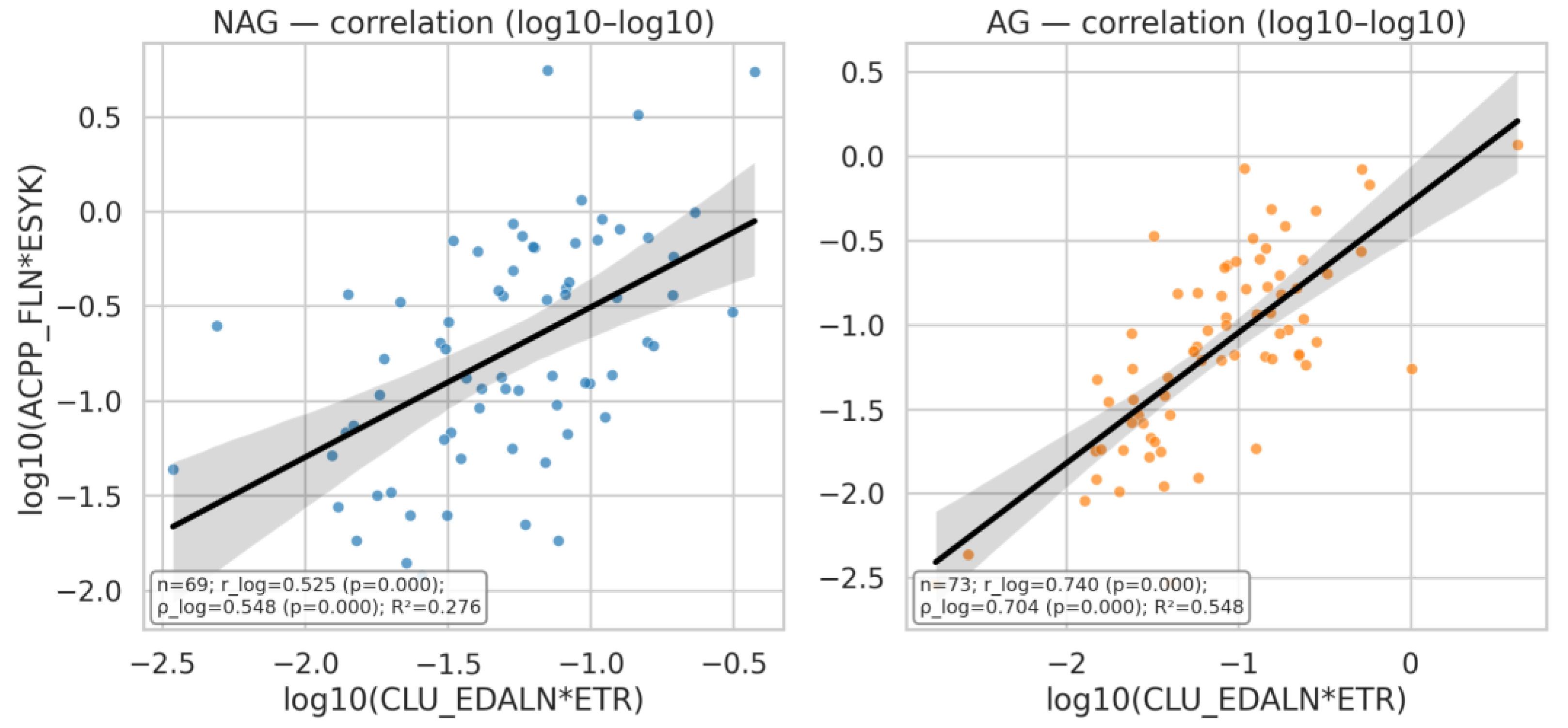
Figure 13.
Comparison of log(ACPP_FLN*ESYK) between non-aggressive (NAG) and aggressive (AG) prostate cancer groups using box plots. Statistical results: Welch t p = 6.53×10⁻⁵; Mann–Whitney p = 1.85×10⁻⁴; Cohen’s d = 0.69; Rank-biserial r = 0.36.
Figure 13.
Comparison of log(ACPP_FLN*ESYK) between non-aggressive (NAG) and aggressive (AG) prostate cancer groups using box plots. Statistical results: Welch t p = 6.53×10⁻⁵; Mann–Whitney p = 1.85×10⁻⁴; Cohen’s d = 0.69; Rank-biserial r = 0.36.
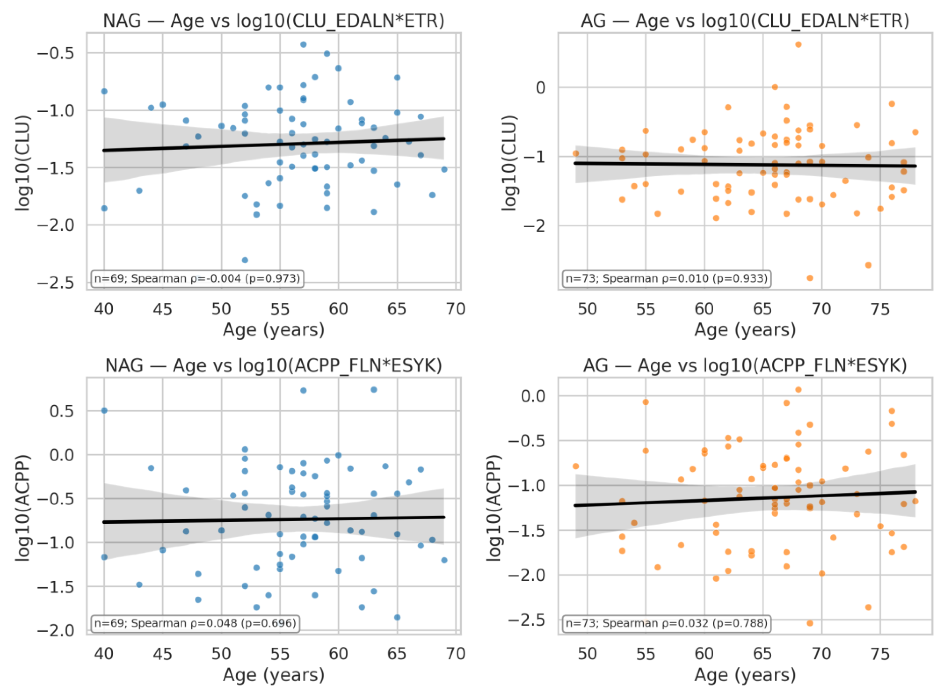
Figure 14.
PCA Score Plot (PC1 vs. PC2) for the Physicochemical Properties of Chemical Elements. Elements are labeled with their atomic symbols and are color- and shape-coded according to their group in the periodic table (Groups 1-18). PC1 explains 43.8% of the total variance in the data.
Figure 14.
PCA Score Plot (PC1 vs. PC2) for the Physicochemical Properties of Chemical Elements. Elements are labeled with their atomic symbols and are color- and shape-coded according to their group in the periodic table (Groups 1-18). PC1 explains 43.8% of the total variance in the data.
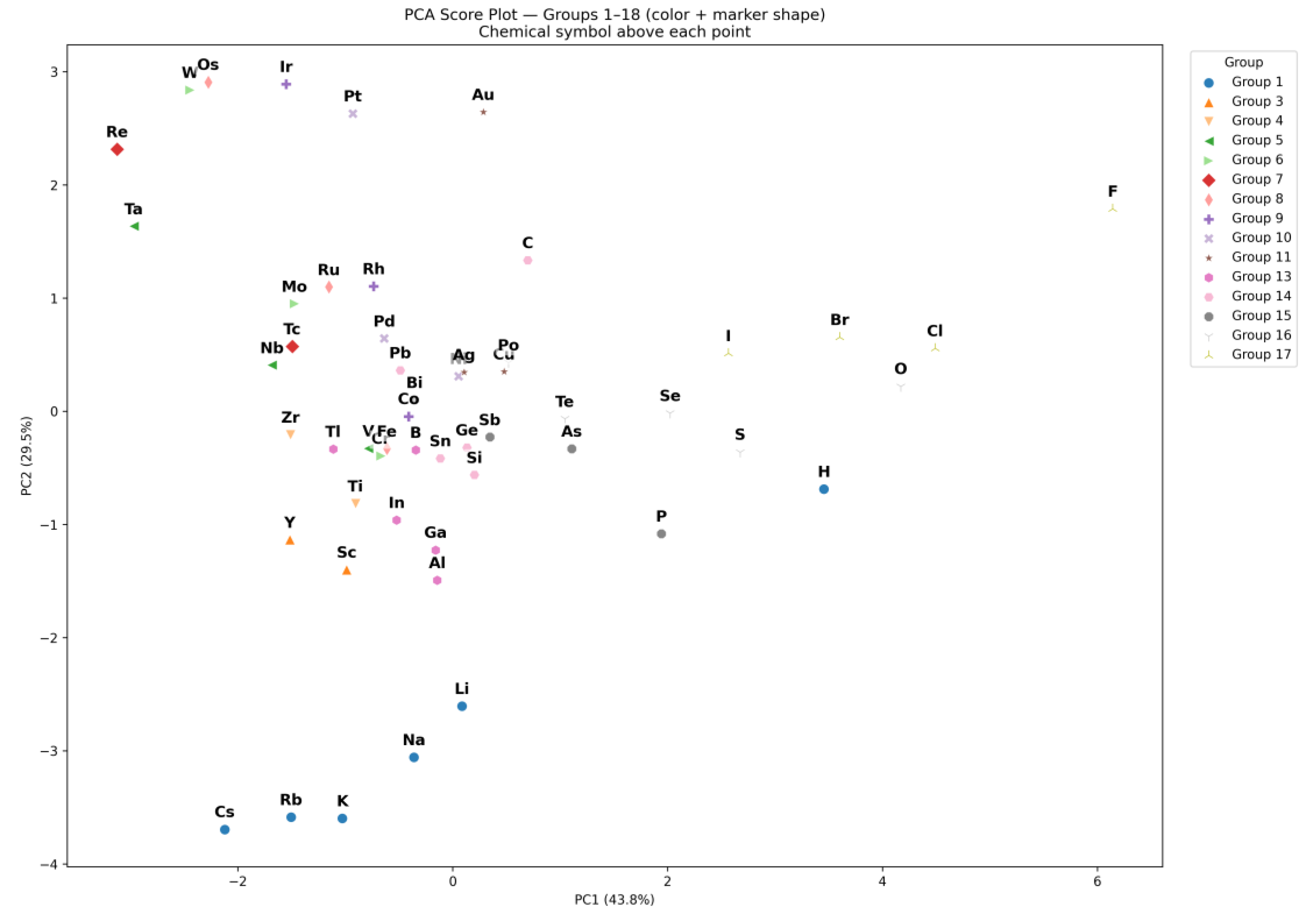
Figure 15.
Loading plot (correlation circle) from the Principal Component Analysis (PCA) of physicochemical properties of periodic table elements.
Figure 15.
Loading plot (correlation circle) from the Principal Component Analysis (PCA) of physicochemical properties of periodic table elements.
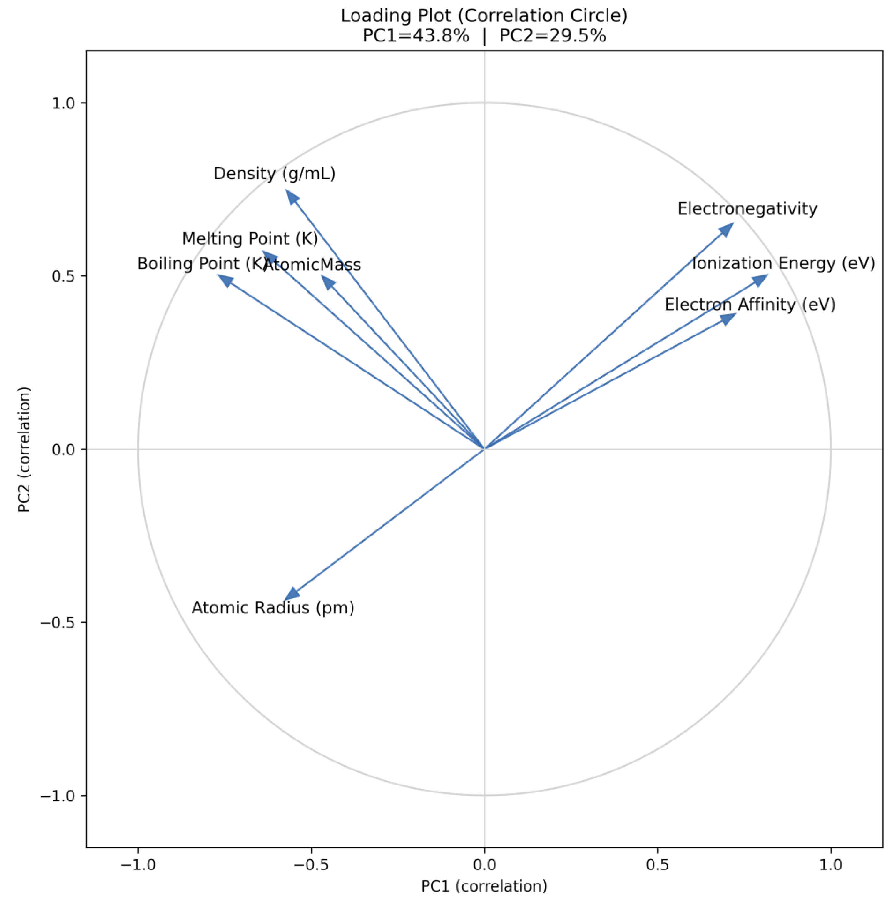
Figure 16.
Plotted the heatmap with a diverging color scale centered at 0 (blue = negative, white = near zero, red = positive), annotated with the r coefficients.
Figure 16.
Plotted the heatmap with a diverging color scale centered at 0 (blue = negative, white = near zero, red = positive), annotated with the r coefficients.
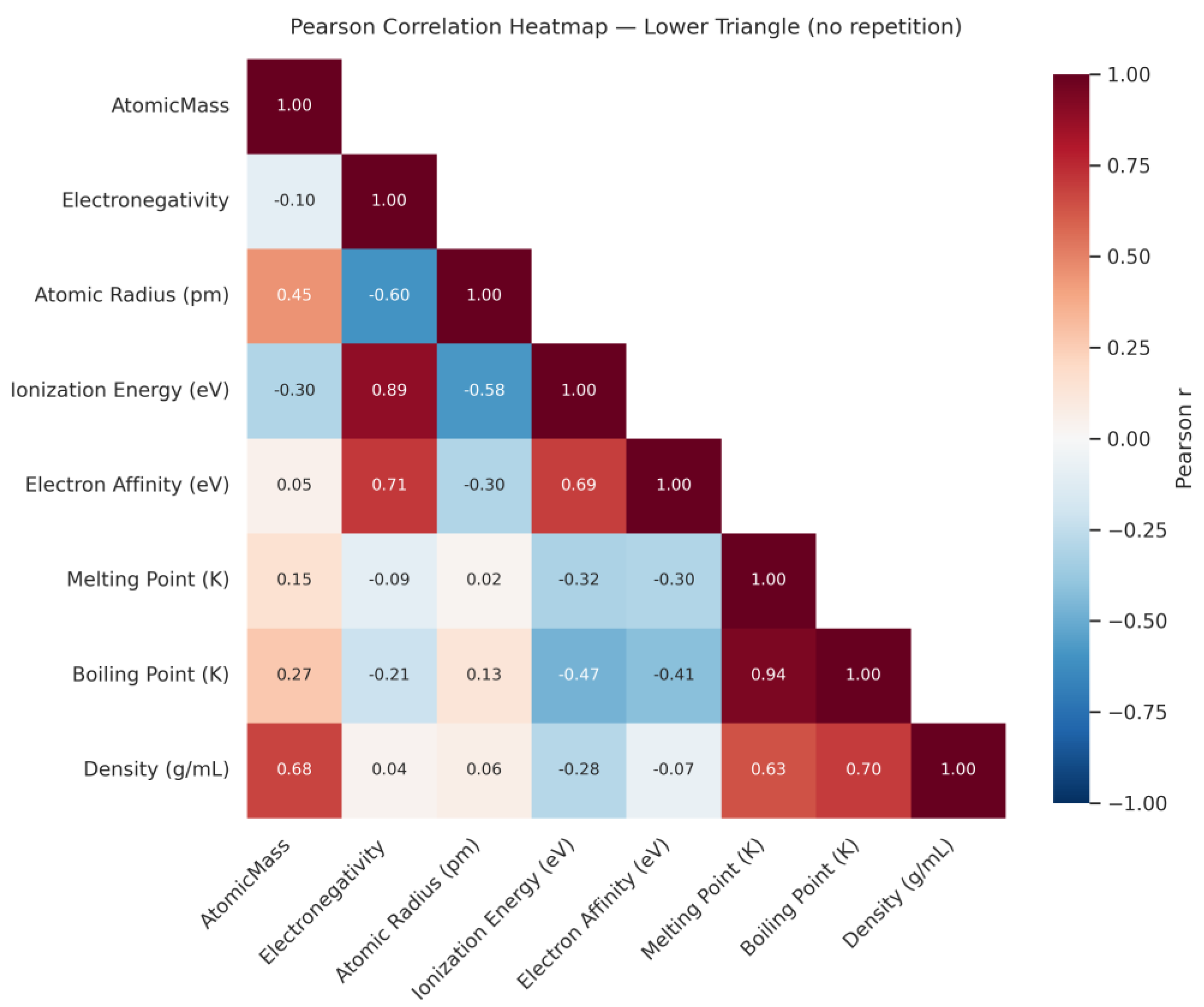
Figure 20.
Pairwise comparison of eight key properties—Atomic Mass, Electronegativity, Atomic Radius, Ionization Energy, Electron Affinity, Melting Point, Boiling Point, and Density—across three chemical groups (Nonmetal, Metal, Metalloid).
Figure 20.
Pairwise comparison of eight key properties—Atomic Mass, Electronegativity, Atomic Radius, Ionization Energy, Electron Affinity, Melting Point, Boiling Point, and Density—across three chemical groups (Nonmetal, Metal, Metalloid).
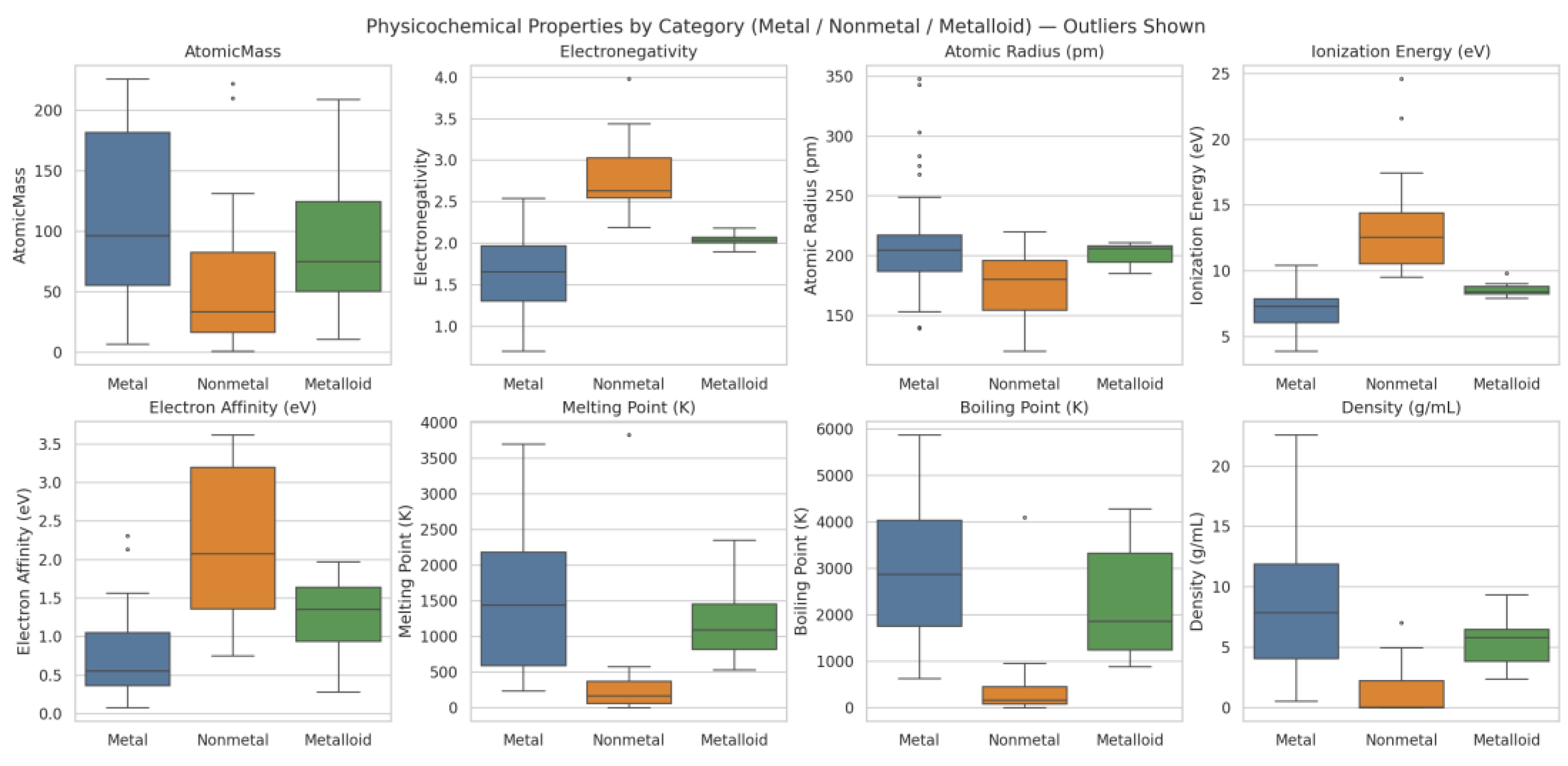
Figure 21.
a) Water density determined by students during a general chemistry laboratory class, b) box plot generated of the obtained data using Copilot.
Figure 21.
a) Water density determined by students during a general chemistry laboratory class, b) box plot generated of the obtained data using Copilot.
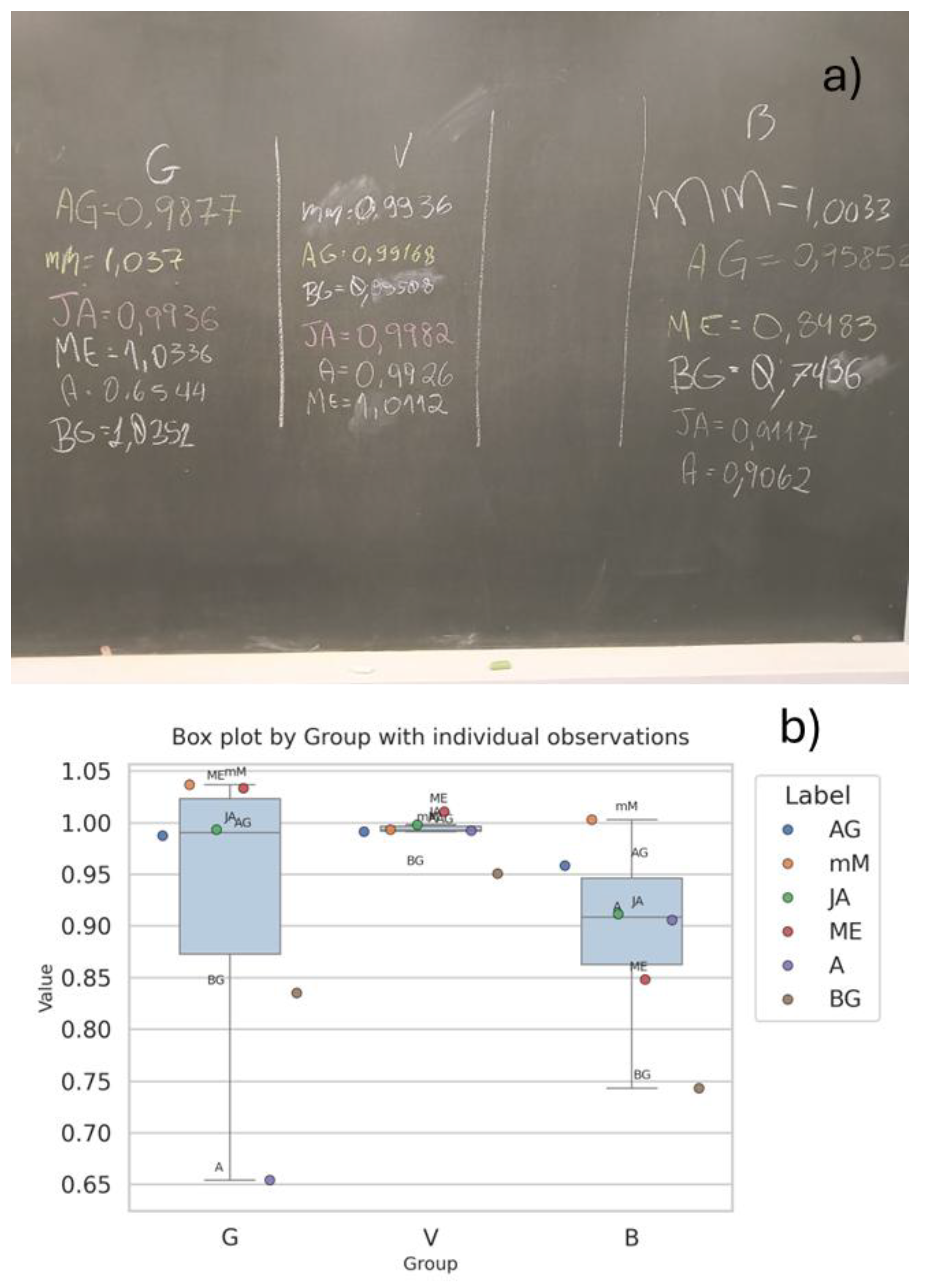

Table 1.
Representative Chemistry and Data Analysis Tasks Used to Evaluate Copilot’s Performance Questions Q1–Q16 cover fundamental chemical equilibrium, acid–base calculations, and titrations, while Q17–Q32 address visualization and statistical analysis tasks, including histograms, box plots, correlation plots, PCA, and heatmaps.
| Questions | Task |
| Q1 | Calculate the amount of ethyl ethanoate formed when 2 moles of ethanoic acid and 3 moles of ethanol and 8 moles of water are allowed to come to equilibrium. The equilibrium constant for the reaction is 3.0. |
| Q2 | Calculate the pH of 0.025 M HI |
| Q3 | Calculate the pH of 0.025 M Sr(OH)₂ |
| Q4 | Calculate the pH of 2.0 M HF. Ka for HF = 6.6 × 10⁻⁴ |
| Q5 | Calculate the pH of 2.0 M CH₃NH₂. Kb for CH₃NH₂ = 4.38 × 10⁻⁴ |
| Q6 | Calculate the pH of 0.25 M NH₄Cl. Kb for NH₃ = 1.8 × 10⁻⁵ |
| Q7 | Calculate the pH of 0.25 M NaF. Ka for HF = 6.6 × 10⁻⁴ |
| Q8 | How many mL of 0.20 M KOH are needed to neutralize 150 mL of 0.020 M H₂SO₄? |
| Q9 | How many mL of 0.20 M HCl are needed to neutra lize 150 mL of 0.020 M Ca(OH)₂? |
| Q10 | If 25.0 mL of 0.25 M HNO₃ is combined with 15.0 mL of 0.25 M CH₃NH₂, what is the pH? Kb = 4.38 × 10⁻⁴ |
| Q11 | : If 25.0 mL of 0.25 M NaOH is combined with 15.0 mL of 0.25 M CH₃COOH, what is the pH? Ka = 1.8 × 10⁻⁵ |
| Q12 | A household cleaner contains ammonia. A 25.37 g sample of the cleaner is dissolved in water and made up to 250 cm3. A 25.0 cm3 portion of this solution requires 37.3 cm3 of 0.360 mol dm-3 sulfuric acid for neutralization. What is the percentage by mass of ammonia in the cleaner? |
| Q13 | 8.492 g of Ammonium iron (II) sulphate crystals ((NH4)2SO4.FeSO4.nH2O) were dissolved in water and the solution was made up to 250 cm3 with distilled water and diluted sulphuric acid. A 25.0 cm3 portion of the solution was further acidified and titrated against potassium permanganate (VII) solution of concentration 0.0150 mol dm-3, requiring 22.5 cm3 for neutralization to be achieved. Determine the value of n. |
| Q14 | An aspirin tablet was ground using a glass rod, and 25 mL of a 1.0 mol/L NaOH solution was added to the powder. The mixture was then heated for 15 minutes to ensure complete reaction. After cooling, the excess NaOH was titrated with 20 mL of a 0.5 mol/L H₂SO₄ solution. Based on this data, calculate the mass of aspirin present in the tablet. (Molar mass of aspirin = 180.1574 g/mol). The aspirin was neutralized by NaOH, the, it was hydrolyzed to salicylic acid |
| Q15 | How many moles of sodium ethanoate must be added to 1.00 dm3 of 0.0100 mol dm-3 of ethanoic acid to produce a buffer solution of pH 5.8? |
| Q16 | : Calculate the pH of the following solutions: a) HCl, 0.1 mol/L b) Acetic acid, 0.1 mol/L (pKa = 4.75) c) How many times is the [H⁺] concentration in the HCl solution greater than that in the acetic acid solution? |
| Q17 | .For 10 mL of HCl (0.1 mol/L) and 10 mL of acetic acid (0.1 mol/L, pKa = 4.75), each titrated with NaOH (0.1 mol/L).Present both titration curves on the same graph for comparison. |
| Load the spreadsheet 1 | |
| Q18 | Generate histograms for ACPP_FLN*ESYK (Light/Heavy) and, split by AG and NAG groups. Display both linear and logarithmic scales, include KDE (kernel density estimation) curves, and overlay the NAG and AG distributions on the same axis for comparison |
| Q19 | Show same for CLU_EDALN*ETR |
| Q20 | Show the same for age and Serum PSA |
| Q21 | Compare the expression levels of the glycopeptide ACPP_FLN*ESYK between aggressive (AG) and nonaggressive (NAG) prostate cancer groups using box plots. |
| Q22 | Compare the expression levels of the glycopeptide CLU_EDALN*ETR between aggressive (AG) and nonaggressive (NAG) prostate cancer groups using box plots |
| Q23 | Compare age and serum PSA between aggressive (AG) and nonaggressive (NAG) prostate cancer groups using box plots |
| Q24 | Build a correlation plot of ACPP_FLN*ESYK (y-axis) vs CLU_EDALN*ETR (x-axis), with the data split by AG and NAG groups |
| Q25 | : Build a correlation plot of age vs ACPP_FLN*ESYK (y-axis) and CLU_EDALN*ETR (x-axis), with the data split by AG and NAG groups |
| Upload Spreadsheet 2 | |
| Q26 | Generate a score plot showing the distribution of different physicochemical properties (e.g., atomic radius, electronegativity, ionization energy) for the elements in the periodic table. |
| Q27 | Generate a PCA loading plot to display the relationship between variables and principal components, highlighting their contributions and directions |
| Q28 | Create a Pearson correlation heatmap showing the relationships between the physicochemical properties of the elements in the periodic table |
| Q29 | Construct a correlation plot comparing the Boiling Point and Melting Point of elements. |
| Q30 | Construct a correlation plot comparing Ionization Energy and Electron Affinity of elements |
| Q31 | Construct a correlation plot comparing Ionization Energy and Electronegativity of elements. |
| Q32 | Does a comparison of physicochemical properties among groups (Column E; metals, nonmetals, and metalloids) using box plot, show all the box plots in the same image |
Table 2.
ICE table built by Copilot.
| Species | Initial (moles) | Change (moles) | Equilibrium (moles) |
| CH3COOH | 2 | -x | 2 - x |
| CH3CH2OH | 3 | -x | 3 - x |
| CH3COOCH2CH3 | 0 | +x | x |
| H2O | 8 | +x | 8 + x |
Disclaimer/Publisher’s Note: The statements, opinions and data contained in all publications are solely those of the individual author(s) and contributor(s) and not of MDPI and/or the editor(s). MDPI and/or the editor(s) disclaim responsibility for any injury to people or property resulting from any ideas, methods, instructions or products referred to in the content. |
© 2025 by the authors. Licensee MDPI, Basel, Switzerland. This article is an open access article distributed under the terms and conditions of the Creative Commons Attribution (CC BY) license (http://creativecommons.org/licenses/by/4.0/).
Copyright: This open access article is published under a Creative Commons CC BY 4.0 license, which permit the free download, distribution, and reuse, provided that the author and preprint are cited in any reuse.


