
Submitted:
14 October 2025
Posted:
15 October 2025
You are already at the latest version
Abstract
Close formation flight is a practical strategy for fixed-wing unmanned aerial vehicle (UAV) swarms. Maintaining UAVs at aerodynamically optimal positions is essential for efficient formation flight. However, aerodynamic optimization methods based on computational fluid dynamics (CFD) are computationally intensive and difficult to apply in real time for large-scale formations. Inspired by bio-formation flight, this study proposes an on-board sensing-based method for wake flow field estimation, with potential for extension to complex formations. The method is based on a parameter identification-induced velocity model (PI-Model), which uses only onboard sensors, including two lateral air data systems (ADS), to sample the wake field. By minimizing the residual of the induced velocity, the model identifies key parameters of the wake and provides a dynamic estimation of the wake velocity field. Comparisons between the PI-Model and CFD simulations show that it achieves higher accuracy than the widely used single horseshoe vortex model in both wake velocity and aerodynamic effects. Applied to a two-UAV formation scenario, CFD validation confirms that the trailing UAV achieves a 15%–25% drag reduction. These results verify the effectiveness of the proposed method for formation flight and demonstrate its potential for application in complex, dynamic multi-UAV formations.
Keywords:
formation flight
; wake vortex modeling
; on-board sensing
1. Introduction
V-shaped and line-formation are commonly observed during migratory bird flights [1,2]. Numerous studies have shown that such formations significantly reduce individual energy expenditure and improve endurance. Further observations indicate that individuals adaptively adjust their positions relative to leading neighbors to maximize energy savings [3]. This efficient coordination mechanism provides a clear direction for bio-inspired aviation: translating it into close formation flight in engineering applications. When properly positioned within the leader's upwash field, the follower experiences a forward-inclined lift vector, reducing induced drag and enhancing aerodynamic performance [4]. These benefits have been confirmed through theoretical analysis [5], wind tunnel experiments [6], and flight tests [7].
As a result, close formation flight has rapidly become a central focus in UAV formation research in recent years [8,9,10,11,12,13,14,15]. The primary challenge lies in determining the aerodynamically optimal relative positions [16]. For larger formations, constructing wake databases using CFD provides high accuracy [17,18], but its reliance on large data volumes, computational resources, and airframe consistency limits its scalability to multi-aircraft and cross-platform applications. In our previous work, we introduced the concept of “formation unit” [19], aiming to address multi-UAV formations within an optimization framework. However, in heterogeneous and complex formation scenarios, the limitations of this approach have gradually become evident.
Achieving this goal relies on constructing a formation aerodynamic model that is both accurate and efficient. Existing analytical studies span several theoretical frameworks, including the single horseshoe vortex model [20,21], multiple horseshoe vortex models [22], and vortex lattice methods [23,24], with new modeling approaches also emerging in recent years [25,26]. In general, the single horseshoe vortex model offers high computational efficiency, while vortex lattice methods provide higher accuracy but are limited by the real-time requirements of online computation. In realistic environments, however, wake vortices are influenced by various factors, including maneuvers of the leading aircraft and external disturbances such as stochastic wind fields, resulting in time-varying wake characteristics [27,28]. If static, pre-calibrated model parameters are still used, the system cannot update wake information in real time, making it difficult to accurately predict the strength and position of the upwash region experienced by the follower aircraft. As a result, the energy-saving benefits cannot be sustained. Therefore, to consistently achieve drag reduction in operational scenarios, the system must be capable of continuously sensing and updating wake information—i.e., wake tracking.
Wake tracking is not a new concept, but most existing studies focus on hazardous wake vortex warning and avoidance in civil aviation [29,30]. Direct wake flow measurements typically rely on on-board LiDAR systems [31,32] or ground-based acoustic devices [33]. Although ground-based measurements have achieved reliable results [34], transferring these methods to on-board platforms remains challenging [35]. An alternative approach involves indirect parameter estimation. For example, in Ref. [36], distributed pressure sensors are mounted on the follower’s wing, and an extended Kalman filter (EKF) is used to estimate wake vortex parameters. This method performs well across various configurations, particularly in vortex localization; however, it suffers from limited observability [37] and requires additional sensors, which increases cost and imposes design constraints. These challenges lead us to consider whether it is possible to extract critical wake features in real time without relying on heavy and expensive equipment, by fully utilizing existing or lightweight additional on-board sensors, to enable more accurate aerodynamic modeling.
Based on the above considerations, achieving real-time position adjustment in complex and large-scale formations through wake flow sensing requires a wake estimation method that accurately captures formation aerodynamic effects online while maintaining high computational efficiency. Inspired by bio-perception, where birds self-organize into large-scale formations using only local sensing, the PI-Model is proposed. It builds upon the single horseshoe vortex model and selects key parameters of the induced velocity field, such as vortex strength and position, as identification parameters. By fusing data from onboard sensors including the ADS, the Global Navigation Satellite System (GNSS), the Inertial Navigation System (INS), and employing an unscented Kalman filter (UKF), the method enables high-accuracy local wake sensing. Using induced velocity residual minimization as the objective, it dynamically corrects the estimated wake parameters to achieve real-time and efficient wake field estimation. The approach updates transient wake variations and adapts to complex aerodynamic environments while maintaining low computational cost, making it suitable for real-time deployment on small UAV platforms with limited onboard processing capacity.
The rest of this paper is organized as follows. Section 2 describes the wake flow field estimation method based on on-board sensor sampling. Section 3 presents comparative validation of the proposed method, including induced velocity estimation and formation aerodynamic effects. In Section 4, a two-UAV formation scenario is investigated to validate the method’s effectiveness in formation position optimization. Finally, Section 5 concludes the paper.
2. Wake Flow Field Estimation Method
2.1. Aircraft Platform and Sensor Configuration
2.1.1. Aircraft Platform and Onboard Sensor
Based on the Skywalker X8 platform, the main geometric, mass, and other relevant parameters are listed in Table 1.
Figure 1 shows the external features of the UAV and the installation positions of the various sensors. To comprehensively acquire velocity and attitude information during flight, the UAV is equipped with multiple sensors: GNSS measures ground speed and position; INS provides attitude angles, angular rates, and accelerations; ADS measures aerodynamic parameters such as airspeed, angle of attack, and sideslip angle.
To obtain sufficient data for accurate wake distribution estimation while considering the limitations of sensor size and cost, two ADS units are deployed. By optimizing their placement and accumulating time-series data, the efficiency of wake information acquisition is improved. To cover a broader region of the wake, two ADS units should be placed far apart. However, positioning the sensors near the wingtips places them close to the vortex core of the leading aircraft, where large velocity gradients may cause significant wake velocity fluctuations, reducing data accuracy and affecting subsequent parameter estimation. To mitigate this, the sensors are moderately shifted inward to regions with more stable flow, effectively reducing the impact of velocity shear and ensuring the stability of wake measurements.
2.1.2. Sliding Window
Due to the limited number of sensors, the sampling data at each time step is sparse. To effectively utilize the available information, a sliding window is introduced to compensate for the lack of spatial sampling by accumulating temporal data. The sliding window maintains a fixed-size data window at each time step, processing and updating both the current and historical data within the window. Specifically, at each time step , a fixed-size historical data window is used, which contains consecutive data from time step to . As time progresses, the window slides along the data sequence, continuously updating the estimation of the current state. The data points contained in the window are:
where, denotes the observation or data point at time step . By introducing the sliding window, the influence of noise or errors in individual time-step data can be reduced, improving the estimation of wake characteristics. This approach mitigates the sparsity of spatial sampling points and enhances the stability and accuracy of wake field perception.
2.2. Wake Flow Field Sensing Method
2.2.1. Velocity Triangle
Perception of wake flow velocity is equivalent to wind field velocity perception. Consequently, wake flow velocity can be directly calculated based on the velocity triangle.
where, denotes the ground speed of the aircraft,represents the components of the airspeed in the body frame, denotes the wind speed in the ground frame, and is the rotation matrix from the body frame to the ground frame. According to this relation, calculating the wind speed requires information such as airspeed and attitude angles, which are obtained from onboard sensors including GNSS, INS, and ADS.
Wind field velocity perception is essentially an estimation of the aircraft's flight state. If reasonably accurate data on airspeed, ground speed, and attitude angles are available, the wind field velocity can be reliably computed. However, due to measurement noise and sensor errors, the calculated wind field velocity often contains significant uncertainty. Data fusion offers an effective solution to this problem. For nonlinear systems, the UKF algorithm enables optimal estimation by integrating system models with sensor data, allowing accurate estimation of the wind field velocity.
2.2.2. High-Accuracy Wake Flow Field Sensing
To construct the UKF estimation model for the nonlinear system, the state transition and observation equations are first defined. To fully describe the flight state of the aircraft, this study selects the components of airspeed in the body frame , the angular velocity in the body frame , and the Euler angles as state variables. Additionally, to estimate wind speed, the components of wind velocity in the ground frame are included in the state vector. Assuming that wind speed varies slowly, the complete state vector is defined as , and the control vector is defined as . Based on the six-degree-of-freedom aircraft dynamics, aerodynamic models, and the wind variation assumption, the control and state vectors satisfy the following dynamic equation:
where, represents the total force acting on the UAV, and represents mass, denotes the inertia matrix, denotes its inverse, denotes the external moment acting on the UAV, and denotes the inverse of the transformation matrix from Euler angle rates to body-frame angular velocity.
Due to the presence of process noise, the state transition equation should include a noise term:
where,denotes the process noise, which follows a Gaussian distribution with zero mean and covariance, i.e., .
The information obtained from the aircraft's sensors, including GNSS, INS, and ADS, is selected as the measurements. The measurements are denoted as , then the observation equation is:
where, denotes acceleration, is the scalar value of airspeed, is the angle of attack, and is the sideslip angle.
Due to the presence of observation noise, the observation equation should be:
where, denotes the observation noise, which follows a Gaussian distribution with zero mean and covariance, i.e., .
Therefore, the nonlinear system can be described as:
Based on the aforementioned state transition and observation equations, the UKF estimation algorithm is utilized to achieve high-precision wake flow velocity perception. The main steps involved in performing state estimation using UKF are as follows:
- The proportional symmetric sampling method is employed to obtain 2n+1 sampling combinations (i.e., the Sigma points set), which are then organized in the following sequence:
- 2.
- Substitute these 2n+1 points into the state equation to obtain the k+1 step prediction for these points:
- 3.
- Based on the 2n+1 predicted results, calculate the k+1 step predicted mean and the covariance matrix of the system state variables.
- 4.
- Based on the predicted mean and covariance matrix, the UT (Unscented Transform) is applied again to generate a new set of 2n+1 Sigma points.
- 5.
- Substitute the point set into the observation equation to obtain the predicted observation at step k+1.
- 6.
- Based on the 2n+1 predicted results, calculate the k+1 step predicted mean and the covariance matrix of the system's observation variables.
- 7.
- Calculate the Kalman gain.
- 8.
- Finally, update the system's state and covariance.
The above describes the complete steps of the UKF algorithm, and the flowchart is shown in Figure 2. Through the UKF algorithm, the aircraft is able to achieve high-precision perception of the wake field in complex flight environments. This method not only effectively suppresses the impact of measurement noise and external disturbances but also dynamically updates the wake field information during flight, providing reliable data input for the aircraft to identify the wake field of the leading aircraft.
2.3. Wake Vortex Field Estimation Method
2.3.1. PI-Model
The single vortex model has a low computational cost and can perform fast calculations, making it particularly suitable for real-time optimization algorithms that require high computational speed. According to the Kutta-Joukowsky theorem, when the aircraft is in level flight and the lift is balanced with gravity, the initial circulation of the aircraft's wake vortex can be calculated. By combining the probabilistic two-phase aircraft wake-vortex model (P2P), the wake vortex strength on any plane within the wake field can be determined.
The tangential induced velocity is a key parameter for describing the physical characteristics of the wake vortex generated by the leading aircraft. In real flows, when the airflow approaches the vortex core region, viscous effects must be considered. The classical horseshoe vortex model cannot accurately reflect this behavior. Therefore, researchers have modified the wake-induced velocity model based on experimental data and numerical simulations. Commonly used models include the Lamb-Oseen vortex model, the Rankine vortex model, and the Burnham & Hallock model (H-B-Model). Among them, the Lamb-Oseen vortex model is a solution to the unsteady Navier–Stokes equations and provides a smooth transition between the external flow and the vortex core, overcoming the singularity of velocity in the two-dimensional potential vortex and offering more accurate estimates in the upwash region. Kurylowich re-expressed the exponential term in a direct form that includes the vortex core radius. Therefore, the improvement in this study is based on the Kurylowich model (K-Model). The velocity distribution is as follows:
where is wake vortex strength,is the distance from the point to the vortex core center,is vortex core radius,and .
The origin of the coordinate system, point O, is de-fined as the midpoint of the line connecting the two vortex cores. The flight direction is taken as the x-axis, the wing span direction as the y-axis, and the vertical direction as the z-axis, establishing a three-dimensional Cartesian coordinate system. Let the coordinates of the vortex cores generated by the aircraft during flight be denoted as and . According to the above model, the vertical induced velocity and lateral induced velocity at any point in the wake is given by:
where. This method predicts the induced velocity by characterizing the fundamental parameters of the wake vortex. Its calculation depends on the vortex core radius and position, which are determined through empirical formulas, thus limiting the prediction accuracy. Additionally, this method cannot update the dynamic changes of the flow field in real-time, posing certain limitations.
This study proposes the PI-Model, which aims to optimize its accuracy and adaptability by dynamically adjusting the key parameters in the model. Specifically, all parameters in (17)-(18) that are based on empirical formulas are treated as unknown parameters to be identified, such as the vortex core radius, circulation, and vortex core coordinates. First, real-time wake field data is obtained through sensor filtering. Then, using the improved pigeon-inspired optimization (IPIO) algorithm, the wake-induced velocity residuals are treated as an online objective function to dynamically identify model parameters, minimizing the deviation between the model-predicted wake velocity and the aircraft's sensor-measured wake velocity. This improvement not only enhances the model's prediction accuracy but also enables dynamic updates of the flow field changes in real-world environments.
2.3.2. Identification of Wake Vortex Parameters Through the IPIO
To accurately identify the parameters of the wake vortex model, the IPIO algorithm is introduced for model parameter optimization. The algorithm consists of two components: the map and compass operator and the landmark operator. The specific formulas can be found in Ref. [38].
For an optimization problem with dimensions, there are pigeons available for searching. The position and velocity of each pigeon are denoted as and , respectively, and their values will be updated in each iteration.
In the map and compass operator, the position and velocity of pigeon at generation are updated using the following formulas:
where, is a random number, and denotes the current global optimal position, which can be acquired by evaluating the fitness values of all pigeon positions. represents the dynamic weights associated with both position and velocity, is the acceleration coefficient, and is the map and compass factor, which controls the balance between global exploration and local exploitation.
In the landmark operator, pigeons with poor fitness values are discarded, reducing the number of pigeons by half during each iteration and accelerating convergence. The position center of the remaining pigeons is considered the global optimal position. Therefore, the remaining pigeons update their positions by moving towards this center, which can be formulated as follows:
In the process of parameter identification using the IPIO algorithm, the objective of the model is to minimize the error between the model output and the actual wake vortex data. Therefore, the fitness function is defined as:
where is the wake velocity calculated by the PI-Model, is the actual wake velocity measured by the sensors, and is the number of data points in the sliding window. The optimization objective is to adjust the parameters of the PI-Model to minimize the fitness function , thereby obtaining the optimal wake model parameters.
The IPIO optimization algorithm, as shown in Figure 3, efficiently identifies the key parameters of the wake vortex model and provides an accurate wake field prediction method for subsequent formation optimization.
2.4. Formulation of Formation Aerodynamic Effect
The aerodynamic effects in close formation primarily refer to the induced forces and moments exerted on the follower aircraft by the lead aircraft's wake vortex. The wake from the lead aircraft alters the follower aircraft's angle of attack and sideslip angle, generating additional aerodynamic forces and moments. The induced wake velocity depends on the follower aircraft's position within the wake field. Therefore, the aerodynamic effects in the formation can ultimately be expressed as a function of the relative position between the follower and lead aircraft. In the inertial coordinate system, the relative position of the follower aircraft with respect to the lead aircraft is defined as . Assume that the aerodynamic center of the follower aircraft is located at the root of the wing's quarter-chord line.
2.4.1. Induced Lift Calculation
Induced lift is primarily caused by the upwash wake vortex acting on the follower aircraft's wings. The upwash wake vortex increases the angle of attack of the follower aircraft. By applying an integral method, the induced lift coefficient caused by the wake vortex is determined by the following formula:
where is the slope of the lift curve, is the wake-induced velocity on the follower aircraft's wing, and is the wing span of the follower aircraft, and is the freestream velocity.
2.4.2. Induced Drag Calculation
Induced drag is primarily caused by the forward tilt of the lift vector due to the induced upwash wake velocity. The new lift coefficient in close formation is approximately . Therefore, the induced drag coefficient is calculated using the following formula:
where is the lift coefficient, is the Oswald efficiency factor, and the aspect ratio can be calculated using ,is the wing area.
2.4.3. Induced Rolling Moment Calculation
The follower aircraft is affected by the induced velocity in the wake field of the lead aircraft. Since the wings on both sides experience different upwash velocities, the aircraft will be influenced by the wake of the lead aircraft, resulting in an induced rolling moment. Its expression is given by:
The induced rolling moment coefficient is given by:
where is the chord distribution of the aircraft's wing.
3. PI-Model Accuracy Verification
This section evaluates the estimation accuracy of the proposed PI-Model by comparing the wake-induced velocity distribution in the same wake field, calculated using the PI-Model, several theoretical models (including the H-B-Model and K-Model), and CFD simulations. The aerodynamic effects of the formation predicted by the models are also compared. As an example, the wake field of the Skywalker X8 at is used.
3.1. Velocity Accuracy Comparison
3.1.1. Vertical Induced Velocity Comparison
The vertical induced velocity distribution is shown in Figure 4, and the overall trend of all models is consistent with the CFD results. The proposed PI-Model significantly improves the estimation accuracy in the key region of the wake, i.e., the upwash region. The other two models exhibit deviations in both the magnitude and location of the peak velocity, and they overestimate the velocity gradient near the vortex core, leading to overly sharp changes in the induced velocity curve. In the downwash region, the estimated results deviate from the CFD results due to the theoretical models not considering the effects of the aircraft body. Additionally, in practical flight control, the follower aircraft typically avoids strong downwash regions to maintain flight stability. As a result, there are fewer samples from this region used for parameter identification, leading to reduced estimation accuracy.
Nevertheless, this limitation does not have a significant impact on formation position optimization, as the strong downwash region is not an effective position for formation flight optimization but rather an area that must be actively avoided. Therefore, the high-precision estimation achieved by the PI-Model in the key upwash region is sufficient to enhance the accuracy of formation position optimization.
3.1.2. Lateral Induced Velocity Comparison
The calculation results of the lateral induced velocity distribution are shown in Figure 5 The trend of the three models is generally consistent with the CFD results. However, all models exhibit deviations in the magnitude and distribution of the peak velocity. The primary reason the PI-Model did not improve estimation accuracy is that the formation optimization objective focuses mainly on longitudinal aerodynamic effects. Its fitness function during identification is set to minimize vertical induced velocity deviation, which led to parameter estimation being focused on fitting the vertical induced velocity distribution, neglecting the accuracy of the lateral induced velocity distribution.
3.2. Formation Aerodynamic Effect Estimation Accuracy Comparison
To evaluate the accuracy of the PI-Model in formation aerodynamic effects, a comparison is made between the PI-Model, H-B-Model, and K-Model in estimating the induced lift, induced drag, and induced rolling moment coefficients. The predicted results are also compared with the corresponding CFD results to demonstrate the improvement in estimation accuracy achieved by the proposed PI-Model. In the analysis, the longitudinal spacing and vertical spacing are considered.
3.2.1. Induced Lift Coefficient Comparison
Figure 6 shows a comparison of the induced lift coefficient predictions. Compared to the CFD results used to validate the model accuracy, the PI-Model exhibits good consistency with the CFD results. The overestimation of the induced lift coefficient by the other models is due to an overestimation of the vertical velocity of the wake vortex, as shown in Figure 4. Additionally, according to the PI-Model predictions, the maximum induced lift occurs at the position, which is consistent with the CFD results.
3.2.2. Induced Drag Coefficient Comparison
Figure 7 presents the validation of the induced drag coefficient predictions. The estimation of the PI-Model shows a higher degree of agreement with the CFD data. The overestimation of the induced drag coefficient in the other models results from the excessive estimation of the vertical induced velocity, as shown in Figure 4, which ultimately stems from the assumption of constant vortex circulation. However, the proposed PI-Model effectively addresses the inaccuracy caused by static preset parameters by incorporating sensor-based wake field perception and parameter identification. Furthermore, the proposed model predicts the maximum drag reduction at , which is very close to the CFD results.
3.2.3. Induced Rolling Moment Coefficient Comparison
Figure 8 presents the validation of the induced rolling moment coefficient predictions. The estimation of the proposed PI-Model shows a higher degree of agreement with the CFD data. The overestimation of the induced rolling moment coefficient by the other models is likewise due to the overestimation of the induced velocity. In addition, as shown in Figure 8, the induced rolling moment varies with the lateral spacing and exhibits two extreme values. The first extreme value occurs at , corresponding to the scenario where the wings are half-span overlapped, which represents the most critical region for the follower aircraft. At this point, the follower experiences the maximum rolling moment effect. The second extreme value occurs at , which is very close to the position of maximum drag reduction.
3.3. Summary
In summary, the proposed PI-Model achieves the highest estimation accuracy for the vertical induced velocity in the wake field, outperforming the accuracy of the theoretical models. It also provides more accurate estimations of the formation aerodynamic effects compared with the theoretical models. Therefore, the proposed PI-Model attains satisfactory estimation accuracy.
4. Two-Aircraft Formation Simulation
In this section, numerical simulations of two-aircraft formations are conducted based on the Skywalker X8 platform under both homogeneous and heterogeneous scenarios, systematically evaluating the performance of wake vortex estimation and formation position optimization. To evaluate the formation strategy under limited computational resources, this study adopts the “homogeneous scaling method.” In this approach, the same type of fixed-wing UAV is selected as the baseline platform, and multiple complex mixed formations are constructed by scaling key geometric parameters such as wingspan and chord length. This method balances model diversity and consistency: on one hand, the geometric scale differences are sufficient to simulate the wake variations among heterogeneous aircraft; on the other hand, the identical aerodynamic configuration significantly reduces the complexity of modeling and numerical computation. All simulation cases satisfy the following unified conditions:
- The leader aircraft maintains steady level flight with a speed of 10 m/s and an angle of attack of 5°;
- The freestream velocity is identical to the flight speed, and atmospheric turbulence effects are neglected.
- At the beginning of the formation, the follower aircraft has the same trimmed angle of attack and flight speed as the leader and subsequently maintains the trimmed angle of attack.
The principal geometric and mass parameters of the two UAV types are summarized in Table 2. The wingspan of the Large UAV is approximately twice that of the Small UAV, with the corresponding mass and wing area scaled in a similar proportion.
The optimal relative position between the two aircraft is denoted as . In formation flight, wake dissipation increases with longitudinal spacing. Considering the minimum safety separation between UAVs while maximizing the wake vortex effect, we set the longitudinal relative position to (where is the leader’s wingspan). Therefore, the longitudinal spacing is excluded from the optimization parameters.
The following basic assumptions are made in the simulation analysis: during the follower UAV position optimization process, its feedback effect and disturbance influence on the leader’s wake field are neglected. It is also assumed that the autopilot can accurately track the spatial commands generated by the Gradient Descent (GD) method. Therefore, position tracking errors are not discussed separately in the subsequent analysis.
4.1. Simulation Environment and Process
A clear simulation workflow is established for each operating condition to ensure validity and completeness. Specifically, the overall simulation process consists of the following three main steps:
Figure 9.
Formation simulation flow.
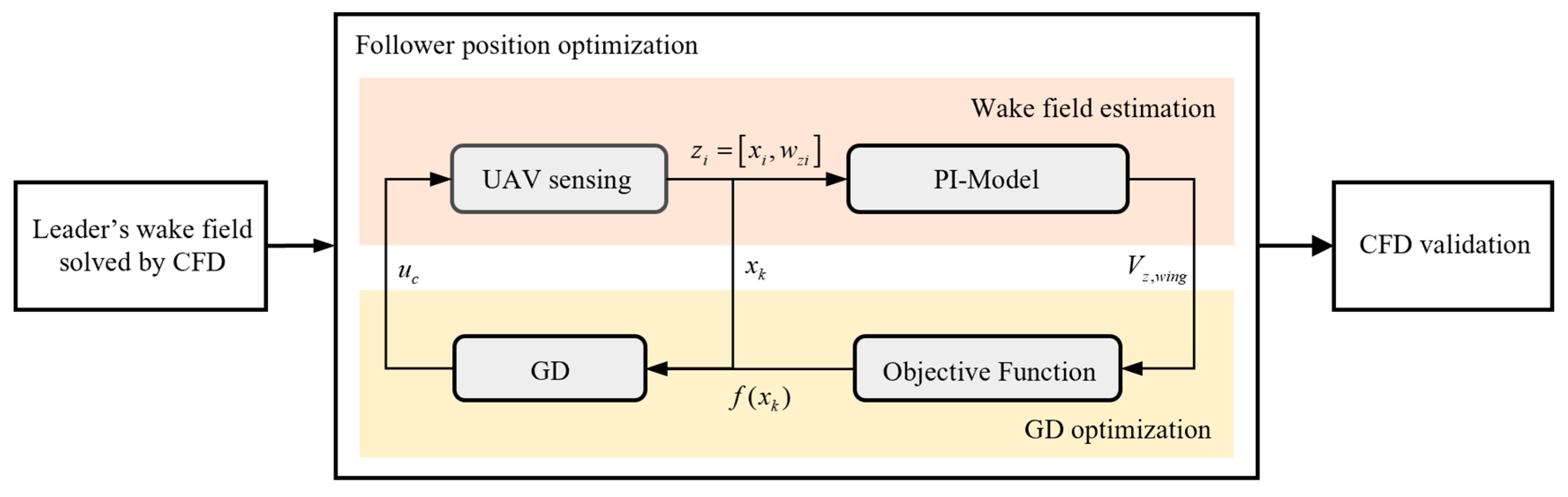
First, the CFD is used to solve the wake field of the leader aircraft and obtain the precise distribution of the induced velocity. This provides a high-fidelity wake field environment for the follower aircraft’s position optimization, simulating real-flight conditions as closely as possible.
Subsequently, formation position optimization is performed based on the GD algorithm, with the induced drag defined as the objective function—maximizing the wake benefit is equivalent to minimizing the induced drag. The follower’s position is first initialized, and under the guidance of the GD, the follower UAV uses its on-board sensing system, which includes two ADS units, to perceive the local wake velocity in real time. The IPIO algorithm is then employed to identify the PI-Model parameters, enabling estimation of the wake field distribution. The objective function and its gradient are calculated in real time, guiding the follower UAV to iteratively adjust its position toward the optimal point.
Finally, to verify whether the converged position represents the optimal relative position, CFD simulations are conducted for comparative validation. Specifically, around the convergence point of the GD, the follower aircraft is placed at several laterally offset positions (offsets of 1–20% of the wingspan relative to the converged position), and CFD calculations are performed to compute and compare the drag coefficients at these positions. By examining the drag differences, it is determined whether the converged position corresponds to the global optimum, thereby validating the effectiveness and reliability of the proposed PI-Model and formation optimization strategy.
4.2. Two-Aircraft Formation
4.2.1. Homogeneous Formation
The homogeneous two-aircraft formation (Small–Small) is analyzed first. The wake field of the leader aircraft is computed using CFD to obtain the three-dimensional induced velocity field. The vertical distribution of the induced velocity is shown in Figure 10, where the distinct wake vortex structures generated by the leading UAV, as well as their downstream development and dissipation characteristics, can be clearly observed.
The coordinate system is set with the center of gravity of the leader as the origin. The follower starts at the right rear of the leader, maintaining a relative distance. During the optimization process, guided by the GD algorithm, the follower continuously adjusts its relative position in real time. The sensor recordings during this process are shown in Figure 11, where the horizontal axis represents the number of iterations. The upper and middle subplots correspond to the angle of attack data measured by the two sensors and the estimated local upwash velocity, respectively. As the follower gradually moves toward the upwash region of the wake vortex, the measurements from the left sensor (Sensor 1) first increase to a maximum in the strongest upwash area, then decrease and stabilize as the aircraft continues to move, while the data from the right sensor (Sensor 2) gradually increase and stabilize. The bottom subplot shows the objective function, which exhibits a clear decreasing trend and eventually stabilizes around a constant value, indicating algorithmic convergence.
The flight trajectory of the follower aircraft in the leader's wake velocity field is shown as the red trajectory in Figure 12. From the trajectory curve, it can be observed that under the real-time guidance of the algorithm, the follower gradually moves toward the position of strongest upwash, with the optimization path converging to the optimal point.
CFD numerical simulations are used for validation to verify whether the position at which the algorithm converges is optimal, as shown in Figure 13. Specifically, using the converged position from the algorithm as the reference point, the follower aircraft is displaced laterally to the left and right by 1%, 2%, 5%, 10%, and 20% of the wingspan distance. The drag coefficients at each position are then calculated and compared. From the CFD results shown in Figure 14, it can be observed that the drag coefficient at the GD algorithm’s converged position is the lowest, and it is approximately 15.14% lower than the drag coefficient of the solo flight, proving that the position obtained by GD-driven UAV is indeed the optimal one.
4.2.2. Heterogeneous Formation
To verify the effectiveness of the proposed method in heterogeneous formations, this paper constructs a typical heterogeneous two-aircraft formation case with a large wingspan leader UAV (Large UAV) and a small wingspan follower UAV (Small UAV). First, the wake field of the leader UAV is computed using CFD, as shown in Figure 15.
The follower aircraft is initialized at a position relative to the leader aircraft at . During the optimization process, guided by the GD algorithm, the follower aircraft adjusts its relative position in real time. The sensor recordings during this process are shown in Figure 16, where the horizontal axis represents the number of iterations. The upper and middle subplots correspond to the angle of attack data measured by the dual sensors and the estimated local upwash velocity, respectively. As the follower aircraft gradually moves towards the wake upwash region, the measurement from Sensor 1 (left sensor) first increases to the strongest upwash point, then decreases and stabilizes as the aircraft continues to move. The measurement from Sensor 2 (right sensor) gradually increases and stabilizes. The bottom subplot shows the objective function, which exhibits a clear decreasing trend and eventually stabilizes around a constant value, indicating that the algorithm has converged. Unlike the homogeneous formation, in the heterogeneous formation, the leader aircraft is larger, resulting in a stronger induced wake field, which provides the follower aircraft with stronger upwash and drag reduction benefits.
The flight trajectory during the position optimization process is recorded, as shown in Figure 17, where the red trajectory represents the movement of the follower aircraft during the real-time optimization process. The follower aircraft eventually converges to position .
To confirm that the position to which the GD algorithm converges is indeed the optimal one, CFD simulations are used for validation, as shown in Figure 18. The CFD results are presented in Figure 19, where it can be seen that the drag coefficient at the converged position is the lowest, and the drag reduction efficiency is the highest, thereby validating that the converged position is the optimal one. Furthermore, compared to solo flight, the follower aircraft experiences a drag reduction of approximately 24.48%, demonstrating that the large wingspan leader aircraft provides significantly stronger aerodynamic benefits to the follower.
4.3. Result Discussion
From the simulation results of two typical scenarios, homogeneous two-aircraft formation and heterogeneous two-aircraft formation, the following conclusions can be drawn:
- Real-time optimization is effective: In the above scenarios, the PI-Model based on onboard sensor wake identification, and the GD optimization algorithm both achieve stable convergence. This ensures that the follower aircraft quickly finds the optimal formation position, meeting the real-time formation control requirements and demonstrating potential for practical application;
- Position accuracy validation: CFD validation shows that the relative positions obtained using the proposed method result in drag reduction efficiencies of 15% and 25% under different conditions, respectively, compared to solo flight. The lateral steady-state error in position optimization is controlled within 1% of the wingspan, proving the algorithm's satisfactory accuracy and effectiveness.
5. Conclusions
This paper focuses on aerodynamic energy optimization for fixed-wing UAV formation flight in complex scenarios, aiming to address the limitations of traditional aerodynamic simulation optimization in terms of efficiency. A bio-inspired approach is proposed, utilizing the PI-Model based on onboard sensor. The model's accuracy and its effectiveness in estimating formation aerodynamic effects are validated through comparison with CFD results. Furthermore, to verify the effectiveness and accuracy of the proposed method, a series of typical formation scenario simulations are designed and conducted, covering both homogeneous and heterogeneous two-aircraft configurations. By analyzing the convergence performance and optimization effects, the performance of the proposed method in formation position optimization is evaluated. The paper can be summarized as follows:
- The wake vortex estimation method, PI-Model, proposed in this paper minimizes the wake-induced velocity residuals using the IPIO algorithm, enabling accurate identification of key wake vortex parameters and significantly enhancing the accuracy and versatility of wake velocity estimation. Compared to CFD results, the PI-Model improves the precision of wake field velocity sensing and formation aerodynamic effect estimation. Additionally, the PI-Model samples the real-time wake field using a multi-sensor system with two ADS units, ensuring high estimation performance while significantly reducing hardware and computational costs. This makes the method suitable for deployment on low-cost UAV platforms and demonstrates its potential for application in multi-UAV complex formation scenarios;
- PI-Model enables online estimation of parameters through real-time individual sensor feedback, providing "wake tracking" capability. Compared to other formation aerodynamic modeling methods, this approach allows for dynamic updates of wake changes, improving the accuracy of wake vortex estimation. In formation scenarios, this results in the continuous identification of the optimal position, thereby enhancing the aerodynamic benefits of the formation;
- The effectiveness of the wake vortex estimation and formation optimization methods is validated through the construction of formation simulation. In various scenarios presented in this paper, the formation positions achieved stable convergence. Compared to solo flight, the drag reduction efficiency of the follower aircraft in the formation flight reached 15% and 25% under different conditions. CFD validation confirmed that the steady-state error at the converged position was controlled within 1% of the wingspan, demonstrating the satisfactory accuracy and effectiveness of the proposed method.
In summary, the PI-Model based on onboard sensor and online identification proposed in this paper demonstrates strong performance in terms of accuracy, efficiency, and versatility. This method provides a feasible and low-cost approach for achieving fast, adaptive, and energy-efficient formations, with potential for scaling to larger heterogeneous mixed UAV fleets for collaborative flight missions. It holds significant theoretical importance and engineering value for improving the airspace utilization, energy efficiency, and mission coordination of future UAV swarms. To further enhance this method and increase its practicality, in-depth research is needed to address the complex environments that may be encountered in real-world applications.
Future research will focus on the following key areas: First, the proposed method will be validated through actual flight tests, considering the tracking performance of the flight controller. Second, the impact of meteorological disturbances in real flight environments and the effect of real sensor noise on the wake model estimation accuracy and optimization algorithm will be investigated.
Author Contributions
Conceptualization, T.G. and J.F.; methodology, T.G., B.C., L.T. and J.F.; software, T.G.; validation, T.G., Y.Y. and J.F.; formal analysis, T.G.; investigation, T.G.; resources, T.G.; data curation, T.G.; writing—original draft preparation, T.G.; writing—review and editing, J.F.; visualization, T.G.; supervision, T.M.; project administration, T.M.; funding acquisition, T.M. All authors have read and agreed to the published version of the manuscript.
Funding
This research was funded by Beijing Natural Science Foundation (No.QY24131) , the Fundamental Research Funds for the Central Universities (No.501QYJC2024129001), Aeronautical Science Foundation of China (ASFC)(No.2024Z006051002) and the Taihu Innovation Fund for Future Technology (No.1311402).
Data Availability Statement
The datasets generated during and/or analyzed during the current study are available from the corresponding author on reasonable request.
Conflicts of Interest
The authors declare no conflicts of interest.
References
- Lissaman, P.B.S.; Shollenberger, C.A. Formation Flight of Birds. Science 1970, 168, 1003–1005.
- Weimerskirch, H.; Martin, J.; Clerquin, Y.; Alexandre, P.; Jiraskova, S. Energy Saving in Flight Formation. Nature 2001, 413, 697–698. [CrossRef]
- Portugal, S.J.; Hubel, T.Y.; Fritz, J.; Heese, S.; Trobe, D.; Voelkl, B.; Hailes, S.; Wilson, A.M.; Usherwood, J.R. Upwash Exploitation and Downwash Avoidance by Flap Phasing in Ibis Formation Flight. Nature 2014, 505, 399–402. [CrossRef]
- Ray, R.; Cobleigh, B.; Vachon, M.; St. John, C. Flight Test Techniques Used to Evaluate Performance Benefits During Formation Flight. In Proceedings of the AIAA Atmospheric Flight Mechanics Conference and Exhibit; American Institute of Aeronautics and Astronautics: Monterey, California, August 5 2002.
- Kent, T.E.; Richards, A.G. Analytic Approach to Optimal Routing for Commercial Formation Flight. Journal of Guidance, Control, and Dynamics 2015, 38, 1872–1884. [CrossRef]
- Bangash, Z.A.; Sanchez, R.P.; Ahmed, A.; Khan, M.J. Aerodynamics of Formation Flight. Journal of Aircraft 2006, 43, 907–912. [CrossRef]
- Hanson, C.E.; Pahle, J.; Reynolds, J.R.; Andrade, S.; Nelson, B. Experimental Measurements of Fuel Savings During Aircraft Wake Surfing. In Proceedings of the 2018 Atmospheric Flight Mechanics Conference; American Institute of Aeronautics and Astronautics: Atlanta, Georgia, June 25 2018.
- Zhang, Q.; Liu, H.H.T. Robust Nonlinear Close Formation Control of Multiple Fixed-Wing Aircraft. Journal of Guidance, Control, and Dynamics 2021, 44, 572–586. [CrossRef]
- Wang, R.; Zhou, Z.; Lungu, M.; Li, L. PSD INDI and Wake Gradient Based Control of High Aspect Ratio UAVs’ Close Formation Flight. Aerospace Science and Technology 2025, 162, 110198. [CrossRef]
- Sheng, H.; Zhang, J.; Yan, Z.; Yin, B.; Liu, S.; Bai, T.; Wang, D. New Multi-UAV Formation Keeping Method Based on Improved Artificial Potential Field. Chinese Journal of Aeronautics 2023, 36, 249–270. [CrossRef]
- Tao, Y.; Xiong, N.; Wang, X.; Lin, J.; Liu, Z.; Ma, S.; Wu, J. Experimental and Computational Investigation of Hybrid Formation Flight for Aerodynamic Gain at Transonic Speed. Chinese Journal of Aeronautics 2021, 34, 32–43. [CrossRef]
- Yang, M.; Guan, X.; Shi, M.; Li, B.; Wei, C.; Yiu, K.-F.C. Distributed Model Predictive Formation Control for UAVs and Cooperative Capability Evaluation of Swarm. Drones 2025, 9, 366. [CrossRef]
- Martinez-Ponce, J.; Herkenhoff, B.; Aboelezz, A.; Urban, C.; Armanini, S.; Raphael, E.; Hassanalian, M. Studies on V-Formation and Echelon Flight Utilizing Flapping-Wing Drones. Drones 2024, 8, 395. [CrossRef]
- Yuan, G.; Duan, H. Robust Control for UAV Close Formation Using LADRC via Sine-Powered Pigeon-Inspired Optimization. Drones 2023, 7, 238. [CrossRef]
- Zhu, H.; Wu, S. Leader–Follower Formation Reconfiguration Control for Fixed-Wing UAVs Using Multiplayer Stackelberg–Nash Game. Drones 2025, 9, 439. [CrossRef]
- Ma, B.; Liu, Z.; Jiang, F.; Zhao, W.; Dang, Q.; Wang, X.; Zhang, J.; Wang, L. Reinforcement Learning Based UAV Formation Control in GPS-Denied Environment. Chinese Journal of Aeronautics 2023, 36, 281–296. [CrossRef]
- Cho, J.; Lee, B.J.; Misaka, T.; Yee, K. Study on Decay Characteristics of Vertical Four-Vortex System for Increasing Airport Capacity. Aerospace Science and Technology 2020, 105, 106017. [CrossRef]
- Kless, J.E.; Aftosmis, M.J.; Ning, S.A.; Nemec, M. Inviscid Analysis of Extended-Formation Flight. AIAA Journal 2013, 51, 1703–1715. [CrossRef]
- Qiao, N.; Ma, T.; Wang, X.; Wang, J.; Fu, J.; Xue, P. An Approach for Formation Design and Flight Performance Prediction Based on Aerodynamic Formation Unit: Energy-Saving Considerations. Chinese Journal of Aeronautics 2024, 37, 77–91. [CrossRef]
- Al-Mahadin, A.; Almajali, M. Simplified Mathematical Modelling of Wing Tip Vortices. In Proceedings of the 2019 Advances in Science and Engineering Technology International Conferences (ASET); IEEE: Dubai, United Arab Emirates, March 2019; pp. 1–6.
- Dogan, A.; Venkataramanan, S.; Blake, W. Modeling of Aerodynamic Coupling Between Aircraft in Close Proximity. Journal of Aircraft 2005, 42, 941–955. [CrossRef]
- Brodecki, M.; Subbarao, K. Autonomous Formation Flight Control System Using In-Flight Sweet-Spot Estimation. Journal of Guidance, Control, and Dynamics 2015, 38, 1083–1096. [CrossRef]
- Melin, T. A Vortex Lattice MATLAB Implementation for Linear Aerodynamic Wing Applications., Royal Institute of Technology: Sweden, 2000.
- Peristy, L.H.; Perez, R.E.; Jansen, P.W. Wake Modelling with Embedded Lateral and Directional Stability Sensitivity Analysis for Aerial Refuelling or Formation Flight. In Proceedings of the AIAA Scitech 2019 Forum; American Institute of Aeronautics and Astronautics: San Diego, California, January 7 2019.
- Zhang, Q.; Liu, H.H.T. Aerodynamics Modeling and Analysis of Close Formation Flight. Journal of Aircraft 2017, 54, 2192–2204. [CrossRef]
- Yuan, G.; Xia, J.; Duan, H. A Continuous Modeling Method via Improved Pigeon-Inspired Optimization for Wake Vortices in UAVs Close Formation Flight. Aerospace Science and Technology 2022, 120, 107259. [CrossRef]
- Unterstrasser, S.; Stephan, A. Far Field Wake Vortex Evolution of Two Aircraft Formation Flight and Implications on Young Contrails. Aeronaut. j. 2020, 124, 667–702. [CrossRef]
- Edstrand, A.M.; Davis, T.B.; Schmid, P.J.; Taira, K.; Cattafesta, L.N. On the Mechanism of Trailing Vortex Wandering. J. Fluid Mech. 2016, 801. [CrossRef]
- Lin, M.; Huang, W.; Zhang, Z.; Xu, C.; Cui, G. Numerical Study of Aircraft Wake Vortex Evolution near Ground in Stable Atmospheric Boundary Layer. Chinese Journal of Aeronautics 2017, 30, 1866–1876. [CrossRef]
- Pan, W.; Deng, L.; Leng, Y.; Li, F. Wake Vortex Safety Assessment during Cruise Using a Regional Medium-Short-Range Turbofan Aircraft as an Example. Chinese Journal of Aeronautics 2025, 38, 103283. [CrossRef]
- Michel, D.T.; Dolfi-Bouteyre, A.; Goular, D.; Augère, B.; Planchat, C.; Fleury, D.; Lombard, L.; Valla, M.; Besson, C. Onboard Wake Vortex Localization with a Coherent 1.5 Μm Doppler LIDAR for Aircraft in Formation Flight Configuration. Opt. Express 2020, 28, 14374. [CrossRef]
- Wei, Z.; Lu, T.; Gu, R.; Liu, F. DBN-GABP Model for Estimation of Aircraft Wake Vortex Parameters Using Lidar Data. Chinese Journal of Aeronautics 2024, 37, 347–368. [CrossRef]
- Rodenhiser, R.J.; Durgin, W.W.; Johari, H. Ultrasonic Method for Aircraft Wake Vortex Detection. Journal of Aircraft 2007, 44, 726–732. [CrossRef]
- Hallock, J.N.; Holzäpfel, F. A Review of Recent Wake Vortex Research for Increasing Airport Capacity. Progress in Aerospace Sciences 2018, 98, 27–36. [CrossRef]
- Steen, M.; Hecker, P. Investigating the Potential Future Usage of Combined Airborne Wake Vortex Prediction Models and Measurement Sensors. In Proceedings of the 2018 Atmospheric and Space Environments Conference; American Institute of Aeronautics and Astronautics: Atlanta, Georgia, June 25 2018.
- Hemati, M.S.; Eldredge, J.D.; Speyer, J.L. Wake Sensing for Aircraft Formation Flight. Journal of Guidance, Control, and Dynamics 2014, 37, 513–524. [CrossRef]
- DeVries, L.; Paley, D.A. Wake Sensing and Estimation for Control of Autonomous Aircraft in Formation Flight. Journal of Guidance, Control, and Dynamics 2016, 39, 32–41. [CrossRef]
- GuangSong, Y.; HaiBin, D. Extremum Seeking Control for UAV Close Formation FLight via Improved Pigeon-Inspired Optimization. 2024, 67.
Figure 1.
Flight platform and sensor configuration.
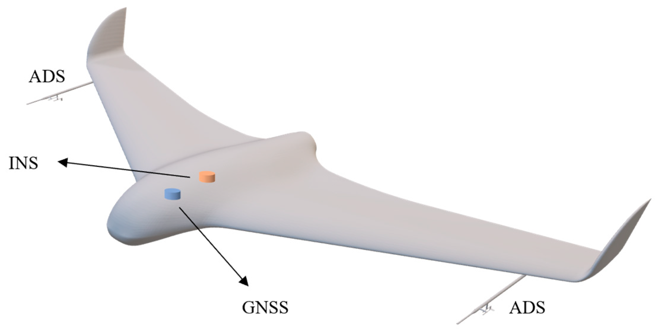
Figure 2.
The Unscented Kalman Filter Algorithm.
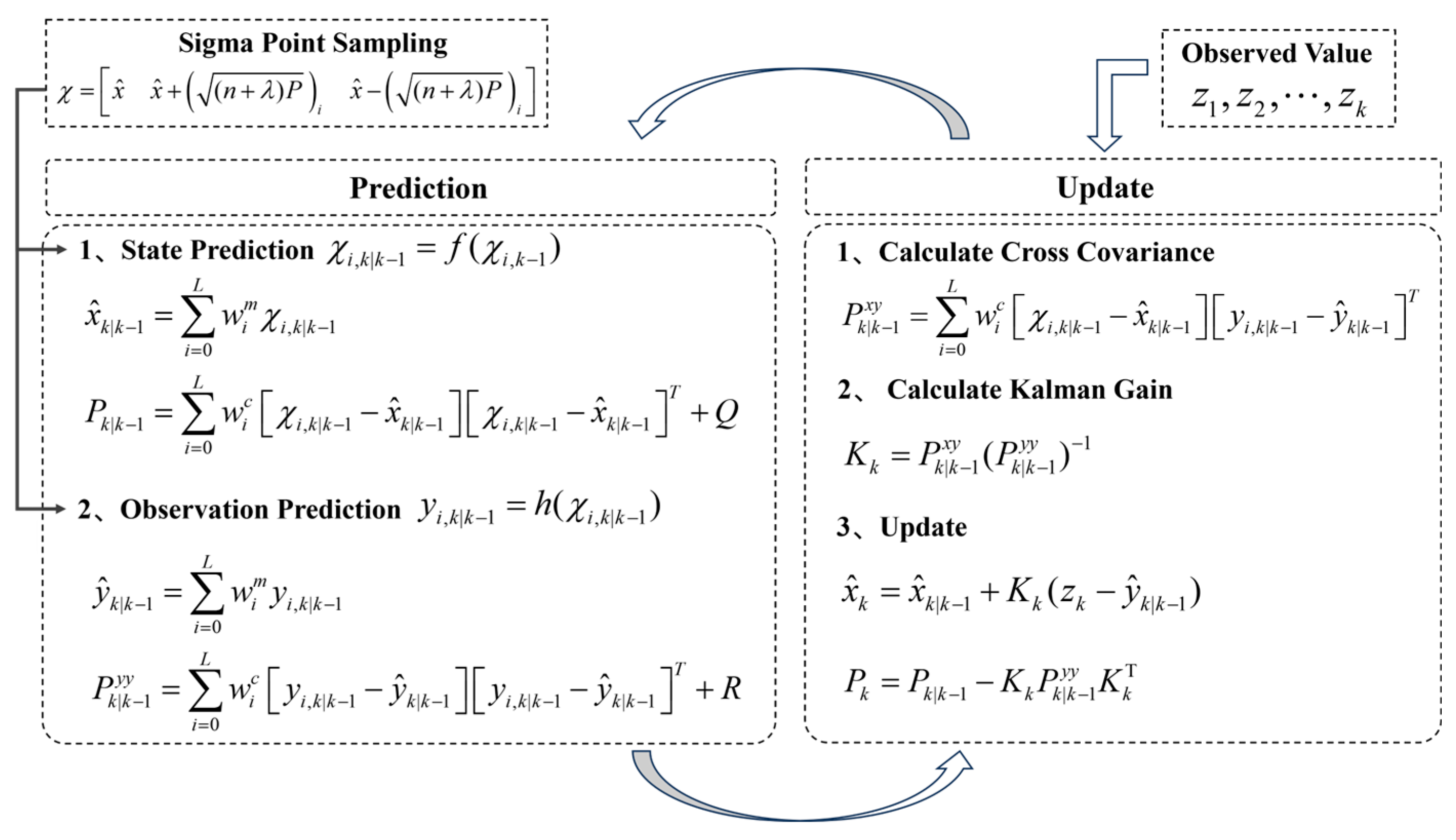
Figure 3.
Flowchart of PI-Model parameter identification based on IPIO.
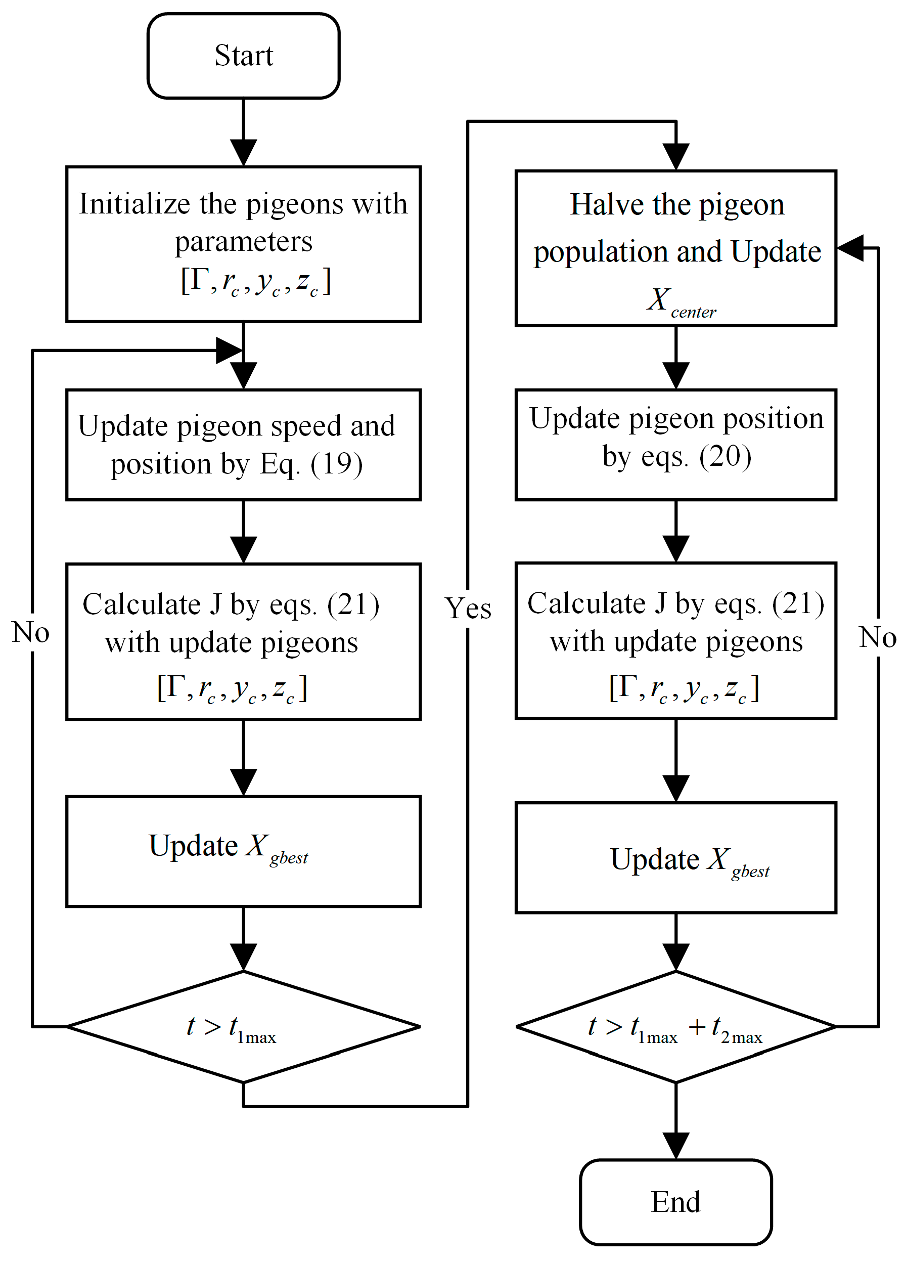
Figure 4.
Vertical induced velocity variations with lateral spacing.
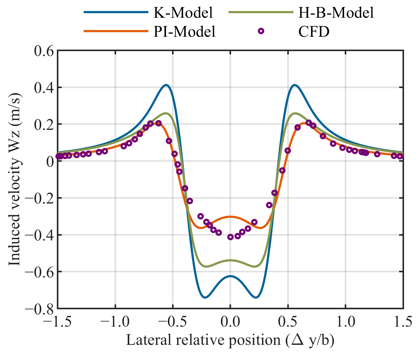
Figure 5.
lateral induced velocity variations with lateral spacing.
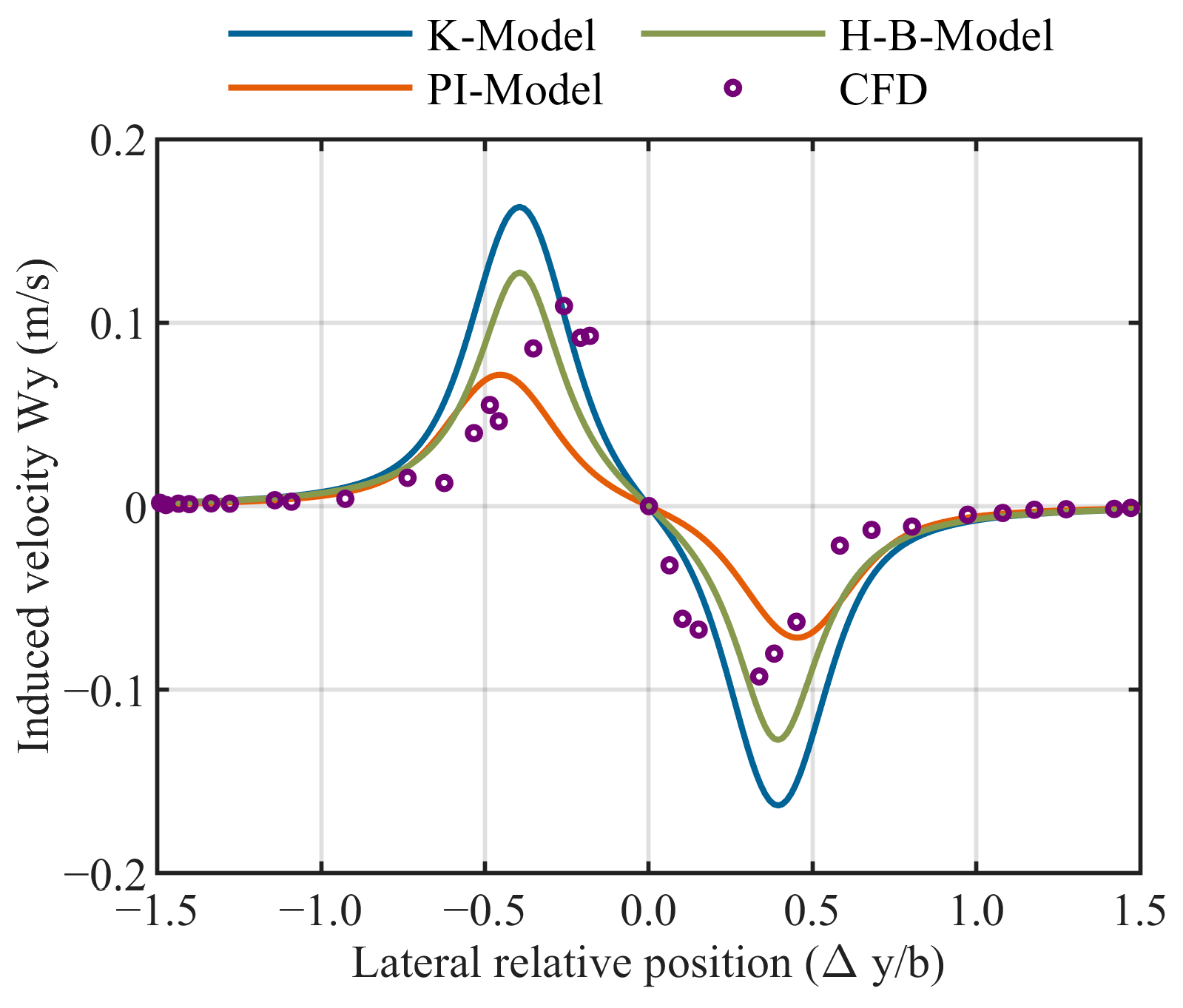
Figure 6.
Induced lift coefficient variations with lateral spacing.
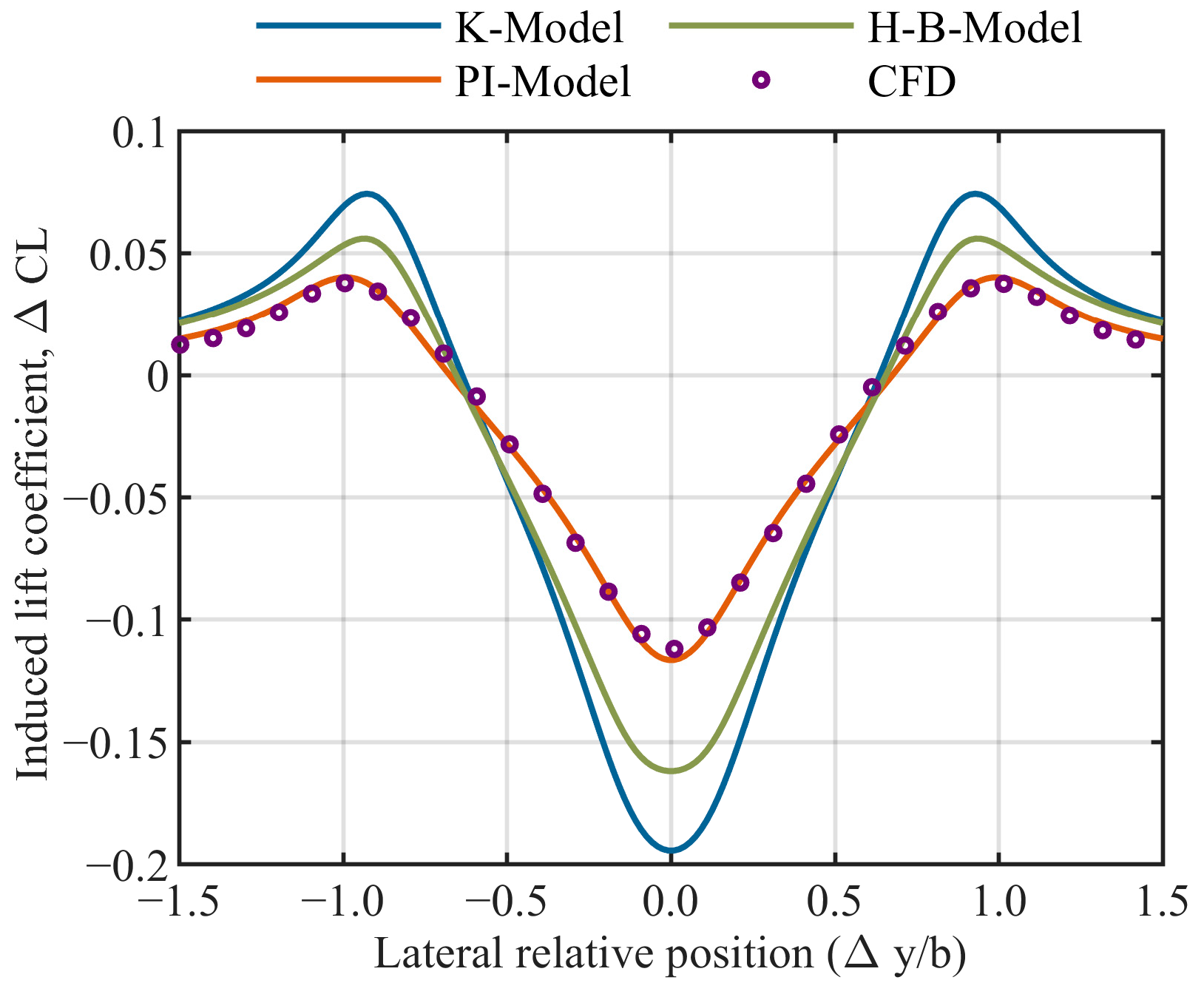
Figure 7.
Induced drag coefficient variations with lateral spacing.
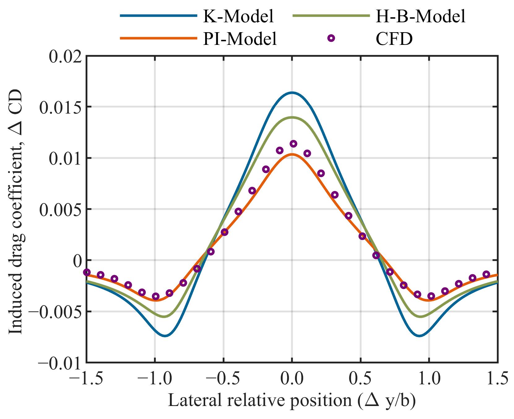
Figure 8.
Induced rolling moment coefficient variations with lateral spacing .
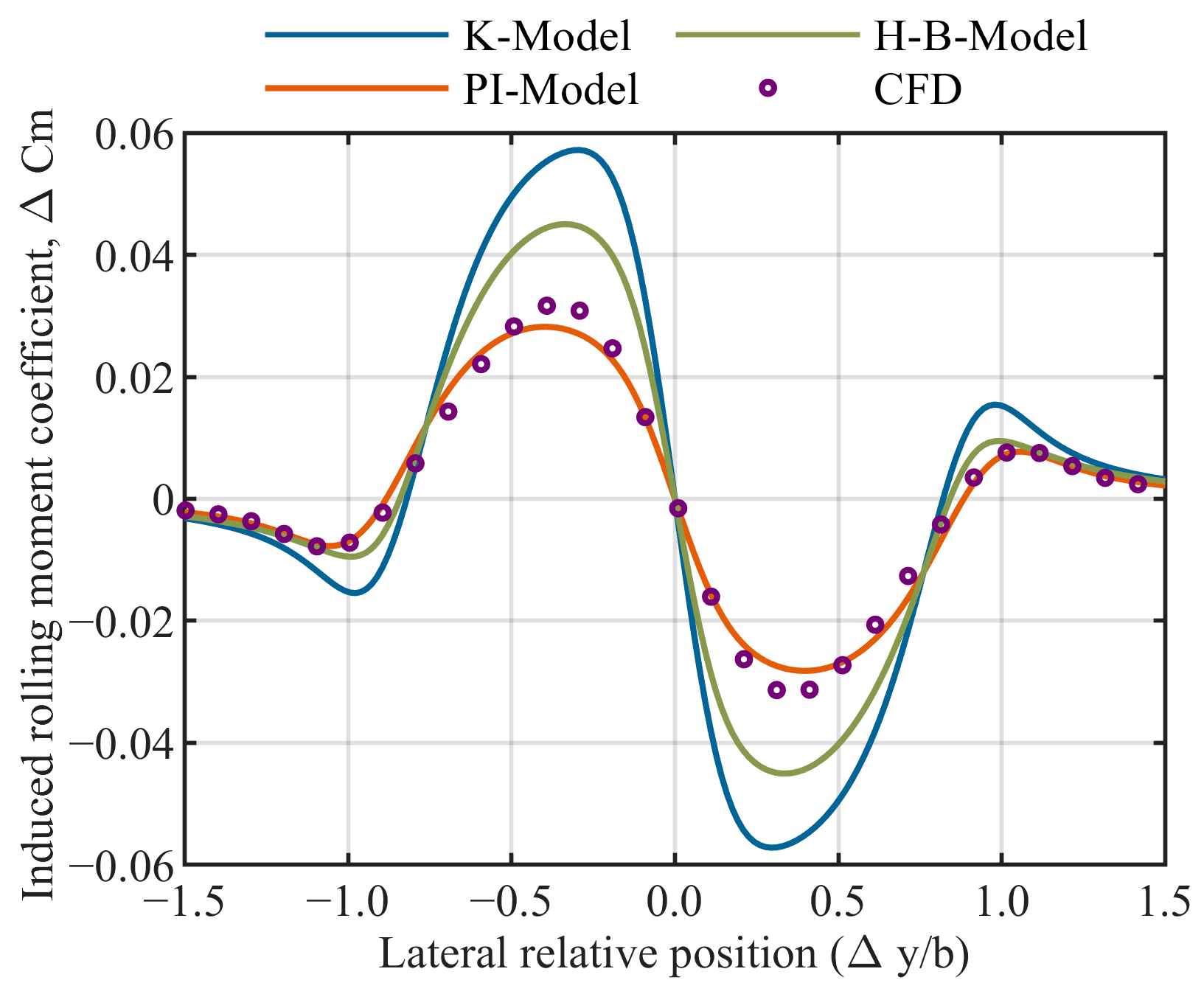
Figure 10.
Distribution of the z-components of the velocity behind the leader.
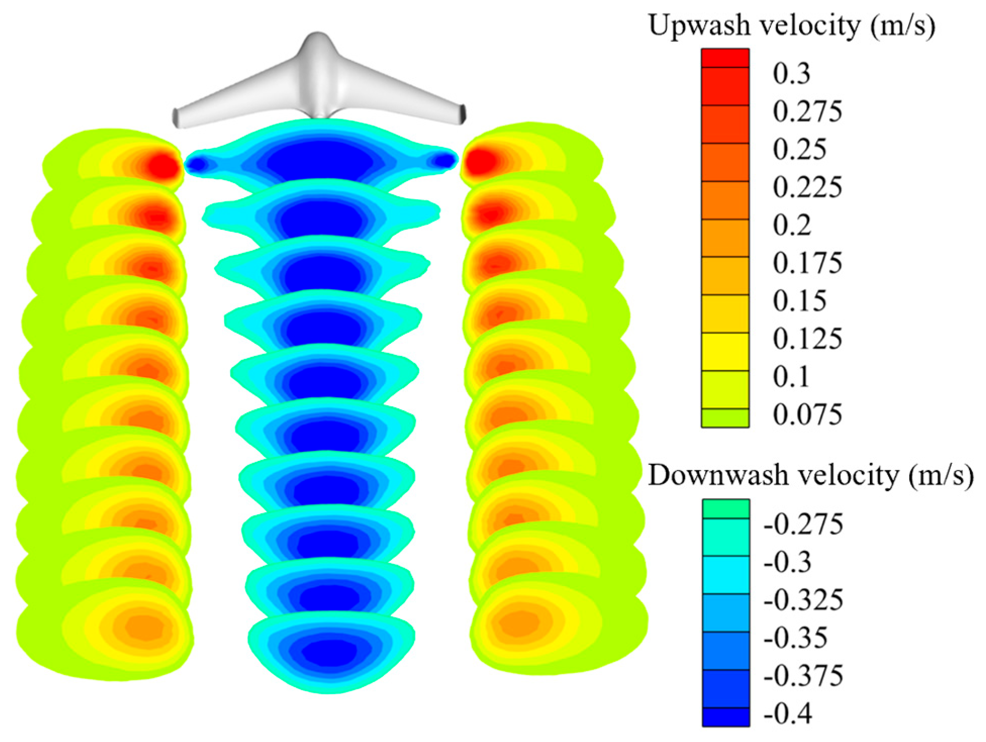
Figure 11.
Sensor data and objective function of Follower.
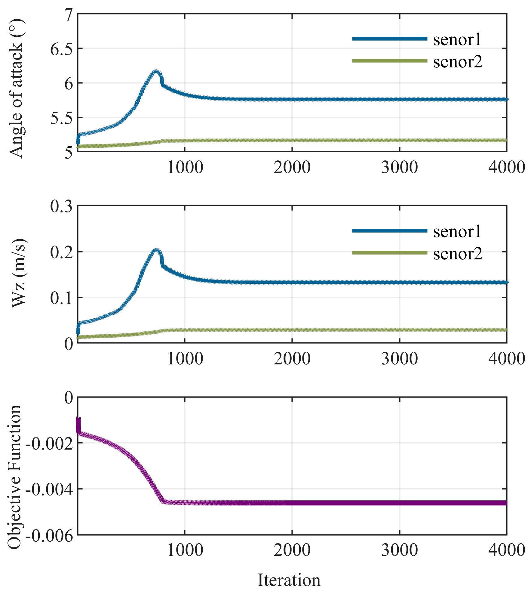
Figure 12.
Flight path of the Follower during GD.
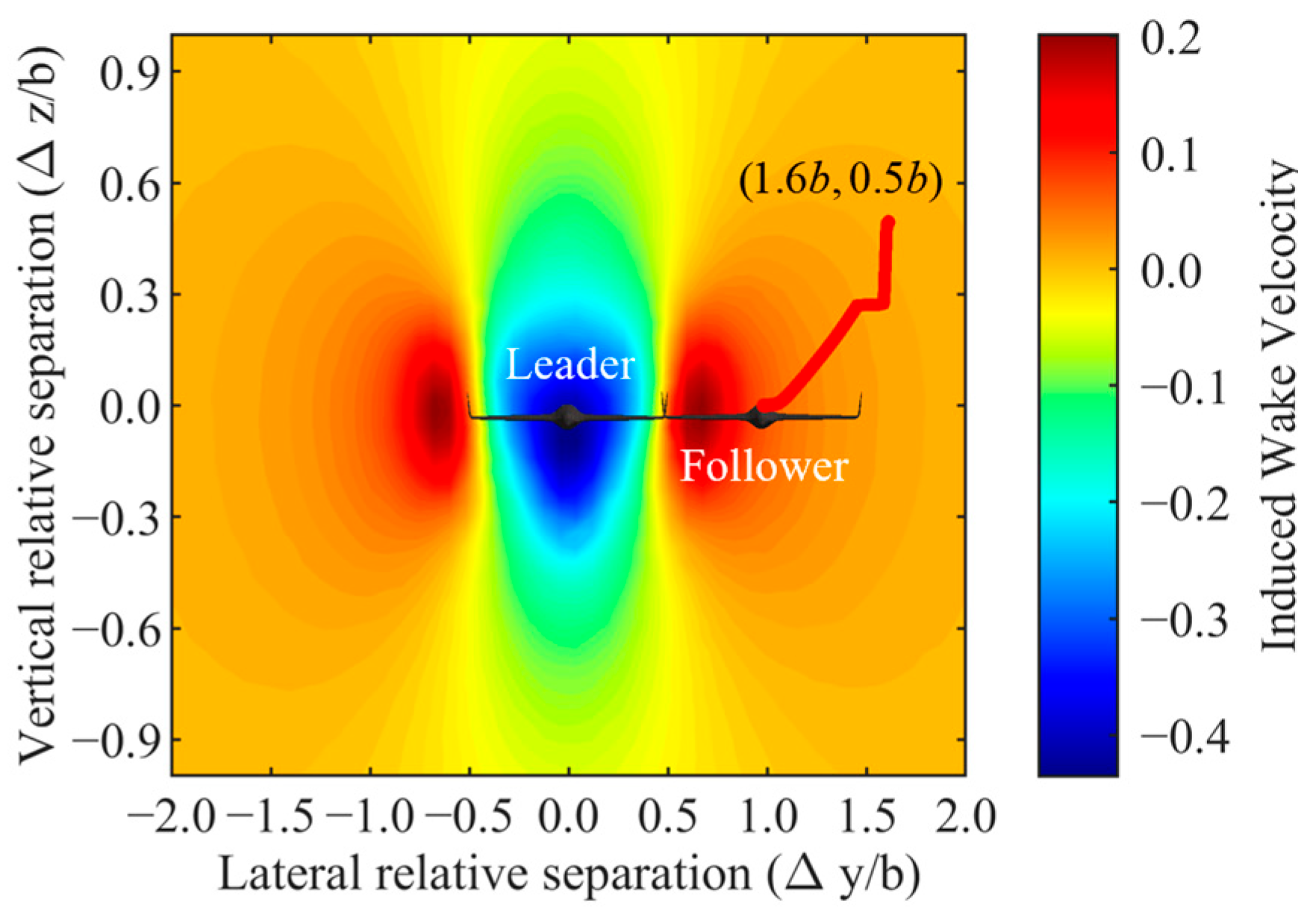
Figure 13.
Vortex strength contour plot for two aircraft.
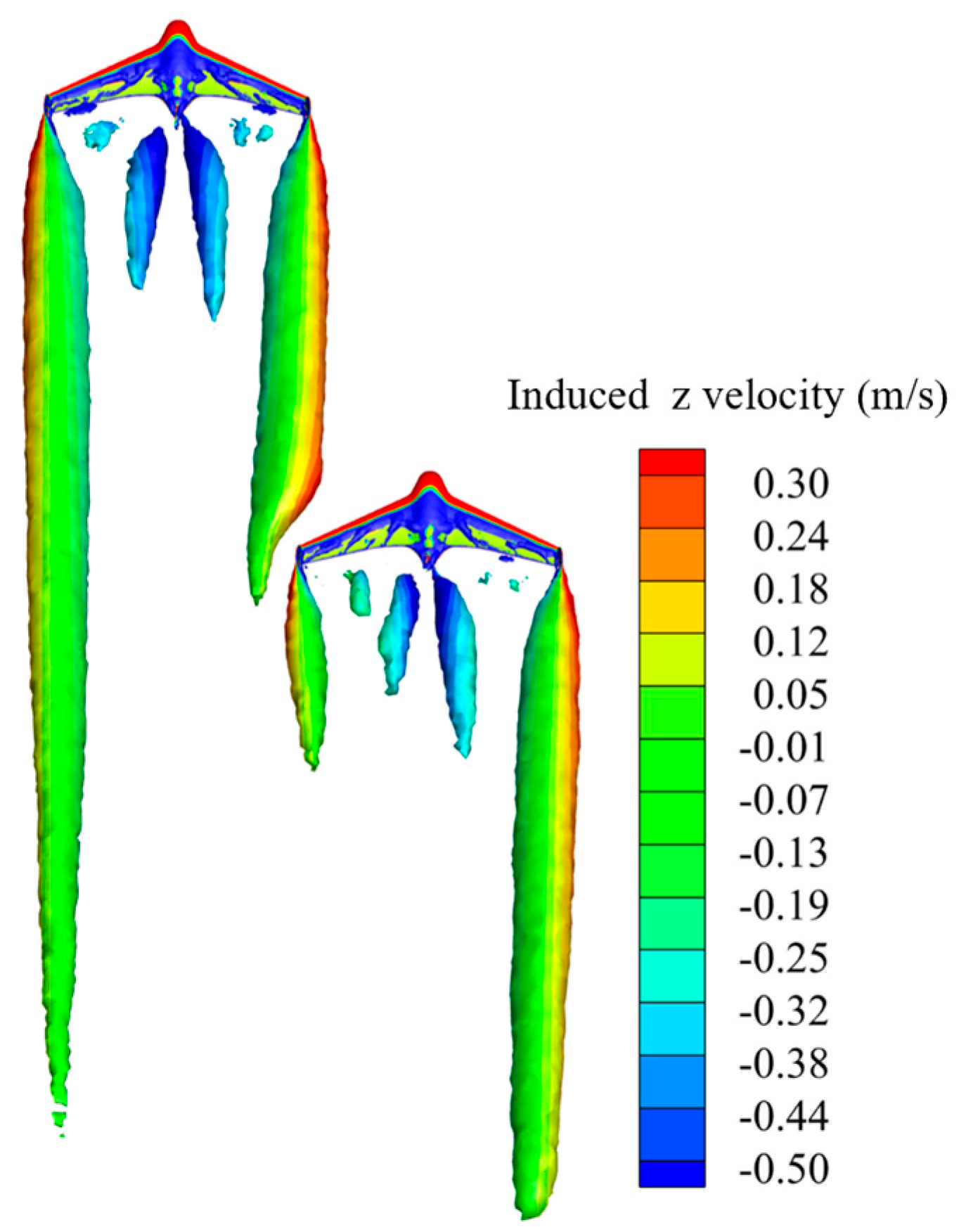
Figure 14.
Drag coefficient of the Follower1 at various lateral positions.
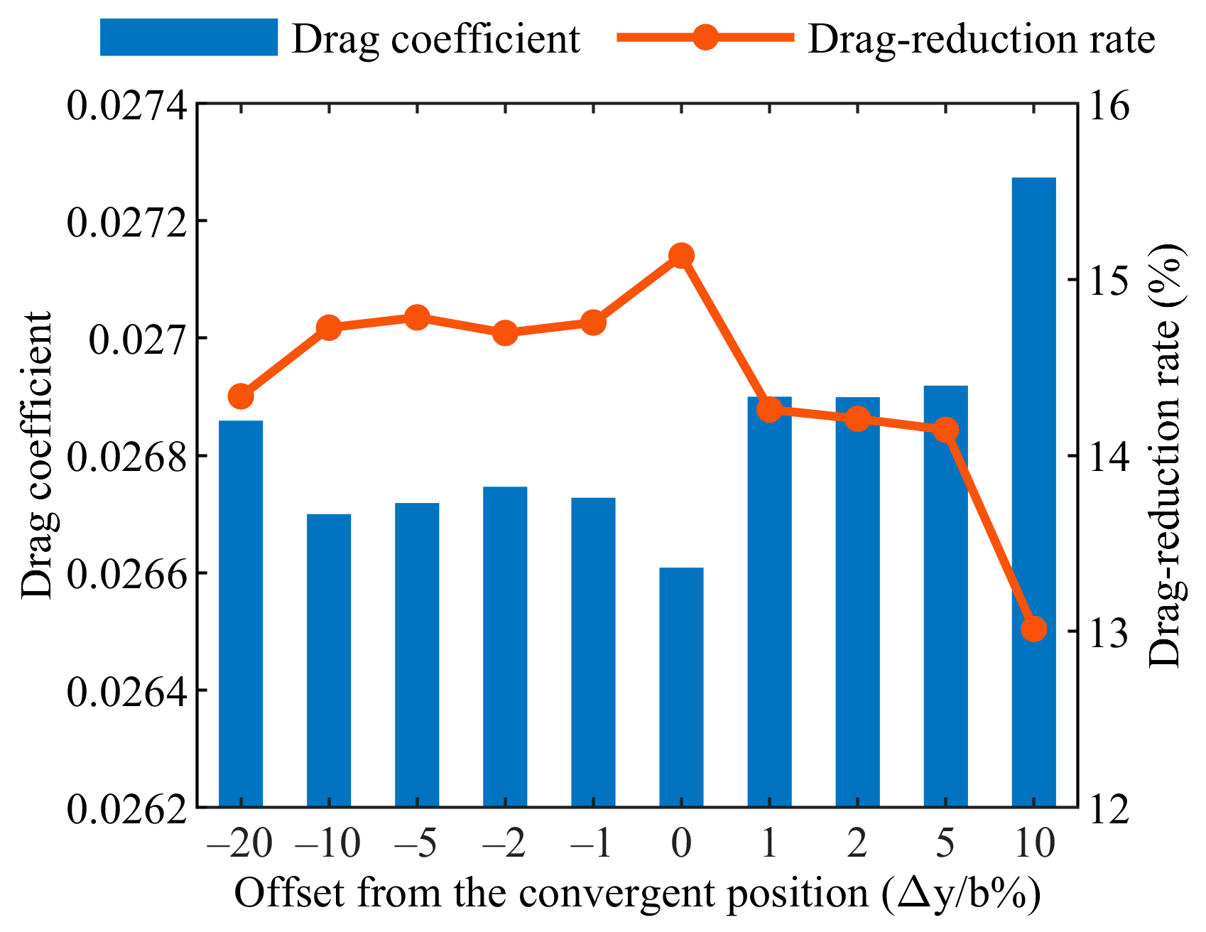
Figure 15.
Distribution of the z-components of the velocity behind the leader.
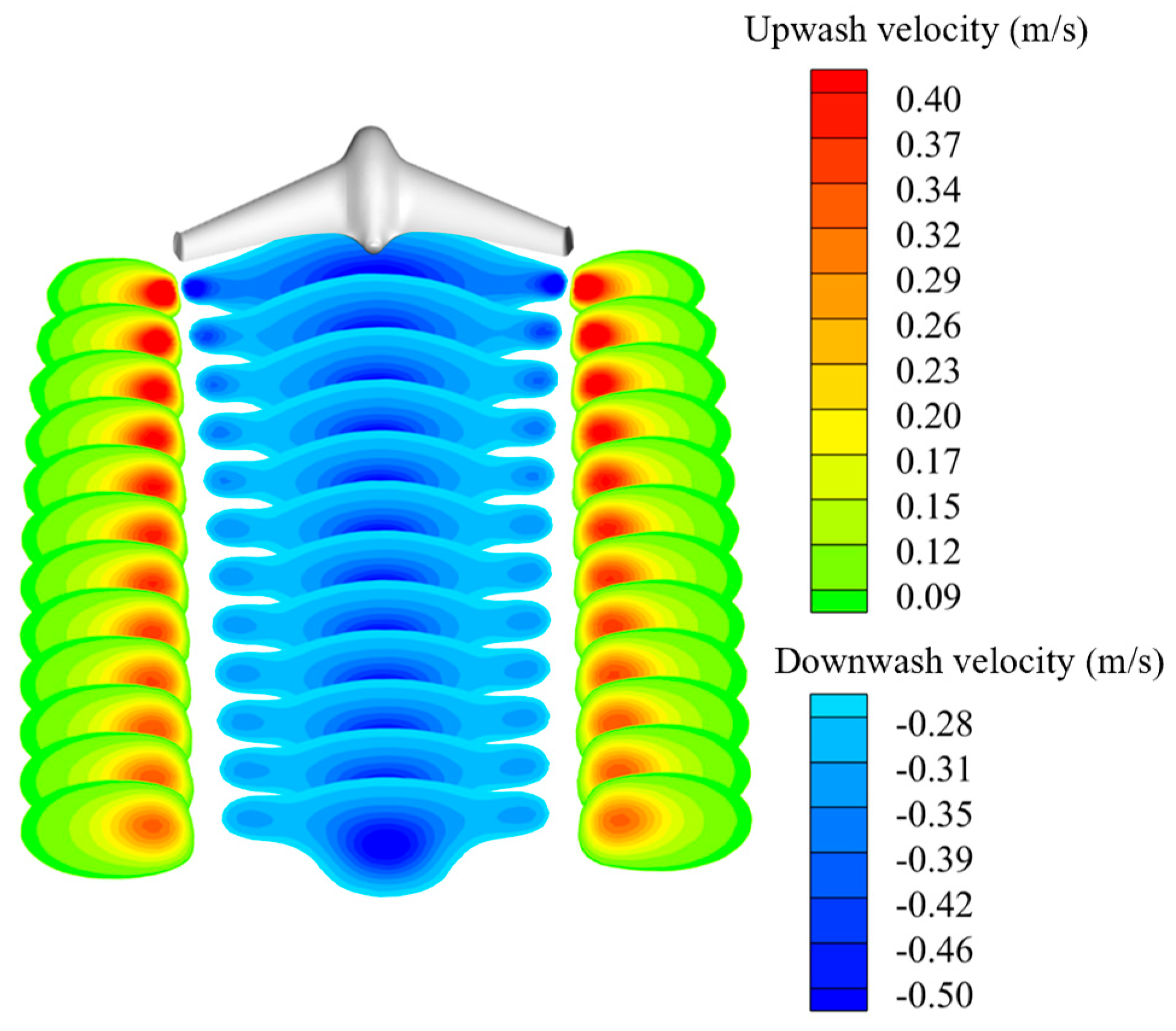
Figure 16.
Sensor data and objective function of Follower.
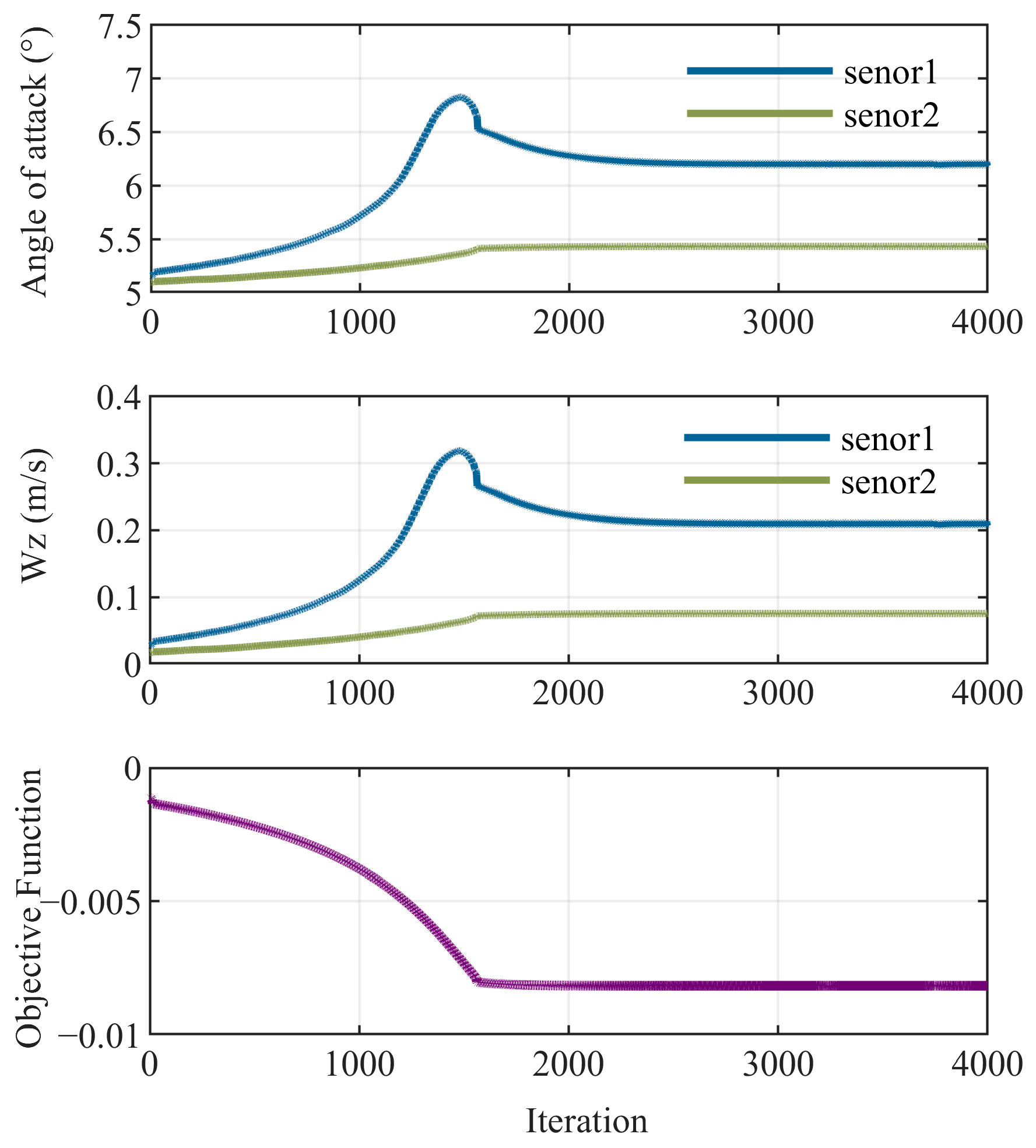
Figure 17.
Flight path of the Follower during GD.
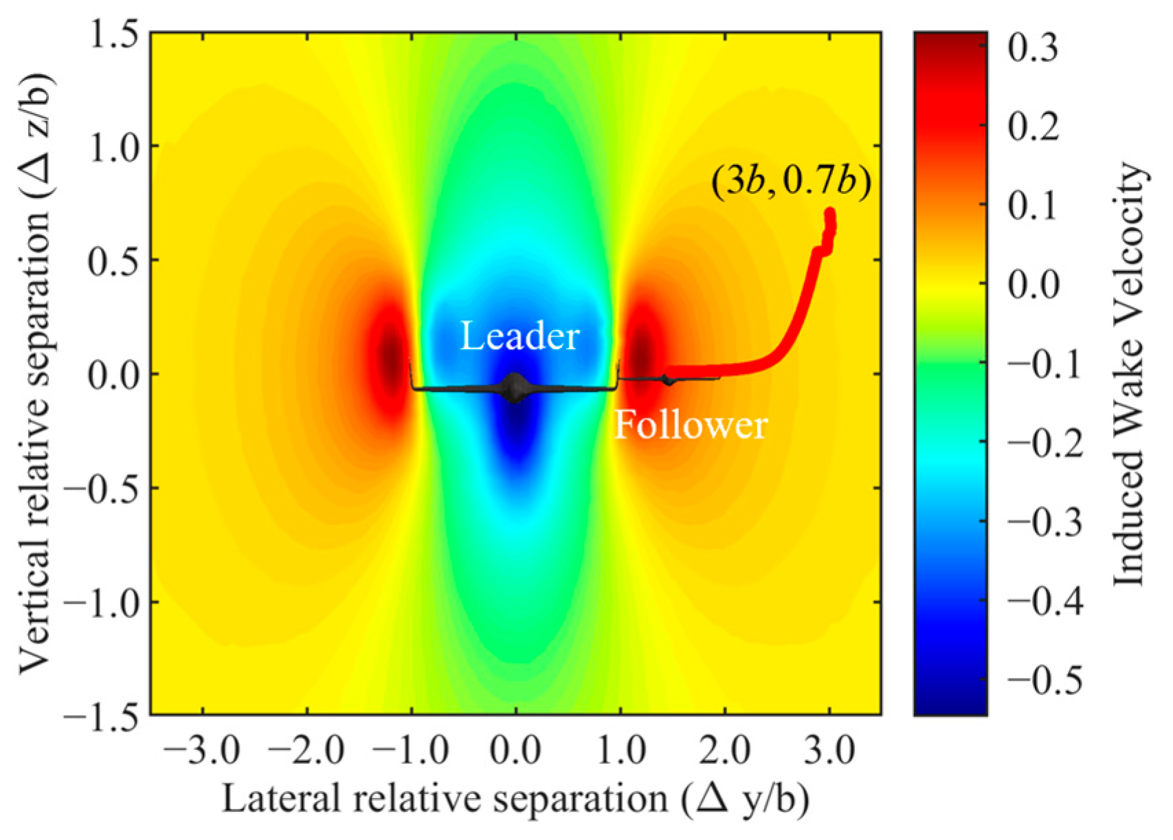
Figure 18.
Vortex strength contour plot for two aircraft.
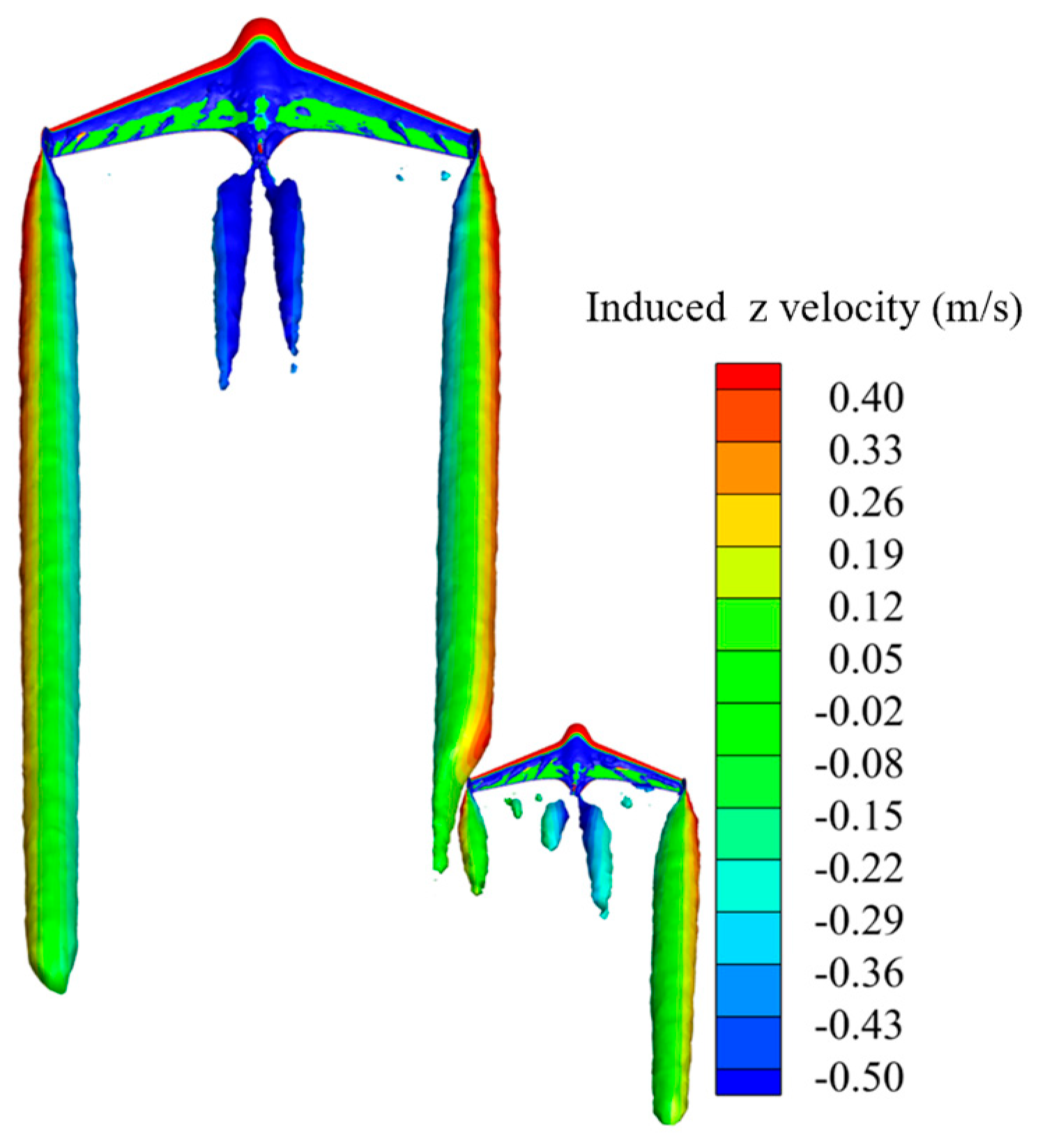
Figure 19.
Drag coefficient of the Follower at various lateral positions.
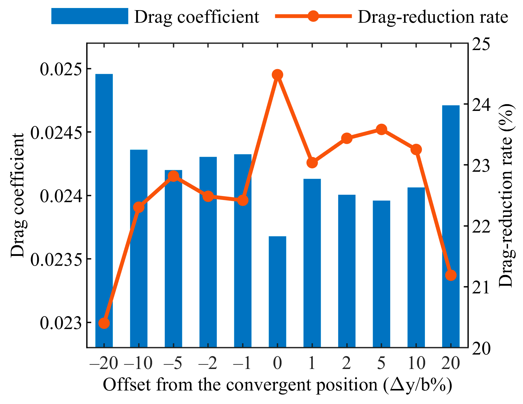

Table 1.
Table 1. Aircraft parameters.
| Parameters | UAV |
|---|---|
| span/m | 2.1039 |
| chord/m | 0.4080 |
| mass/kg | 1.8404 |
| wing area/m2 | 0.7456 |
Table 2.
Parameters of Large UAV and Small UAV.
| Parameters | LargeUAV | SmallUAV |
|---|---|---|
| span/m | 4.2078 | 2.1039 |
| chord/m | 0.8160 | 0.4080 |
| mass/kg | 7.3616 | 1.8404 |
| wing area/m2 | 2.9824 | 0.7456 |
Disclaimer/Publisher’s Note: The statements, opinions and data contained in all publications are solely those of the individual author(s) and contributor(s) and not of MDPI and/or the editor(s). MDPI and/or the editor(s) disclaim responsibility for any injury to people or property resulting from any ideas, methods, instructions or products referred to in the content. |
© 2025 by the authors. Licensee MDPI, Basel, Switzerland. This article is an open access article distributed under the terms and conditions of the Creative Commons Attribution (CC BY) license (http://creativecommons.org/licenses/by/4.0/).
Copyright: This open access article is published under a Creative Commons CC BY 4.0 license, which permit the free download, distribution, and reuse, provided that the author and preprint are cited in any reuse.


