
Submitted:
10 October 2025
Posted:
14 October 2025
You are already at the latest version
Abstract
This research introduces a comprehensive parametric copula regression framework, meticulously designed to model the joint behavior of two response variables, specifically conditioned on a chosen predictor variable. The innovative methodology effectively synthesizes parametric regression techniques for the marginal distributions with a copula function, which adeptly captures the intricate dependence structure between the response variables. Leveraging Sklar’s theorem, the formulation of the joint conditional density is achieved by expressing it as the product of the marginal densities and a copula density. Notably, the parameter of the copula is allowed to vary as a function of the covariate, enhancing the model's flexibility and adaptability. A Gumbel copula is utilized, which is particularly adept at modeling upper-tail dependence, and its parameter is intricately linked to the predictor through a smooth parametric function, ensuring a nuanced representation of relationships. For parameter estimation, the study employs the Inference Functions for Margins (IFM) method, which facilitates efficient and accurate estimation of model parameters. Additionally, a range of diagnostic tools based on the analysis of residuals are utilized to validate the adequacy of the model, ensuring that the fit is not only statistically sound but also meaningful in practical applications. The findings of this study reveal a significant trend: the dependence between the response variables tends to diminish as the predictor variable increases. This observation highlights the critical need to address associations that depend on covariates, a factor often overlooked in traditional analyses. Overall, this proposed framework stands out as a versatile and interpretable tool for analyzing complex multivariate relationships. Its potential for application spans various fields, making it a valuable resource in both academic research and professional practice. The framework offers possibilities for deeper insights into data that involves multiple interconnected response variables, reinforcing its relevance across diverse analytical contexts.
Keywords:
copula
; parametric quantile regression
; median based unit rayleigh
1. Introduction
In the realm of multivariate regression analysis, have you ever found yourself navigating the complex landscape where multiple response variables are documented for each individual or experimental unit? Imagine the interplay of various economic indicators, such as the delicate dance between income and expenditure, or the intricate relationships in biomedical research where systolic and diastolic blood pressure readings are closely intertwined. Similarly, consider environmental metrics like temperature and humidity, whose fluctuations may influence one another in subtle yet profound ways.
In these scenarios, it's striking to observe how the response variables often display a profound statistical dependence, even when we account for the effects of explanatory variables. Ignoring this intricate web of relationships can lead to inefficiencies in estimation, biases in inference, and potentially misleading conclusions regarding the true influence of predictors. Each overlooked connection risks distorting our understanding of the underlying phenomena we seek to unravel.
Traditional regression methods often involve fitting individual univariate models for each response variable. However, these methods typically assume that the responses are conditionally independent given the predictor variables, a premise that is seldom met in real-world scenarios. In practice, correlations between outcomes can stem from various sources, including shared latent factors, common measurement processes, or intrinsic structural relationships among the responses themselves. When such dependencies are present, relying on separate univariate models fails to effectively represent the complex joint behavior of the responses. Consequently, the marginal predictions produced may not align with realistic joint distributions, leading to potentially misleading conclusions.
To overcome this limitation, copula-based regression presents a flexible and theoretically robust framework for modeling the joint distribution of multiple responses, while simultaneously maintaining distinct regression models for each marginal distribution. Sklar's theorem provides a foundational framework for understanding multivariate distributions by allowing them to be expressed as a combination of their marginal distributions and a copula function. This copula function serves to describe the dependence structure among the different variables. By utilizing this decomposition, researchers can develop tailored regression models for each marginal outcome, potentially employing various families or link functions. Furthermore, the copula effectively captures the strength and nature of the relationships between these outcomes, whether they are symmetric, asymmetric, or exhibit tail dependence, thereby enhancing the analysis of complex data sets.
When two response variables and depend on a common predictor , the parametric copula regression model expresses their conditional joint distribution as
where and are the conditional marginal distributions and is a parametric copula with a dependency parameter that may itself vary with the predictor .
This formulation empowers both the marginal behaviors and the strength of association between responses to evolve dynamically in response to predictors. Such adaptability is crucial across a multitude of applications. For example, in the realm of finance, the relationship between asset returns can intensify dramatically during times of market turbulence. In environmental studies, the interplay between rainfall and humidity can vary significantly based on factors like altitude or the changing seasons. In biomedical research, the connection between two biomarkers may fluctuate with age or the prescribed treatment dosage. A copula regression model adeptly captures these intricate, covariate-dependent patterns of dependence in a manner that traditional correlation-based or linear models simply cannot achieve.
The parametric copula framework opens a door to a sophisticated realm of understanding the intricate nature of dependence between variables. By dynamically estimating theta as a function of the predictor, researchers can rigorously test important hypotheses. For instance, one can determine whether the degree of dependence remains stable across all levels of predictor or if it exhibits a tendency to increase or decrease in response to the predictor. This transforms copula regression into more than just a modeling technique; it becomes a powerful inferential framework that illuminates how the relationships between outcomes evolve in tandem with various covariates.
In conclusion, dependence is important because it indicates structural relationships that cannot be fully understood through the predictors alone. Overlooking dependence may lead to an underestimation of uncertainty, skew prediction intervals, and result in inconsistent joint forecasts. The parametric copula regression model offers a coherent approach by enabling distinct, interpretable marginal regressions while also capturing the dependence structure among responses using a well-founded copula function.
Contribution of the study: This study stands apart from earlier research by examining dependence through parametric copulas instead of relying on nonparametric or vine copula methods. This unique approach adds significant value to the work.
Recent developments in multivariate statistics have highlighted the role of copula models, yet much of the existing research has concentrated on static dependence, where the copula parameters are treated as constant. Additionally, there has been a significant focus on high-dimensional vine structures, which are primarily utilized for risk aggregation and portfolio analysis. However, there has been relatively less exploration of copula-based regression models that jointly regress two or more response variables on covariates. Notably, the modeling of the dependence parameter as a function of a predictor offers valuable insights, as it enables researchers to directly interpret how the strength or nature of dependence varies across different levels of the covariate. This approach, while promising, has not been sufficiently examined in applied fields.
In the foundational works of the late 1990s and early 2000s (e.g., Joe, 1997 [1]), scholars laid the groundwork for understanding conditional copulas and the intricate dynamics of dependence modeling. However, these early theories often faced limitations in their practical applications, typically restricted to specific types of data, including continuous time series and financial returns, which constricted their broader utility. Many authors discussed the rule copula in regression like [2,3,4,5,6,7,8,9,10,11,12,13,14,15,16,17,18,19,20,21,22,23,24,25,26,27,28,29,30,31,32]
Recent advancements in statistical modeling, particularly in copula regression, have been significantly influenced by the pioneering research conducted by Hans in 2023[3] and Klein in 2019 [21]. Their innovative work has expanded the boundaries of copula regression, integrating both distributional and boosted frameworks that adapt dynamically to varying data conditions. These contemporary methodologies not only enhance the estimation processes for both marginal and copula parameters but also demonstrate impressive flexibility across different contexts. However, despite the evident sophistication and potential of these advanced techniques, they often require the implementation of complex computational algorithms, which can be challenging to navigate. Additionally, they typically necessitate large sample sizes to yield reliable results. This reliance on robust data sets may inadvertently create barriers for practitioners who are working with smaller datasets, limiting the accessibility and applicability of these advanced statistical tools in real-world scenarios.
As a result, there is still a pressing need for more straightforward parametric copula regression models—ones that offer clarity and ease of interpretation, making them accessible and practical for those dealing with small to moderate samples while preserving the richness of the underlying statistical relationships.
In this study, the author delves into the innovative realm of parametric copula regression, exploring its application to two interrelated response variables linked through a single-dimensional predictor. This approach skillfully marries the clarity and interpretability of parametric regression with the adaptable capabilities of copula-based dependence modeling, resulting in a powerful analytical framework. The author's contribution unfolds in two significant ways:
1-The author establishes a robust modeling structure in which each response variable is intricately regressed on the predictor via a parametric quantile regression approach. Crucially, the dependence parameter of a selected copula (Gumbel) is elegantly modeled as a parametric function of the same predictor, enriching the understanding of their interrelationships.
2- The author illustrates the model's capacity to unveil varying dependence patterns across the predictor's range. Through meticulous evaluation employing bootstrap-based inference techniques and rigorous goodness-of-fit diagnostics, its performance can be assessed. Furthermore, its interpretability in practical scenarios where conventional multivariate regression methods struggle to capture crucial nuances, such as tail or asymmetric dependence is highlighted.
This comprehensive investigation not only advances methodological rigor but also enhances empirical insights, illuminating the complex tapestry of relationships that lie within our data. It also offers a constructive framework for the analysis of bivariate responses with covariate-dependent dependence by effectively bridging marginal regression models with dependence modeling through a parametric copula structure. By doing so, it enhances our theoretical understanding of regression copulas, while also providing valuable tools for practical applications in fields such as econometrics, environmental modeling, and biostatistics. This approach encourages further exploration and innovation in these areas.
This paper is structured into the following sections. Methodology and mathematical definitions are discussed in section 2. Estimation procedures and diagnostics are clarified in section 3. Real data analysis comprehending the results and the discussion is demonstrated in section 4. Conclusion is illuminated in section 5. Lastly future work is suggested in section 6.
2. Methodology and Mathematical definitions of the model
Let , denote independent observations of two response variables , and a predictor . The objective is to model the joint conditional distribution of given while allowing both the marginal behaviors and their dependence structure to vary systematically with the predictor.
2.1. Conditional Joint Distribution via Sklar’s Theorem
According to Sklar’s theorem, for any continuous bivariate distribution, there exists a unique copula function such that the joint conditional cumulative distribution function (CDF) can be written as
where and are the conditional marginal CDFs. is a parametric copula with parameter possibly depending on the covariate x, and controls the strength and the type of dependence between and . If both marginals are continuous, differentiation of with respect to and yields the joint conditional density.
where is the copula density given by
2.2. Marginal Regression Models
Each response variable is first modeled conditionally on X using an appropriate parametric or semi-parametric regression structure. The author used parametric quantile regression (median). The marginal model can take a specific form such as : linear regression with , generalized linear model (GLM): , and Quantile regression: , the fitted conditional CDFs and are then used to transform observations into pseudo-observations: and : .
2.3. Dependence Structure and Copula Regression
The dependence between y1 and y2 is modeled using a parameric copula family. Typical choices include: Gaussian , Clayton, Gumbel and Frank copula. To allow the dependence to vary with the covariate, a parametric regression structure for is defined: where is a link function ensuring lies within its permissible range such as for Gumbel copula; for Clayton copula; and for Gaussian copula.
2.4. Log-Likelihood and Estimation
Given independent observations, the conditional Log-Likelihhood function of the full model is
where : and : . Two common estimation strategies are:
Full Maximum Likelihhood (FML): estimate all parameters simultaneously by maximizing the joint log-likelihood . This is statistically efficient but computationally intensive.
Inference functions for the Margins (IFM): In step one; B1 and B2 are estimated from marginal regressions. And in step 2; compute the pseudo observations and estimate by maximizing . IFM is simpler, computationally stable, and asymptotically consistent.
2.5. Interpretation
The estimated coefficients describe how each response variable depends marginally on the predictor X, while the copula parameter (or its implied dependence measure; Kendall’s ) quantifies how the strength of dependence between and changes with X. A positive estimate of in indicates that the dependence increases with the predictor, whereas a negative value implies weakening dependence.
3. Estimation Procedure and Model Diagnostics
This section covers how estimation is performed in practice, how uncertainty is quantified, and how to check model adequacy (both for the the marginal regression and for the copula dependence structure).
3.1. Estimation Framework
Estimation of the parametric copula regression model proceeds by either full maximum likelihood(FML) or two-step inference functions for Margins(IFM). Given that FML can be computationally demanding, the IFM approach is ofen preferred because it separates marginal and copula estimation into two manageable stages without major loss of efficiency under correct model specification.
Step1: estimation of marginal models
Each marginal regression is fitted separately using standard estimation techniques:
After obtaining and , the pseudo-observations ( empirical probability residuals) are computed and : . These observations are approximately independent and uniformly distributed on [0,1] if the marginal models are correctly specified.
Step 2: Estimation of the copula regression
Given the pseudo observations, the dependence parameters are estimated by maximizing the copula Log-Likelihood:
where is the parametric function linking the predictors to the copula parameter. You parameterize the copula PDF with thethis link function so that you can estimate the coefficients. Optimization can be performed using the derivative-free algorithms such as Nelder-Mead Simplex or gradient based methods such as BFGS, depending on smoothness of the . Standard errors for can be obtained either from the estimated information matrix or via parametric bootstrap, which is particularly useful when asymptotic approximations may be unreliable.
Step 3: inference on dependence dynamics
After estimation, the fitted dependence parameter can be evaluated as a function of X: , and the corresponding Kendall’s tau can be computed analytically according to the copula family. The function or quantifies how the strength of dependence changes with the predictors. A hypothesis test can be conducted for
vs.
Because the standard asymptotic tests may be inaccurate, it is common to perform a parametric bootstrap likelihood ratio test (LRT):
- Fit both the full model ( with ) and the reduced model .
- Compute the observed LRT statistics
- Simulate bootstrap samples under the null model , re-estimate both models, and compute for each sample.
- The empirical p-value is .
A small p-value (for example < 0.05) provides evidence that the dependence parameter varies significantly with the predictors.
3.2. Model Diagnostics
Model checking is a critical part of copula regression analysis. Diagnostics should address both marginal adequacy and copula adequacy.
3.2.1. Marginal Model Diagnostics
To ensure that the marginal models correctly describe each response conditional on X, the following residuals are examined:
- A.
- Randomized quantile residuals : where is the inverse standard normal CDF. If the model fits well, these residuals should follow approximately a standard normal distribution.
- B.
- Cox-Snell residuals or Pearson residuals for parametric margins
- C.
- Graphical checks: scatter plots of versus Xi should show no systematic trends or hetero-sc edastic patterns. Also QQ-plots of against standard normal quantiles can help detect deviations from the assumed marginal distribution.
If marginal adequacy fails, the copula estimation step may be biased, so corrections (changing the link functions or marginal distributions) should be made first.
3.2.2. Copula Goodness-of-fit diagnostics
Once the marginal are validated, the fitted copula should be checked to ensure it correctly represents the dependence structure. Typical diagnostics include:
- A.
- Empirical vs. fitted copula plots: compare the empirical copula with the fitted copula visually or through contour plots.
- B.
- Goods of fit tests: apply formal test such as Cramer Von Mises, Anderson Darling, or Kendall’s process-based tests for copulas.
- C.
- Tail Dependence Checks: compare empirical upper/lower tail probabilities to those implied by the fitted copula to verify correct tail behavior (important for asymmetric copulas like Gumbel or Clayton).
- D.
- Dependence vs. Predictor Plots: plot the estimated Kendall’s tau or against . If the functional form is correctly specified, the trend should align with the theoretical expectations and exhibits random scatter around the fitted curve.
3.3. Uncertainty Quantification Via Bootstrap
Bootstrap methods are widely used to assess the sampling variability of parameter estimates and derived quantiles such as or predicted joint probabilities. The general algorithm is:
- Generate bootstrap samples by resampling from the fitted model.
- Re-estimate parameters for each bootstrap sample.
- Compute standard errors, confidence intervals, and empirical distributions of the estimates.
- If the bootstrap distribution of is centered near zero, this suggests no covariate effect on dependence.
This approach provides more accurate inference in small or moderate samples compared to asymptotic approximations.
3.4. Visualization and Interpretation
Finally, visualization helps to communicate model behavior:
- Plot fitted marginal regression lines alongside observed data.
- Plot estimated dependence parameter or its Kendall tau equivalent versus to visualize how dependence evolves with the predictor.
- Contour plots of the fitted joint density for selected values of x can illustrate how both marginal behavior and dependence change.
Such plots provide intuitive insights into whether dependence strengthens or weakens with the covariate, and whether tail behavior aligns empirical observations.
4. Real Data Analysis: Results and Discussion
Parametric Quantile Copula regression algorithm steps
- Assess the distribution of the two response variables and their fitness.
- Assess the fitness of the type of family of copula that links the two variables.
- Apply marginal parametric quantile regression: regress each variable on the predictor using the parametric quantile regression and assess the fitness of each marginal quantile regression model then obtain the fitted theoretical CDF for each response variable.
- Use these fitted CDFs in the copula regression part of the algorithm (applying the IFM).
Organization for Economic Co-operation and Development (OECD) data platform located on the following site: https://stats.oecd.org/index.aspx?DataSetCode=BLI, delivers indicators in different segments such as economy, education, health, labor, trade and creation. The data are collected from 41 countries all over the world. In this manuscript, the author will regress two response variables or indicators; the water quality and the quality of support network on the predictor or the indicator; the life expectancy. The two response variables are distributed as median based unit Rayleigh (MBUR) introduced by Attia [33]
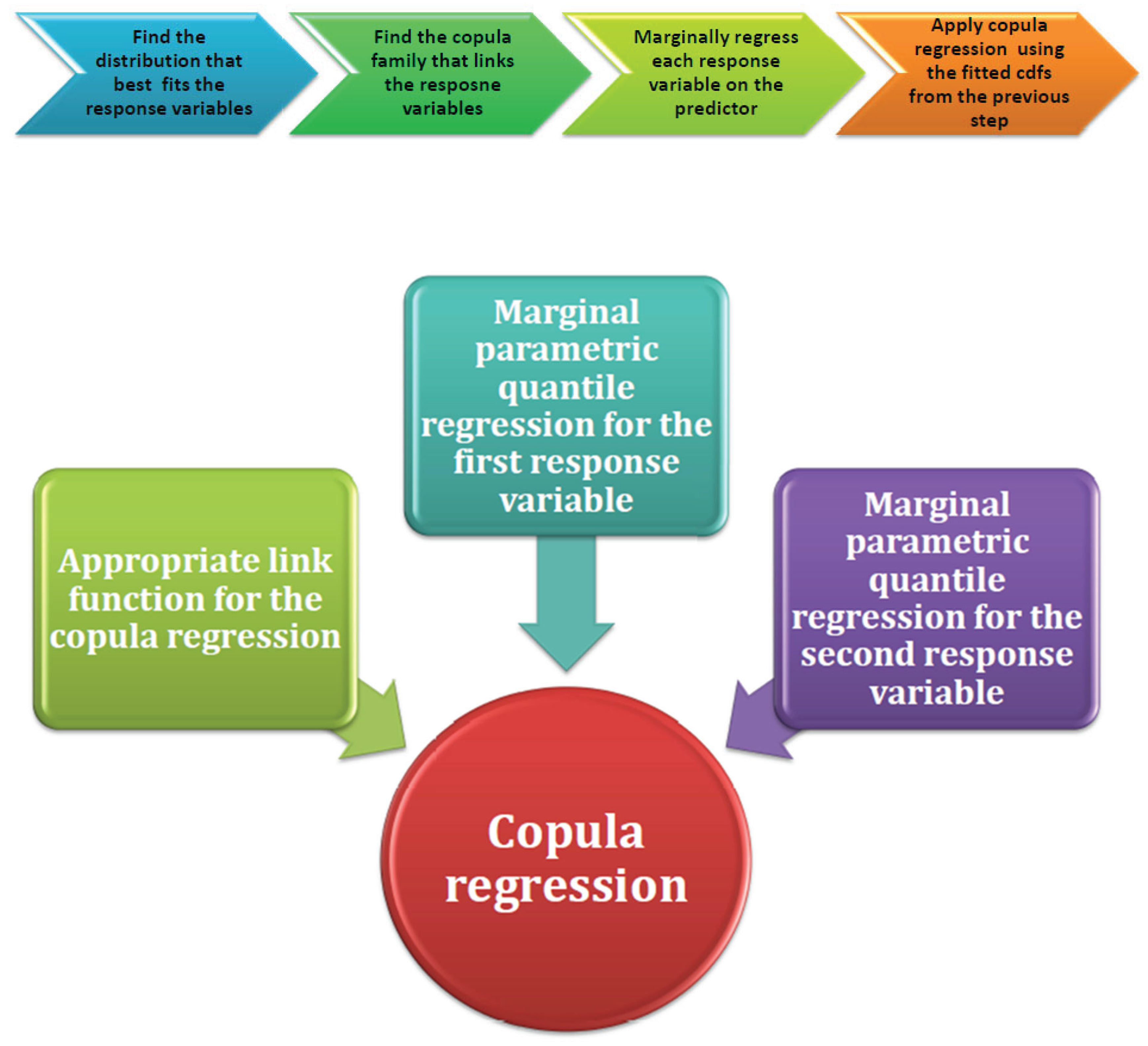
These illustrated flow diagrams show the steps to follow in applying parametric copula regression model.
The water quality indicator is computed as the self-reported approval with water quality and is signified by the percentage of people who report being satisfied with the quality of water as regards safety and cleanliness. The values of the water quality data are0.92, 0.92, 0.79, 0.9 ,0.62, 0.82, 0.87, 0.89, 0.93, 0.86, 0.97, 0.78, 0.91, 0.67, 0.81, 0.97, 0.8, 0.77, 0.77, 0.87, 0.82, 0.83, 0.83, 0.85, 0.75, 0.91, 0.85, 0.98, 0.82, 0.89, 0.81, 0.93, 0.76, 0.97, 0.96, 0.62, 0.82, 0.88, 0.7, 0.62, 0.72.
The quality of support network indicator measures the availability and reliability of help offered as a social support of friends, family, or community members to individuals who can rely on in time of need, and it is expressed as the percentage of people who report having someone they can count on for this support. The values of the quality support network are0.93, 0.92, 0.9, 0.93, 0.88, 0.8, 0.82, 0.96, 0.95, 0.95, 0.96, 0.94, 0.9, 0.78, 0.94, 0.98, 0.96, 0.95, 0.89, 0.89, 0.8, 0.92, 0.89, 0.91, 0.77, 0.94, 0.95, 0.96, 0.94, 0.87, 0.95, 0.95, 0.93, 0.94, 0.94, 0.85, 0.93, 0.94, 0.83, 0.89, 0.89.
The life expectancy indicator refers to the average number of years a person can expect to live based on current mortality rates and it is represented as a single number expressing the expected lifespan at birth, the values of the life expectancy data are 83, 82, 82.1, 82.1, 80.6, 76.7, 80.5, 79.3, 81.5, 78.8, 82.1, 82.9, 81.4, 81.7, 76.4, 83.2, 82.8, 82.9, 83.6, 84.4, 83.3, 75.5, 76.4, 82.7, 75.1, 82.2, 82.1, 83, 78, 81.8, 77.8, 81.6, 83.9, 83.2, 84, 78.6, 81.3, 78.9, 75.9, 73.2, 64.2.
First Step of Algorithm: The Distribution of the Response Variables.
The 2 response variable are distributed as MBUR with the following PDF , CDF and quantile functions, respectively: , and the quantile is
Figure 1 shows the boxplot of the response variables. Figure 2 shows the scatter plot between the two response variables. Figure 3 shows the scatter plot between the life expectancy water quality as well as the quality of support network. Figure 4 shows the fitted MBUR PDFs for both variables. Table 1 shows the descriptive statistics of the two response variables. Table 2 shows the Kendall Tau coefficient between the response variables. And Table 3 shows the statistical indices of both variables fitting MBUR distribution. The Kendall tau between water quality and life expectancy is 0.2859 and its statistically significant with p-value of 0.0099 while the Kendall tau between the quality of support network and the life expectancy is 0.2079 and it is statistically insignificant as the p-value is 0.0667. Although the distribution of the predictor does not affect the regression model, it is distributed as Kumaraswamy distribution as well as Beta distribution. But Kumaraswamy better fits the data rather than the Beta distribution as it has higher value of the Log-likelihood and more negative values of AIC, CAIC, BIC, and HQIC than the Beta distribution. To conduct the analysis, the predictor was transformed by dividing each value by 100 then taking the log of the result.
Table 1 depicts that the 2 response variables show left skewness that is more obvious for the quality of support network than that of the water quality. The quality of support network shows more leptokurtic shape than the shape of the water quality. Table 2 illuminates that both variables show significant positive dependence as seen by significant Kendall Tau coefficient
Table 3 highlights that the two variables fit the median based unit Rayleigh as null hypothesis fail to reject the tested MBUR distribution. Figure 4 shows the histogram and the fitted PDF curves for each response variable.
Second Step of Algorithm: The Copula Family That Links the Response Variables.
The response variables fit the Gumbel copula family. The theoretical tau is 0.3904 and the estimated dependency parameter is 1.6403. The estimated Cramer Von Mises (CVM) is 0.2154, the while . The Log-likelihood is 6.5649. Sampling from the fitted Gumbel copula using the Metropolis Hasting algorithm yielded a sampling distribution of the estimated tau with the 2.5th and 97.5th empirical quantiles being 0.2405 and 0.5432 respectively, a sampling distribution of the estimated dependency parameter with 2.5th and 97.5th empirical quantiles being 1.3166 and 2.1905 respectively, and a sampling distribution of the estimated CVM with 2.5th and 97.5th empirical quantiles being 0.0344 and 0.1754 respectively. Figure 5 shows the P-P plot of the theoretical vs the empirical Gumbel copula.
Figure 5.
Shows the P-P plot of the empirical copula vs the theoretical copula. The theoretical copula shows near perfect alignment of the lower part and the central part with the diagonal than the upper part.
Figure 5.
Shows the P-P plot of the empirical copula vs the theoretical copula. The theoretical copula shows near perfect alignment of the lower part and the central part with the diagonal than the upper part.
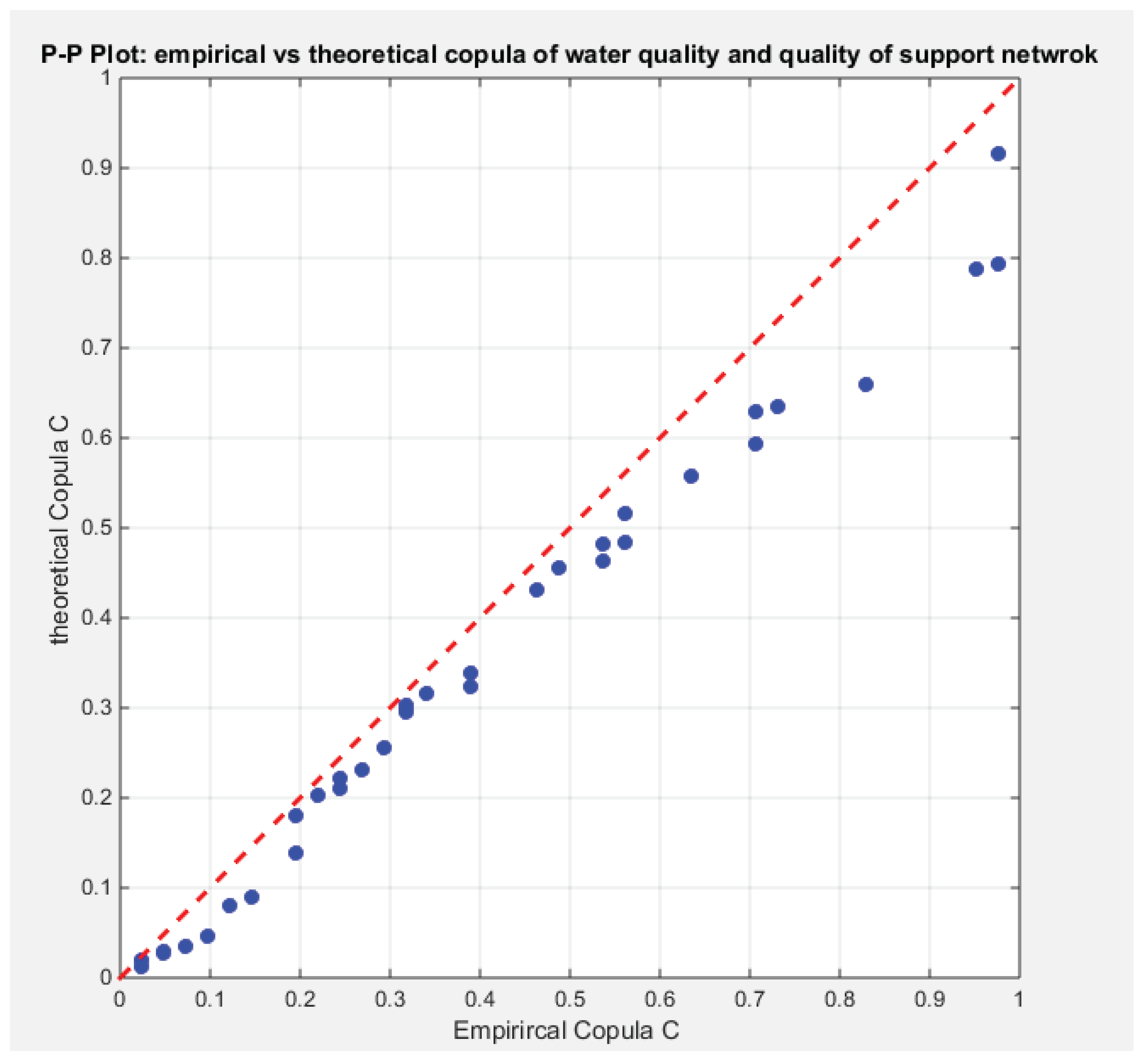
Figure 6.
Shows the sampling distribution of the Kendall Tau coefficient. The estimated tau is 0.3904 and it lies between the 2.5th and 97.5th empirical quantile. The null hypothesis testing the estimated tau is failed to be rejected.
Figure 6.
Shows the sampling distribution of the Kendall Tau coefficient. The estimated tau is 0.3904 and it lies between the 2.5th and 97.5th empirical quantile. The null hypothesis testing the estimated tau is failed to be rejected.
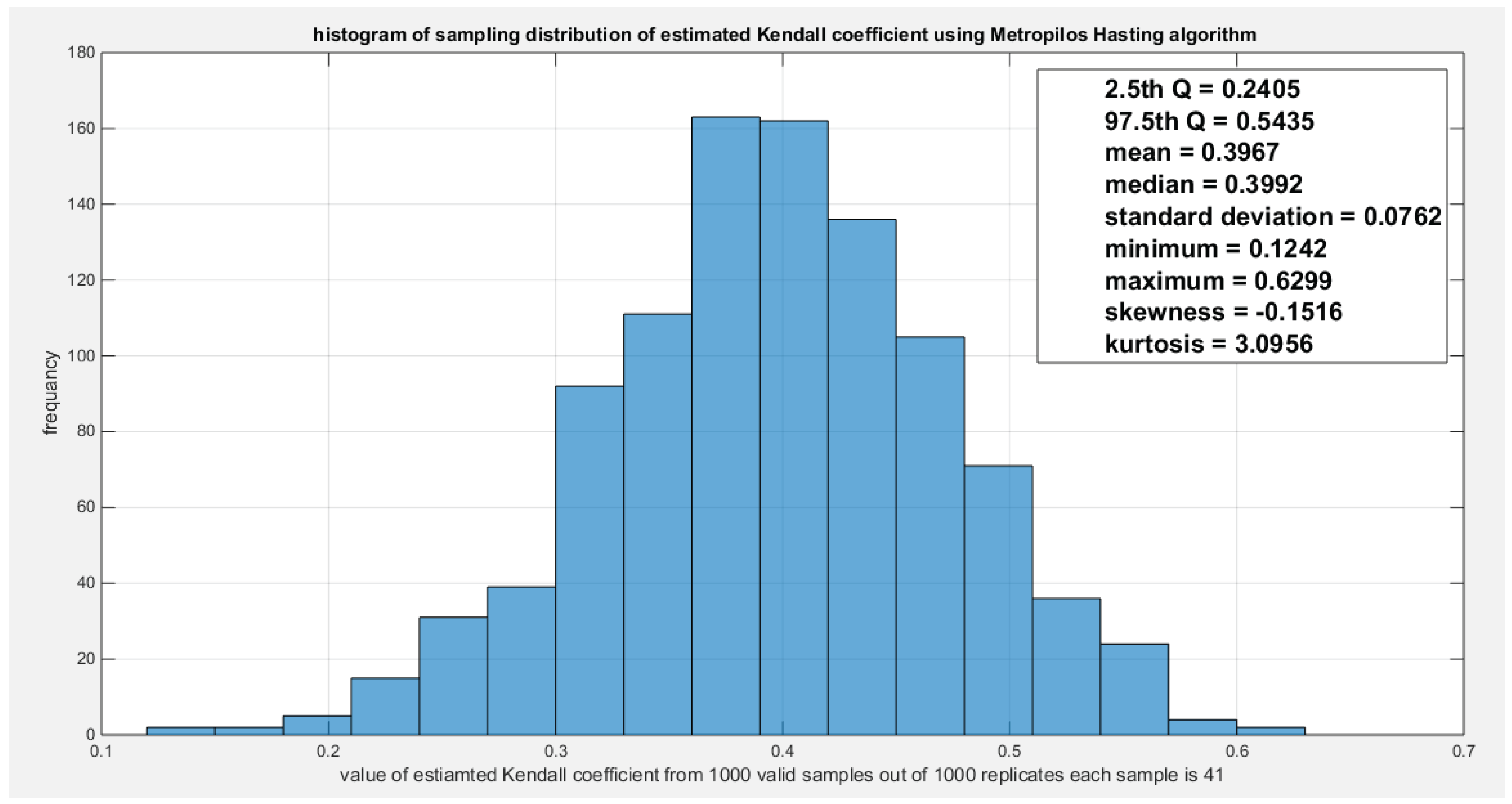
Figure 7, Figure 8 and Figure 9 show the sampling distributions obtained from the Metropolis Hasting algorithm for testing estimated tau, estimated dependency parameter, and the estimated CVM test. And the null hypothesis fails to reject any of the tested estimates. Hence the GoF tests for the Gumbel copula are illustrated and subsequently the two variables fit the Gumbel copula well.
Third Step of Algorithm: The Marginal Parametric Quantile Regression
As the response variables are negatively skewed, the logit link function and the log-log complementary link function can be considered as a good candidate to reparameterize the alpha parameter in the MBUR PDF. Both functions are monotone increasing functions. Hence applying the median parametric regression model to regress the water quality variable on the life expectancy variable as well as regressing the quality of support network on the life expectancy gives estimate of the alpha parameter for each observation. This is called the marginal regression model of each response variable on the predictor. The estimated alpha parameters of the marginal MBUR are utilized to acquire the fitted CDF for each marginal (or variable), these estimated CDF will be utilized in the copula regression part in which the dependency parameter of the Gumbel copula is defined in terms of each observation by the help of a link function that ensure that the dependency parameter is more than one.
Reparameterize the PDF and CDF of MBUR using the quantile function where c is . U represents the chosen percentile, in this analysis the author uses the median so u=0.5 and
As y is the median corresponding to u=0.5 then; replacing this u into the c equation, the c will also be 0.5. Using the logit function of the median which is called and
where n is the number of cases and k is the number of variables. Logit median is a linear combination of variables.
Replace this parameter in the Log-Likelihood function and the coefficients can be obtained by the MLE, the author used the derivative free algorithm; Nelder Mead simplex optimizer in MATLAB.
A link function other than the logit which is also monotonically increasing is the log-log (1-median) , hence the median is and . The author used the 2 link models and compare between them.
The results of the marginal regression of each of the response variable on the predictor are shown in 2 tables; each table represents the results gained from utilizing a specific link function. Table 4 shows the results of regressing the response variable on the predictor using the logit link function. While, Table 5 shows the results of regressing the response variable on the predictor using the log-log complementary link function.
Figure 9 shows the estimated curve for regressing the water quality and the quality of support network on transformed life expectancy. The graph supports the results of the significant effect of life expectancy on the water quality than its significant effect on the quality of support network. The pink curve is steeper than the blue one. Although the log-likelihood has higher value for the model incorporating the quality of support network than the model incorporating the water quality but the LRT points to the significance of the water quality over the quality of support network which is supported by Wald test statistics results and graph in Figure 9. The more the life expectancy is the more satisfaction of water quality is.
Figure 10 shows the QQ plot of the empirical quantiles versus the theoretical quantiles. The logit model regressing the water quality on the life expectancy has a curve of randomized quantile residuals that shows near perfect alignment with the diagonal all through its course, while the curve of the Cox-Snell residuals is mainly aligned with the diagonal at its lower tail and its center. Figure 11 shows the QQ plot for the logit model curve regressing the quality of support network on the life expectancy which has less efficient alignment with the diagonal as regards residuals, the randomized quantile residuals and the Cox-Snell residuals. Figure 12 and Figure 13 show the scatter plot of the predictor (transformed) and the both types of residuals (randomized quantile and Cox-Snell). There is no nonlinear relationship between the predictor and the residuals. This relationship can be expressed in Kendall tau coefficient as -0.1093 and associated p-value=0.3225 for the response variable (water quality) while it is -0.1104 and associated p-value=0.3171 for the response variable (quality of support network). These values are identical for both types of residuals for each response variable. So there is no evidence for dependency between the predictor and the residuals.
Figure 14 shows the estimated curve for regressing the water quality and the quality of support network on transformed life expectancy. The graph supports the results of the significant effect of life expectancy on the water quality than its significant effect on the quality of support network. The pink curve is steeper than the blue one. Although the log-likelihood has higher value for the model incorporating the quality of support network than the model incorporating the water quality but the LRT points to the significance of the water quality over the quality of support network which is supported by Wald test statistics results and graph in Figure 14. The more the life expectancy is the more satisfaction of water quality is.
Figure 15 shows the QQ plot of the empirical quantiles versus the theoretical quantiles. The log-log complementary model regressing the water quality on the life expectancy has a curve of randomized quantile residuals that shows near perfect alignment with the diagonal all through its course, while the curve of the Cox-Snell residuals is mainly aligned with the diagonal at its lower tail and its center. Figure 16 shows the QQ plot for the log-log complementary model curve regressing the quality of support network on the life expectancy which has less efficient alignment with the diagonal as regards the residuals, the randomized quantile residuals and the Cox-Snell residuals. Figure 17 and Figure 18 show the scatter plot of the predictor (transformed) and both types of residuals (the randomized quantile and the Cox-Snell). There is no nonlinear relationship between the predictor and the residuals. This relationship can be expressed in Kendall tau coefficient as -0.1093 and associated p-value=0.3225 for the response variable (water quality) while it is -0.1104 and associated p-value=0.3171 for the response variable (quality of support network). These values are identical for both types of residuals for each response variable. So there is no evidence for dependency between the predictor and the residuals.
Fourth Step of Algorithm: The Copula Parametric Quantile Regression
The quantile parametric copula regression is a copula regression model utilizing the fitted marginal CDFs obtained from the fitted marginal quantile parametric MBUR regression models. Regressing each copula dependency parameter on the corresponding observation with the aid of the link function where h is the link function that ensures the dependency parameter is larger than one. The author used the Inference Function of Margin (IFM) and the Nelder Mead algorithm of MATLAB as an optimizer. The Gumbel copula PDF is
where , reparameterize the dependency parameter in this copula PDF with the , in other words, replace the right hand side of the link function in copula PDF and optimize. The u and v are the fitted CDFs obtained from the quantile marginal regression step. The relation between the theta dependence parameter and Kendall tau is . After applying the copula regression in this step, there will be a value of theta for each , and in Table 6, the mean of this tau is recorded as the mean of theoretical tau while the empirical tau is calculated from the u and v.
The Gumbel copula CDF is
Table 6 enlightens the results of copula regression part using log-log complementary model and the logit model. The AIC, CAIC, BIC, HQIC for the logit model are less than those of the log-log complementary model. CVM for the logit is less than that of the log-log complementary model. The LRT is statistically significant for the logit model than the LRT for the complementary model. Figure 19, Figure 20 and Figure 21 explicate the histogram of the parametric bootstrap sampling of the estimated CVM, estimated intercept and the estimated slope, respectively obtained from the logit model depicting the descriptive statistics as shown in each figure. Figure 22 elucidates that the estimated LRT value (4.3426) lies between the 2.5th and 97.5th quantile of the parametric bootstrap sampling distribution. The slope is 5 % statistically significant using the logit model. The log-log complementary model shows 30% statistical significance of the estimated CVM, estimated intercept, and estimated slope using the parametric bootstrap sampling distribution as expounded in Figure 23, Figure 24 and Figure 25. Although, the estimated CVM is statistically significant at 5% significance level as shown from parametric sampling distribution in Figure 26, the estimated slope is statistically significant at 5% significant level as shown from the non-parametric bootstrap sampling distribution in Figure 27; which is less powerful than the parametric bootstrap sampling distribution. Figure 28 shows the parametric bootstrap sampling of the LRT illuminating that the LRT is significant at 30% significant level for the log-log complementary model.
From the above results, the logit model demonstrates better fit for the effect of predictor (life expectancy) on the dependency between the 2 response variables (water quality and quality of support network) than the log-log complementary model. The logit model is significant at 5% significant level while the log-log model is significant at 30 % significant level. Figure 29 and Figure 30 show that as the life expectancy increases, the dependency between water quality and quality of support network decrease for both the logit and the complementary model. Figure 31 and Figure 32 show the PP plot of the fitted theoretical copula vs. the empirical copula of the second regression part, the copula regression. Both graphs show near perfect alignment all through the course except of 6 observations which are a little bit far away from the diagonal.
5. Conclusions
The water quality and the quality of support network are linked together via Gumbel copula and they are strongly dependent to each other. They show very strong positive dependency, if one enlarges the other also enlarges, and this is logic as in the community where their residences have high expression about the good quality of the water supplies, they are more likely to support each other at the time of needs and crises. Marginally regressing the water quality on the life expectancy shows significant positive nonlinear relationship between the response and the predictor reflecting the community where their population has long life, this increase the satisfactions of the cleanliness of the water supplies. Also as the life expectancy increase, this increase the support the individuals in the community can have in times of need, but this effect of life expectancy on the quality of support network is not statistically significant as the effect of life expectancy on the water quality. But the dependency between water quality and quality of support weakens as the life expectancy increases. Using the Logit link function for the marginal median regression model shows better statistical indices than the log-log complementary link function. And this has a reflection on the second part, the parametric median copula regression part, where the indices are significant at 5% confidence level than the 30% confidence level attained while using the log-log complementary link function.
The significant effect of life expectancy on water quality can be interpreted as elderly have significant high expression of their satisfaction about the water quality and they do not show this significant high satisfaction about the quality of support network although it is present but not that significant. As the life expectancy does not have the same positive significant effect on both response variables, the dependency between the 2 response variables may weaken as the life expectancy increases. This can be interpreted as the percentage of people who can express their great satisfaction with water quality and the presence of support network are mainly the young (less life expectancy) while the elderly are the percentage who express less satisfaction with water quality and support network and this may be because they live alone so they are not receiving enough care for their water cleanliness and support so they have this impact by expressing less satisfaction for both response variables together. Also the source of water or the acquisition of the clean water all can make the expression of satisfaction vary in elderly. If they can buy the well-formed bottles of clean water or they have to check for the cleanliness for the household water supply.
This study introduces an innovative parametric copula regression framework that intricately captures the multifaceted relationship between two response variables while conditioning on a covariate. Departing from traditional regression methodologies, which often treat each response in isolation, this pioneering approach plunges into the depths of interdependencies that weave between outcomes, harnessing a dynamic parametric copula. The properties and structural nuances of this copula evolve as the predictor varies, enriching the analysis with its adaptability. Applying Sklar’s theorem, the complex joint conditional distribution is masterfully unraveled into a series of marginal regression models, seamlessly coupled with a dependence function signified by a Gumbel copula. In this framework, the copula parameter is elegantly modeled as a smooth function of the covariate, allowing for a dynamic interaction of dependence that transforms across different levels of the predictor. To estimate parameters, the inference function for margins (IFM) method was employed, ensuring robust computational stability along with impressive asymptotic efficiency. A comprehensive set of diagnostic checks based on residual analysis not only affirmed the adequacy of the fitted marginal models, but also validated the copula’s dependence structure, underscoring the reliability of the framework. Empirical findings have illuminated the model's exceptional ability to encapsulate the distinctive behaviors of marginal responses, as well as the evolving patterns of dependence between them. One striking observation revealed that the dependence parameter tended to diminish as the predictor values increased, indicating that the two outcomes became less tightly intertwined amid rising predictor levels. This flexible modeling architecture offers profound insights into how covariates influence not just individual responses but also their intricate interconnected dynamics. Such a feature proves particularly valuable in fields like finance, hydrology, and biostatistics, where grasping the co-movement between outcomes is crucial for informed decision-making and strategic planning.
6. Future Work
The proposed framework presents numerous opportunities for further development and expansion. Future research could explore the implementation of higher-dimensional copulas, which would allow for the modeling of interactions among more than two response variables concurrently. This could be particularly useful in complex systems where multiple factors are interrelated. Additionally, the use of semiparametric link functions could be investigated to enhance the flexibility in modeling the dependent relationships among variables. This approach would enable researchers to better accommodate various distributions and non-linear associations, providing a richer analysis of multivariate data. Another promising avenue for future work is the incorporation of time-varying copula parameters. This adaptation would be essential for capturing dynamic dependence structures in longitudinal or temporal datasets, where relationships between variables may evolve over time. By allowing the dependence parameters to change, the model could more accurately reflect real-world phenomena where relationships are not static. Overall, the parametric copula regression model stands out as a powerful and interpretable tool for investigating multivariate conditional dependence. It effectively bridges the traditional methods of classical regression with the advanced techniques of contemporary dependence modeling, thereby offering a comprehensive framework for analyzing the intricate relationships between multiple variables.
Author Contributions
AI (Iman Attia) carried the conceptualization by formulating the goals, aims of the research article, formal analysis by applying the statistical, mathematical and computational techniques analyze the real data, carried the methodology by creating the model, software programming and implementation, supervision, writing, drafting, editing, preparation, and creation of the presenting work.
Funding
No funding resource. No funding roles in the design of the study and collection, analysis, and interpretation of data and in writing the manuscript are declared
Informed Consent Statement
Not applicable
Data Availability Statement
Data sharing is not applicable to this article as no new data were created or analyzed in this study.
Conflicts of Interest
The author declares no competing interests of any type.
References
- H. Joe, Dependence Modeling with Copulas. London: CRC Press, 2014.
- P. D’Urso, L. De Giovanni, and V. Vitale, “A D-vine copula-based quantile regression model with spatial dependence for COVID-19 infection rate in Italy,” Spatial Statistics, vol. 47, p. 100586, Mar. 2022. [CrossRef]
- N. Hans, N. Klein, F. Faschingbauer, M. Schneider, and A. Mayr, “Boosting Distributional Copula Regression,” Biometrics, vol. 79, no. 3, pp. 2298–2310, Sept. 2023. [CrossRef]
- G. Briseño Sanchez, N. Klein, H. Klinkhammer, and A. Mayr, “Boosting distributional copula regression for bivariate binary, discrete and mixed responses,” Stat Methods Med Res, vol. 34, no. 5, pp. 887–902, May 2025. [CrossRef]
- J. Stöber, H. G. Hong, C. Czado, and P. Ghosh, “Comorbidity of chronic diseases in the elderly: Patterns identified by a copula design for mixed responses,” Computational Statistics & Data Analysis, vol. 88, pp. 28–39, Aug. 2015. [CrossRef]
- Y. Liu, Y. Zhou, Y. Chen, D. Wang, Y. Wang, and Y. Zhu, “Comparison of support vector machine and copula-based nonlinear quantile regression for estimating the daily diffuse solar radiation: A case study in China,” Renewable Energy, vol. 146, pp. 1101–1112, Feb. 2020. [CrossRef]
- T. Emura, C. L. Sofeu, and V. Rondeau, “Conditional copula models for correlated survival endpoints: Individual patient data meta-analysis of randomized controlled trials,” Stat Methods Med Res, vol. 30, no. 12, pp. 2634–2650, Dec. 2021. [CrossRef]
- K. Wang and W. Shan, “Copula and composite quantile regression-based estimating equations for longitudinal data,” Ann Inst Stat Math, vol. 73, no. 3, pp. 441–455, June 2021. [CrossRef]
- D. Petti, A. Eletti, G. Marra, and R. Radice, “Copula link-based additive models for bivariate time-to-event outcomes with general censoring scheme,” Computational Statistics & Data Analysis, vol. 175, p. 107550, Nov. 2022. [CrossRef]
- R. A. Parsa and S. A. Klugman, “Copula regression,” Variance 5(1), 45–54 (2011), vol. 5, no. 1, pp. 45–54, 2011.
- X. Chen, R. Koenker, and Z. Xiao, “Copula-based nonlinear quantile autoregression,” Econometrics Journal, vol. 12, pp. S50–S67, Jan. 2009. [CrossRef]
- H. J. Wang, X. Feng, and C. Dong, “COPULA-BASED QUANTILE REGRESSION FOR LONGITUDINAL DATA,” STAT SINICA, 2018. [CrossRef]
- H. Noh, A. E. Ghouch, and T. Bouezmarni, “Copula-Based Regression Estimation and Inference,” Journal of the American Statistical Association, vol. 108, no. 502, pp. 676–688, June 2013. [CrossRef]
- D. Kraus and C. Czado, “D-vine copula based quantile regression,” Computational Statistics & Data Analysis, vol. 110, pp. 1–18, June 2017. [CrossRef]
- E. Bouyé and M. Salmon, “Dynamic copula quantile regressions and tail area dynamic dependence in Forex markets,” The European Journal of Finance, vol. 15, no. 7–8, pp. 721–750, Dec. 2009. [CrossRef]
- A. Rokhsari, N. Doodman, and H. Tanha, “Effects of Coronavirus Pandemic on U.S Economy: D-Vine Regression Copula Approach,” Scientia Iranica, vol. 0, no. 0, pp. 0–0, Oct. 2022. [CrossRef]
- L. Fu and Y.-G. Wang, “Efficient parameter estimation via Gaussian copulas for quantile regression with longitudinal data,” Journal of Multivariate Analysis, vol. 143, pp. 492–502, Jan. 2016. [CrossRef]
- M. Tian and H. Ji, “GARCH copula quantile regression model for risk spillover analysis,” Finance Research Letters, vol. 44, p. 102104, Jan. 2022. [CrossRef]
- J. Sun, E. W. Frees, and M. A. Rosenberg, “Heavy-tailed longitudinal data modeling using copulas,” Insurance: Mathematics and Economics, vol. 42, no. 2, pp. 817–830, Apr. 2008. [CrossRef]
- V. R. Craiu and A. Sabeti, “In mixed company: Bayesian inference for bivariate conditional copula models with discrete and continuous outcomes,” Journal of Multivariate Analysis, vol. 110, pp. 106–120, Sept. 2012. [CrossRef]
- N. Klein, T. Kneib, G. Marra, R. Radice, S. Rokicki, and M. E. McGovern, “Mixed binary-continuous copula regression models with application to adverse birth outcomes,” Statistics in Medicine, vol. 38, no. 3, pp. 413–436, Feb. 2019. [CrossRef]
- P. Xue-Kun Song, “Multivariate Dispersion Models Generated From Gaussian Copula,” Scandinavian J Statistics, vol. 27, no. 2, pp. 305–320, June 2000. [CrossRef]
- T. Bedford and R. M. Cooke, “Probability Density Decomposition for Conditionally Dependent Random Variables Modeled by Vines,” Annals of Mathematics and Artificial Intelligence, vol. 32, no. 1–4, pp. 245–268, Aug. 2001. [CrossRef]
- A. K. Nikoloulopoulos and D. Karlis, “Regression in a copula model for bivariate count data,” Journal of Applied Statistics, vol. 37, no. 9, pp. 1555–1568, Sept. 2010. [CrossRef]
- G. Marra and K. Wyszynski, “Semi-parametric copula sample selection models for count responses,” Computational Statistics & Data Analysis, vol. 104, pp. 110–129, Dec. 2016. [CrossRef]
- H. Noh, A. E. Ghouch, and I. Van Keilegom, “Semiparametric Conditional Quantile Estimation Through Copula-Based Multivariate Models,” Journal of Business & Economic Statistics, vol. 33, no. 2, pp. 167–178, Apr. 2015. [CrossRef]
- M. De Backer, A. El Ghouch, and I. Van Keilegom, “Semiparametric copula quantile regression for complete or censored data,” Electron. J. Statist., vol. 11, no. 1, Jan. 2017. [CrossRef]
- N. Klein and T. Kneib, “Simultaneous inference in structured additive conditional copula regression models: a unifying Bayesian approach,” Stat Comput, vol. 26, no. 4, pp. 841–860, July 2016. [CrossRef]
- H. Dette, R. Van Hecke, and S. Volgushev, “Some Comments on Copula-Based Regression,” Journal of the American Statistical Association, vol. 109, no. 507, pp. 1319–1324, July 2014. [CrossRef]
- F. Alshenawy, “Using Tail Dependence on Copula-based Regression Models in Mixed Data,” The Egyptian Statistical Journal, vol. 68, no. 2, pp. 65–85, Dec. 2024. [CrossRef]
- R. M. Cooke, H. Joe, and B. Chang, “Vine copula regression for observational studies,” AStA Adv Stat Anal, vol. 104, no. 2, pp. 141–167, June 2020. [CrossRef]
- T. Bedford and R. M. Cooke, “Vines--a new graphical model for dependent random variables,” Ann. Statist., vol. 30, no. 4, Aug. 2002. [CrossRef]
- I. Attia, “A Novel One Parameter Unit Distribution: Median Based Unit Rayleigh: Properties and Estimations,” Oct. 07, 2024, Preprint.org. [CrossRef]
Figure 1.
Shows the boxplot of the two response variable; water quality and quality support network. Both variables demonstrate left skewness, being -0.6059 for water quality and -1.176 for the quality support network.
Figure 1.
Shows the boxplot of the two response variable; water quality and quality support network. Both variables demonstrate left skewness, being -0.6059 for water quality and -1.176 for the quality support network.

Figure 2.
Shows the scatter plot of the two response variables that exhibits significant positive dependency. The Kendall Tau is 0.03929 and p-value=0.0006.
Figure 2.
Shows the scatter plot of the two response variables that exhibits significant positive dependency. The Kendall Tau is 0.03929 and p-value=0.0006.
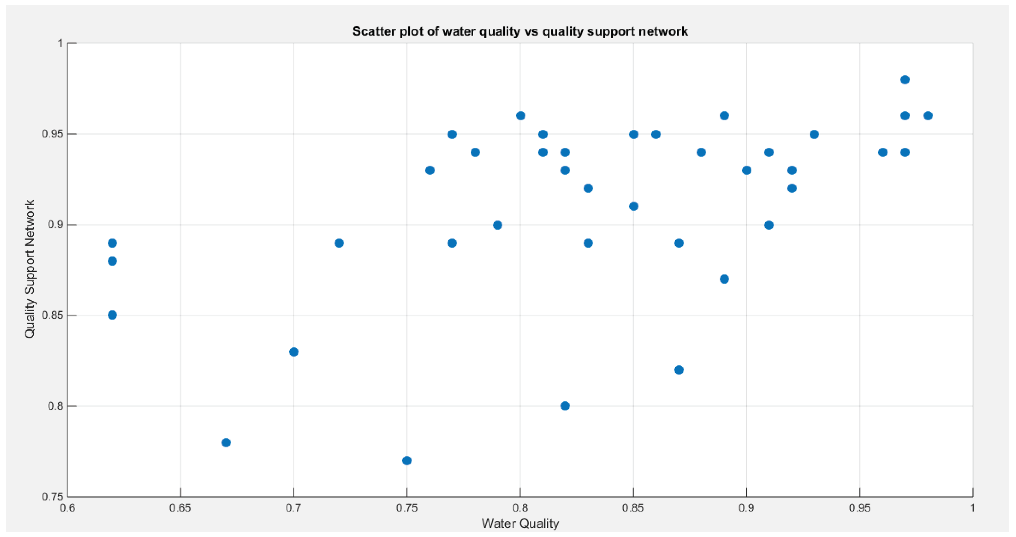
Figure 3.
Shows the non-linear relationship between the two response variables and the predictors, life expectancy (transformed). The Kendall tau between the water quality and the life expectancy (raw and not transformed) is statistically significant (tau= 0.2859, p-value=0.0099) while the Kendall tau between the quality of support network and the life expectancy (raw & not transformed) is statistically insignificant (tau=0.2079 p-value=0.0667).
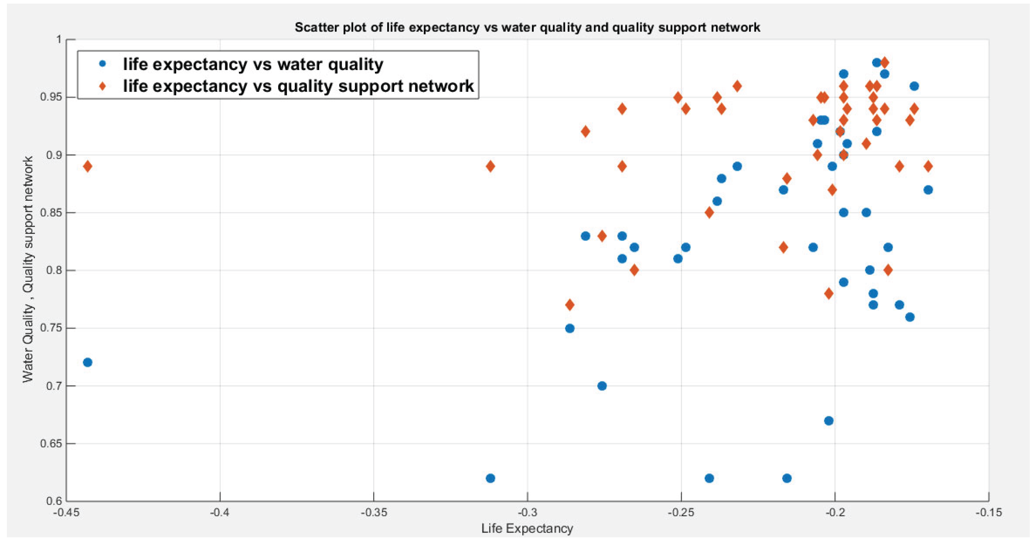
Figure 4.
Shows the fitted PDF of MBUR for both response variables.
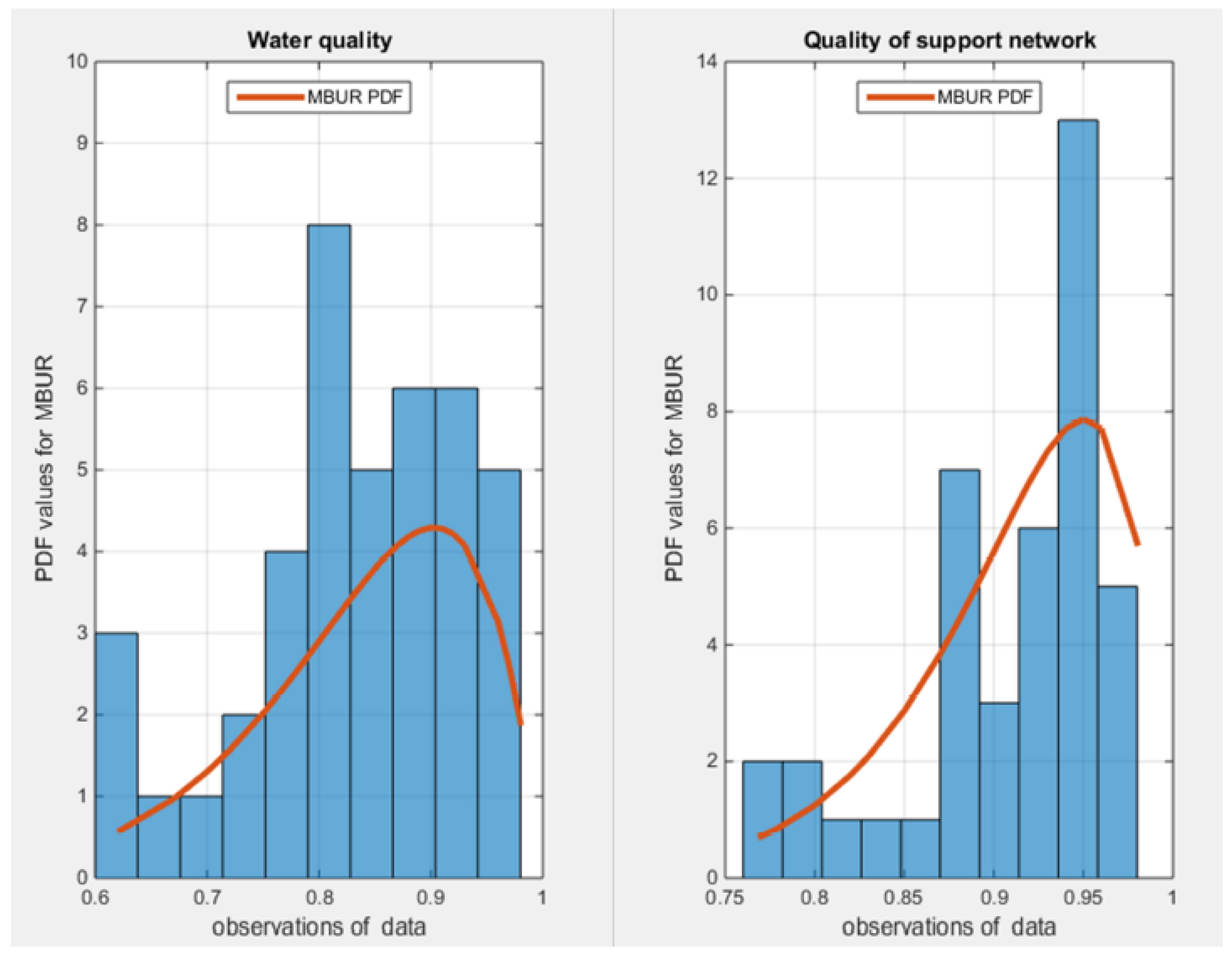
Figure 7.
Shows the sampling distribution of the estimated dependency parameter coefficient. The estimated tau is 1.6403 and it lies between the 2.5th and 97.5th empirical quantile. The null hypothesis testing the estimated dependency parameter is failed to be rejected.
Figure 7.
Shows the sampling distribution of the estimated dependency parameter coefficient. The estimated tau is 1.6403 and it lies between the 2.5th and 97.5th empirical quantile. The null hypothesis testing the estimated dependency parameter is failed to be rejected.
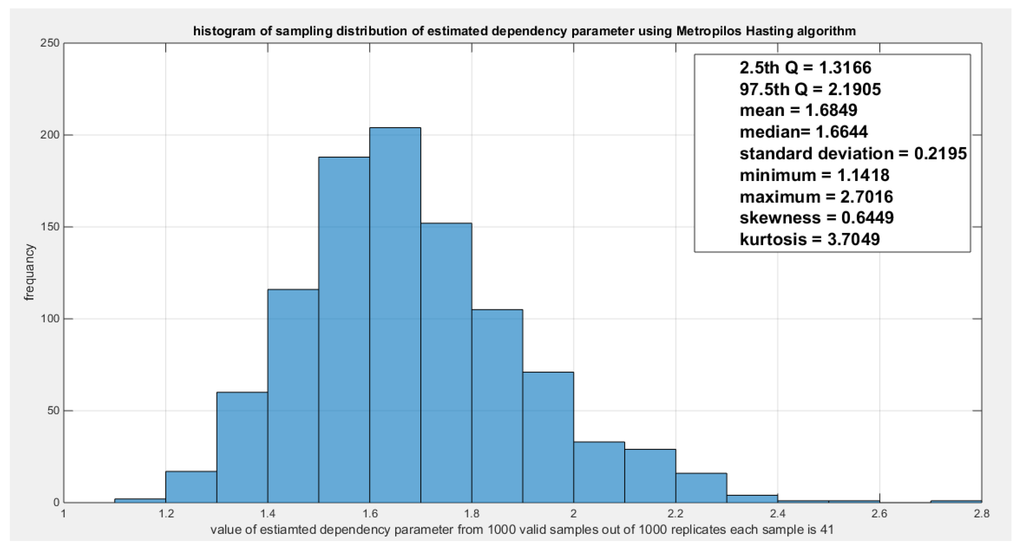
Figure 8.
Shows the sampling distribution of the estimated CVM. The estimated tau is 0.2154 and it lies between the 2.5th and 97.5th empirical quantile. The null hypothesis testing the estimated CVM is failed to be rejected.
Figure 8.
Shows the sampling distribution of the estimated CVM. The estimated tau is 0.2154 and it lies between the 2.5th and 97.5th empirical quantile. The null hypothesis testing the estimated CVM is failed to be rejected.
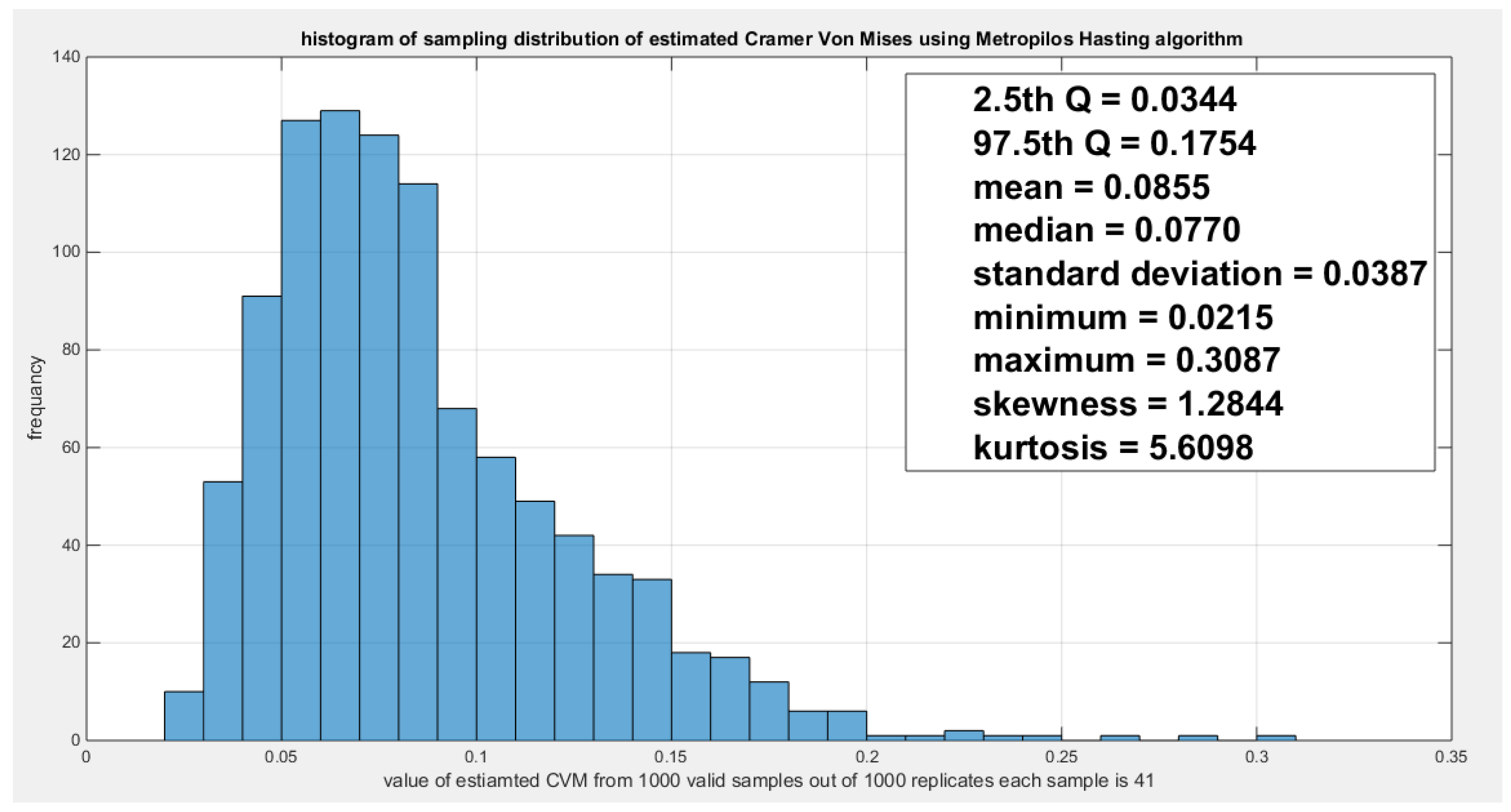
Figure 9.
Shows that the curve of the logit model regressing the water quality on life expectancy is steeper than the curve that models the regression of quality of support network on life expectancy.
Figure 9.
Shows that the curve of the logit model regressing the water quality on life expectancy is steeper than the curve that models the regression of quality of support network on life expectancy.
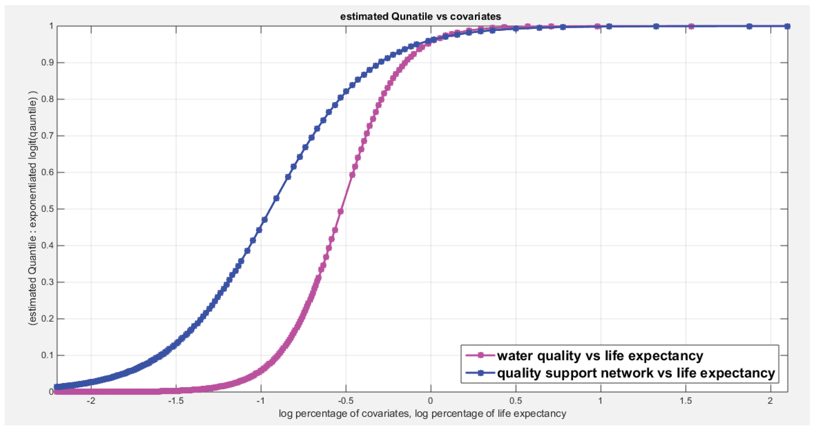
Figure 10.
Shows the QQ plot of the empirical vs. the theoretical quantiles for the logit model where the water quality is regressed on the life expectancy. The randomized quantile residuals show near perfect alignment all through the course of the curve in contrast to the Cox-Snell residuals which show more or less near alignment mainly in the lower tail and center of the curve than the upper tail.
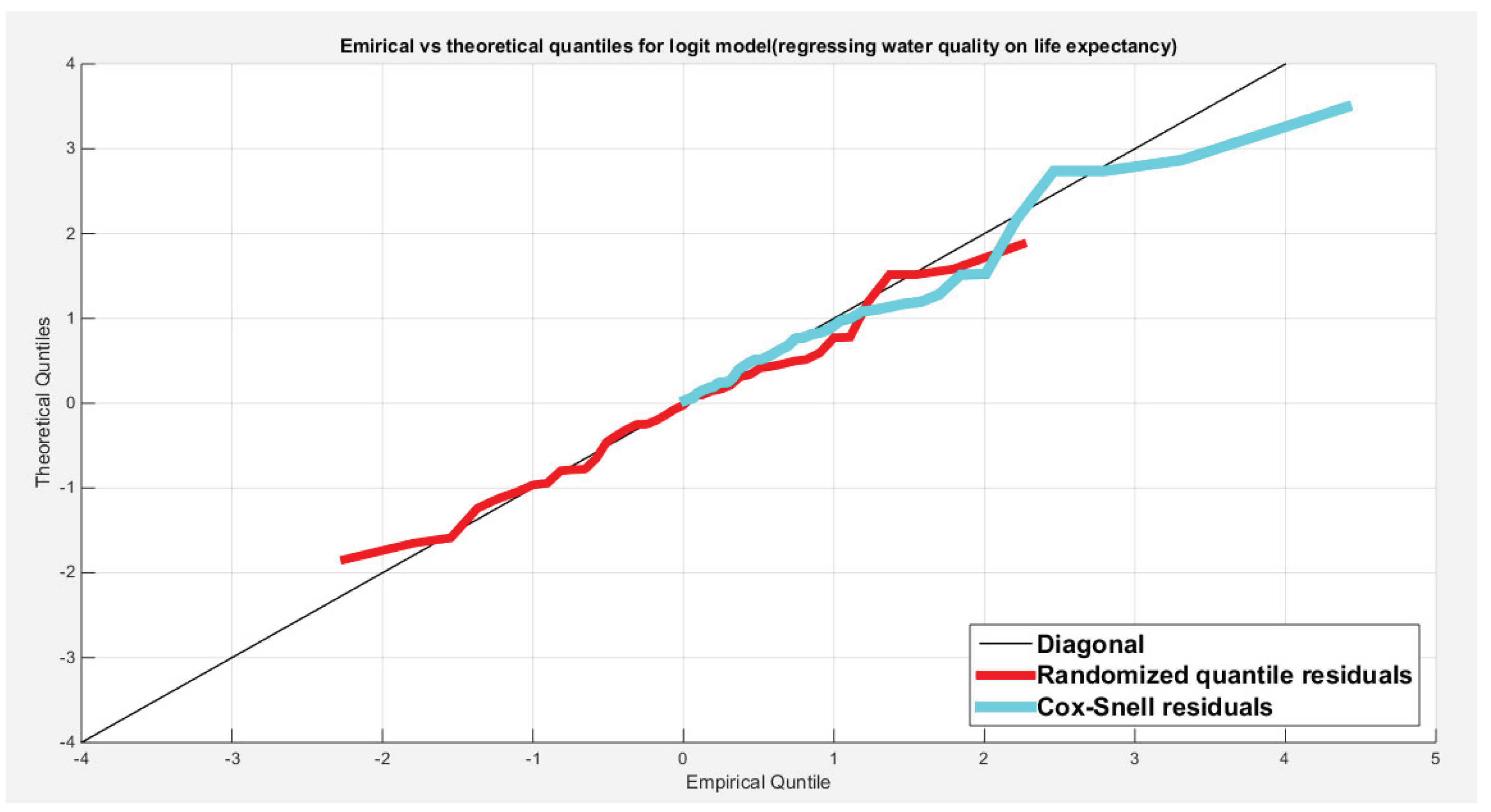
Figure 11.
Shows the QQ plot of the empirical vs. the theoretical quantiles for the logit model where the quality of support network is regressed on the life expectancy. The randomized quantile residuals show near perfect alignment at the lower part and the center of the curve. While the Cox-Snell residuals only depict near alignment at the lower tail.
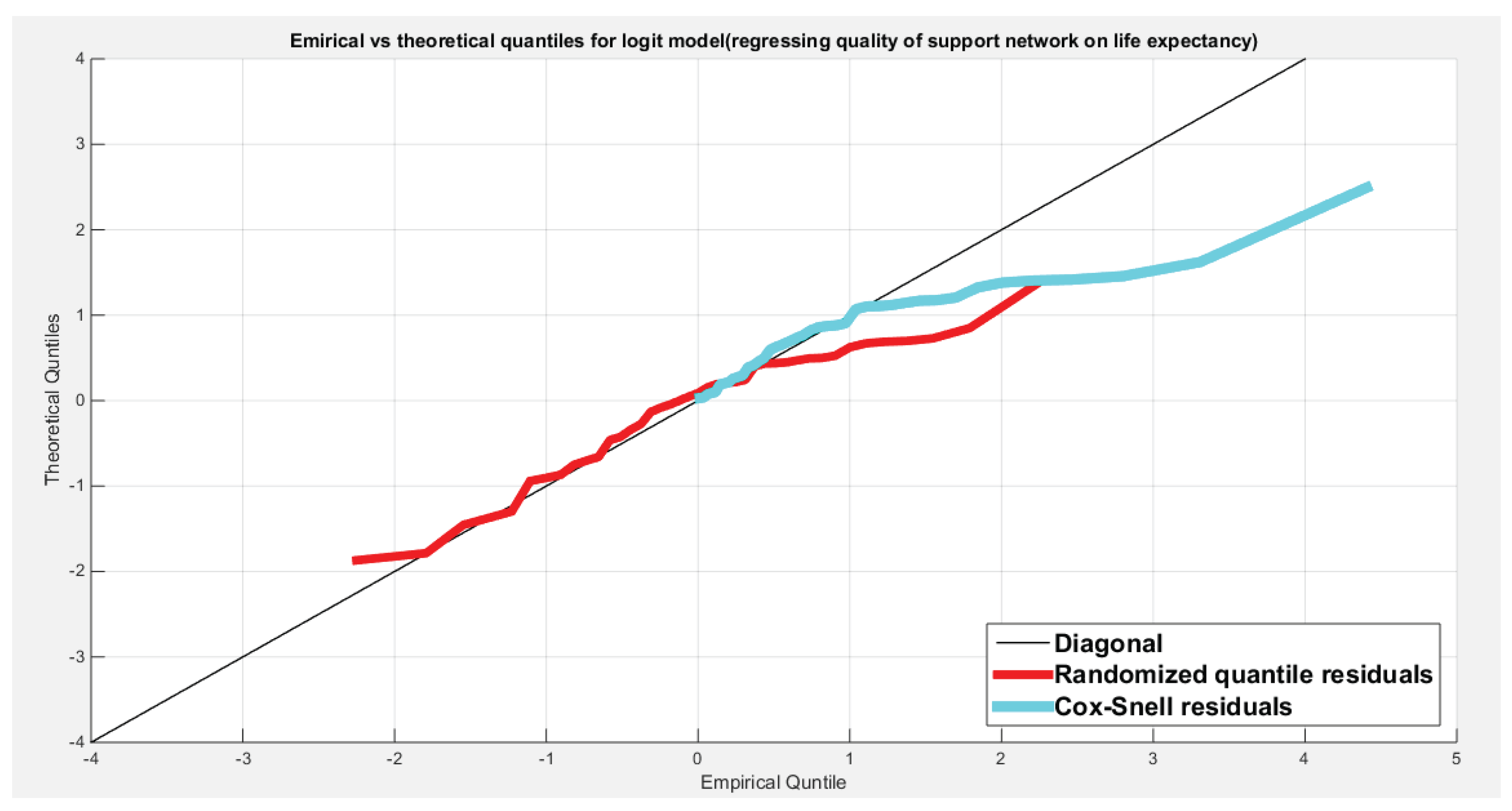
Figure 12.
Shows the scatter plot between the life expectancy predictor (transformed) and the randomized quantile residuals and Cox-Snell residuals for the logit model regressing the life expectancy on water quality. There is no specific trend or relationship between them and the scatter is random. No evidence of dependence between the predictor and the residuals of both types. The Kendall tau dependency parameter between the predictor and the residuals is -0.1093 with p-value= 0.3225 which is not statistically significant. These values are true for both types of residuals.
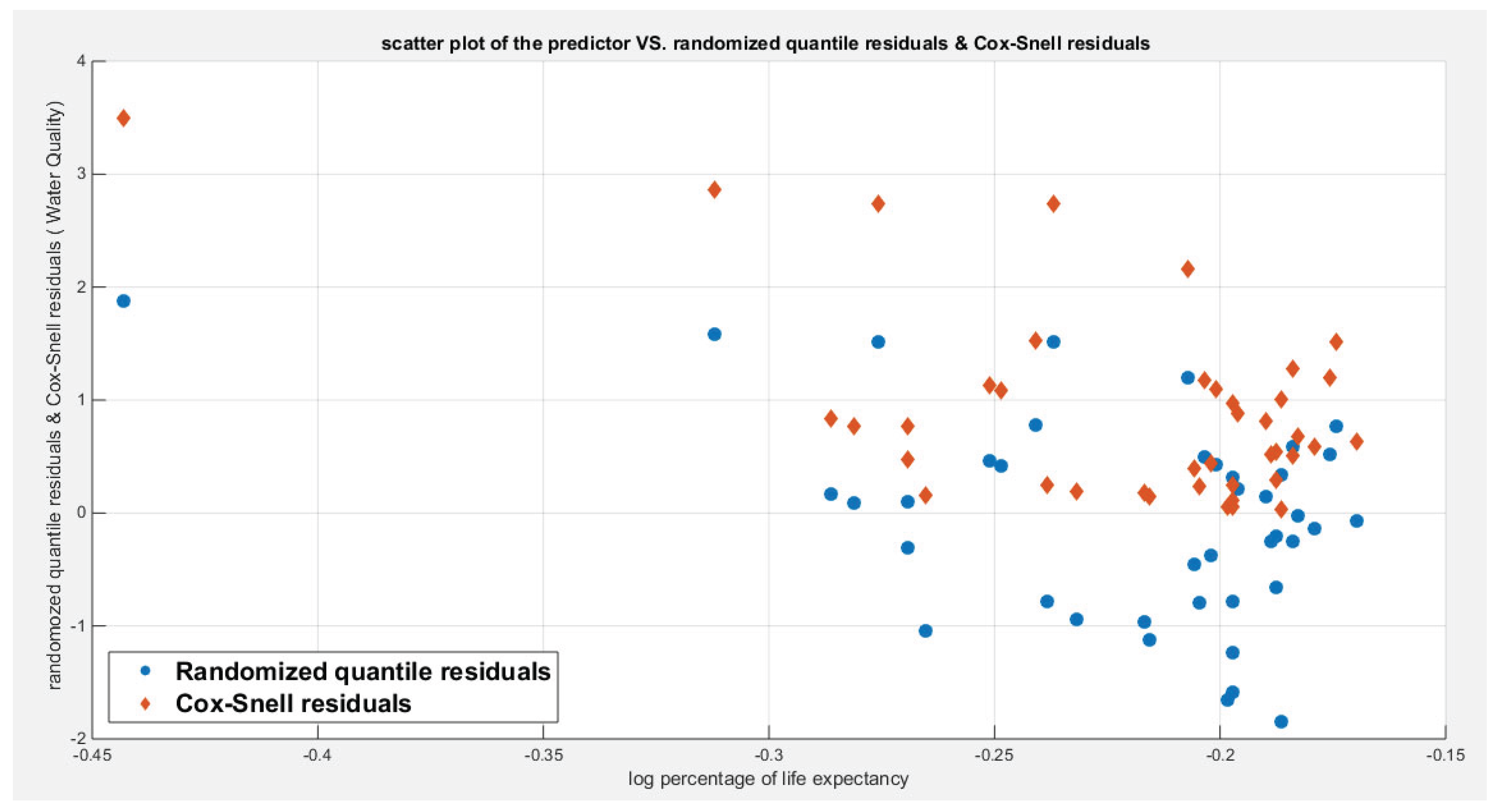
Figure 13.
Shows the scatter plot between the life expectancy predictor (transformed) and the randomized quantile residuals and Cox-Snell residuals for the logit model regressing the life expectancy on quality of support network . There is no specific trend or relationship between them and the scatter is random. No evidence of dependence between the predictor and the residuals of both types. The Kendall tau dependency parameter between the predictor and the residuals is -0.1104 with p-value= 0.3171 which is not statistically significant. These values are true for both types of residuals.
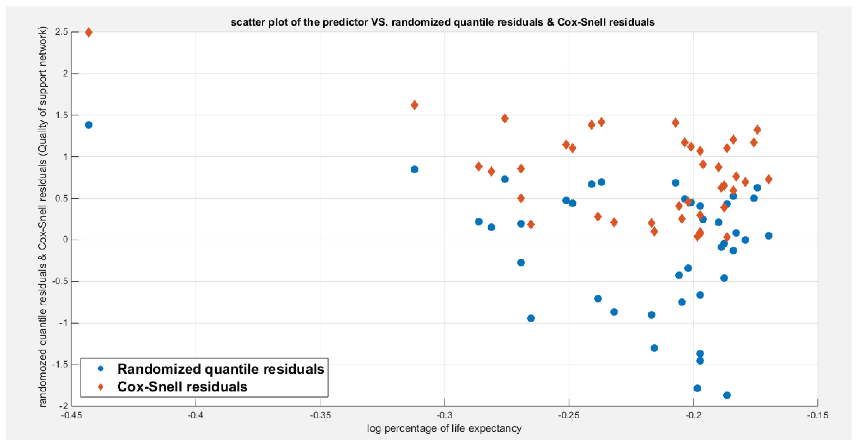
Figure 14.
Shows that the curve of the log-log complementary model regressing the water quality on life expectancy is steeper than the curve that models the regression of quality of support network on life expectancy.
Figure 14.
Shows that the curve of the log-log complementary model regressing the water quality on life expectancy is steeper than the curve that models the regression of quality of support network on life expectancy.
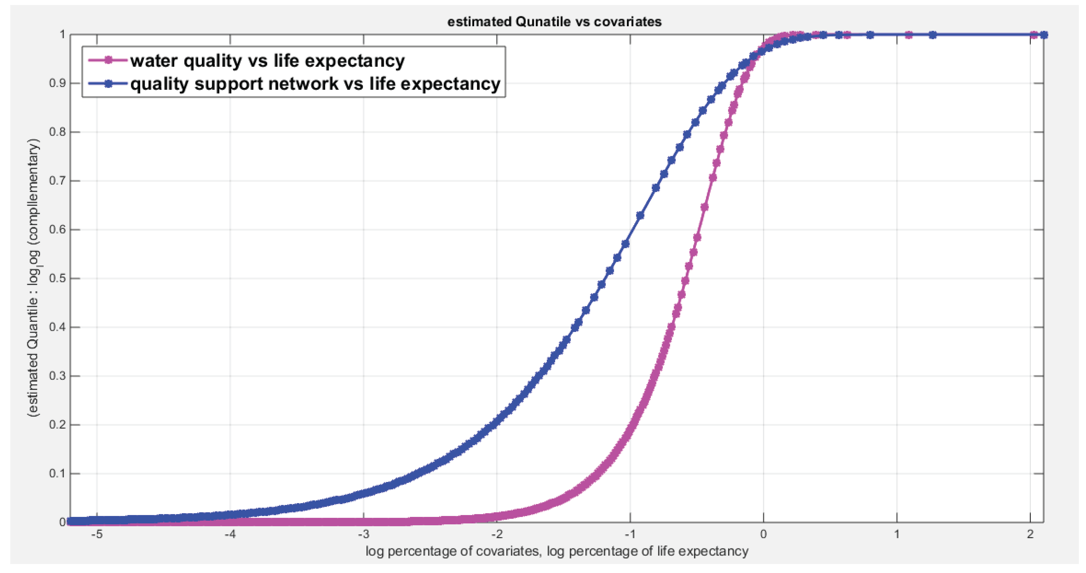
Figure 15.
Shows the QQ plot of the empirical vs. the theoretical quantiles for the log-log complementary model where the water quality is regressed on the life expectancy. The randomized quantile residuals show near perfect alignment all through the course of the curve in contrast to the Cox-Snell residuals which show more or less near alignment mainly in the lower tail and center of the curve than the upper tail.
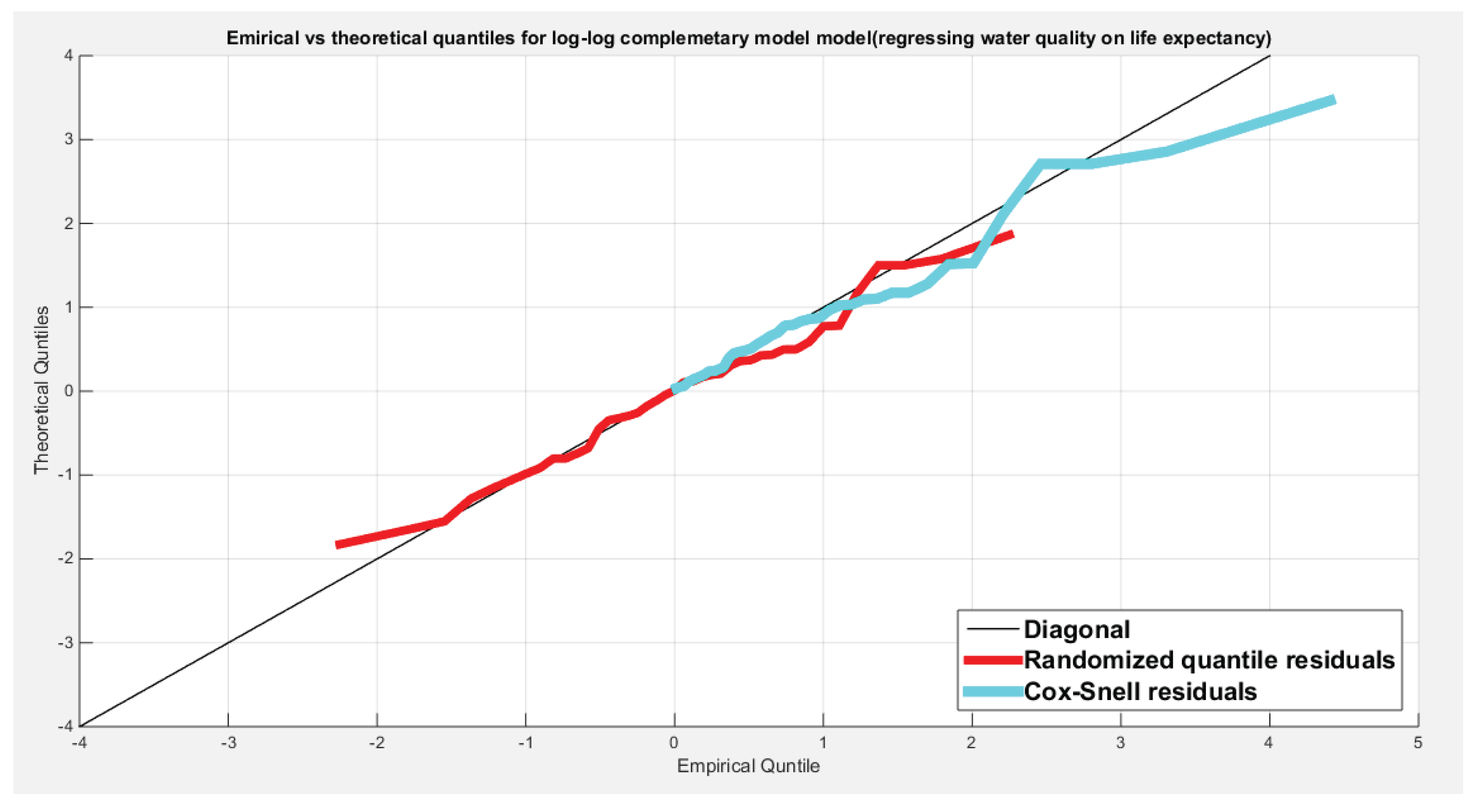
Figure 16.
Shows the QQ plot of the empirical vs. the theoretical quantiles for the log-log complementary model where the quality of support network is regressed on the life expectancy. The randomized quantile residuals show near perfect alignment all through the course of the curve in contrast to the Cox-Snell residuals which show more or less near alignment mainly in the lower tail and center of the curve than the upper tail.
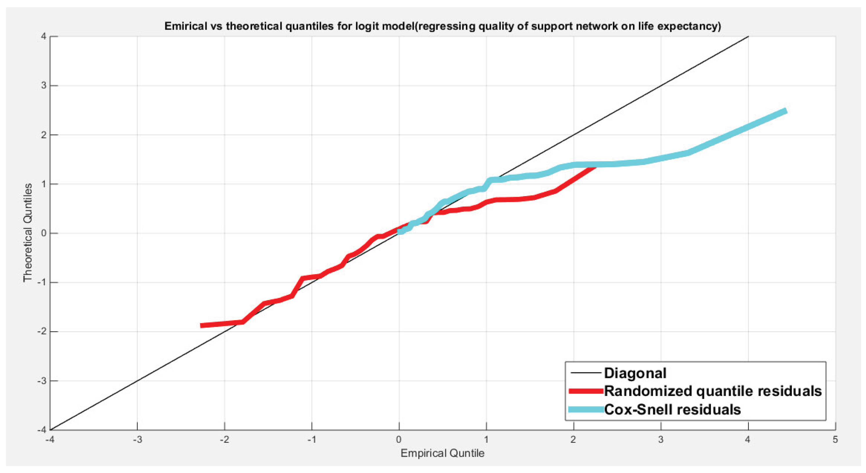
Figure 17.
Shows the scatter plot between the life expectancy predictor (transformed) and the randomized quantile residuals and Cox-Snell residuals for the log-log complementary model regressing the life expectancy on water quality. There is no specific trend or relationship between them and the scatter is random. No evidence of dependence between the predictor and the residuals of both types. The Kendall tau dependency parameter between the predictor and the residuals is -0.1093 with p-value= 0.3225 which is not statistically significant. These values are true for both types of residuals.
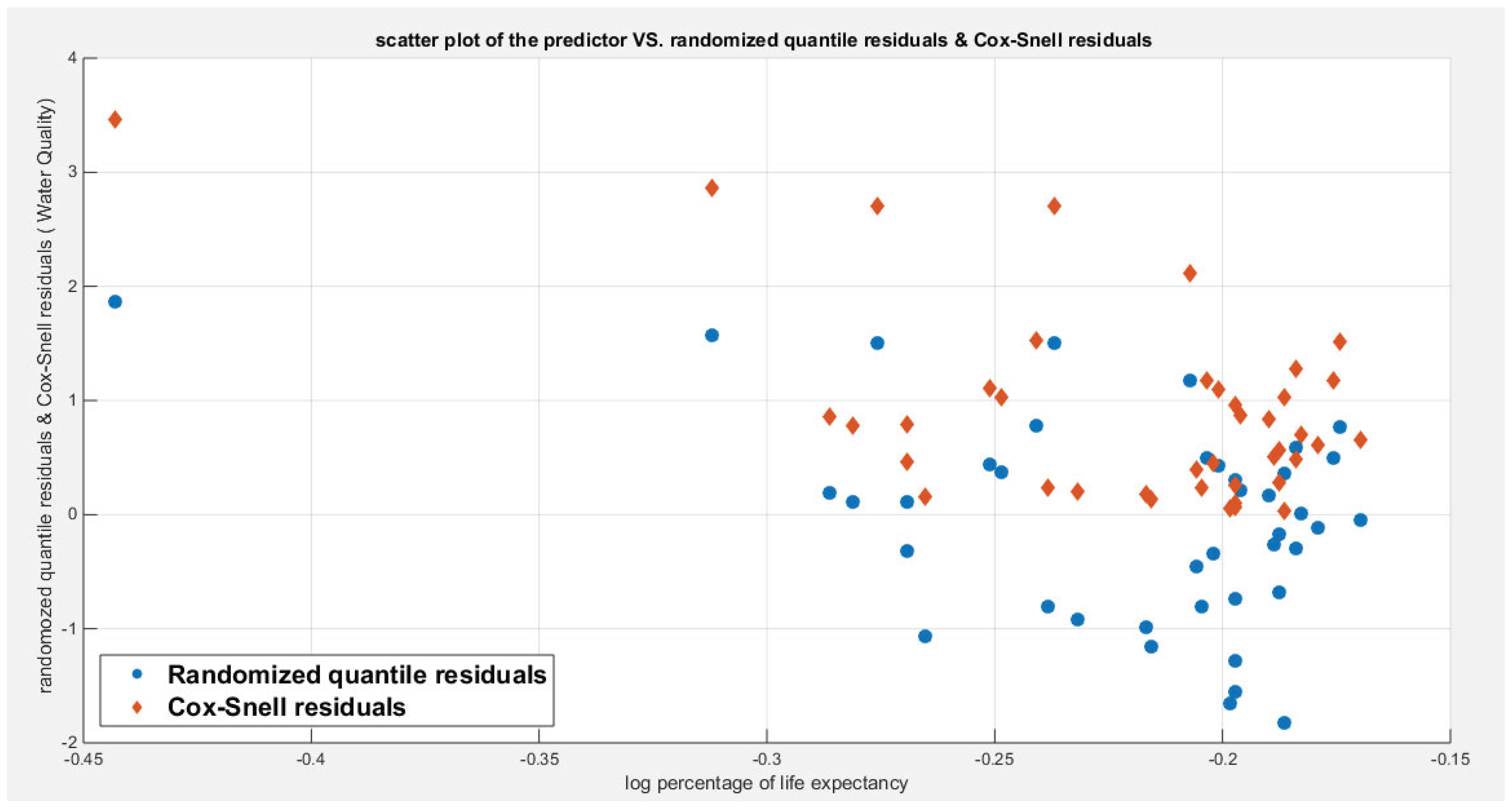
Figure 18.
Shows the scatter plot between the life expectancy predictor (transformed) and the randomized quantile residuals and Cox-Snell residuals for the log-log complementary model regressing the life expectancy on quality of support network. There is no specific trend or relationship between them and the scatter is random. No evidence of dependence between the predictor and the residuals of both types. The Kendall tau dependency parameter between the predictor and the residuals is -0.1104 with p-value= 0.3171 which is not statistically significant. These values are true for both types of residuals.
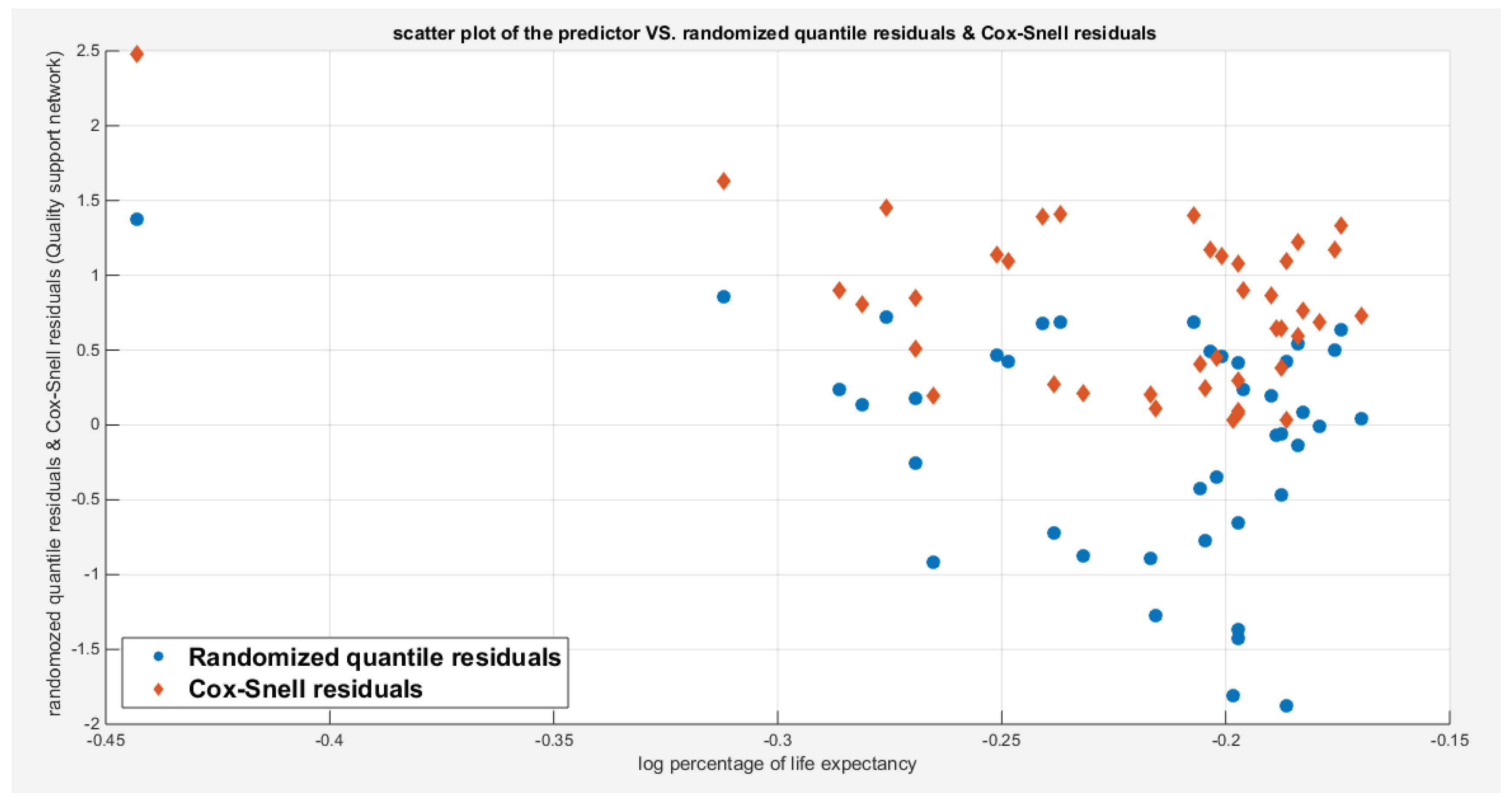
Figure 19.
Shows the parametric bootstrap sampling distribution of the CVM for the logit model depicting the significant of the CVM as the value 0.0032 lies between the 2.5th and the 97.5th quantile. .
Figure 19.
Shows the parametric bootstrap sampling distribution of the CVM for the logit model depicting the significant of the CVM as the value 0.0032 lies between the 2.5th and the 97.5th quantile. .
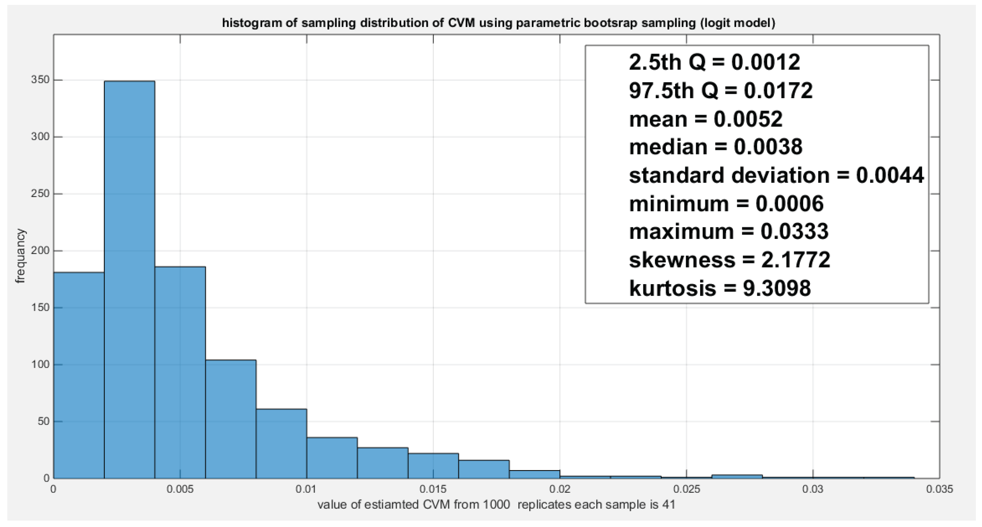
Figure 20.
Shows the parametric bootstrap sampling distribution of the intercept coefficient (g0) for the logit model depicting a non-significant coefficient as the zero value lies between the 2.5th and the 97.5th quantile. .
Figure 20.
Shows the parametric bootstrap sampling distribution of the intercept coefficient (g0) for the logit model depicting a non-significant coefficient as the zero value lies between the 2.5th and the 97.5th quantile. .
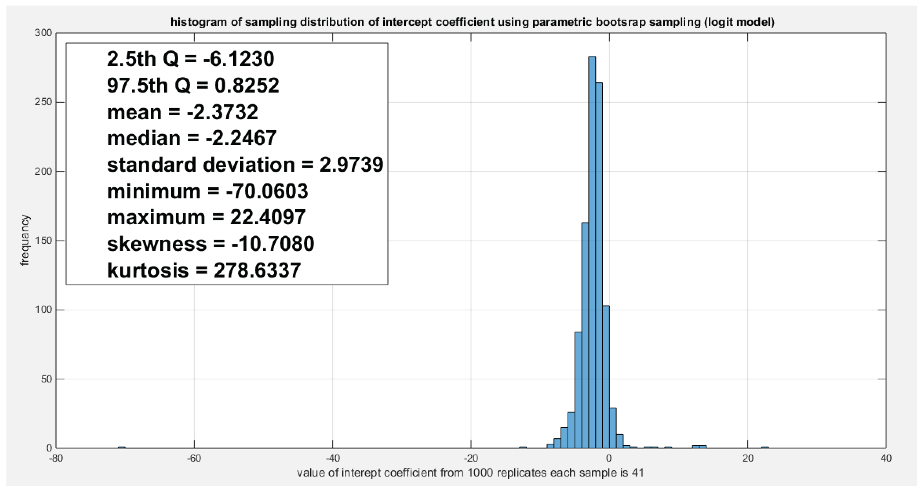
Figure 21.
Shows the parametric bootstrap sampling distribution of the slope coefficient (g1) for the logit model depicting the significance of the coefficient as the zero value do not lie between the 2.5th and the 97.5th quantile, and the estimated slope value (-14.6995) lies between these 2 quantiles. .
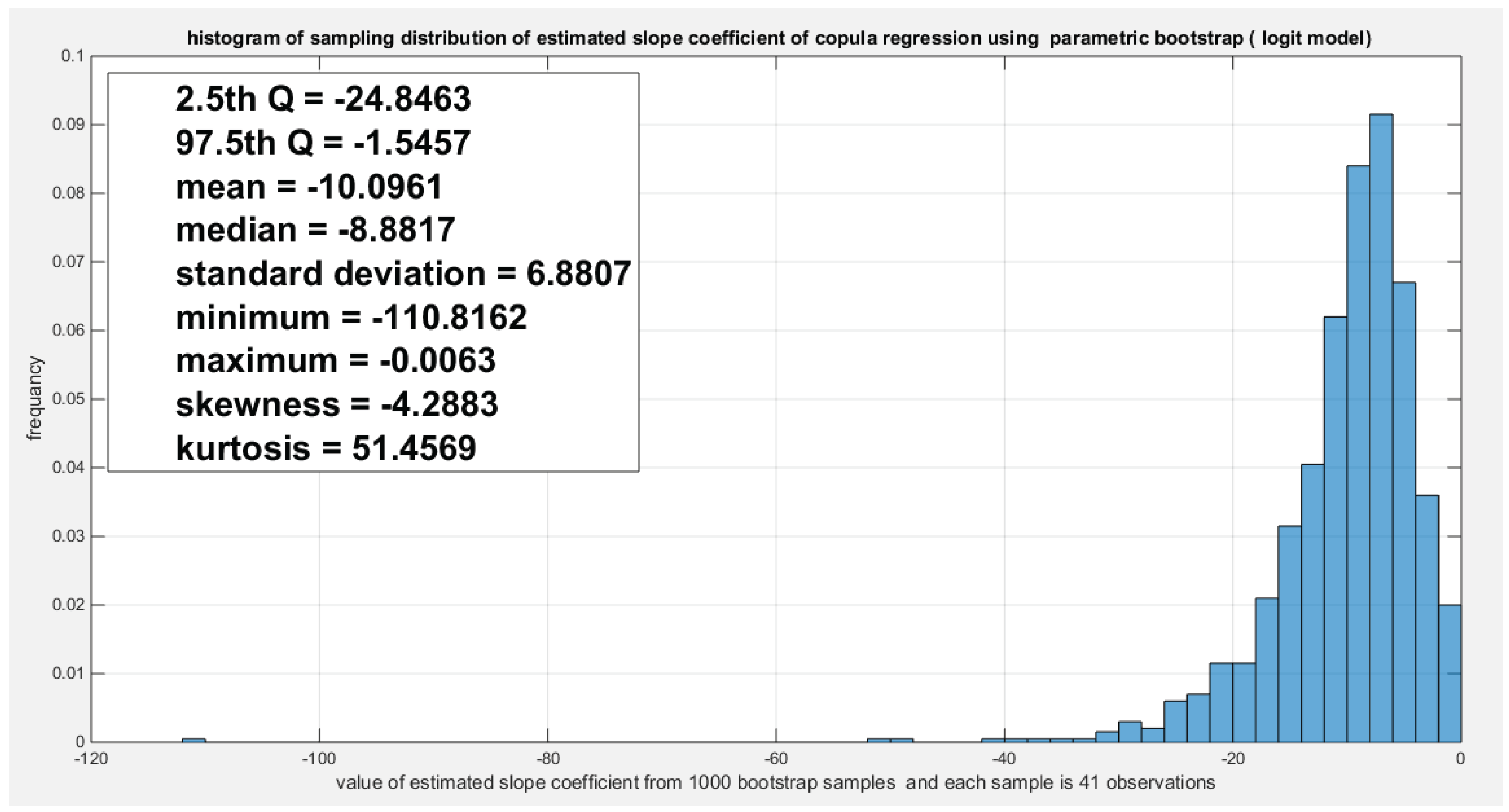
Figure 22.
Shows the parametric bootstrap sampling distribution of the LRT for the logit model depicting the significance of the ratio as the 4.3426 value does not lie between the 2.5th and the 97.5th quantile, it inhabits the upper tail.
Figure 22.
Shows the parametric bootstrap sampling distribution of the LRT for the logit model depicting the significance of the ratio as the 4.3426 value does not lie between the 2.5th and the 97.5th quantile, it inhabits the upper tail.
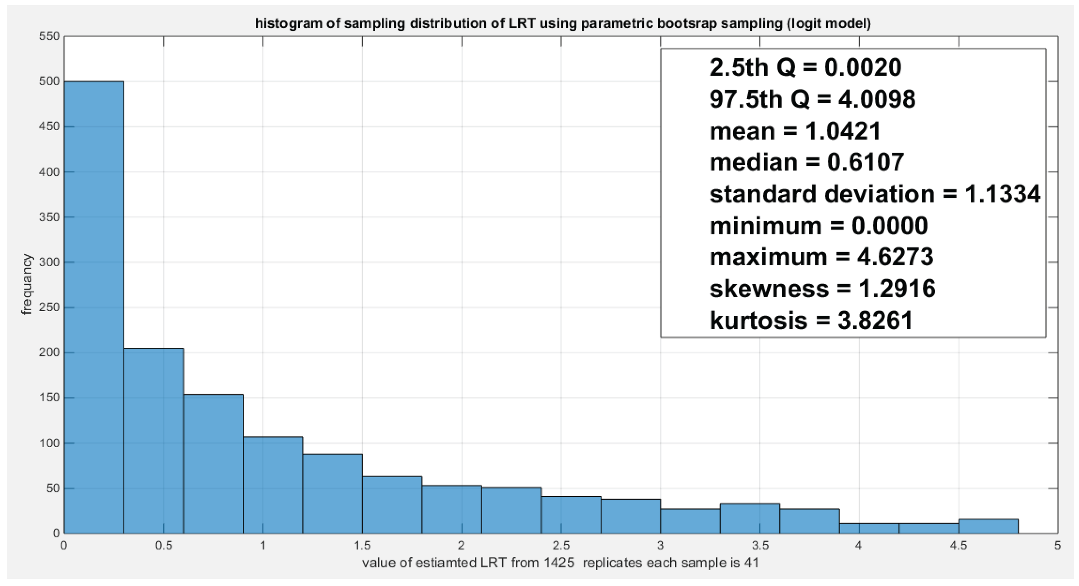
Figure 23.
Shows the parametric bootstrap sampling distribution of the CVM for the log-log complementary model depicting the significant of the CVM as the value 0.0033 lies between the 15th and the 85th quantile.
Figure 23.
Shows the parametric bootstrap sampling distribution of the CVM for the log-log complementary model depicting the significant of the CVM as the value 0.0033 lies between the 15th and the 85th quantile.
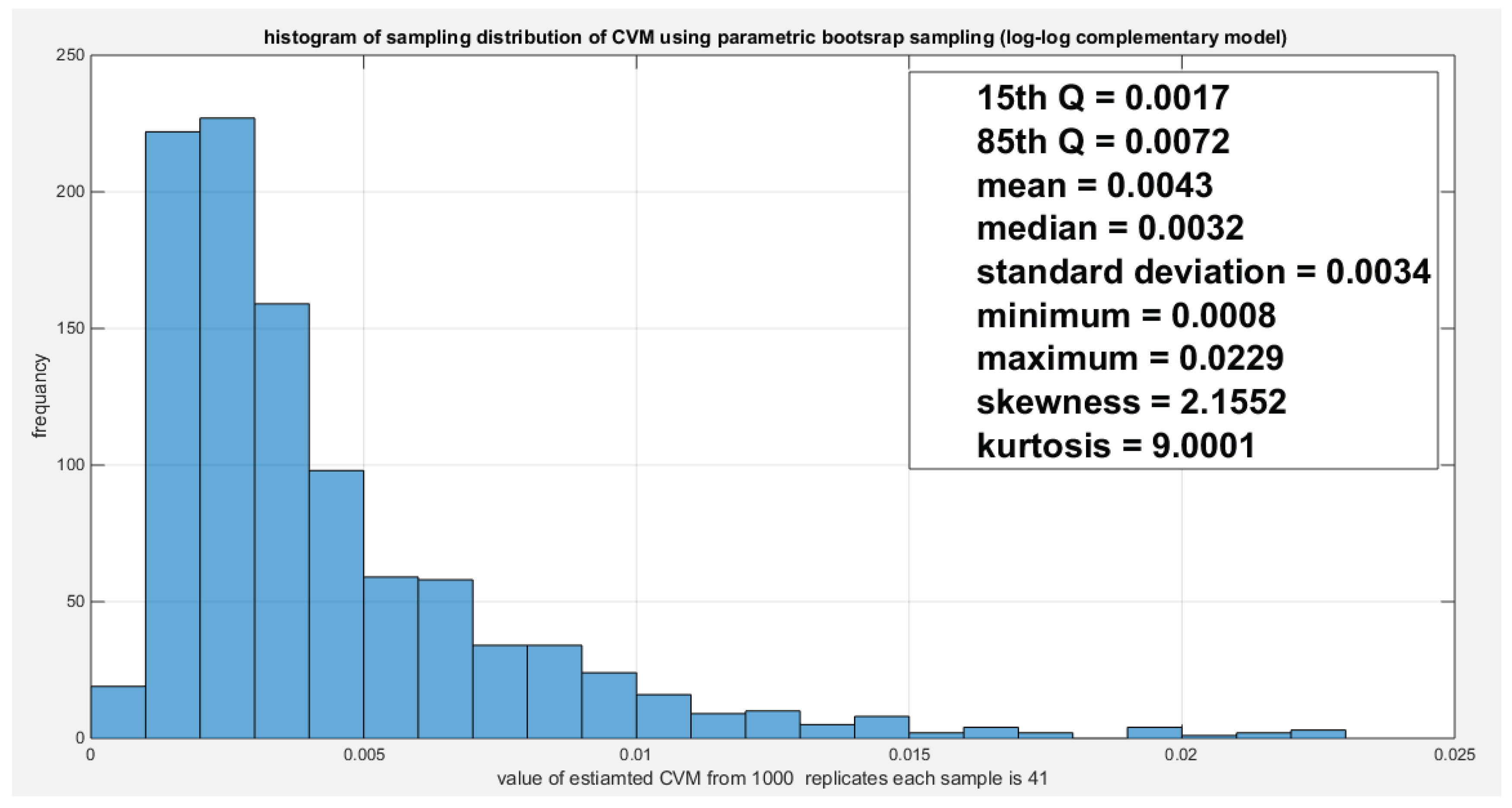
Figure 24.
Shows the parametric bootstrap sampling distribution of the intercept coefficient (g0) for the log-log complementary model depicting a non-significant coefficient as the zero value lies between the 15th and the 85th quantile. .
Figure 24.
Shows the parametric bootstrap sampling distribution of the intercept coefficient (g0) for the log-log complementary model depicting a non-significant coefficient as the zero value lies between the 15th and the 85th quantile. .
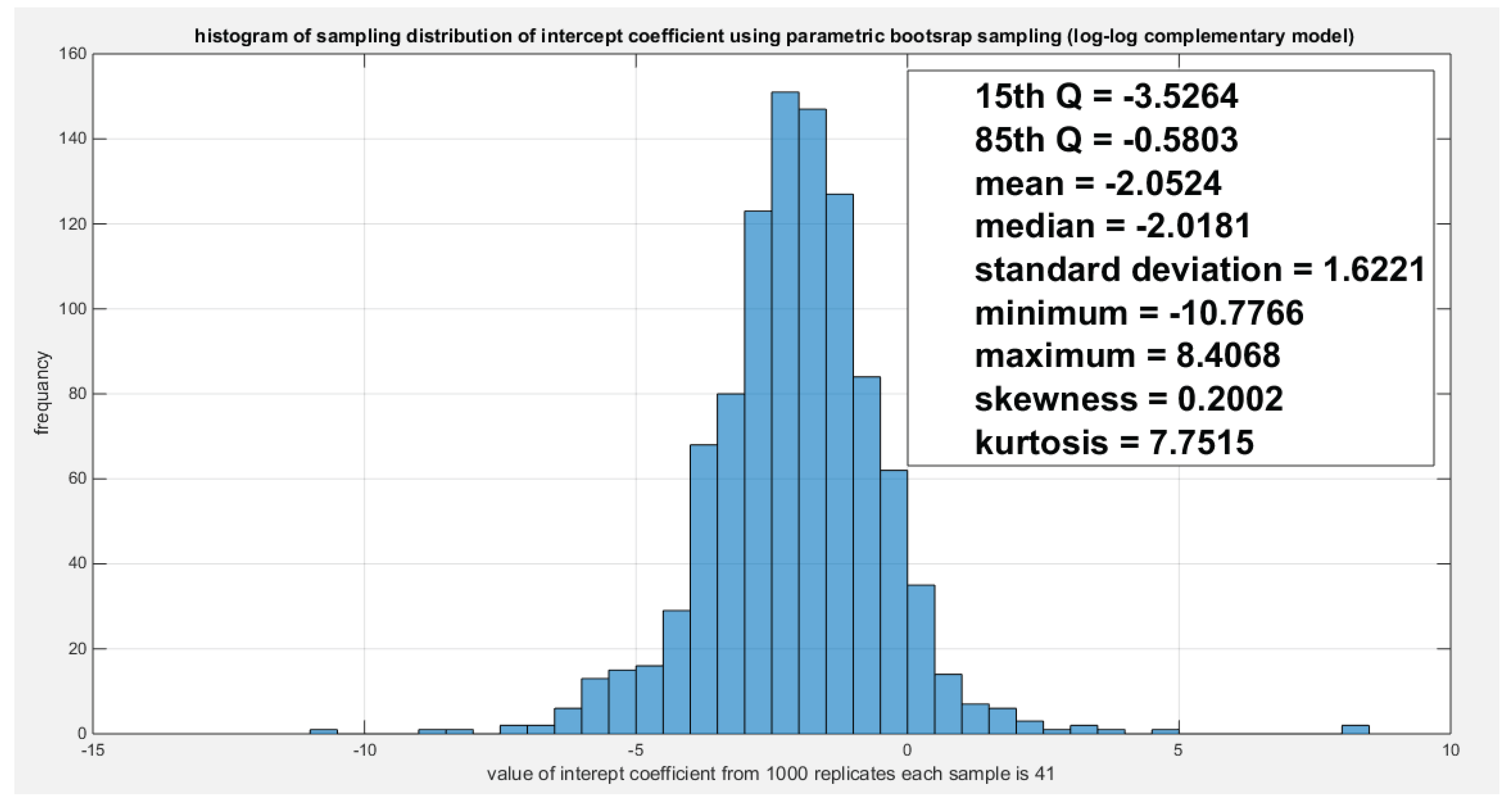
Figure 25.
Shows the parametric bootstrap sampling distribution of the slope coefficient (g1) for the log-log complementary model depicting the significance of the coefficient as the zero value do not lie between the 15th and the 85th quantile, and the estimated slope value (-12.6233) lies between these 2 quantiles.
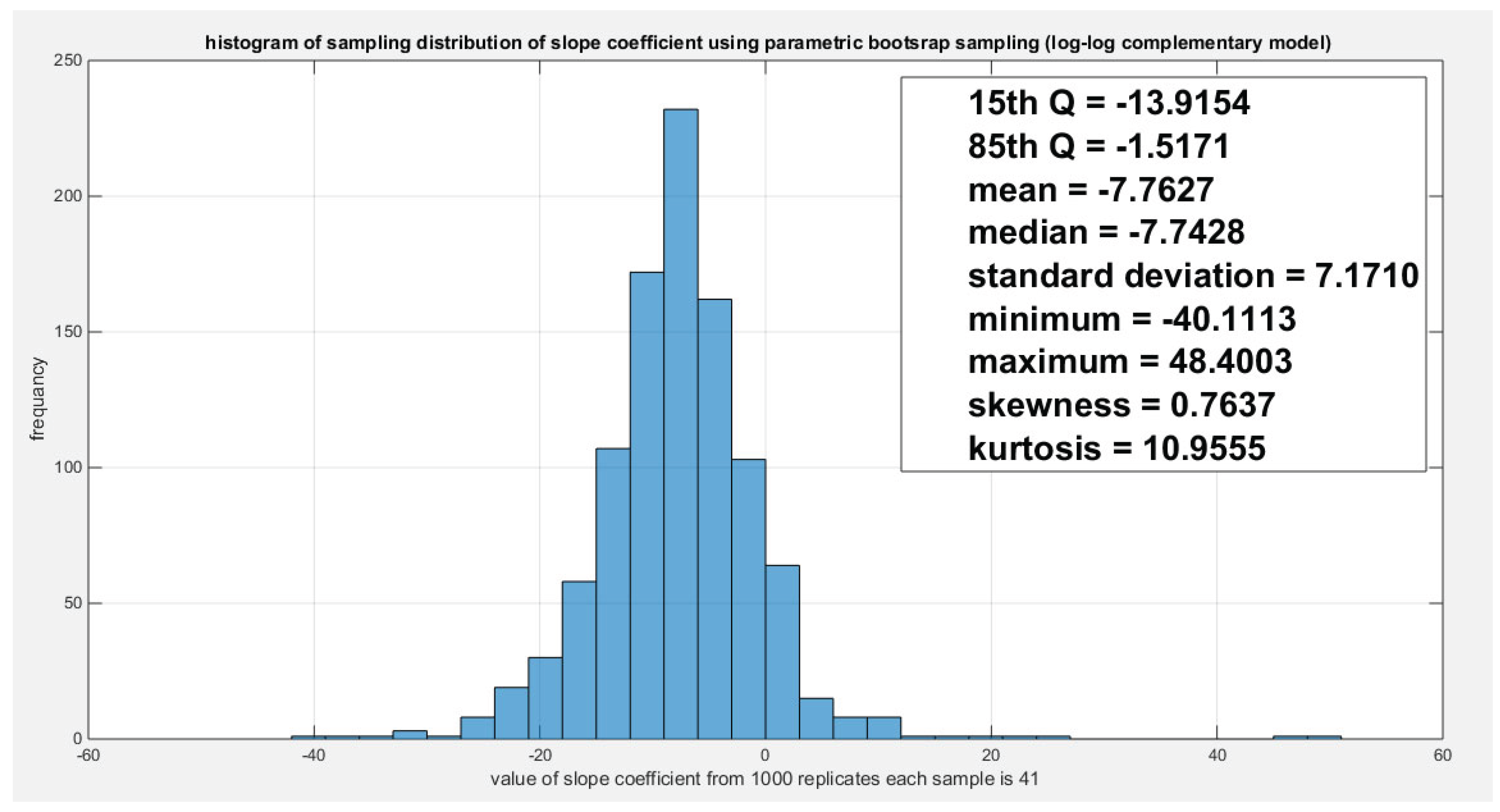
Figure 26.
Shows the parametric bootstrap sampling distribution of the CVM for the log-log complementary model depicting the significant of the CVM as the value 0.0033 lies between the 2.5th and the 97.5th quantile. .
Figure 26.
Shows the parametric bootstrap sampling distribution of the CVM for the log-log complementary model depicting the significant of the CVM as the value 0.0033 lies between the 2.5th and the 97.5th quantile. .
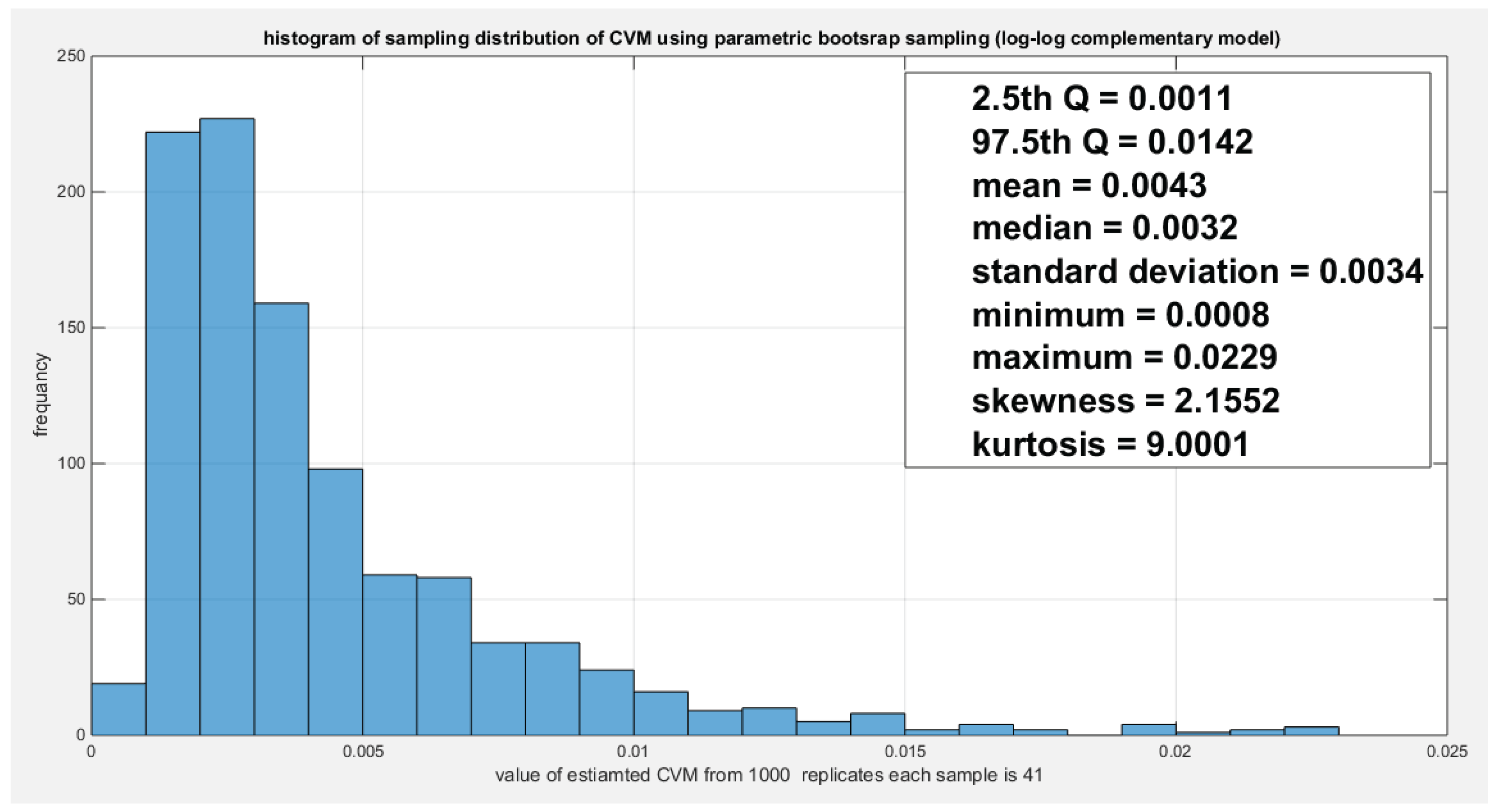
Figure 27.
Shows the non-parametric bootstrap sampling distribution of the slope coefficient (g1) for the log-log complementary model depicting the significance of the coefficient as the zero value do not lie between the 2.5th and the 97.5th quantile, and the estimated slope value (-12.6233) lies between these 2 quantiles. But this sampling is less powerful than the parametric bootstrap sampling.
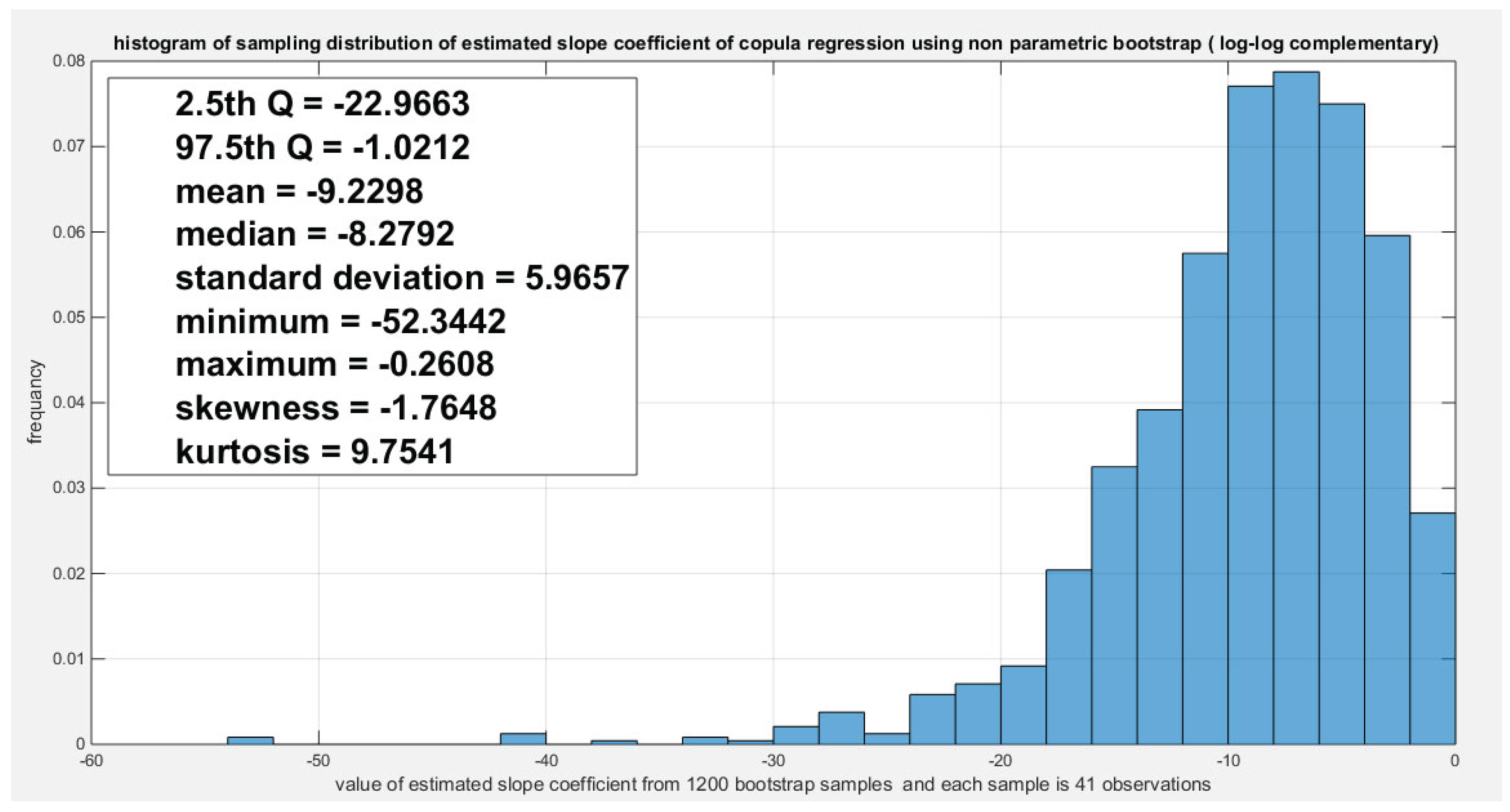
Figure 28.
Shows the parametric bootstrap sampling distribution of the LRT for the log-log complementary model depicting the significance of the ratio as the 3.8243 value does not lie between the 15th and the 85th quantile, it occupies the upper tail.
Figure 28.
Shows the parametric bootstrap sampling distribution of the LRT for the log-log complementary model depicting the significance of the ratio as the 3.8243 value does not lie between the 15th and the 85th quantile, it occupies the upper tail.
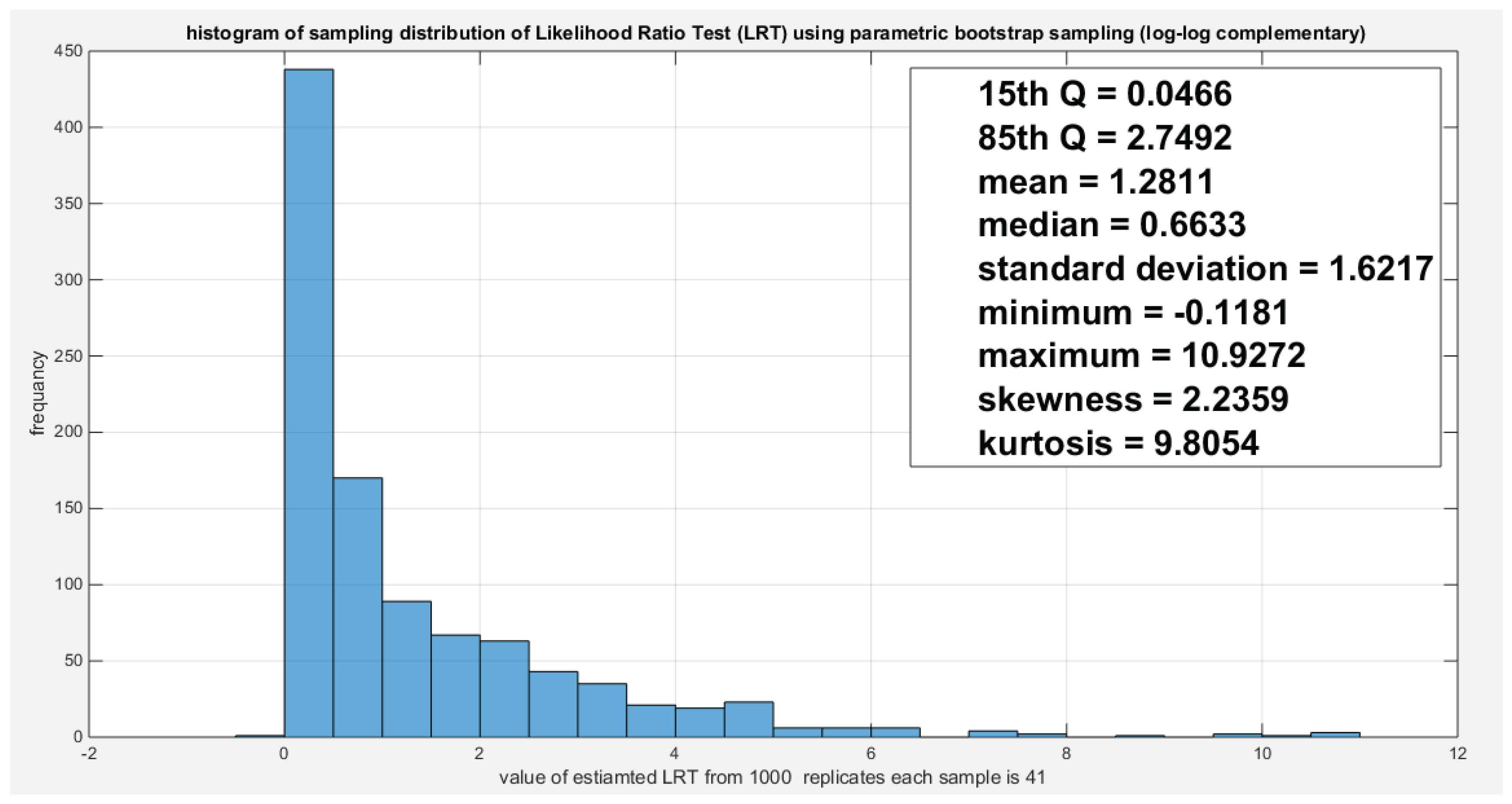
Figure 29.
Shows the estimated dependency parameter vs. the log percentage of the life expectancy for the logit model. As the life expectancy increase, the dependency between the 2 response variables weakens..
Figure 29.
Shows the estimated dependency parameter vs. the log percentage of the life expectancy for the logit model. As the life expectancy increase, the dependency between the 2 response variables weakens..
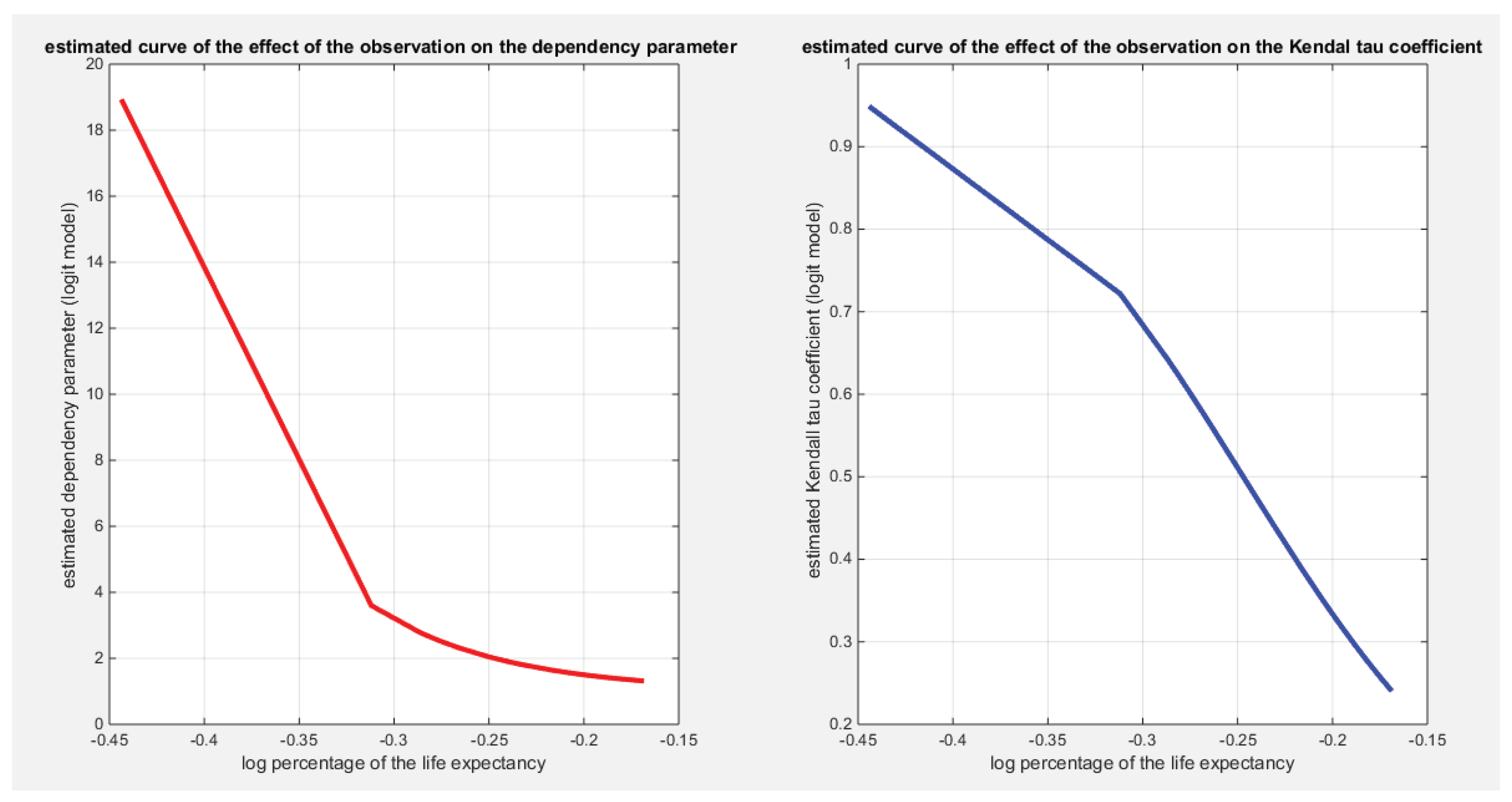
Figure 30.
Shows the estimated dependency parameter vs. the log percentage of the life expectancy for the log-log complementary model. The dependency between the 2 response variables weakens as the life expectancy increases.
Figure 30.
Shows the estimated dependency parameter vs. the log percentage of the life expectancy for the log-log complementary model. The dependency between the 2 response variables weakens as the life expectancy increases.
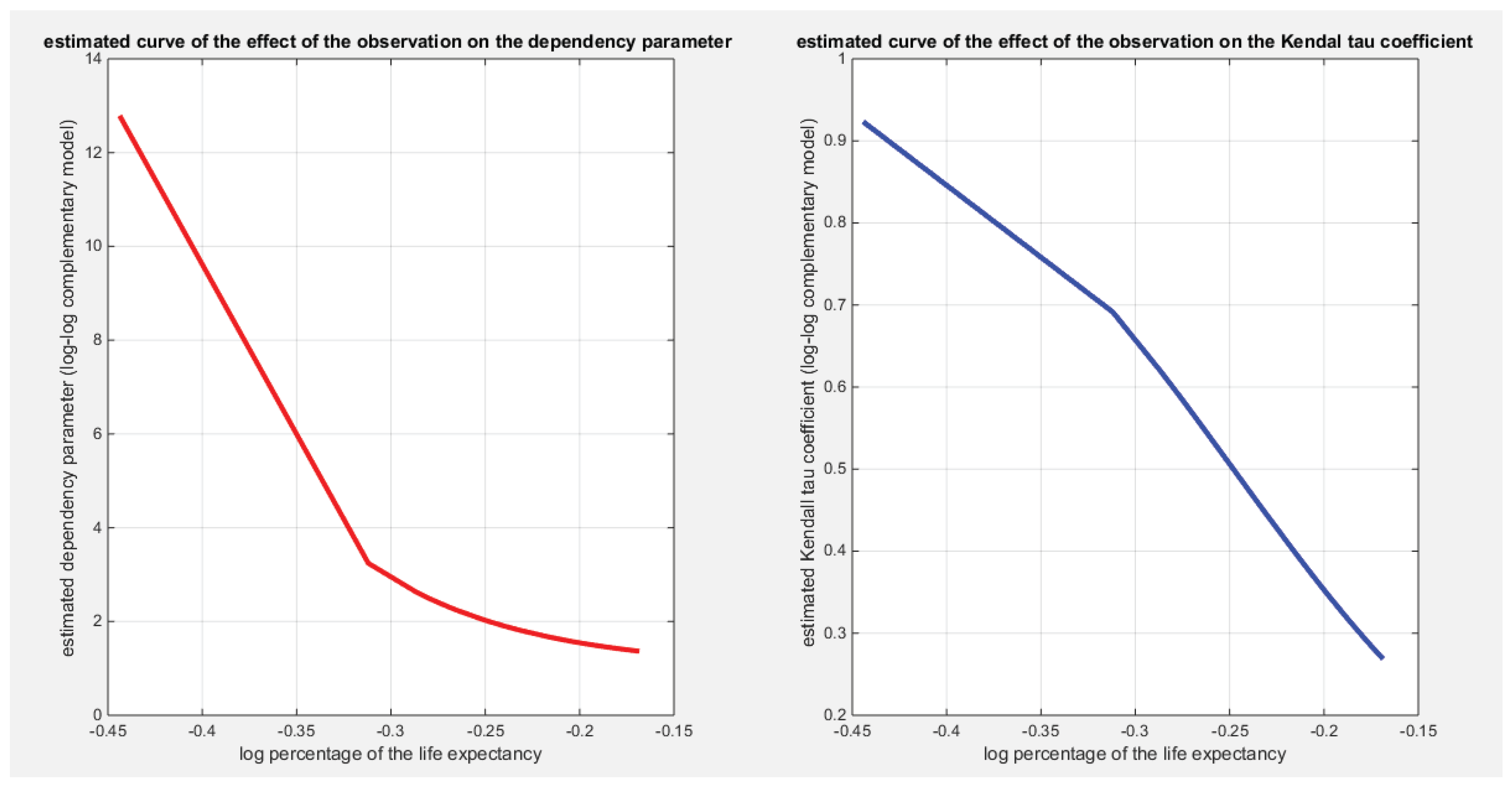
Figure 31.
Shows the empirical copula vs. the theoretical copula after applying step 4 of the algorithm using the u& v obtained from the logit regression model in step 3 of the algorithm.
Figure 31.
Shows the empirical copula vs. the theoretical copula after applying step 4 of the algorithm using the u& v obtained from the logit regression model in step 3 of the algorithm.
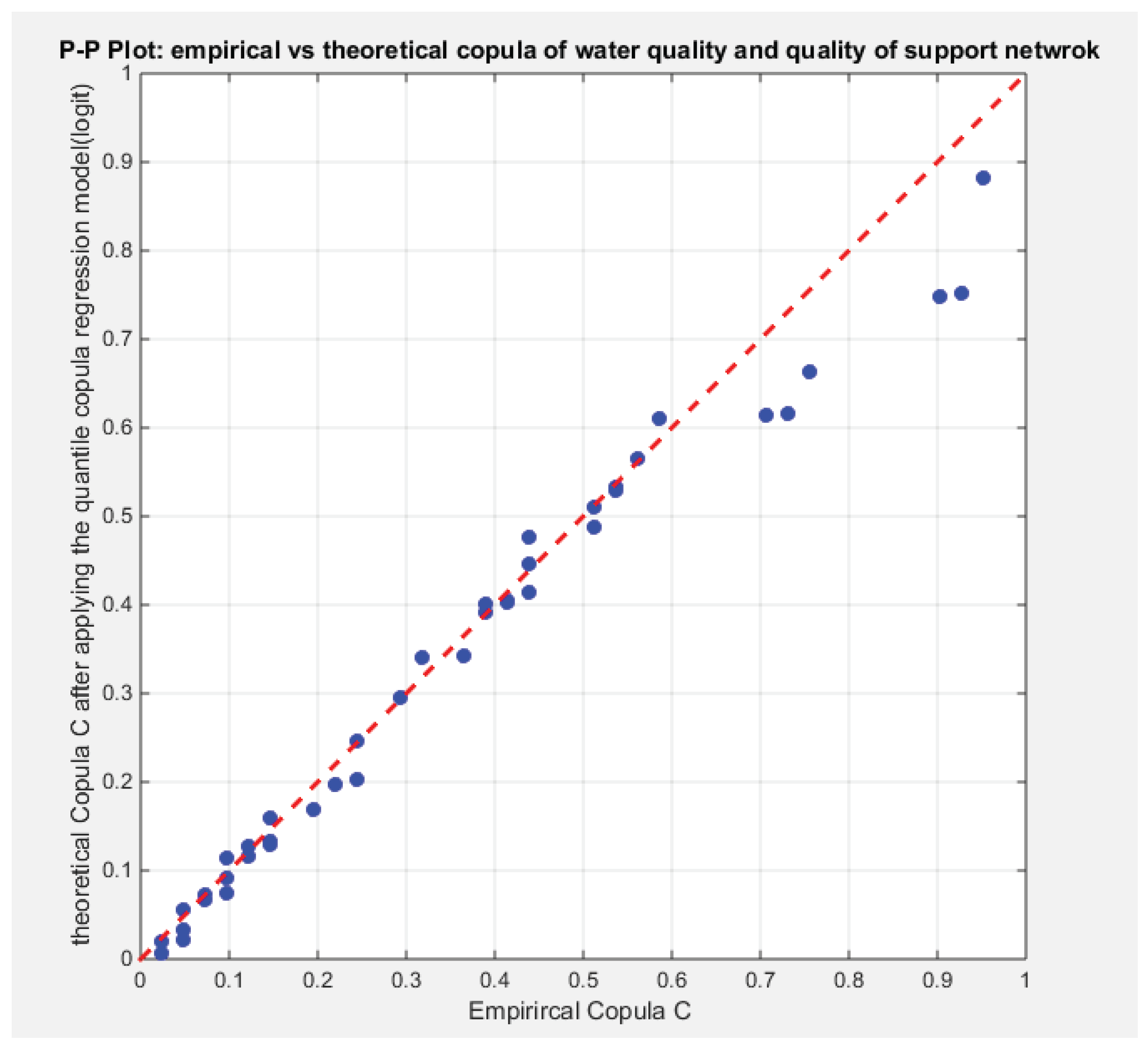
Figure 32.
Shows the empirical copula vs. the theoretical copula after applying step 4 of the algorithm using the u& v obtained from the log-log complementary regression model in step 3 of the algorithm.
Figure 32.
Shows the empirical copula vs. the theoretical copula after applying step 4 of the algorithm using the u& v obtained from the log-log complementary regression model in step 3 of the algorithm.
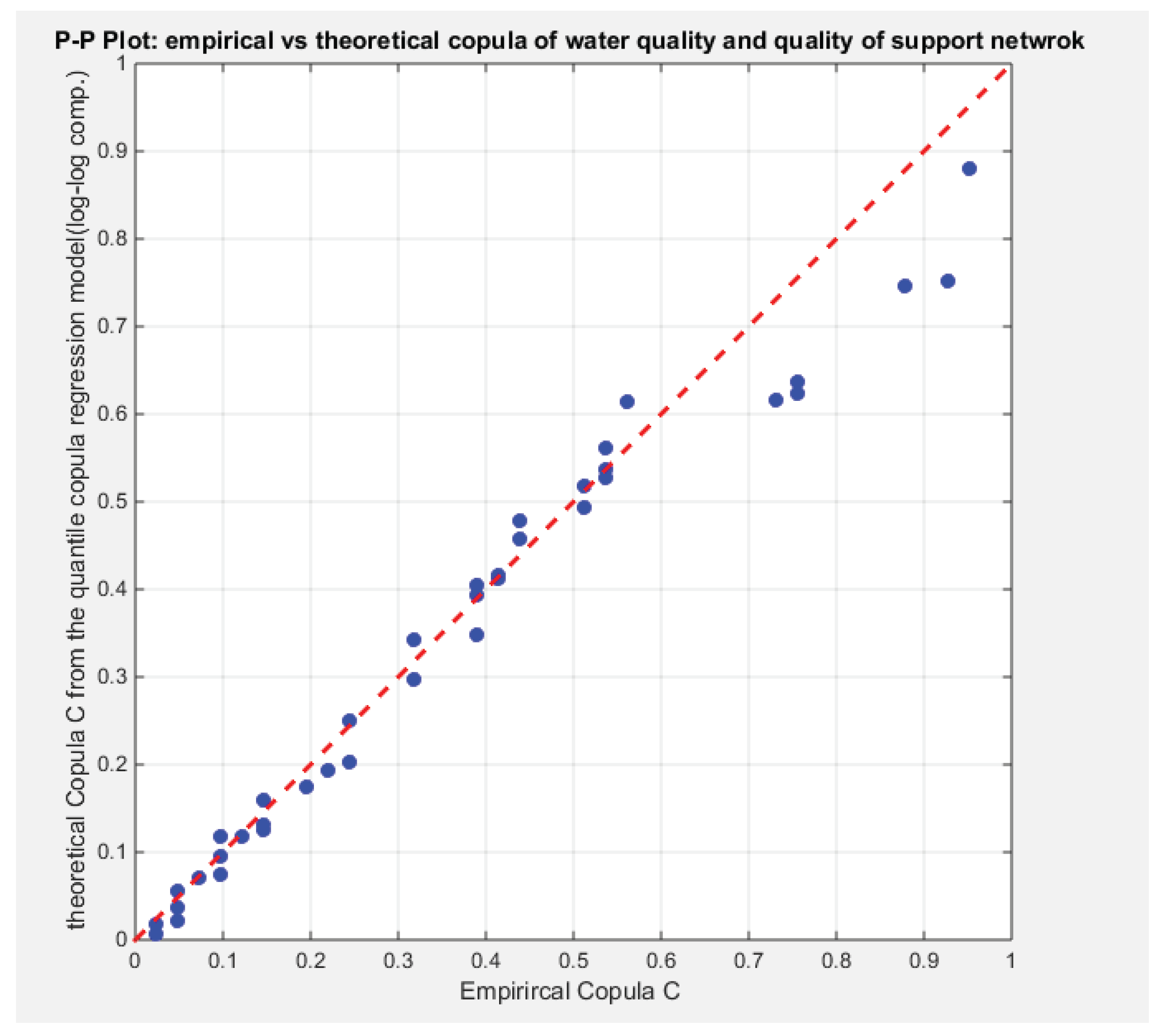

Table 1.
The descriptive statistics of the two response variables.
| indicator | min | mean | Standard deviation | skewness | kurtosis | 25percentile | 50percentile | 75percentile | max |
| Water quality | 0.62 | 0.8332 | 0.0972 | -0.6059 | 2.9144 | 0.7775 | 0.83 | 0.91 | 0.98 |
| Quality of support network | 0.77 | 0.9078 | 0.0538 | -1.176 | 3.5406 | 0.89 | 0.93 | 0.95 | 0.98 |
Table 2.
Kendall Tau coefficient between the two response variables.
| Water quality | Quality of support network | |
| Water quality | 1 |
0.3929 (0.0006) |
| Quality of support network |
0.3929 (0.0006) |
1 |
Table 3.
Statistical indices for the two response variables.
| indicator | Estimated theta | variance | AIC | CAIC | BIC | HQIC | KS-test | Ho | p-value of KS-test |
| Water quality | 0.4776 | 0.00072157 | -78.9952 | -78.8926 | -77.2817 | -78.3712 | 0.0991 | Fail to reject | 0.7789 |
| Quality of support network | 0.3444 | 0.00037494 | -131.651 | -131.6505 | -131.5479 | -131.0265 | 0.1806 | Fail to reject | 0.1217 |
Table 4.
The results of marginal regression of response variables on the predictor using the logit link function.
Table 4.
The results of marginal regression of response variables on the predictor using the logit link function.
| Regressing water quality on life expectancy using the logit link | Regressing quality of support network on life expectancy using the logit link | |||
| b0 | 3.0944 | 3.2216 | ||
| b1 | 5.8750 | 3.4077 | ||
| LL | 43.2027 | 67.7959 | ||
| Wald statistics of bo | 4.8932 (p-value <0.025) | 5.5193 (p-value <0.025) | ||
| Wald statistics of b1 | 2.0702 (p-value <0.025) | 1.3126 (p-value >0.025) | ||
| AIC | -82.4053 | -131.5917 | ||
| CAIC | -82.0896 | -131.2759 | ||
| BIC | -78.9782 | -128.1646 | ||
| HQIC | -81.1574 | -130.3437 | ||
| LRT ( likelihood Ratio Test) | 5.4102 (p-value=0.02) | 1.9412 ( p-value=0.1635) | ||
| p-value for the randomized quantile residual | 0.6821 | 0.1079 | ||
| p-value for the Cox-Snell residual | 0.6821 | 0.1079 | ||
| Variance-covariance matrix | 0.3999 | 1.7612 | 0.3407 | 1.4842 |
| 1.7612 | 8.0536 | 1.4842 | 6.7365 | |
Table 5.
The results of marginal regression of response variables on the predictor using the log-log link complementary function.
Table 5.
The results of marginal regression of response variables on the predictor using the log-log link complementary function.
| Regressing water quality on life expectancy using the log –log complementary link | Regressing quality of support network on life expectancy using the log-log complementary link | |||
| b0 | 1.2917 | 1.2317 | ||
| b1 | 2.848 | 1.3446 | ||
| LL | 43.3006 | 67.84 | ||
| Wald statistics of b0 | 4.282 (p-value<0.025) | 5.41 (p-value < 0.025) | ||
| Wald statistics of b1 | 2.0367 (p <0.025) | 1.297 (p-value > 0.025) | ||
| AIC | -82.6011 | -131.6799 | ||
| CAIC | -82.2853 | -131.3641 | ||
| BIC | -79.174 | -128.2528 | ||
| HQIC | -81.3532 | -130.4319 | ||
| LRT ( likelihood Ratio Test) | 5.6059 (p-value=0.0179) | 2.2094 ( p-value=0.1543) | ||
| p-value for the randomized quantile residual | 0.619 | 0.1033 | ||
| p-value for the Cox-Snell residual | 0.619 | 0.1033 | ||
| Variance-covariance matrix | 0.091 | 0.4154 | 0.0519 | 0.232 |
| 0.4154 | 1.9553 | 0.232 | 1.0732 | |
Table 6.
Shows the results utilizing the fitted CDFs (u & v) from model of regression, the logit model and the log-log complementary.
Table 6.
Shows the results utilizing the fitted CDFs (u & v) from model of regression, the logit model and the log-log complementary.
| after the log-log complementary regression model | after the logit regression model | |||
| g0 | -3.1311 | -3.6314 | ||
| g1 | -12.6233 | -14.6995 | ||
| LL | -70.8383 | -70.6029 | ||
| Wald statistics of g0 | 2.509(p-value <0.025) | 2.4176(p-value <0.025) | ||
| Wald statistics of g1 | 2.6713(p-value <0.025) | 2.58155(p-value <0.025) | ||
| AIC | 145.6766 | 145.2058 | ||
| CAIC | 145.9924 | 145.5216 | ||
| BIC | 149.1034 | 148.6329 | ||
| HQIC | 146.9246 | 146.4538 | ||
| CVM | 0.0033 | 0.0032 | ||
| Empirical tau, (P-value) | 0.3356 (0.0021) | 0.3331 (0.0025) | ||
| Mean of theoretical tau | 0.4147 | 0.4045 | ||
| LRT, (P-value) | 3.8243 (0.0505) | 4.3426 (0.0372) | ||
| Variance-covariance matrix | 1.5569 | 5.7163 | 2.2562 | 8.3667 |
| 5.7163 | 22.3305 | 8.3667 | 32.4221 | |
Disclaimer/Publisher’s Note: The statements, opinions and data contained in all publications are solely those of the individual author(s) and contributor(s) and not of MDPI and/or the editor(s). MDPI and/or the editor(s) disclaim responsibility for any injury to people or property resulting from any ideas, methods, instructions or products referred to in the content. |
© 2025 by the authors. Licensee MDPI, Basel, Switzerland. This article is an open access article distributed under the terms and conditions of the Creative Commons Attribution (CC BY) license (http://creativecommons.org/licenses/by/4.0/).
Copyright: This open access article is published under a Creative Commons CC BY 4.0 license, which permit the free download, distribution, and reuse, provided that the author and preprint are cited in any reuse.


