Choosing Between Link Functions for Median Parametric Regression Model Utilizing Median Base Unit Rayleigh Distribution

1.1. Logit Link Function

The response variable follows a MBUR distribution. To establish a causal relationship between this variable and the covariates that may be influencing it, it is crucial to properly specify both the parametric function and the link function. Given that the response variable may be highly skewed and could violate the assumptions of normality and homoscedasticity, using parametric quantile regression may offer a robust solution. However, it is important to explore all other potential techniques to achieve the best estimation results. The MBUR has the following PDF and CDF respectively as expressed in equations (1-2):

$$f\left(y\right)={\displaystyle \frac{6}{{\alpha }^2}}\left[1-y^{{\displaystyle \frac{1}{{\alpha }^2}}}\right]y^{\left({\displaystyle \frac{2}{{\alpha }^2}}-1\right)},0<y<1,\alpha >0$$

(1)

$$F\left(y\right)={3y}^{{\displaystyle \frac{2}{{\alpha }^2}}}-{2y}^{{\displaystyle \frac{3}{{\alpha }^2}}},0<y<1,\alpha >0$$

(2)

Quantile regression depends on the quantile function in equation (3):

$$y=F^{-1}\left(y\right)={\left\{-.5\left(cos\left[{\displaystyle \frac{{cos}^{-1}\left(1-2u\right)}{3}}\right]-\sqrt{3}sin\left[{\displaystyle \frac{{cos}^{-1}\left(1-2u\right)}{3}}\right]\right)+.5\right\}}^{{\alpha }^2}$$

(3)

Re-parameterize the PDF and CDF of MBUR using the quantile function , $y=c^{{\alpha }^2}$ , Where c is $c=-.5\left(cos\left[{\displaystyle \frac{{cos}^{-1}\left(1-2u\right)}{3}}\right]-\sqrt{3}sin\left[{\displaystyle \frac{{cos}^{-1}\left(1-2u\right)}{3}}\right]\right)+.5,u\in \left(\mathrm{0,1}\right).$U represents the chosen quantile, if it is the median, so u=.5 so ${\alpha }^2={\displaystyle \frac{ln\left(y\right)}{ln\left(c\right)}}$ . When replacing u=.5 in c, this gives $ln(.5)=-.6931$ , ${\alpha }^2={\displaystyle \frac{ln\left(y\right)}{ln\left(c\right)}}={\displaystyle \frac{ln\left(median\right)}{ln\left(c\right)}}$ . As y is the median corresponding to u=.5 .

Using the logit function of the median, which will be called $\mu$

$$Logit\left(median\right)=logit\left(\mu \right)=\phi =X^{\mathrm{\text{'}}}B={\beta }_0+{\beta }_1{x}_{i1}+\dots +{\beta }_k{x}_{ik};i=1,...,n\&k=1,\dots ,k$$

where n is the number of cases or observations and k is the number of variables. Logit median is the linear combination of variables.

So $\mu ={\displaystyle \frac{e^{X^{\mathrm{\text{'}}}B}}{1+e^{X^{\mathrm{\text{'}}}B}}}={\displaystyle \frac{e^{\phi }}{1+e^{\phi }}}$ and ${\alpha }^2={\displaystyle \frac{ln\left(y\right)}{ln\left(c\right)}}={\displaystyle \frac{ln\left(median\right)}{ln\left(c\right)}}={\displaystyle \frac{ln\left(\frac{e^{X^{\mathrm{\text{'}}}B}}{1+e^{X^{\mathrm{\text{'}}}B}}\right)}{ln\left(c\right)}}={\displaystyle \frac{ln\left(\frac{e^{\phi }}{1+e^{\phi }}\right)}{ln\left(c\right)}}$The reparameterized PDF is $f\left(y\right)={\displaystyle \frac{6ln\left(c\right)}{ln\left(\frac{e^{X^{\mathrm{\text{'}}}B}}{1+e^{X^{\mathrm{\text{'}}}B}}\right)}}\left[1-y^{{\displaystyle \frac{ln\left(c\right)}{ln\left(\frac{e^{X^{\mathrm{\text{'}}}B}}{1+e^{X^{\mathrm{\text{'}}}B}}\right)}}}\right]y^{{\displaystyle \frac{2ln\left(c\right)}{ln\left(\frac{e^{X^{\mathrm{\text{'}}}B}}{1+e^{X^{\mathrm{\text{'}}}B}}\right)}}-1},0<y<1,\alpha >0$The reparameterized CDF is $F\left(y\right)={3y}^{{\displaystyle \frac{2ln\left(c\right)}{ln\left(\frac{e^{X^{\mathrm{\text{'}}}B}}{1+e^{X^{\mathrm{\text{'}}}B}}\right)}}}-{2y}^{{\displaystyle \frac{3ln\left(c\right)}{ln\left(\frac{e^{X^{\mathrm{\text{'}}}B}}{1+e^{X^{\mathrm{\text{'}}}B}}\right)}}},0<y<1,\alpha >0$The reparameterized quantile is ${F^{-1}\left(y\right)=\left\{-.5\left(cos\left[{\displaystyle \frac{{cos}^{-1}\left(1-2u\right)}{3}}\right]-\sqrt{3}sin\left[{\displaystyle \frac{{cos}^{-1}\left(1-2u\right)}{3}}\right]\right)+.5\right\}}^{{\displaystyle \frac{ln\left(\frac{e^{\phi }}{1+e^{\phi }}\right)}{ln\left(c\right)}}}$

1.1.1. Estimation Using Log-Likelihood Function

Re-parameterize the PDF and subsequently the log-likelihood by replacing this ${\alpha }^2$ in the log-likelihood function to estimate the parameter using MLE as shown in equations (4-5):

$$l\left(\alpha \right)=nln\left(6\right)-nln\left({\alpha }^2\right)+\sum _{i=1}^{n}ln\left[1-y_i^{{\displaystyle \frac{1}{{\alpha }^2}}}\right]+\sum _{i=1}^n\left({\displaystyle \frac{2}{{\alpha }^2}}-1\right)ln\left(y_i\right)$$

(4)

$$l\left(\alpha \right)=nln\left(6\right)-nln\left({\displaystyle \frac{ln\left(\frac{e^{\phi }}{1+e^{\phi }}\right)}{ln\left(c\right)}}\right)+\sum _{i=1}^{n}ln\left[1-y_i^{{\displaystyle \frac{ln\left(c\right)}{ln\left(\frac{e^{\phi }}{1+e^{\phi }}\right)}}}\right]+\sum _{i=1}^n\left({\displaystyle \frac{2ln\left(c\right)}{ln\left(\frac{e^{\phi }}{1+e^{\phi }}\right)}}-1\right)ln\left(y_i\right)$$

(5)

$$l\left(\beta \right)=nln\left(6\right)-nln\left({\displaystyle \frac{ln\left(\frac{e^{X^{\mathrm{\text{'}}}B}}{1+e^{X^{\mathrm{\text{'}}}B}}\right)}{ln\left(c\right)}}\right)+\sum _{i=1}^{n}ln\left[1-y_i^{{\displaystyle \frac{ln\left(c\right)}{ln\left(\frac{e^{X^{\mathrm{\text{'}}}B}}{1+e^{X^{\mathrm{\text{'}}}B}}\right)}}}\right]+\sum _{i=1}^n\left({\displaystyle \frac{2ln\left(c\right)}{ln\left(\frac{e^{X^{\mathrm{\text{'}}}B}}{1+e^{X^{\mathrm{\text{'}}}B}}\right)}}-1\right)ln\left(y_i\right)$$

Next, apply the chain rule to differentiate the log-likelihood for estimating the regression coefficients. The log-likelihood is divided into 3 terms.

$$f_1\left(\beta \right)=ln\left({\displaystyle \frac{ln\left(\frac{e^{X^{\mathrm{\text{'}}}B}}{1+e^{X^{\mathrm{\text{'}}}B}}\right)}{ln\left(c\right)}}\right),f_2\left(\beta \right)=ln\left[1-y_i^{{\displaystyle \frac{ln\left(c\right)}{ln\left(\frac{e^{X^{\mathrm{\text{'}}}B}}{1+e^{X^{\mathrm{\text{'}}}B}}\right)}}}\right],f_3\left(\beta \right)=\left({\displaystyle \frac{2ln\left(c\right)}{ln\left(\frac{e^{X^{\mathrm{\text{'}}}B}}{1+e^{X^{\mathrm{\text{'}}}B}}\right)}}-1\right)ln\left(y_i\right)$$

Each one of the above terms will be differentiated with respect to each of the regression coefficients using the chain rule.

$${\displaystyle \frac{\partial l\left(\beta \right)}{\partial {\beta }_k}}={\displaystyle \frac{\partial l\left(\beta \right)}{\partial \mu }}{\displaystyle \frac{\partial \mu }{\partial \phi }}{\displaystyle \frac{\partial \phi }{\partial \beta }}$$

The linear regression equation with any number of variables can be expressed as

$logit\left(\mu \right)=\phi =X^{\mathrm{\text{'}}}B={\beta }_0+{\beta }_k{x}_{ik}$ and hence $\mu ={\displaystyle \frac{e^{\phi }}{1+e^{\phi }}}={\displaystyle \frac{e^{{\beta }_0+{\beta }_{ik}{x}_{ik}}}{1+e^{{\beta }_0+{\beta }_{ik}{x}_{ik}}}}$Start with: differentiate the first term w.r.t. to both regression coefficients in equations (6)

$${\displaystyle \frac{{\partial f}_1\left(\beta \right)}{\partial {\beta }_0}}={\displaystyle \frac{\frac{\partial }{\partial \beta }\left(\frac{ln\left(\frac{e^{X^{\mathrm{\text{'}}}B}}{1+e^{X^{\mathrm{\text{'}}}B}}\right)}{ln\left(c\right)}\right)}{\frac{ln\left(\frac{e^{X^{\mathrm{\text{'}}}B}}{1+e^{X^{\mathrm{\text{'}}}B}}\right)}{ln\left(c\right)}}}={\displaystyle \frac{1}{\left(1+e^{\phi }\right)ln\left(\mu \right)}}\&{\displaystyle \frac{{\partial f}_1\left(\beta \right)}{\partial {\beta }_k}}={\displaystyle \frac{x_{ik}}{\left(1+e^{\phi }\right)ln\left(\mu \right)}}$$

(6)

Next, differentiate the second term w.r.t. to both regression coefficients in equations (7)

$${{\displaystyle \frac{\partial }{\partial {\beta }_0}}f}_2\left(\beta \right)={\displaystyle \frac{\partial }{\partial {\beta }_0}}ln\left[1-y_i^{{\displaystyle \frac{ln\left(c\right)}{ln\left(\frac{e^{X^{\mathrm{\text{'}}}B}}{1+e^{X^{\mathrm{\text{'}}}B}}\right)}}}\right]={\displaystyle \frac{\partial }{\partial {\beta }_0}}ln\left[1-y_i^{{\displaystyle \frac{ln\left(c\right)}{ln\left(\mu \right)}}}\right]$$

(7)

$${\displaystyle \frac{\partial f_2\left(\beta \right)}{\partial {\beta }_0}}={\displaystyle \frac{{-y}_i^{\frac{ln\left(c\right)}{ln\left(\mu \right)}}\left[ln\left(y\right)\right]\left[\frac{-ln\left(c\right)}{\left(1+e^{\phi }\right){\left[ln\left(\mu \right)\right]}^2}\right]}{\left[1-y_i^{\frac{ln\left(c\right)}{ln\left(\mu \right)}}\right]}}\&{\displaystyle \frac{\partial f_2\left(\beta \right)}{\partial {\beta }_k}}={\displaystyle \frac{{-y}_i^{\frac{ln\left(c\right)}{ln\left(\mu \right)}}\left[ln\left(y\right)\right]\left[\frac{-x_{ik1}ln\left(c\right)}{\left(1+e^{\phi }\right){\left[ln\left(\mu \right)\right]}^2}\right]}{\left[1-y_i^{\frac{ln\left(c\right)}{ln\left(\mu \right)}}\right]}}$$

Lastly, differentiate the third term w.r.t. to both regression coefficients

$${\displaystyle \frac{{\partial f}_3\left(\beta \right)}{\partial {\beta }_0}}={\displaystyle \frac{\partial }{\partial {\beta }_0}}\left({\displaystyle \frac{2ln\left(c\right)}{ln\left(\frac{e^{X^{\mathrm{\text{'}}}B}}{1+e^{X^{\mathrm{\text{'}}}B}}\right)}}-1\right)\ln y_i={\displaystyle \frac{-2ln\left(c\right)\ln y_i}{\left(1+e^{\phi }\right){\left[ln\left(\mu \right)\right]}^2}}\&{\displaystyle \frac{{\partial f}_3\left(\beta \right)}{\partial {\beta }_k}}={\displaystyle \frac{-2x_{ik}ln\left(c\right)\ln y_i}{\left(1+e^{\phi }\right){\left[ln\left(\mu \right)\right]}^2}}$$

These equations can be solved using numerical algorithm and an optimizer like the quas-newton:

$${\displaystyle \frac{\partial l\left(\beta \right)}{\partial {\beta }_0}}={\displaystyle \frac{-1}{\left(1+e^{\phi }\right)ln\left(\mu \right)}}+{\displaystyle \frac{{-y}_i^{\frac{ln\left(c\right)}{ln\left(\mu \right)}}\left[ln\left(y\right)\right]\left[\frac{-ln\left(c\right)}{\left(1+e^{\phi }\right){\left[ln\left(\mu \right)\right]}^2}\right]}{\left[1-y_i^{\frac{ln\left(c\right)}{ln\left(\mu \right)}}\right]}}+{\displaystyle \frac{-2ln\left(c\right)ln\left(y_i\right)}{\left(1+e^{\phi }\right){\left[ln\left(\mu \right)\right]}^2}}$$

$${\displaystyle \frac{\partial l\left(\beta \right)}{\partial {\beta }_k}}={\displaystyle \frac{-x_{ik}}{\left(1+e^{\phi }\right)ln\left(\mu \right)}}+{\displaystyle \frac{{-y}_i^{\frac{ln\left(c\right)}{ln\left(\mu \right)}}\left[ln\left(y_i\right)\right]\left[\frac{-x_{ik}ln\left(c\right)}{\left(1+e^{\phi }\right){\left[ln\left(\mu \right)\right]}^2}\right]}{\left[1-y_i^{\frac{ln\left(c\right)}{ln\left(\mu \right)}}\right]}}+{\displaystyle \frac{-2x_{ik}ln\left(c\right)ln\left(y_i\right)}{\left(1+e^{\phi }\right){\left[ln\left(\mu \right)\right]}^2}}$$

Where i=1,2,…,n and k=1,2,..,p the n are the number of observations while the k are the number of parmaeters or predictors.

1.2. Log-Log Median Link Function

A link function other than the logit can be used. The author used the log-log function

$\log \left\{-\log \left(median\right)\right\}=X^{\mathrm{\text{'}}}B=\phi ={\beta }_0+{\beta }_1{x}_{i1}+\dots +{\beta }_k{x}_{ik},i=\mathrm{1,2},\dots ..,n\&k=\mathrm{1,2},\dots ..,k$$median=e^{-e^{X\mathrm{\text{'}}\beta }}=exp\left(-exp\left(X^{\mathrm{\text{'}}}\beta \right)\right)\&{\alpha }^2={\displaystyle \frac{ln\left(median\right)}{ln\left(c\right)}}={\alpha }^2={\displaystyle \frac{ln\left(e^{-e^{X\mathrm{\text{'}}\beta }}\right)}{ln\left(c\right)}}={\displaystyle \frac{-e^{X^{\mathrm{\text{'}}}\beta }}{ln\left(c\right)}}$Now using this parameter to re-parameterize the log-likelihood and the following functions

The reparameterized PDF is $f\left(y\right)={\displaystyle \frac{6}{\frac{-e^{X^{\mathrm{\text{'}}}\beta }}{ln\left(c\right)}}}\left[1-y^{{\displaystyle \frac{1}{\frac{-e^{X^{\mathrm{\text{'}}}\beta }}{ln\left(c\right)}}}}\right]y^{{\displaystyle \frac{2}{\frac{-e^{X^{\mathrm{\text{'}}}\beta }}{ln\left(c\right)}}}-1},0<y<1,\alpha >0$The reparameterized CDF is $F\left(y\right)={3y}^{{\displaystyle \frac{2}{\left(\frac{-e^{X^{\mathrm{\text{'}}}B}}{\ln c}\right)}}}-{2y}^{{\displaystyle \frac{3}{\left(\frac{-e^{X^{\mathrm{\text{'}}}B}}{\ln c}\right)}}},0<y<1,\alpha >0$The reparameterized quantile is: ${F^{-1}\left(y\right)=\left\{-.5\left(cos\left[{\displaystyle \frac{{cos}^{-1}\left(1-2u\right)}{3}}\right]-\sqrt{3}sin\left[{\displaystyle \frac{{cos}^{-1}\left(1-2u\right)}{3}}\right]\right)+.5\right\}}^{{\displaystyle \frac{-e^{X^{\mathrm{\text{'}}}\beta }}{ln\left(c\right)}}}$And for this link function the derivatives of the reparameterized log-likelihood function are:

$${\displaystyle \frac{\partial l\left(\beta \right)}{\partial {\beta }_0}}=-1+{\displaystyle \frac{{-y}_i^{\frac{ln\left(c\right)}{-e^{\phi }}}\left[ln\left(y\right)\right]\left[ln\left(c\right)\right]\left[e^{-\phi }\right]\left(1\right)}{\left[1-y_i^{\frac{ln\left(c\right)}{-e^{\phi }}}\right]}}+2ln\left(c\right)ln\left(y_i\right)\left[e^{-\phi }\right]\left(1\right)$$

$${\displaystyle \frac{\partial l\left(\beta \right)}{\partial {\beta }_k}}=-x_{ik}+{\displaystyle \frac{{-y}_i^{\frac{ln\left(c\right)}{-e^{\phi }}}\left[ln\left(y\right)\right]\left[ln\left(c\right)\right]\left[e^{-\phi }\right]\left(x_{ik}\right)}{\left[1-y_i^{\frac{ln\left(c\right)}{-e^{\phi }}}\right]}}+2ln\left(c\right)ln\left(y_i\right)\left[e^{-\phi }\right]x_{ik}$$

1.3. Complementary Log-Log Link Function

$\log \left\{-\log \left(1-median\right)\right\}=X^{\mathrm{\text{'}}}B=\phi ={\beta }_0+{\beta }_1{x}_{i1}+\dots +{\beta }_k{x}_{ik};i=1,..,n\&k=1,..,k$$median=1-e^{-e^{X^{\mathrm{\text{'}}}\beta }}=1-exp\left(-exp\left(X^{\mathrm{\text{'}}}\beta \right)\right)\&{\alpha }^2={\displaystyle \frac{ln\left(median\right)}{ln\left(c\right)}}={\displaystyle \frac{ln\left(1-e^{-e^{\phi }}\right)}{ln\left(c\right)}}$And for this link function the derivatives of the reparameterized log-likelihood function are:

$${\displaystyle \frac{\partial l\left(\beta \right)}{\partial {\beta }_0}}={\displaystyle \frac{{-e}^{-e^{\phi }}{e}^{\phi }}{\ln \mu }}+{\displaystyle \frac{y_i^{\frac{ln\left(c\right)}{\ln \mu }}\left[ln\left(y\right)\right]\left[ln\left(c\right)\right]\left[e^{-e^{\phi }}{e}^{\phi }\right]}{\left[1-y_i^{\frac{ln\left(c\right)}{\ln \mu }}\right]\left[\mu \right]\left[\ln \mu \right]}}-{\displaystyle \frac{2ln\left(c\right)ln\left(y_i\right)\left[e^{-e^{\phi }}{e}^{\phi }\right]}{\mu \left[\ln \mu \right]}}$$

$${\displaystyle \frac{\partial l\left(\beta \right)}{\partial {\beta }_k}}={\displaystyle \frac{{{-x}_{ik}e}^{-e^{\phi }}{e}^{\phi }}{\ln \mu }}+{\displaystyle \frac{y_i^{\frac{ln\left(c\right)}{\ln \mu }}\left[ln\left(y\right)\right]\left[ln\left(c\right)\right]\left[e^{-e^{\phi }}{e}^{\phi }\right]\left(x_{ik}\right)}{\left[1-y_i^{\frac{ln\left(c\right)}{\ln \mu }}\right]\left[\mu \right]\left[\ln \mu \right]}}-{\displaystyle \frac{2ln\left(c\right)ln\left(y_i\right)\left[e^{-e^{\phi }}{e}^{\phi }\right]\left(x_{ik}\right)}{\mu \left[\ln \mu \right]}}$$

2.1. Goodness of Fit Measures

Model adequacy can be evaluated by analyzing the residuals. In quantile regression, two well-known types of residuals are examined for their distribution.

First type: Randomized quantile (RQ) residuals: ${\mathit{r}}_{\mathit{i}}^{\mathit{R}\mathit{Q}}={\mathsf{\Phi }}^{-1}\left(\mathit{F}\left({\mathit{y}}_{\mathit{i}},\widehat{\mathit{\beta }}\right)\right)$$\mathsf{\Phi }$ is the standard normal CDF. F is the re-parameterized MBUR CDF given in equation (6). $y_i$ are the observations and $\widehat{\beta }$ are the estimated regression coefficients. These residuals are approximately distributed as standard normal. When the model is correctly specified, these residuals approximately follow the standard normal distribution.

Second type: Cox-Snell (CS) residuals: ${\mathit{r}}_{\mathit{i}}^{\mathit{C}\mathit{S}}=-\mathit{l}\mathit{o}\mathit{g}\left(1-\mathit{F}\left({\mathit{y}}_{\mathit{i}},\widehat{\mathit{\beta }}\right)\right)$Cox-Snell residuals are approximately distributed as a standard exponential distribution with a scale parameter of one. The negative logarithm mentioned above represents the cumulative distribution function (CDF) of the standard exponential distribution with this scale parameter. When the model is correctly specified, these residuals will approximately follow a standard exponential distribution.

2.2. Model Selection Criteria

Models are selected based on the lowest values of AIC, BIC, and Corrected AIC among the available options. (Sánchez, Leiva, Saulo, et al., 2021) used the $R_M^2$ , which is correspondent to the usual $R^2$ in mean regression. So it can be used and it is defined as

$$R_M^2=1-exp\left({\displaystyle \frac{2}{n}}\left(l\left(\check{\theta }\right)-l\left(\widehat{\theta }\right)\right)\right)$$

where $l\left(\check{\theta }\right)andl\left(\widehat{\theta }\right)$ are the maximum log-likelihood for the model without covariates (null model) and the model with all covariates (Full model).

$AIC=-2l\left(\widehat{\theta }\right)+2p$, $CAIC=AIC+{\displaystyle \frac{2p\left(p+1\right)}{n-p-1}}$, $BIC=-2l\left(\widehat{\theta }\right)+p\log \left(n\right)$where p is the number of parameters and n is the sample size.

3.1. Descriptive Analysis

Table 1 shows the dataset obtained from the OECD which stands for Organization for Economic Co-operation and Development. MATLAB was used for analysis. Nealder Mead optimizer was used to estimate the parameters. Finite central difference method was used to calculate the variance.

The data is available at https://stats.oecd.org/index.aspx?DataSetCode=BLI

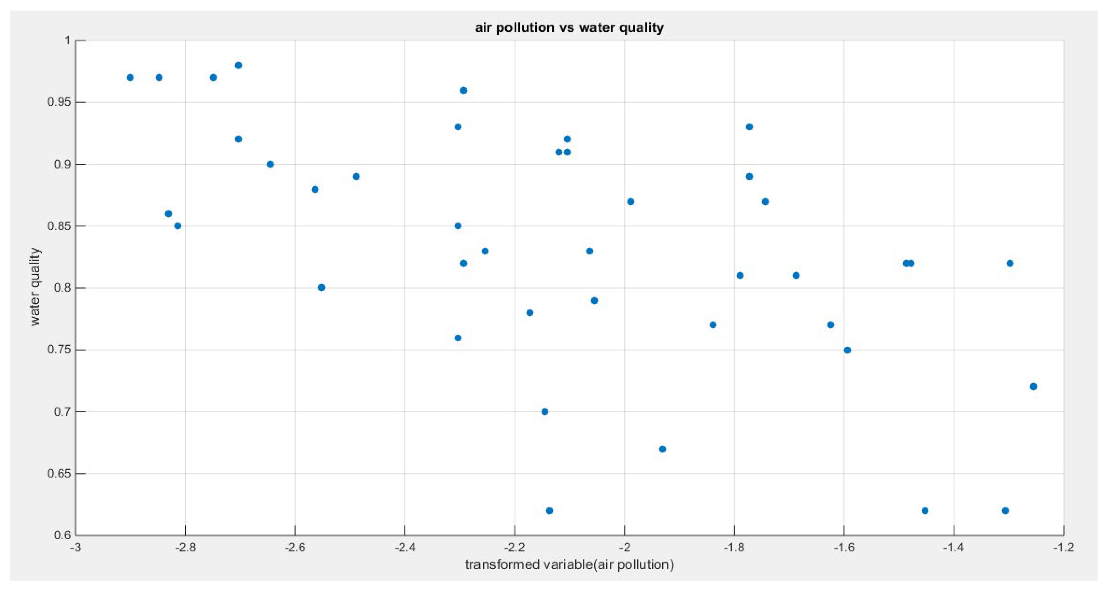
The water quality indicator is expressed as the percentage of population satisfied with the water quality. The air pollution is the expressed as the concentration of PM2.5 in the air and is measured in micrograms per cubic meter. Higher concentration indicates worse air quality.

Water quality data values are: 0.92, 0.92, 0.79, 0.9, 0.62, 0.82, 0.87, 0.89, 0.93, 0.86, 0.97, 0.78, 0.91, 0.67, 0.81, 0.97, 0.8, 0.77, 0.77, 0.87, 0.82, 0.83, 0.83, 0.85, 0.75, 0.91, 0.85, 0.98, 0.82, 0.89, 0.81, 0.93, 0.76, 0.97, 0.96, 0.62, 0.82, 0.88, 0.7, 0.62, 0.72. the descriptive statistics of this dataset are; the mean is 0.8332, the standard deviation is 0.0972, the skewness is -0.6059, the kurtosis is 2.9144, the minimum value is 0.62, the maximum value is 0.98, the 25th quantile is 0.7775, the median is 0.83, and the 75th quantile is 0.91. The data are negatively skewed (left skewness) and platykurtic.

Air pollution data values are: 6.7, 12.2, 12.8, 7.1, 23.4, 22.6, 17.5, 17, 10, 5.9, 5.5, 11.4, 12, 14.5, 16.7, 6.4, 7.8, 19.7, 15.9, 13.7, 27.3, 12.7, 10.5, 10, 20.3, 12.2, 6, 6.7, 22.8, 8.3, 18.5, 17, 10, 5.8, 10.1, 27.1, 10.1, 7.7, 11.7, 11.8, 28.5. The descriptive statistics of the air pollution data are as follows; the mean is 13.5098, the standard deviation is 6.3942, the skewness is 0.8055, the kurtosis is 2.8203, minimum value is 5.5, the maximum value is 28.5, the 25th quantile is 8.175, the median is 12, and the 75th quantile is 17.125. The data are positively skewed (right skewness) and leptokurtic.

3.2. The Model: Regressing Water Quality on Air Pollution

The predictors are transformed by dividing the predictor by 100 and then taking the log of the result. The Kendall tau between the response variable and the predictor is -0.4144 and it is statistically significant with p value 1.783e-4. The response variable is distributed as Median Based Unit Rayleigh. The author used 3 models, in each model a different link function is utilized and the model is named after the name of the link function. The link functions are: the logit, the log-log, and the clog-log. The parameter is reparametrized and hence the PDF using different link functions. Each model results into estimated median value as well as estimated alpha parameter value for each observation. For each model there is a set of figures illustrating the fitted median vs. the predictors, the predictor against the residuals, the QQ plot for the randomized quantile residuals and the Cox-Snell residuals. Table 1 shows the comparison between the different models according to the link function. For each model, the estimated intercept and slope are recorded. The Wald statistics and the associated p value, the log-likelihood, AIC, CAIC, BIC, and HQIC are recorded. The Likelihood Ratio Test (LRT) and the associated p value are also reported. The R-squred is also shown. The Kendall tau with it p value reflecting the relation between the transformed predictors and the residuals are stated. The standard error can be determined by taking the square root of the diagonal of the variance-covariance matrix which is prescribed in the table.

Figure 1. Shows the scatter plot of the water quality against the transformed predictor (air pollution).

Figure 1. Shows the scatter plot of the water quality against the transformed predictor (air pollution).

Figures for the Logit Model

Figure 2. Shows the decreasing estimated curve for the median against the transformed predictor.

Figure 2. Shows the decreasing estimated curve for the median against the transformed predictor.

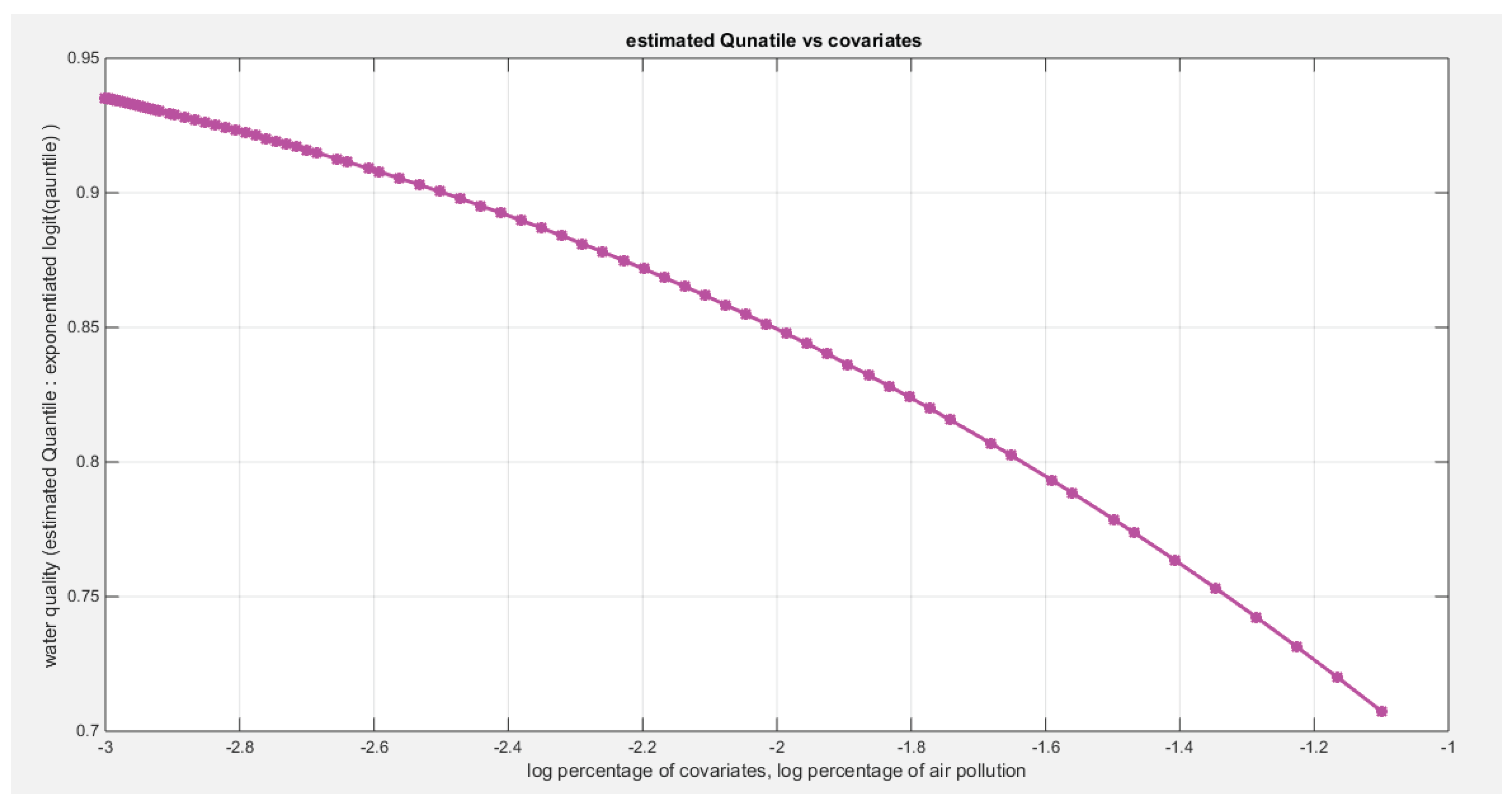
Figure 3. Shows the predictors vs. the residuals of both types. Both curves show no specific trend and they are randomly related.

Figure 3. Shows the predictors vs. the residuals of both types. Both curves show no specific trend and they are randomly related.

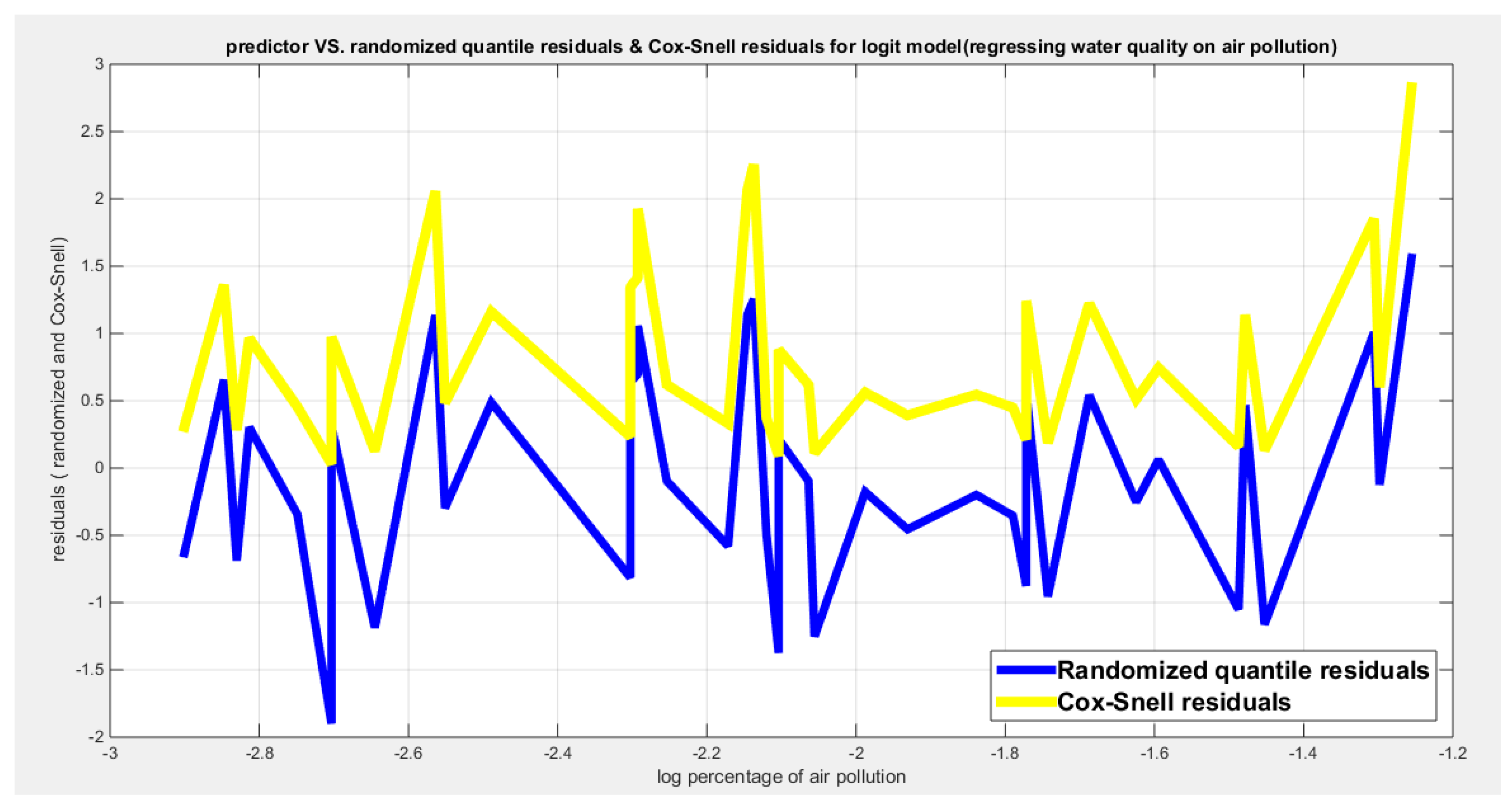
Figure 4. Shows the residuals against the predictors. No specific trend is there and they are randomly scattered. This behavior is clear and obvious for both types of residuals.

Figure 4. Shows the residuals against the predictors. No specific trend is there and they are randomly scattered. This behavior is clear and obvious for both types of residuals.

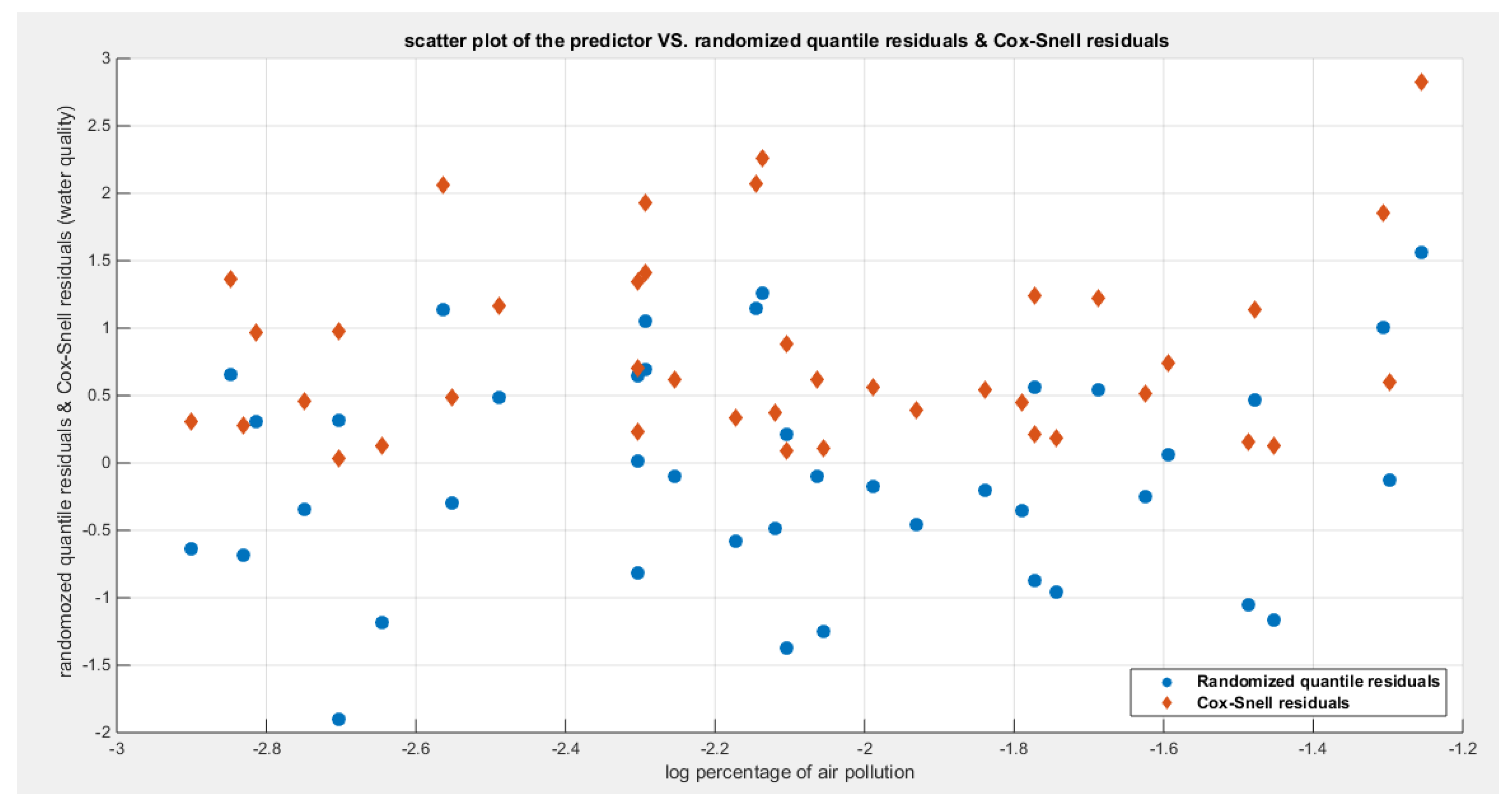
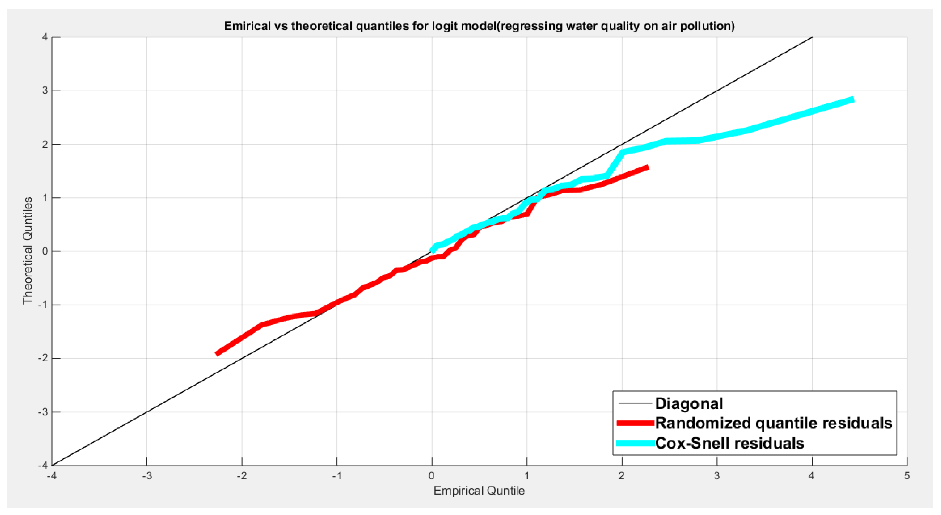
Figure 5. Shows the QQ plot of the empirical quantiles for both residuals . The randomized quantile residuals are more or less perfectly aligned with the diagonal than the Cox Snell residual. Cox-Snell residuals are nearly aligned with the diagonal at the lower end than at the center and the upper tail.

Figure 5. Shows the QQ plot of the empirical quantiles for both residuals . The randomized quantile residuals are more or less perfectly aligned with the diagonal than the Cox Snell residual. Cox-Snell residuals are nearly aligned with the diagonal at the lower end than at the center and the upper tail.

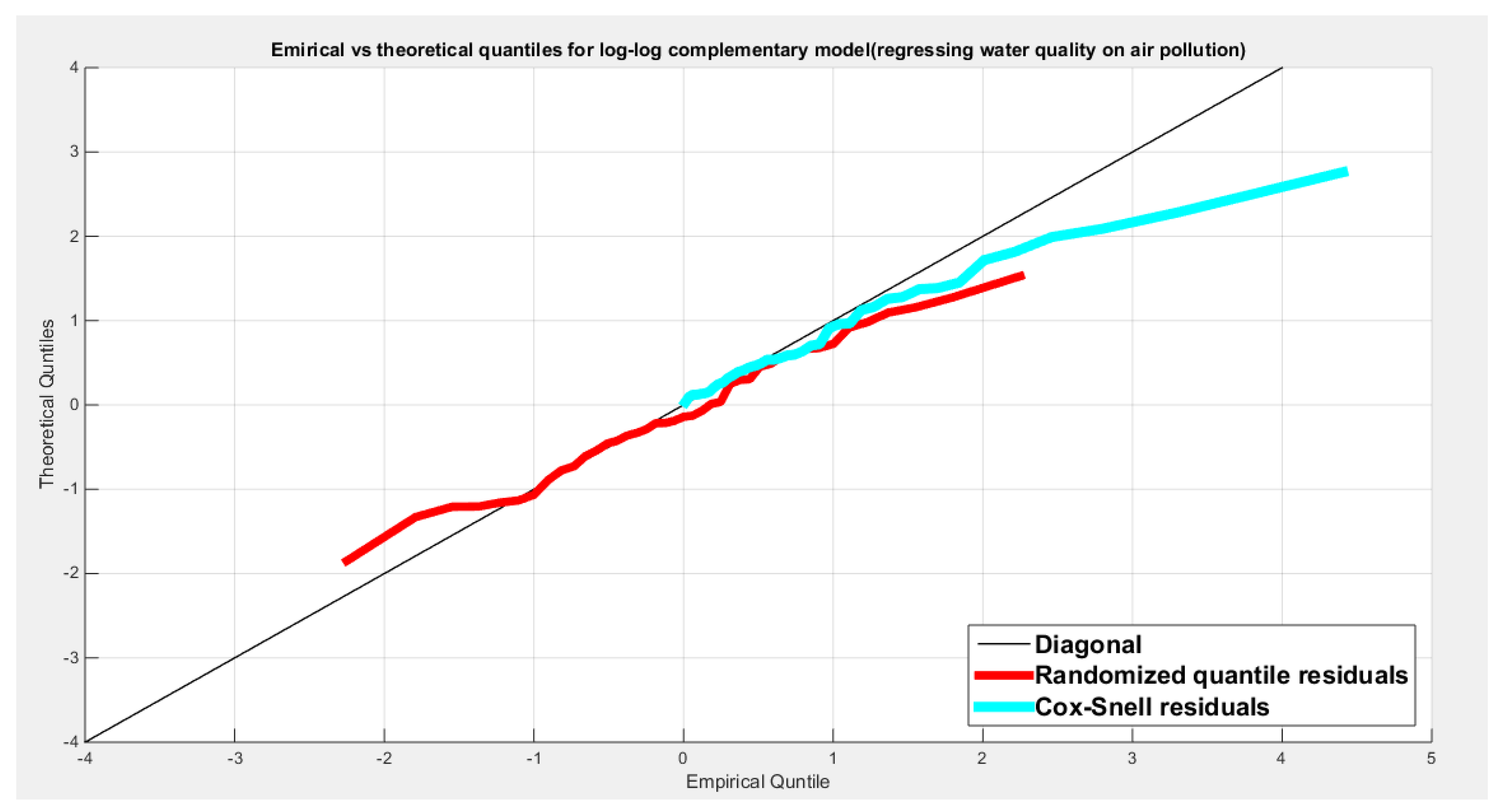
Figures for the Log-log complementary Model

Figure 6. Shows the decreasing estimated curve for the median against the transformed predictor.

Figure 6. Shows the decreasing estimated curve for the median against the transformed predictor.

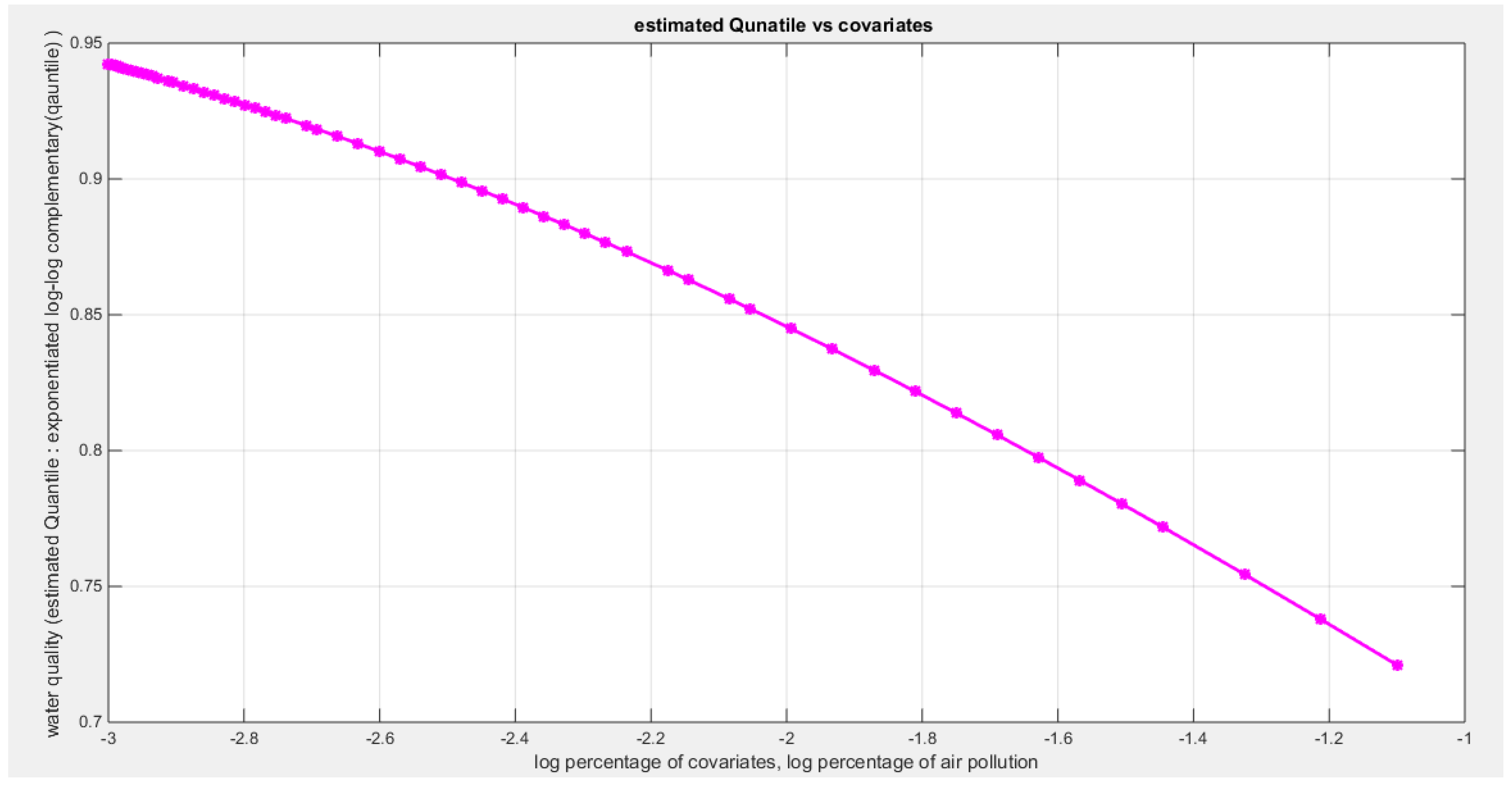
Figure 7. Shows the predictors vs. the residuals of both types. Both curves show no specific trend and they are randomly related.

Figure 7. Shows the predictors vs. the residuals of both types. Both curves show no specific trend and they are randomly related.

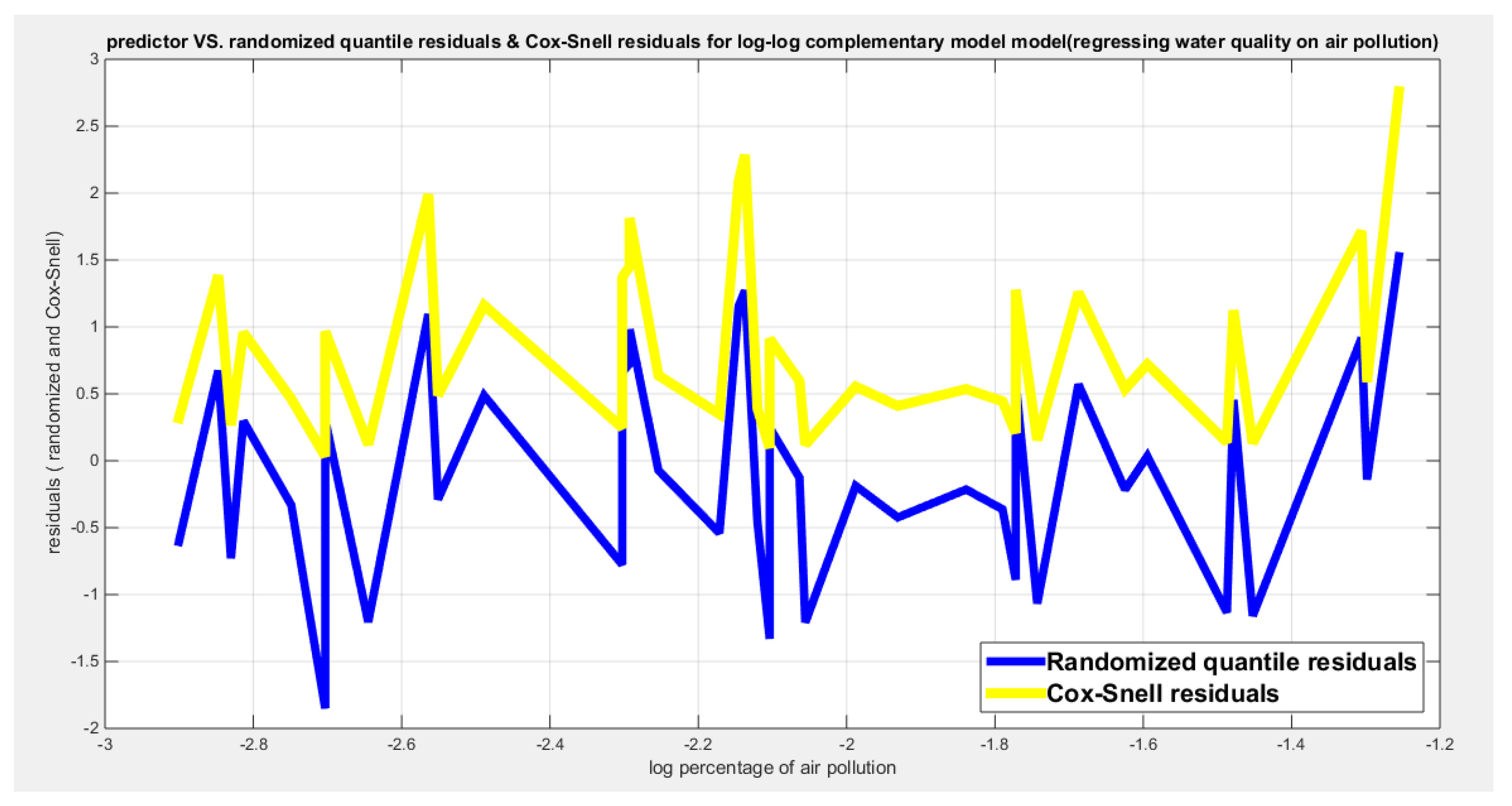
Figure 8. Shows the residuals against the predictors. No specific trend is there and they are randomly scattered. This behavior is clear and obvious for both types of residuals.

Figure 8. Shows the residuals against the predictors. No specific trend is there and they are randomly scattered. This behavior is clear and obvious for both types of residuals.

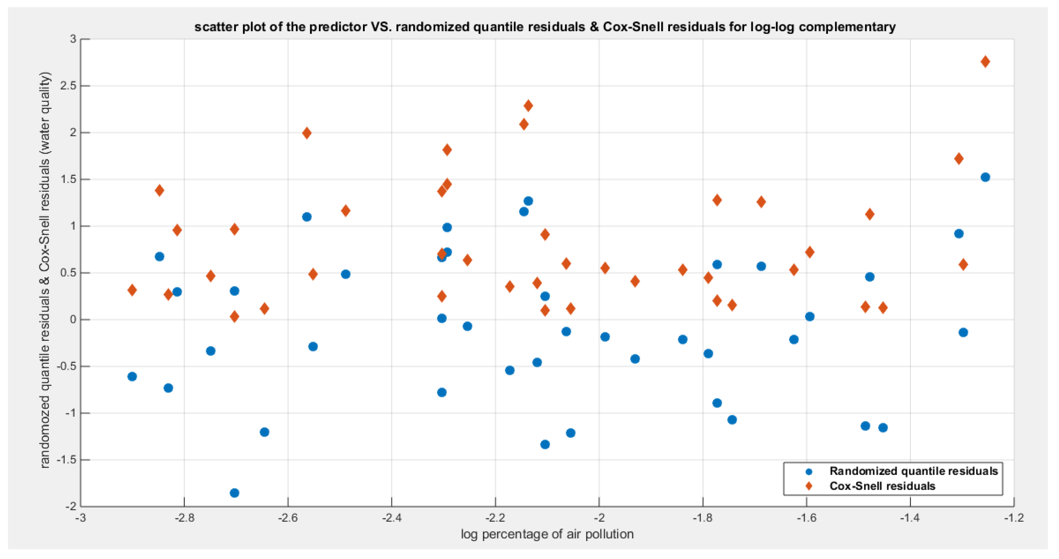
Figure 9. Shows the QQ plot of the empirical quantiles for both residuals . The randomized quantile residuals are more or less perfectly aligned to the diagonal than the Cox Snell residual. Cox-Snell residuals are nearly aligned to diagonal at the lower end than at the center and upper tail.

Figure 9. Shows the QQ plot of the empirical quantiles for both residuals . The randomized quantile residuals are more or less perfectly aligned to the diagonal than the Cox Snell residual. Cox-Snell residuals are nearly aligned to diagonal at the lower end than at the center and upper tail.

Figures for the Log-log median Model

Figure 10. Shows the decreasing estimated curve for the median against the transformed predictor.

Figure 10. Shows the decreasing estimated curve for the median against the transformed predictor.

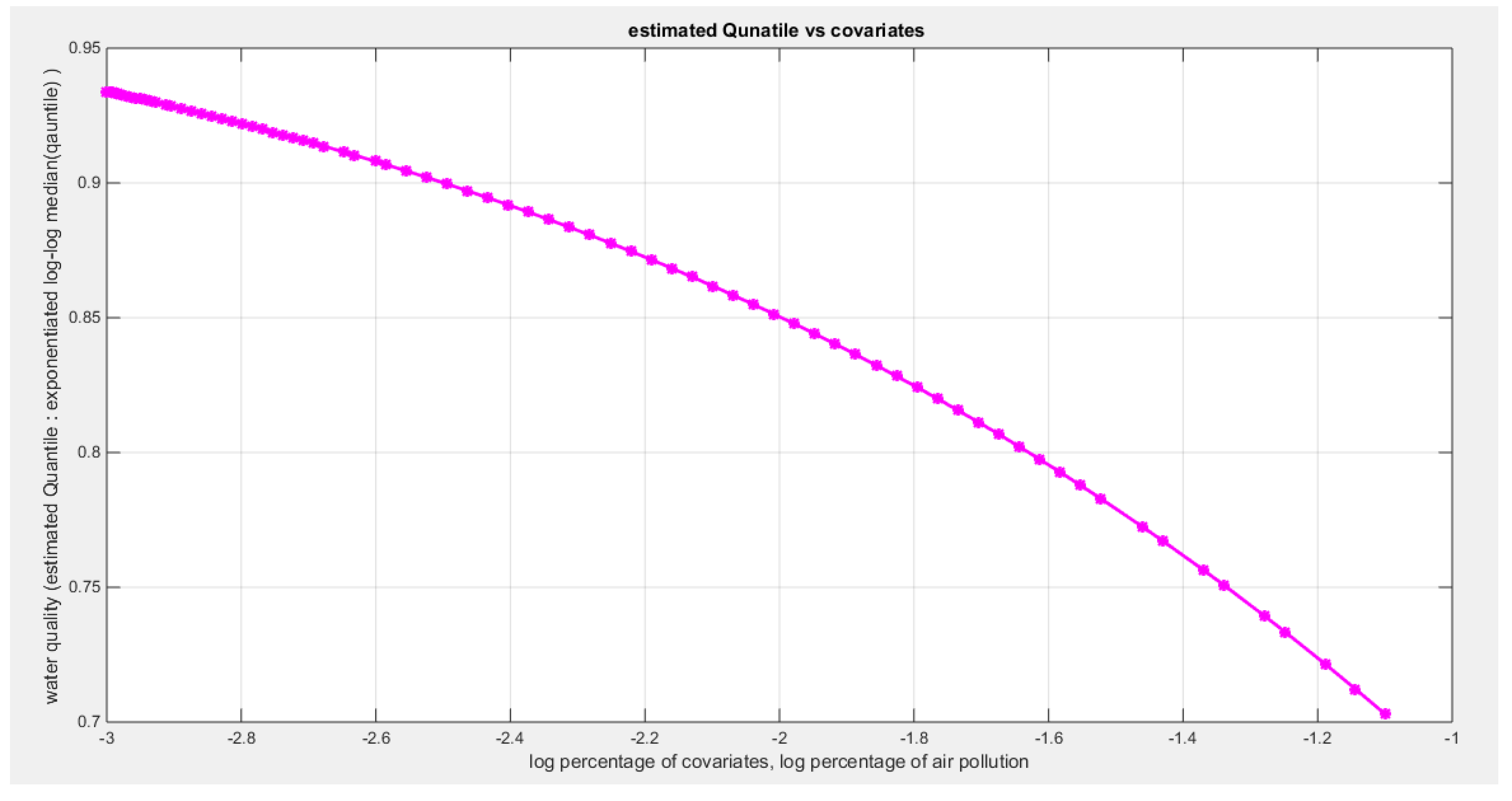
Figure 11. Shows the predictors vs. the residuals of both types. Both curves show no specific trend and they are randomly related.

Figure 11. Shows the predictors vs. the residuals of both types. Both curves show no specific trend and they are randomly related.

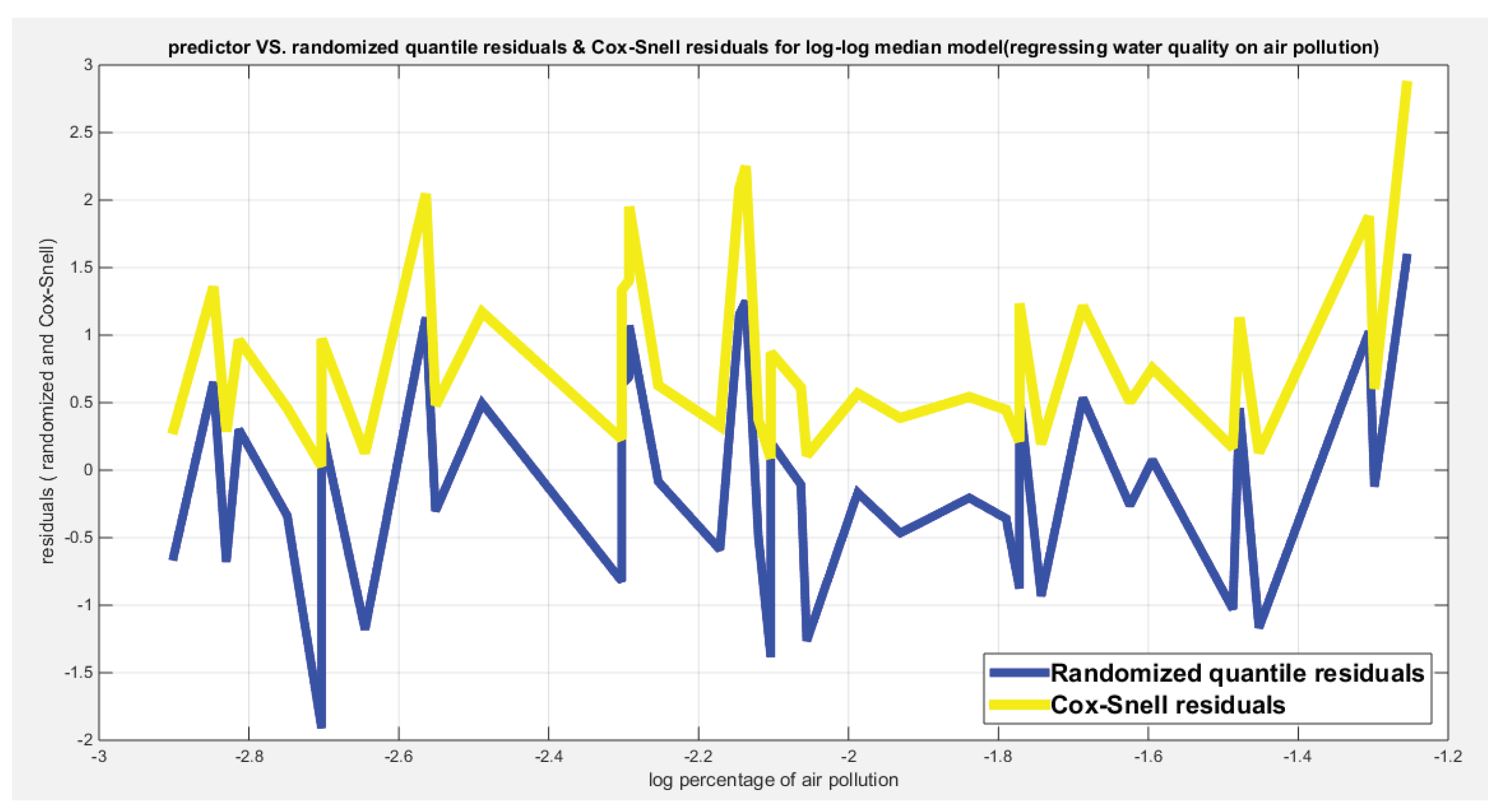
Figure 12. Shows the residuals against the predictors. No specific trend is there and they are randomly scattered. This behavior is clear and obvious for both types of residuals.

Figure 12. Shows the residuals against the predictors. No specific trend is there and they are randomly scattered. This behavior is clear and obvious for both types of residuals.

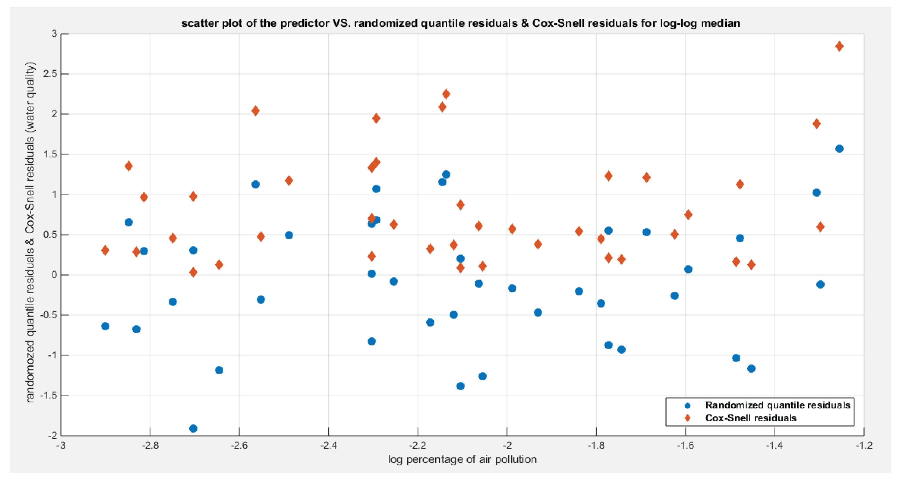
Figure 13. Shows the QQ plot of the empirical quantiles for both residuals. The randomized quantile residuals are more or less perfectly aligned to the diagonal than the Cox Snell residual. Cox-Snell residuals are nearly aligned to diagonal at the lower end than at the center and upper tail.

Figure 13. Shows the QQ plot of the empirical quantiles for both residuals. The randomized quantile residuals are more or less perfectly aligned to the diagonal than the Cox Snell residual. Cox-Snell residuals are nearly aligned to diagonal at the lower end than at the center and upper tail.

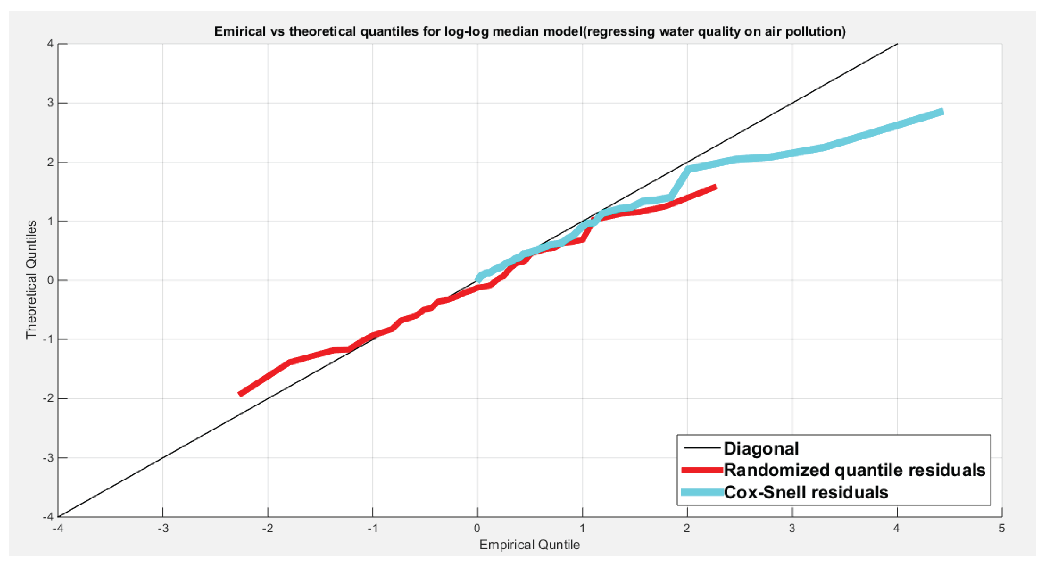
From the above table and figures, the three models show minimal difference in the statistical indices, they all fit the data and even if the link functions are monotonically increasing or decreasing, the estimated curve is a decreasing function in the predictor. That is to mean, the increased percentage of air pollution decreases the quality of water and this account for about 24 %. Other predictors should be investigated and added to the OECD platform. The coefficient has different sign in the log-log model; it has a positive sign while it has a negative sign in the other model. The QQ plot of the empirical quantiles against the theoretical quantiles shows almost near perfect alignment of the randomized quantile residuals with the diagonal all through its course in comparison of the alignment of the Cox-Snell residuals with the diagonal, which shows near alignment with the diagonal at the lower tail only, as it is not perfectly aligned at the center and the upper tail like the QR. the Kendall tau denotes that the relation between the residuals and the predictors are not statistically significant as the tau is 0.0159 and the associated p value is 0.8927.The plot depicting this relation shows no specific trend and the residuals are randomly scattered all over the different values of the transformed predictors. The figures for the 3 models have similar patterns.

References

- Attia, I. (2024). A Novel Unit Distribution Named as Median Based Unit Rayleigh (MBUR): Properties and Estimations. [CrossRef]
- Garcia-Papani, F.; Leiva, V.; Uribe-Opazo, M.A.; Aykroyd, R.G. Birnbaum-Saunders spatial regression models: Diagnostics and application to chemical data. Chemometrics and Intelligent Laboratory Systems 2018, 177, 114–128. [Google Scholar] [CrossRef]
- Korkmaz, M.Ç.; Chesneau, C. On the unit Burr-XII distribution with the quantile regression modeling and applications. Computational and Applied Mathematics 2021, 40, 29. [Google Scholar] [CrossRef]
- Korkmaz, M.Ç.; Chesneau, C.; Korkmaz, Z.S. On the Arcsecant Hyperbolic Normal Distribution. Properties, Quantile Regression Modeling and Applications. Symmetry 2021, 13, 117. [Google Scholar] [CrossRef]
- Korkmaz, M.Ç.; Chesneau, C.; Korkmaz, Z.S. A new alternative quantile regression model for the bounded response with educational measurements applications of OECD countries. Journal of Applied Statistics 2023, 50, 131–154. [Google Scholar] [CrossRef] [PubMed]
- Kumar, D.; Dey, S.; Ormoz, E.; MirMostafaee, S.M.T.K. Inference for the unit-Gompertz model based on record values and inter-record times with an application. Rendiconti Del Circolo Matematico Di Palermo Series 2 2020, 69, 1295–1319. [Google Scholar] [CrossRef]
- Leão, J.; Leiva, V.; Saulo, H.; Tomazella, V. Incorporation of frailties into a cure rate regression model and its diagnostics and application to melanoma data. Statistics in Medicine 2018, 37, 4421–4440. [Google Scholar] [CrossRef] [PubMed]
- Leiva, V. (Ed.). (2016). The Birnbaum-Saunders distribution. Elsevier.
- Leiva, V.; Santos, R.A.D.; Saulo, H.; Marchant, C.; Lio, Y. Bootstrap control charts for quantiles based on log-symmetric distributions with applications to the monitoring of reliability data. Quality and Reliability Engineering International 2023, 39, 1–24. [Google Scholar] [CrossRef]
- Marchant, C.; Leiva, V.; Cysneiros, F.J.A. A Multivariate Log-Linear Model for Birnbaum-Saunders Distributions. IEEE Transactions on Reliability 2016, 65, 816–827. [Google Scholar] [CrossRef]
- Mazucheli, J.; Alves, B.; Korkmaz, M.Ç. The Unit-Gompertz Quantile Regression Model for the Bounded Responses. Mathematica Slovaca 2023, 73, 1039–1054. [Google Scholar] [CrossRef]
- Mazucheli, J.; Alves, B.; Korkmaz, M.Ç.; Leiva, V. Vasicek Quantile and Mean Regression Models for Bounded Data: New Formulation, Mathematical Derivations, and Numerical Applications. Mathematics 2022, 10, 1389. [Google Scholar] [CrossRef]
- Mazucheli, J.; Leiva, V.; Alves, B.; Menezes, A.F.B. A New Quantile Regression for Modeling Bounded Data under a Unit Birnbaum–Saunders Distribution with Applications in Medicine and Politics. Symmetry 2021, 13, 682. [Google Scholar] [CrossRef]
- Mazucheli, J.; Menezes, A.F.B.; Chakraborty, S. On the one parameter unit-Lindley distribution and its associated regression model for proportion data. Journal of Applied Statistics 2019, 46, 700–714. [Google Scholar] [CrossRef]
- Mazucheli, J.; Menezes, A.F.B.; Fernandes, L.B.; De Oliveira, R.P.; Ghitany, M.E. The unit-Weibull distribution as an alternative to the Kumaraswamy distribution for the modeling of quantiles conditional on covariates. Journal of Applied Statistics 2020, 47, 954–974. [Google Scholar] [CrossRef] [PubMed]
- Noufaily, A.; Jones, M.C. Parametric Quantile Regression Based on the Generalized Gamma Distribution. Journal of the Royal Statistical Society Series C: Applied Statistics 2013, 62, 723–740. [Google Scholar] [CrossRef]
- Sánchez, L.; Leiva, V.; Galea, M.; Saulo, H. Birnbaum-Saunders Quantile Regression Models with Application to Spatial Data. Mathematics 2020, 8, 1000. [Google Scholar] [CrossRef]
- Sánchez, L.; Leiva, V.; Galea, M.; Saulo, H. Birnbaum-Saunders quantile regression and its diagnostics with application to economic data. Applied Stochastic Models in Business and Industry 2021, 37, 53–73. [Google Scholar] [CrossRef]
- Sánchez, L.; Leiva, V.; Saulo, H.; Marchant, C.; Sarabia, J.M. A New Quantile Regression Model and Its Diagnostic Analytics for a Weibull Distributed Response with Applications. Mathematics 2021, 9, 2768. [Google Scholar] [CrossRef]
- R packages:, R. Koenker, quantreg: quantile regression, 2021, https://CRAN.R- project.org/package=quantreg. R package version 5.86.
- J. Mazucheli, B. J. Mazucheli, B. Alves, Ugomquantreg: quantile regression modeling for unit-Gompertz responses, 2021a, R package version 1.0.0.
- J. Mazucheli, A.F.B. J. Mazucheli, A.F.B. Menezes, unitBSQuantReg: unit-Birnbaum-Saunders quantile regression, 2020, https://github.com/AndrMenezes/unitBSQuantReg. R package version 0.1.0.
- A.F.B. Menezes, Uwquantreg: unit-Weibull quantile regression, 2020, https://github.com/AndrMenezes/uwquantreg. R package version 0.1.0.
- R Core Team, R: A Language and Environment for Statistical Computing, R Foundation for Statistical Computing, Vienna, Austria, 2020. Available online: https://www.R-project.org/.