
Submitted:
28 January 2025
Posted:
29 January 2025
You are already at the latest version
Abstract
As the maximum likelihood method is the most commonly used method for parameters estimation being unbiased, consistent, efficient, and asymptotically normal, MLE is used to fit the new distribution (MBUW). But in small to moderate sample size, this MLE estimator is biased unlike the MLE estimators obtained from large sample sizes. In this paper, the Bias-corrected approach for this distribution is discussed and applied to real data analysis. The MLE estimators of MBUW obtained from some optimization techniques like derivative free Nelder Mead algorithm suffers from significant high correlation that is reflected on high covariance between the parameters. Also this association between the parameters affects the variances which may be inflated enough to approach infinity hampering construction of confidence intervals for each parameter. This problem may arise with any optimization technique which necessitates remedies trying to fix it. The author also elaborates a variance correction approach heavily relaying on re-parameterizing the negative log likelihood.
Keywords:
Cox and Snell bias-correction
; median based unit weibull
; maximum likelihood estimators
; Monte Carlo simulation
; variance-corrected MLE
; bias-corrected MLE
Introduction
The most commonly used parameter estimation method is the maximum likelihood estimation (MLE), which is crucial for any probability distribution (Pawitan, 2001),(Millar, 2011). MLE estimator has many advantageous properties such as asymptotically unbiased, consistent, efficient and asymptotically normally distributed. These properties depend mainly on large sample size. In small to moderate sample size some of these properties like un-biasness may be violated. The error obtained from the difference between the expected value of the parameter and the true value of the parameter is reduced as the sample size increases. For that reason, the researchers develop almost unbiased estimators for different distributions. To mention some of them: (Saha & Paul, 2005),(Cordeiro et al., 1997), (Giles, 2012) (Cribari-Neto & Vasconcellos, 2002), (Lemonte et al., 2007), (Giles, & Feng, 2009),(Giles, 2012), (Schwartz et al., 2013), (Giles et al., 2013), (Teimouri & Nadarajah, 2013), (Zhang & Liu, 2017), (Singh et al., 2015), (Lagos-Àlvarez, et al., 2011), (Schwartz & Giles, 2016), (Wang & Wang, 2017), (Ling & Giles, 2014), (Lemonte, 2011), (Mazucheli & Dey, 2018), (Reath, 2016), and (Teimouri & Nadarajah, 2016), and references cited therein.
It is possible to approximate the bias of the MLE of the estimated parameter for a single parameter distribution to the even if the estimated parameter is not in a closed form expression (Bartlett, 1953a) (Haldane & Smith, 1956), (Bartlett, 1953b) and (Haldane, 1953)derived the analytic approximations for two-parameters log-likelihood functions utilizing the Tayler series expansions that may be tough for multi-parameter distributions as illustrated by (Shenton & Bowman, 1963).
Many approaches have been proposed to correct the bias for MLE. The first approach is called the “corrective approach”. It is the analytical methodology advocated by (Cox & Snell, 1968). It is an analytical expression for the bias to of the MLE estimators, then using these expressions to bias-correct the MLE estimator yielding estimators that are unbiased to . The second approach is parametric Bootstrap resampling technique advised by (Efron, 1982). It is also a second-order bias correction. The bias-correction is carried out numerically without developing analytical expression for the bias function. The third approach is called “preventive approach” recommended by (Firth, 1993). It is analytic procedure that mandates modification of the score function of the log-likelihood function before solving for the MLEs and it reduces the bias to the order . The first two approaches have unsophisticated mathematical expressions which renders them appealing and simple to calculate.
The BMUW distribution has been discussed in earlier work by the author (Iman M. Attia, 2024) as regards properties and some methods of estimation with applications on real data analysis. The new distribution has the following PDF, CDF and quantile function respectively, as shown in equations (1-3)
This distribution is defined on the unit interval. It can accommodate skew data expressed as proportions. The distribution can have a bathtub or unimodal shapes according to the parameters.
In this paper, the author discusses the bias-corrected MLE approach and the variance-corrected MLE technique. The paper is constructed into sections. Methods are contained in section1 and section 2. In section 1, the author explains the corrective procedure for the bias of the MLE estimators. In section 2, the author derives the analytic function for the bias of MLE estimators for the MBUW distribution. Results are revealed in section 3. In section 3, the author describes the variance-corrected MLE procedure for MBUR and implements this approach on real data. Discussion is carried out in section 4. In section 4, the author deploys the bias-corrected MLE on real data comparing values of the estimated parameters obtained from the variance-corrected MLE with the values obtained by bias-corrected approach. In section 5, conclusions and recommendations are elucidated.
Methods
1. Section 1
Bias-Corrected MLE
Let be a p-dimensional unknown parameter vector and be the log-likelihood function for a sample of n
observations. Assume this log-likelihood is regular with respect to all
derivatives up to and including those of third order. The joint cumulants of
the log-likelihood derivatives are defined as follows in equations (4-6)
The derivative of these cumulants are defined as in equation (7)
The expressions in eqautions (4-7) are assumed to be .
(Cox & Snell, 1968) revealed that when the sample data are independent (but not necessarily identically distributed) the bias of the sth element of the MLE of , is calculated as
where : and is the element of the inverse of the expected information matrix .
(Cordeiro & Klein, 1994) consequently established that equation (8) yet maintains if the data are non-independent and that it can be disclosed as
The bias equation in (9) is largely simpler to calculate than in (8), because it does not include terms of the form given in (6).
Defining the following terms in equations (10-11):
and collecting terms up into matrices
The bias of the MLE of in (9) can be rephrased in the convenient form equation (12):
where and , the value of is obtained by solving the roots of log-likelihood equations using the numerical methods. means vectorization operator, which stacks the columns of the matrix in question one above the other, forming one extended column vector. Hence the bias adjusted-MLE is defined in equation (13) as
One of the benefits of this method is that these expressions can be calculated when solving for the root of the log-likelihood equations do not disclose an analytic closed-form solution. In such circumstances, the bias-corrected MLE can be easily obtained by means of standard numerical methods, and is unbiased
2. Section 2
Bias Reduction and the MBUW
The PDF of MBUW satisfies the regularity conditions. The first order partial derivatives of log-likelihood with respect to alpha and beta parameters are defined in equation (14-15) as follows:
Equations (16-24) are the higher order derivatives (for one observation):
Taking expectation of the above derivative is carried out using Monte Carlo integration; see equations (25-31). The following integral can be calculated using Monte Carlo integration and it is a fixed number. The author underwent trapezoid method for integration. Substituting the estimated parameters alpha and beta for each data set, the following integrals can be calculated and are fixed value for each dataset.
Define the following quantities:
The information matrix is where n is the number of observations.
Defining ; and
Upon using Cordeiro and Klein (1994) modification of the Cox and Snell (1968) result; the The bias-adjusted estimators can be obtained as in equation (32)
Where and
Results
3. Section 3
3.1. Variance-Corrected MLE Procedure and MBUW
Maximum likelihood estimators for the parameters of MBUW distribution may have large variances or infinite variances. Because the parameters are correlated they also have large covariance. The surface of the log-likelihood function may exhibits a flat shape which is reflected by multiple pair of estimators that fit the distribution. Also the estimators may be unstable. Inspecting the surface of the negative log-likelihood function can depicts the pairs of parameters which attain the minimal negative likelihood (nLL) values. The approach used by the author in this paper is to obtain these pairs and find the relationship between them and define one parameter in term of the other. Then reparameterize the negative likelihood function and scale one of the parameter in log scale. Then estimate this parameter and back substitute in the relationship to obtain the other parameter. The variance of the parameter obtained from the MLE is obtained by inversing the fisher information while the parameter defined in the relationship is obtained using the delta method.
3.2. Real Data Analysis Using Variance-Corrected MLE
These data were mentioned by the author in previous work (Iman M. Attia, 2024)
Steps of the technique used by the author:
- 1-
- Inspect the surface of the nLL.
- 2-
- Extract the pairs of alpha and beta parameter that minimize the nLL. The range of the alpha and beta were divided into equally spaced 500 points. The range differs according to the datasets. These ranges were chosen according to the results obtained from MLE using Nelder Mead algorithm results.
- 3-
- Define beta in terms of alpha by fitting the best curve for this relationship.
- 4-
- Reparameterize the nLL using this relationship.
- 5-
- Estimate alpha parameter.
- 6-
- Back substitute in the relationship to obtain the beta parameter.
- 7-
- Use inverse fisher obtained from the MLE to obtain variance of the alpha and use the delta method to obtain the variance of the beta.
- 8-
- Use goodness of fit test like the KS-test, AD-test and CVM-test evaluate the fitting of the distribution to data.
3.2.1. First Dataset: Dwelling Without Basic Facilities
- 1-
- Inspecting the surface of nLL. Figure 1 illustrates this surface of which has a flat part.
- 2-
- Extracting the pairs of the parameters that minimize the nLL. These pairs were 130 pairs. Figure 2 illustrates the relation between these parameters.
- 3-
-
Define the relationship between alpha and beta by fitting the best curve depicting this relationship. see equations (1-3)For exponentional decay model:For polynomial model :For reciprocal model:
- 4-
- Reparameterize the nLL by substituting each beta in LL. see equation(4)
- 5-
- Use the Nelder Mead algorithm to obtain MLE estimator for the alpha and use the inverse fisher to obtain the variance of the alpha.
- 6-
- Back substitute in each model to obtain the beta.
- 6-
-
Use the delta method to obtain the variance of the beta as follows: delta method is defined as see equations(5-8)For the three models it is defined as:For the exponen. Decay :For the quadratic polynomial:For the reciprocal model
- 8-
- Use goodness of fit techniques such as KS-test to test the null hypothesis testing the fitness of the data to the theoretical distribution with the estimated parameters.
The results of the above procedure is shown in Table 1
The exponential decay has the following metrics: residual sum of square (SRR) value 0.0493, R sqaure value 0.9961, and root mean square error (RMSE) value 0.0195. The reciprocal model has the following values for RSS, R squared and, RMSE: 0.1198, 0.9905 and, 0.0305 respectively. The quadratic model has the following values for RSS, R squared and, RMSE: 0.2442, 0.9807 and 0.0435 respectively.
The analysis revealed the marked reduction in the variance for both alpha and beta. This has tremendous effect when constructing the confidence interval (CI) as it becomes narrower. The values of the parameters were not unique; they show small changes when changing the initial guess. The values with minimum variance were chosen to be reported as long as they failed to reject the null hypothesis. The other metrics like nLL, AIC, corr AIC, BIC, and HQIC are the same as the one that are obtained from conducting Nelder mead algorithm to estimate MLE for both parameters. And this is reflected on the graph of the theoretical CDF, graph of PDF and the QQ plot. They are all the same as if there is the same pattern if the parameters give the same nLL. The values of alpha and beta are nearly equal and the variances show minor differences among the models but the quadratic model has the minimal variance.
3.2.2. Second Dataset: Quality of the Support Network
- 1-
- Inspecting the surface of nLL. Figure 3 illustrates this surface of which has a flat part.
- 2-
- Extracting the pairs of the parameters that minimize the nLL. These pairs were 16 pairs. Figure 4 illustrates the relation between these parameters.
- 3-
- Define the relationship between alpha and beta by fitting the best curve depicting this relationship. See equation (9)
For linear model:
The linear model has the following values for RSS, R squared and, RMSE: 0.0029, 0.9977 and, 0.014 respectively.
The variance of both parameters show marked reduction. The confidence (CI) interval becomes narrower. The distribution fits the data. Other metrics are more or less the same as the results obtained from MLE using the Nelder Mead algorithm. The parameters do not change with the initial guess.
3.2.3. Third Dataset: Voter Turnout Dataset
- 1-
- Inspecting the surface of nLL. Figure 5 illustrates this surface of which has a flat part.
- 2-
- Extracting the pairs of the parameters that minimize the nLL. These pairs were 51 pairs. Figure 6 illustrates the relation between these parameters.
- 3-
- Define the relationship between alpha and beta by fitting the best curve depicting this relationship. See equation(10-11)
For quadratic model:
For the power law model:
Follow the steps from 4 to 8, for the delta method see equation (12-13):
For the power law:
For the quadratic polynomial:
The power law model has the following values for RSS, R squared and RMSE: 0.0289, 0.997, and 0.024 respectively. The quadratic model has the following values for RSS, R squared and RMSE: 0.0422, 0.9956, and 0.0291 respectively.
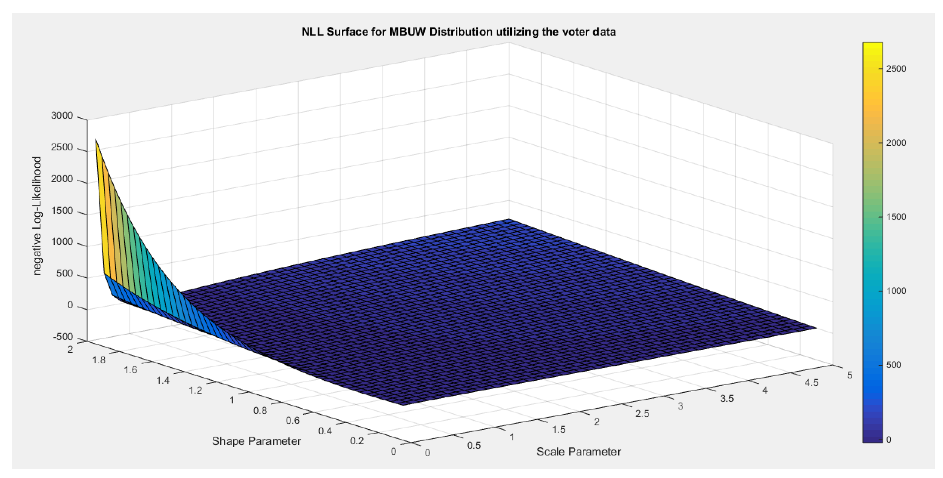
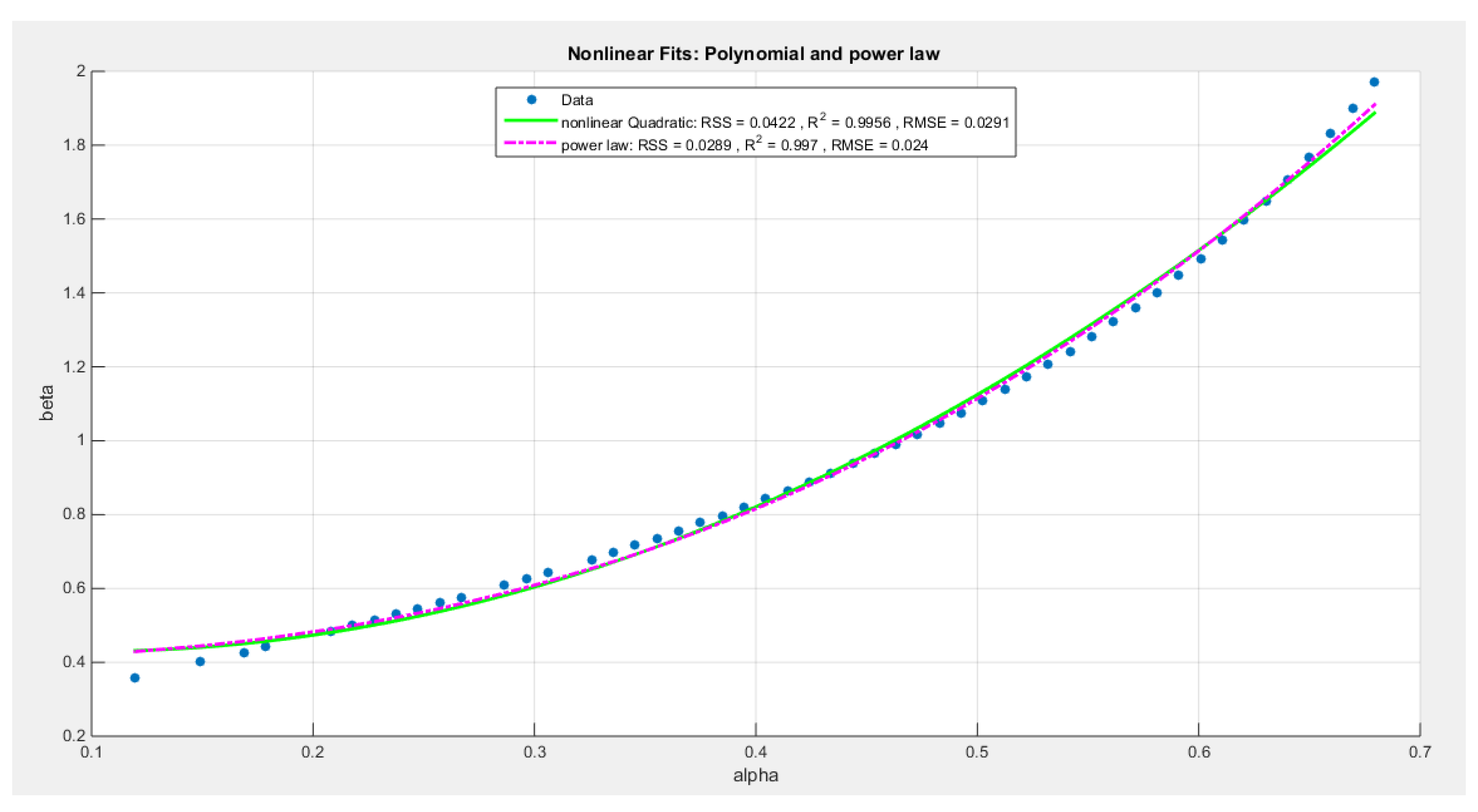
Figure 5.
negative likelihood surface using the Voter dataset.
Figure 6.
Nonlinear models for the voter dataset (increasing convex relationship between alpha and the beta), with residual sum of squares (RSS), R^2 and root of mean square error(RMSE) illustrated in the figure for each curve, high lightening that the power law is the best model followed by the polynomial( quadratic).
Table 4 illustrates the results of using these models to re-parameterize the nLL and running MLE using the Nelder Mead algorithm by Matlab.
From Table 4, the analysis revealed that the metrics between the two models are minor but it is in favor of the polynomial model over the power law model. This is due to the fact that it has more negative values of the nLL, AIC, corr AIC, BIC, HQIC than the power law has. It also has less value for the KS-test, AD and CVM than the power law has. All these metrics favor the quadratic model over the power law model, although the power law model better describes the relationship between beta and alpha than the quadratic model as indicated by the metrics; SRR, R squared and RMSE.
3.2.4. Fourth Dataset: Flood Data
- 1-
- Inspecting the surface of nLL. Figure 7 illustrates this surface of which has a flat part.
- 2-
- Extracting the pairs of the parameters that minimize the nLL. These pairs were 139 pairs. Figure 8 illustrates the relation between these parameters.
- 3-
- Define the relationship between alpha and beta by fitting the best curve depicting this relationship. See equations(14-16)
For exponentional decay model:
For polynomial model:
For reciprocal model:
Follow the steps from 4 to 8
The exponential decay model has the following values for RSS, R squared and, RMSE: 0.2612, 0.969, and 0.0435 respectively. The quadratic model has the following values for RSS, R squared and, RMSE: 2.1792, 0.7412 and 0.1257 respectively. The reciprocal model has the following values for RSS, R squared and, RMSE: 2.9594, 0.6485 and, 0.1464 respectively.
Table 5 illustrates the results obtained from re-parameterizing the nLL function using these 3 different models.
In the analysis, initial guess may cause the estimators to change their values, but the variance and the goodness of fit may judge or add to the control if this initial guess, causing the new value, should be taking into consideration or discarded. In this situation the low variance estimator associated with goodness of fit test supporting the fitting distribution are the corner stones to choose the estimators values and hence consider the stability of the estimators.
The variance of alpha obtained by exponential decay model is the lowest than other variances obtained by quadratic and reciprocal model. The opposite is true concerning the variance of the beta. The variances of both alpha and beta for the reciprocal model are nearly equal as well as the standard errors. This is reflected by a narrower CI for both alpha and beta estimators obtained from the reciprocal model. This is not true concerning the interval for the beta estimator obtained from exponential decay model which is the widest among the other CI intervals obtained from other models. So the reciprocal model may outperform the exponential model
3.2.5. Fifth Dataset: Time Between Failures Data Set
- Inspecting the surface of nLL. Figure 9 illustrates this surface of which has a flat part.
- Extracting the pairs of the parameters that minimize the nLL. These pairs were 246 pairs. Figure 10 illustrates the relation between these parameters.
- Define the relationship between alpha and beta by fitting the best curve depicting this relationship. See equations (17-19)
For exponential decay model:
For polynomial model:
For reciprocal model:
Follow the steps from 4 to 8
The exponential decay model has the following values for RSS, R squared and, RMSE: 0.1239, 0.9957, and 0.0225 respectively. The reciprocal model has the following values for RSS, R squared and, RMSE: 0.5583, 0.9808 and, 0.0477 respectively. The quadratic model has the following values for RSS, R squared and, RMSE: 0.9653, 0.9668 and 0.0628 respectively.
Table 6 illustrates the results obtained from re-parameterizing the nLL function using these 3 different models.
The analysis of the above models are comparable the variances are approximately equal, the estimator are also nearly equal. Any model can be chosen. The CI is narrow. The estimators are stable regardless the initial guess used as the estimator, variance and the goodness of fit results does not change. This is peculiar for this dataset.
3.2.6. Sixth Dataset: Capacity Factor Data Set
- Inspecting the surface of nLL. Figure 11 illustrates this surface of which has a flat part.
- Extracting the pairs of the parameters that minimize the nLL. These pairs were 80 pairs. Figure 22 illustrates the relation between these parameters.
- Define the relationship between alpha and beta by fitting the best curve depicting this relationship. See equation (20-22)
For exponential decay model:
For polynomial model:
For reciprocal model:
Follow the steps from 4 to 8
The exponential decay model has the following values for RSS, R squared and, RMSE: 0.0442, 0.9954, and 0.0237 respectively. The reciprocal model has the following values for RSS, R squared and, RMSE: 0.2843, 0.9701 and, 0.06 respectively. The quadratic model has the following values for RSS, R squared and, RMSE: 0.3523, 0.963 and 0.0668 respectively.
Table 7 illustrates the results obtained from re-parameterizing the nLL function using these 3 different models.
The results of the three models are comparable. The variances of parameters are small and are approximately equal between the 3 models. The CI is small. Any model can be chosen.
Discussion
Section 4
Real Data Analysis Using Bias-Corrected MLE Approach
The bias-corrected approach is applied on the same datasets to be compared with the previously estimated parameters obtained from the variance-corrected MLE approach discussed in section 3. These datasets are the first, fifth, and sixth sets.
Table 8 shows the values of parameters before and after the correction along with the bias values. Table 9 shows the metrics after correction by equation 32.
Figure 13, Figure 14 and Figure 15 show the CDF and QQ plot for the above data before and after correction for the mentioned values of the parameters.
Table 8 shows minor reduction for the metrics for all the datasets after correction. The variance covariance matrix for each data set exhibit minor variance for each parameter and minimal negative covariance between them reflecting the inverse relationship between them as was illustrated from inspecting the nLL surface in section 3. Figure 13, Figure 14 and Figure 15 show minor drift between the CDF graph before and after the correction for the dwelling data set and almost no change between the two graphs for the time between failures dataset and factors affecting unit capacity datasets. The inverse of information matrix which represents the variance covariance matrix is positive definite, while the other datasets (quality of support network, voter, and flood datasets have non-definite positive variance covariance matrix, although the KS test results shows fitting of the distribution to these datasets, so the author did not show the results).
The variance-corrected approach leads to marked reduction of the variances and correlation between parameters. The author used the finite difference approach for all datasets and it resulted into zero correlation between the parameters especially for the data sets with negative correlation and when using the reciprocal models (but the results are unpublished now). Using the delta method induces more reduction than the reduction obtained by the central finite difference method. The resulting uncorrelated estimators with these reduced variances yielded distributions that can fit the different datasets. On the other hand, the bias-corrected approach gives positive definite variance-covariance matrix only in three data sets in contrast to the variance-corrected approach by which all matrices were positive definite. Also the bias-corrected approach heavily depends on the expectations of the higher order derivatives and depends on how to solve for this integration. The method used in solving this integration dramatically impact the information matrix and hence the variance-covariance matrix. The variance-corrected approach yields robust results than methods like generalized method of moments and percentile methods used previously by the author. These latter methods have resulted in large variances and correlated parameters, although their variances are smaller in comparison to the MLE used by Nelder Mead optimizer but still they are inflated. The procedure used in this paper dramatically reduced the variance. If the distribution fits the data set with specific parameter values, there is a fixed pattern in the QQ plot. The datasets exhibit skewness and kurtosis. The visualization of the nLL surface for each dataset helps a lot to anticipate the results of the estimation process, the uniqueness and identifiability of the estimators, the correlation between the parameters. The chosen value of parameters depend on many factors the most is the chosen estimators should have also the least variance, goodness of fit test shows fitness of the distribution, the metrics like nLL, AIC, CAIC, BIC and HQIC should have the highest negative values. The estimators are preferable to be stable and not show marked changes to the initial guess especially when using iterative techniques which is the actual case.
Section 5
Conclusion
The variance-corrected approach and the bias-corrected approach are valuable techniques used after initial estimation of the MBUW parameters by approaches like MLE using whatever optimizer according to the data characteristics or using generalized methods of moments or percentile methods as these two procedures do not control for correlation between the parameters. So in real world practice, one can start with MLE using Nelder Mead optimization or any other optimizer and if the data characteristics have large impact on the variance, one can shift to methods like generalized method of moments or percentile methods which further reduce the variance but still their variances are large. Visualizing the surface of nLL helps a lot to anticipate the parameter values that can cause the distribution fit the data and also helps in initial guess of the parameters. With the aid of this inspection, variance-corrected and bias-corrected approach ameliorate the inflated variance and help reducing the correlation between the parameters to yield more robust results.
Future Works
For the three datasets exhibiting non positive definite variance-covariance matrix and similar situations, use the Bayesian inference may help in estimation process.
Ethics approval and consent to participate
Not applicable.
Consent for publication
Not applicable
Availability of data and material
Not applicable. Data sharing does not apply to this article as no datasets were generated or analyzed during the current study.
Competing interests
The author declares no competing interests of any type.
Authors’ contribution
AI carried the conceptualization by formulating the goals, and aims of the research article, formal analysis by applying the statistical, mathematical, and computational techniques to synthesize and analyze the hypothetical data, carried the methodology by creating the model, software programming and implementation, supervision, writing, drafting, editing, preparation, and creation of the presenting work.
Funding
No funding resources. No funding roles in the design of the study and collection, analysis, and interpretation of data and in writing the manuscript are declared.
Acknowledgment
Not applicable.
Appendix A
The following are the values of alpha and beta obtained from visualizing or inspecting the nLL surface of the quality of support network dataset:
alpha=[0.119639279, 0.129458918, 0.158917836, 0.168737475, 0.178557114, 0.188376754, 0.198196393, 0.227655311, 0.23747495, 0.257114228, 0.266933868, 0.286573146, 0.296392786, 0.306212425, 0.316032064, 0.345490982]
beta = [0.964328657, 1.00240481, 1.112825651, 1.150901804, 1.188977956, 1.227054108, 1.265130261, 1.383166333, 1.4250501, 1.508817635, 1.550701403, 1.638276553, 1.683967936, 1.729659319, 1.779158317, 1.927655311]
References
- Bartlett, M. S. (1953a). Approximate Confidence Intervals. Biometrika, 40(1/2), 12. [CrossRef]
- Bartlett, M. S. (1953b). Approximate Confidence Intervals.II. More than one Unknown Parameter. Biometrika, 40(3/4), 306. [CrossRef]
- Cordeiro, G. M., Da Rocha, E. C., Da Rocha, J. G. C., & Cribari-Neto, F. (1997). Bias-corrected maximum likelihood estimation for the beta distribution. Journal of Statistical Computation and Simulation, 58(1), 21–35. [CrossRef]
- Cordeiro, G. M., & Klein, R. (1994). Bias correction in ARMA models. Statistics & Probability Letters, 19(3), 169–176. [CrossRef]
- Cox, D. R., & Snell, E. J. (1968). A General Definition of Residuals. Journal of the Royal Statistical Society Series B: Statistical Methodology, 30(2), 248–265. [CrossRef]
- Cribari-Neto, F., & Vasconcellos, K. L. P. (2002). Nearly Unbiased Maximum Likelihood Estimation for the Beta Distribution. Journal of Statistical Computation and Simulation, 72(2), 107–118. [CrossRef]
- Efron, B. (1982). The Jackknife, the Bootstrap andother resampling plans (1–Vol. 38. Philadelphia, PA, USA: SIAM.). SIAM.
- Firth, D. (1993). Bias reduction of maximum likelihood estimates. Biometrika, 80(1), 27–38. [CrossRef]
- Giles, D. E. (2012). A note on improved estimation for the Topp–Leone distribution. Tech. Rep., Department of Economics, University of Victoria, Econometrics Working Papers.
- Giles, D. E. (2012). Bias Reduction for the Maximum Likelihood Estimators of the Parameters in the Half-Logistic Distribution. Communications in Statistics - Theory and Methods, 41(2), 212–222. [CrossRef]
- Giles, D. E., Feng, H., & Godwin, R. T. (2013). On the Bias of the Maximum Likelihood Estimator for the Two-Parameter Lomax Distribution. Communications in Statistics - Theory and Methods, 42(11), 1934–1950. [CrossRef]
- Giles, D. E & H. Feng. (2009). Bias of the maximum likelihood estimators of the two-parameter Gamma distribution revisited. Tech. Rep., Department of Economics, University of Victoria, Econometrics Working Papers.
- Haldane, J. B. S., & Smith, S. M. (1956). The Sampling Distribution of a Maximum-Likelihood Estimate. Biometrika, 43(1/2), 96. [CrossRef]
- Haldane, J.B.S. (1953). The estimation of two parameters from a sample. Sankhyā, 12, 313-320.
- Iman M.Attia. (2024). Median Based Unit Weibull (MBUW): ANew Unit Distribution Properties. 25 October 2024, preprint article, Preprints.org(preprint article, Preprints.org) , also on arXiv:2410.19019. [CrossRef]
- Lagos-Àlvarez, B., M. D. Jiménez-Gamero, & V. Alba-Fernández. (2011). Bias correction in the Type I Generalized Logistic distribution. Communications in Statistics - Simulation and Computation, 40((4)), 511–531.
- Lemonte, A. J. (2011). Improved point estimation for the Kumaraswamy distribution. Journal of Statistical Computation and Simulation, 81(12), 1971–1982. [CrossRef]
- Lemonte, A. J., Cribari-Neto, F., & Vasconcellos, K. L. P. (2007). Improved statistical inference for the two-parameter Birnbaum–Saunders distribution. Computational Statistics & Data Analysis, 51(9), 4656–4681. [CrossRef]
- Ling, X., & Giles, D. E. (2014). Bias Reduction for the Maximum Likelihood Estimator of the Parameters of the Generalized Rayleigh Family of Distributions. Communications in Statistics - Theory and Methods, 43(8), 1778–1792. [CrossRef]
- Mazucheli, J., & Dey, S. (2018). Bias-corrected maximum likelihood estimation of the parameters of the generalized half-normal distribution. Journal of Statistical Computation and Simulation, 88(6), 1027–1038. [CrossRef]
- Millar, R. (2011). Maximum likelihood estimation and inference. Chichester, West Sussex, United Kingdom: John Wiley & Sons, Ltd.
- Pawitan, Y. (2001). In all likelihood: Statistical modelling and inference using likelihood. Oxford: Oxford University Press.
- Reath, J. (2016). Improved parameter estimation of the log-logistic distribution with applications [PhD. thesis]. Michigan Technological University.
- Saha, K., & Paul, S. (2005). Bias-Corrected Maximum Likelihood Estimator of the Negative Binomial Dispersion Parameter. Biometrics, 61(1), 179–185. [CrossRef]
- Schwartz, J., & Giles, D. E. (2016). Bias-reduced maximum likelihood estimation of the zero-inflated Poisson distribution. Communications in Statistics - Theory and Methods, 45(2), 465–478. [CrossRef]
- Schwartz, J., Godwin, R. T., & Giles, D. E. (2013). Improved maximum-likelihood estimation of the shape parameter in the Nakagami distribution. Journal of Statistical Computation and Simulation, 83(3), 434–445. [CrossRef]
- Shenton, L. R., & Bowman, K. (1963). Higher Moments of a Maximum-Likelihood Estimate. Journal of the Royal Statistical Society Series B: Statistical Methodology, 25(2), 305–317. [CrossRef]
- Singh, A. K., Singh, A., & Murphy, D. J. (2015). On Bias Corrected Estimators of the Two Parameter Gamma Distribution. 2015 12th International Conference on Information Technology - New Generations, 127–132. [CrossRef]
- Teimouri, M., & Nadarajah, S. (2013). Bias corrected MLEs for the Weibull distribution based on records. Statistical Methodology, 13, 12–24. [CrossRef]
- Teimouri, M., & Nadarajah, S. (2016). Bias corrected MLEs under progressive type-II censoring scheme. Journal of Statistical Computation and Simulation, 86(14), 2714–2726. [CrossRef]
- Wang, M., & Wang, W. (2017). Bias-Corrected maximum likelihood estimation of the parameters of the weighted Lindley distribution. Communications in Statistics - Simulation and Computation, 46(1), 530–545. [CrossRef]
- Zhang, G., & Liu, R. (2017). Bias-corrected estimators of scalar skew normal. Communications in Statistics - Simulation and Computation, 46(2), 831–839. [CrossRef]
Figure 1.
negative likelihood surface using the dwelling data.
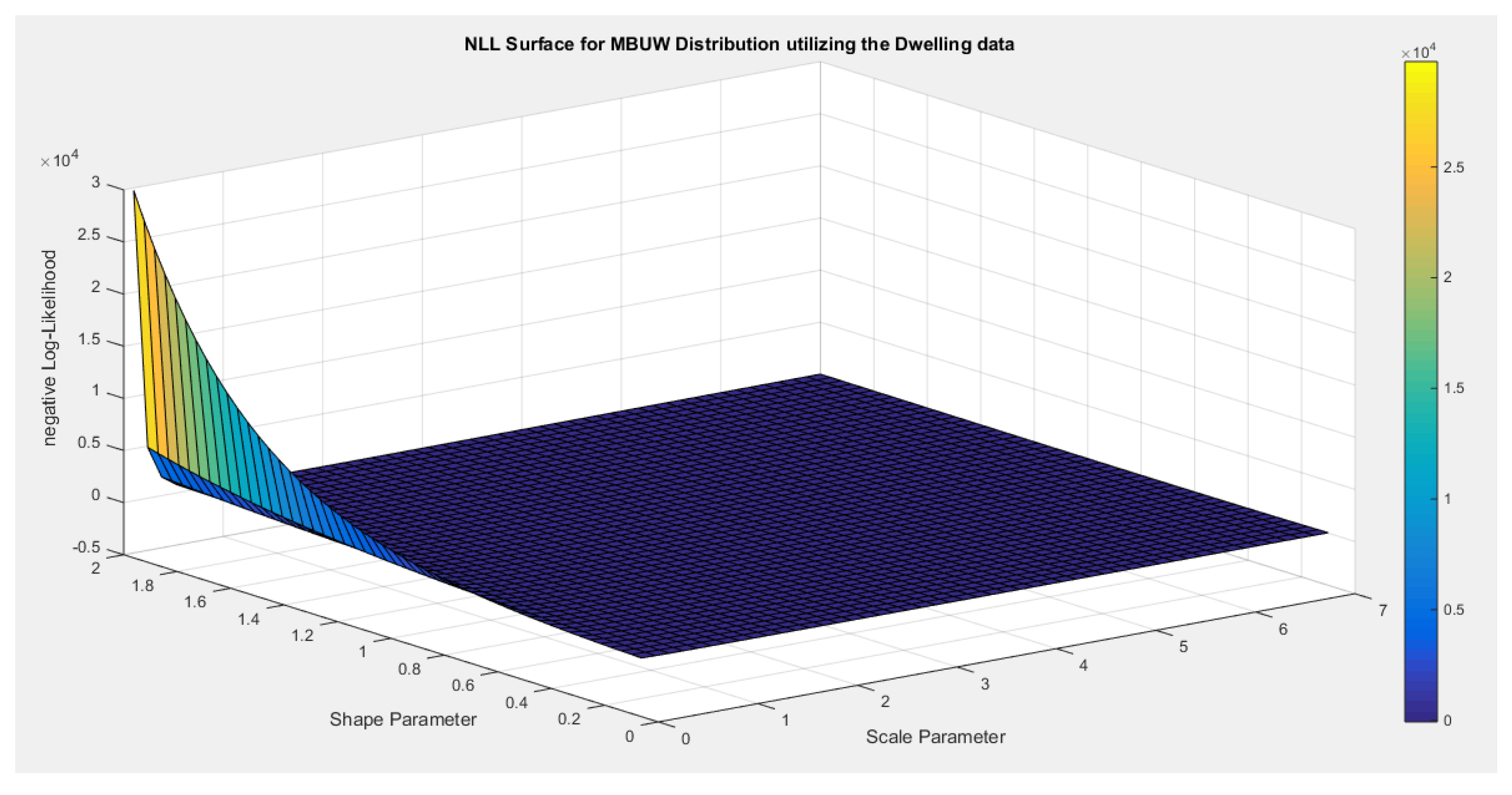
Figure 2.
shows a decreasing convex relationship between alpha and beta. The Nonlinear models for the time between failures dataset, with residual sum of squares (RSS), R^2 and root of mean square error(RMSE) are illustrated in the figure for each curve, high lightening that the exponenetial is the best model followed by the reciprocal model then the polynomial ( quadratic) model.
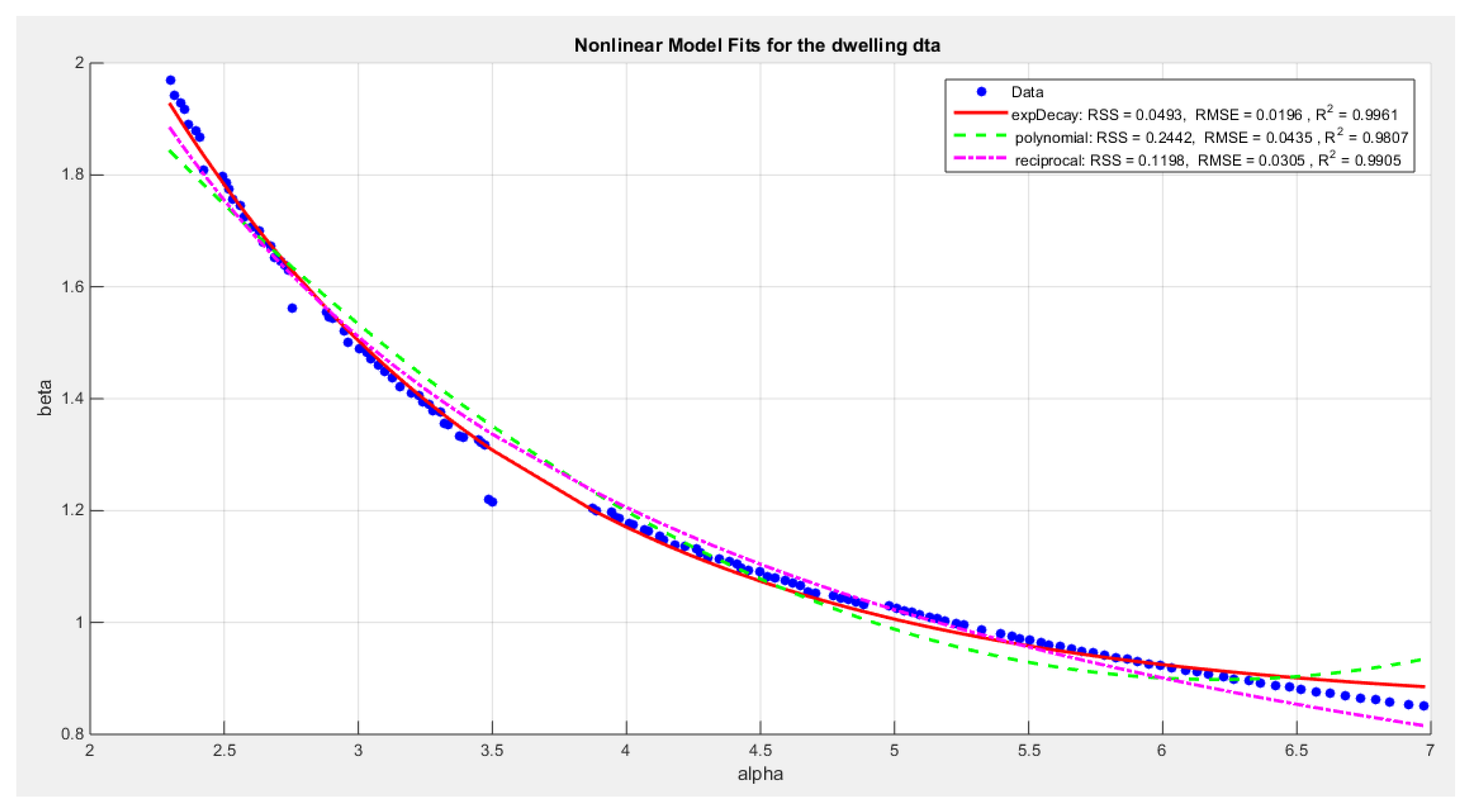
Figure 3.
negative likelihood surface using the Quality of support network dataset.
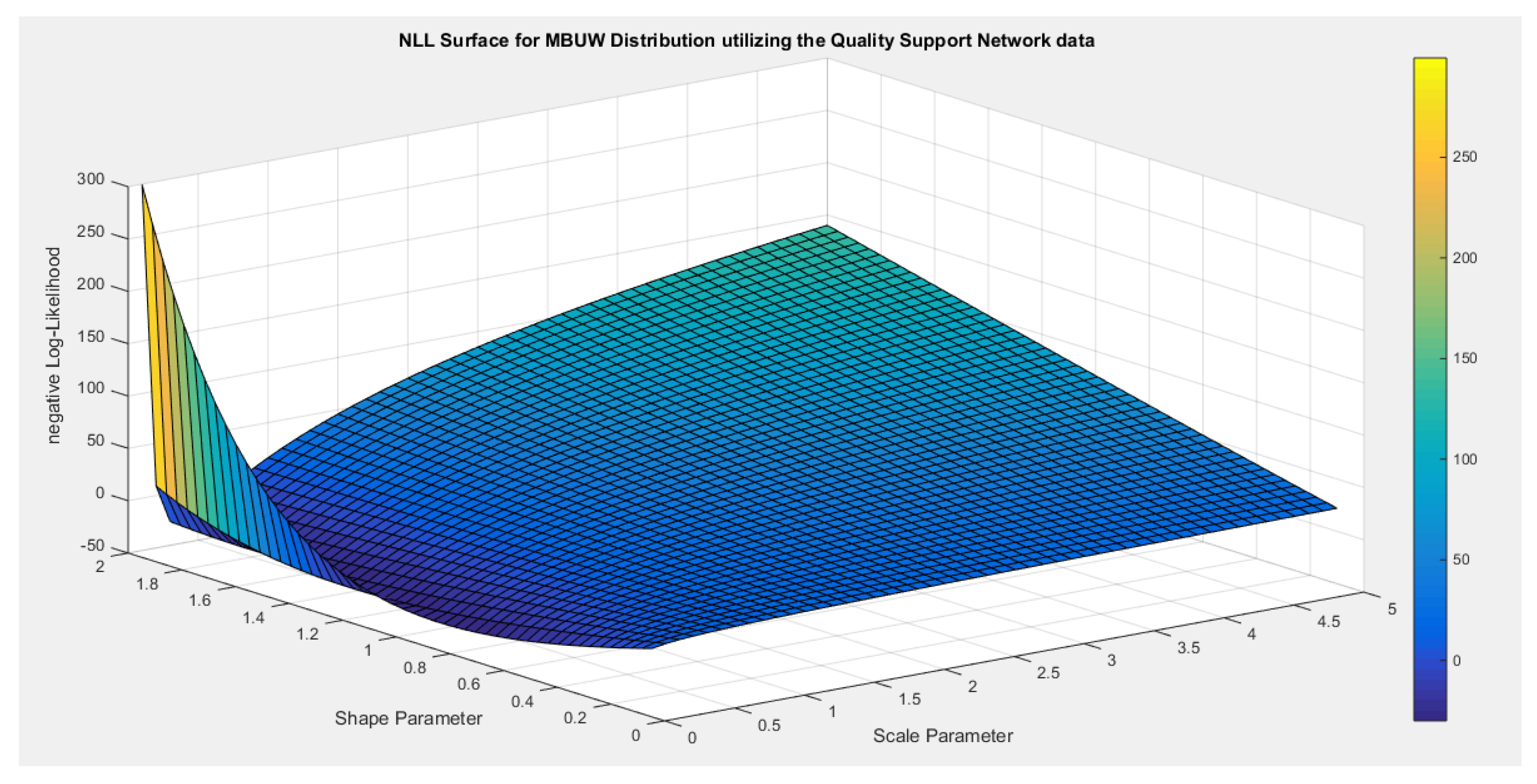
Figure 4.
shows the increasing linear relationship between the alpha and the beta parameter, with RSS=0.0029, R^2=0.9977 and RMSE=0.014 shown in the figure.
Figure 4.
shows the increasing linear relationship between the alpha and the beta parameter, with RSS=0.0029, R^2=0.9977 and RMSE=0.014 shown in the figure.
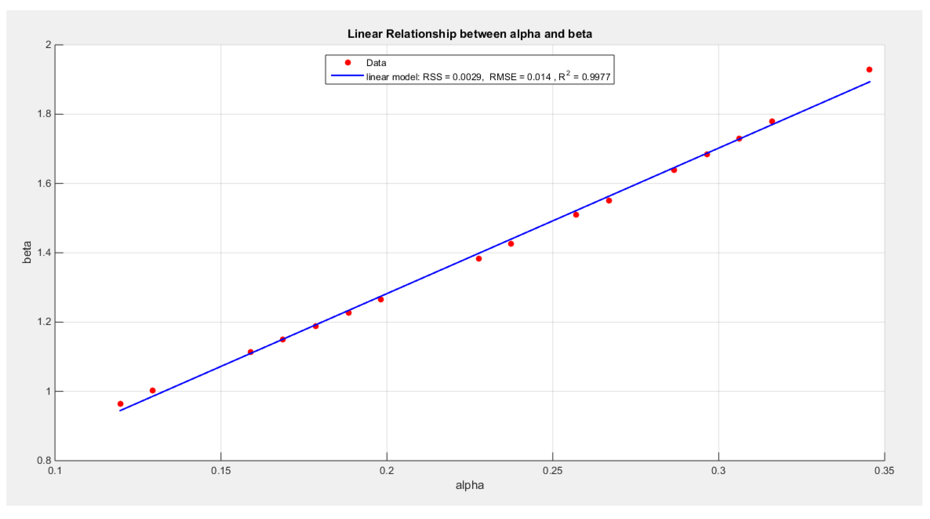
Figure 7.
negative likelihood surface using the Voter dataset.
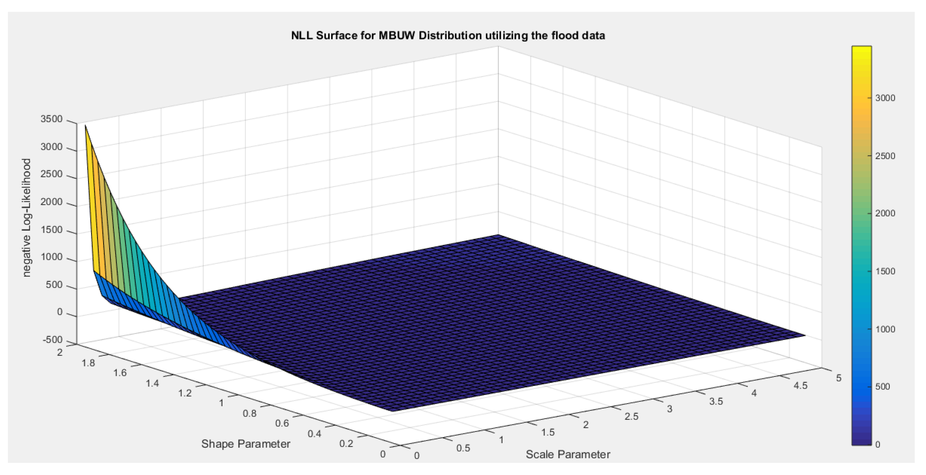
Figure 8.
shows a decreasing convex relationship between alpha and beta. The Nonlinear models for the flood dataset, with residual sum of squares (RSS), R^2 and root of mean square error(RMSE) are illustrated in the figure for each curve, high lightening that the exponenetial is the best model followed by the polynomial( quadratic) then the reciprocal model.
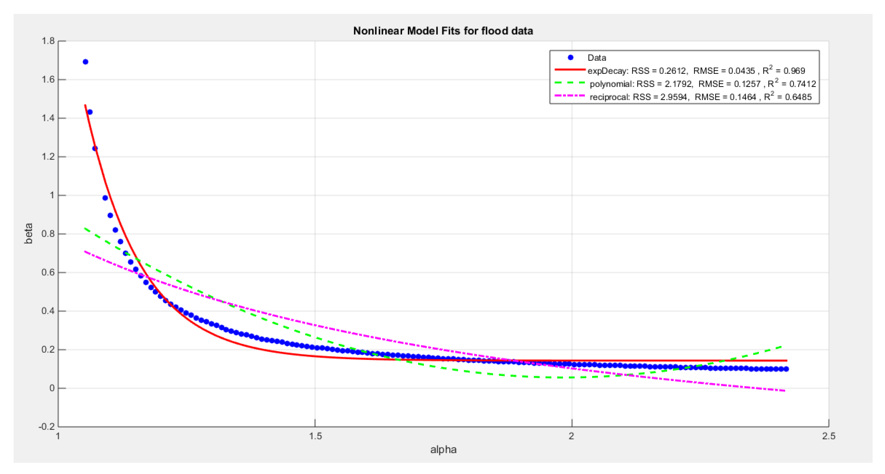
Figure 9.
negative likelihood surface using the Voter dataset.
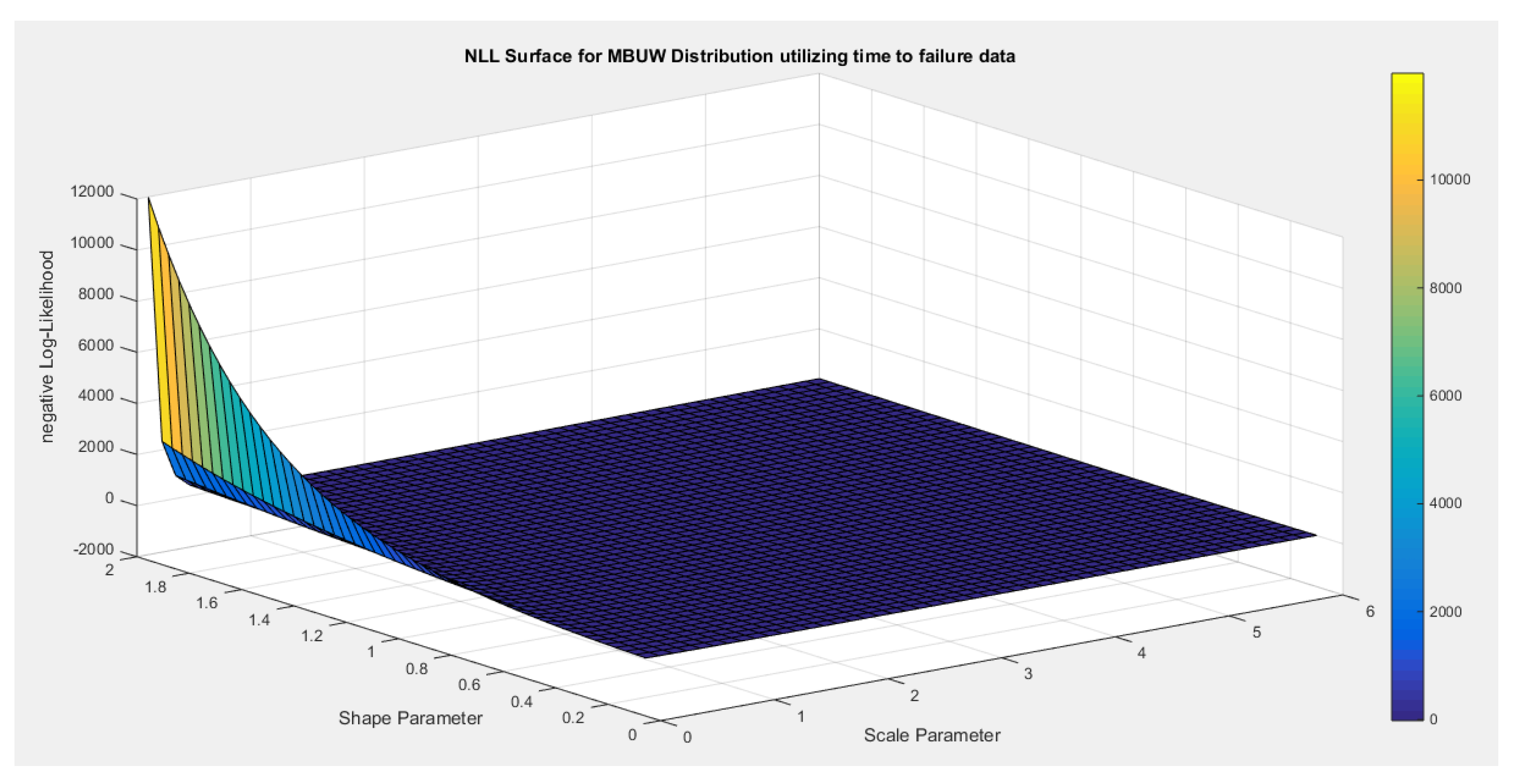
Figure 10.
shows a decreasing convex relationship between alpha and beta. The Nonlinear models for the time between failures dataset, with residual sum of squares (RSS), R^2 and root of mean square error(RMSE) are illustrated in the figure for each curve, high lightening that the exponenetial is the best model followed by the reciprocal model then the polynomial (quadratic).
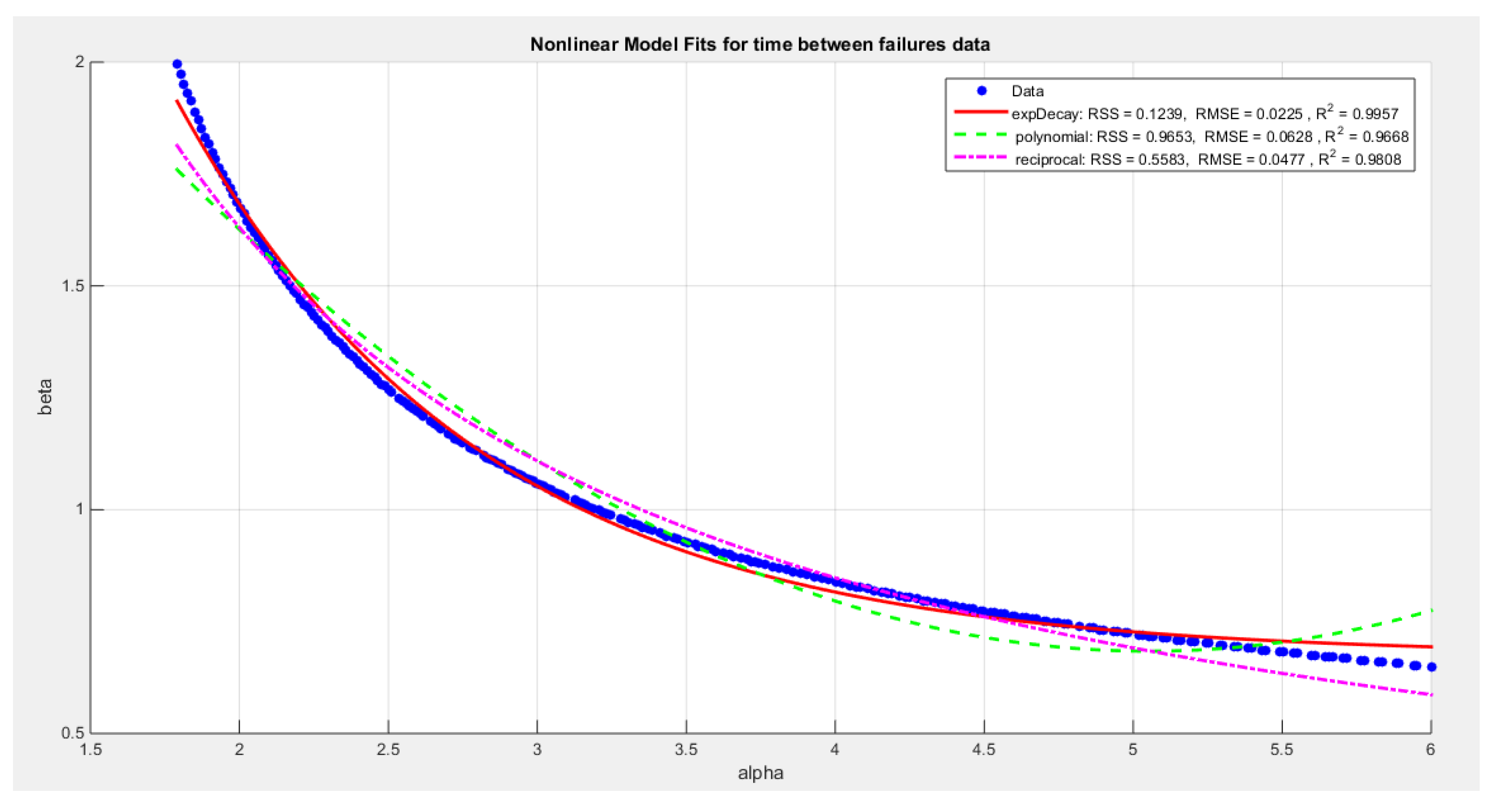
Figure 11.
negative likelihood surface using the Voter dataset.
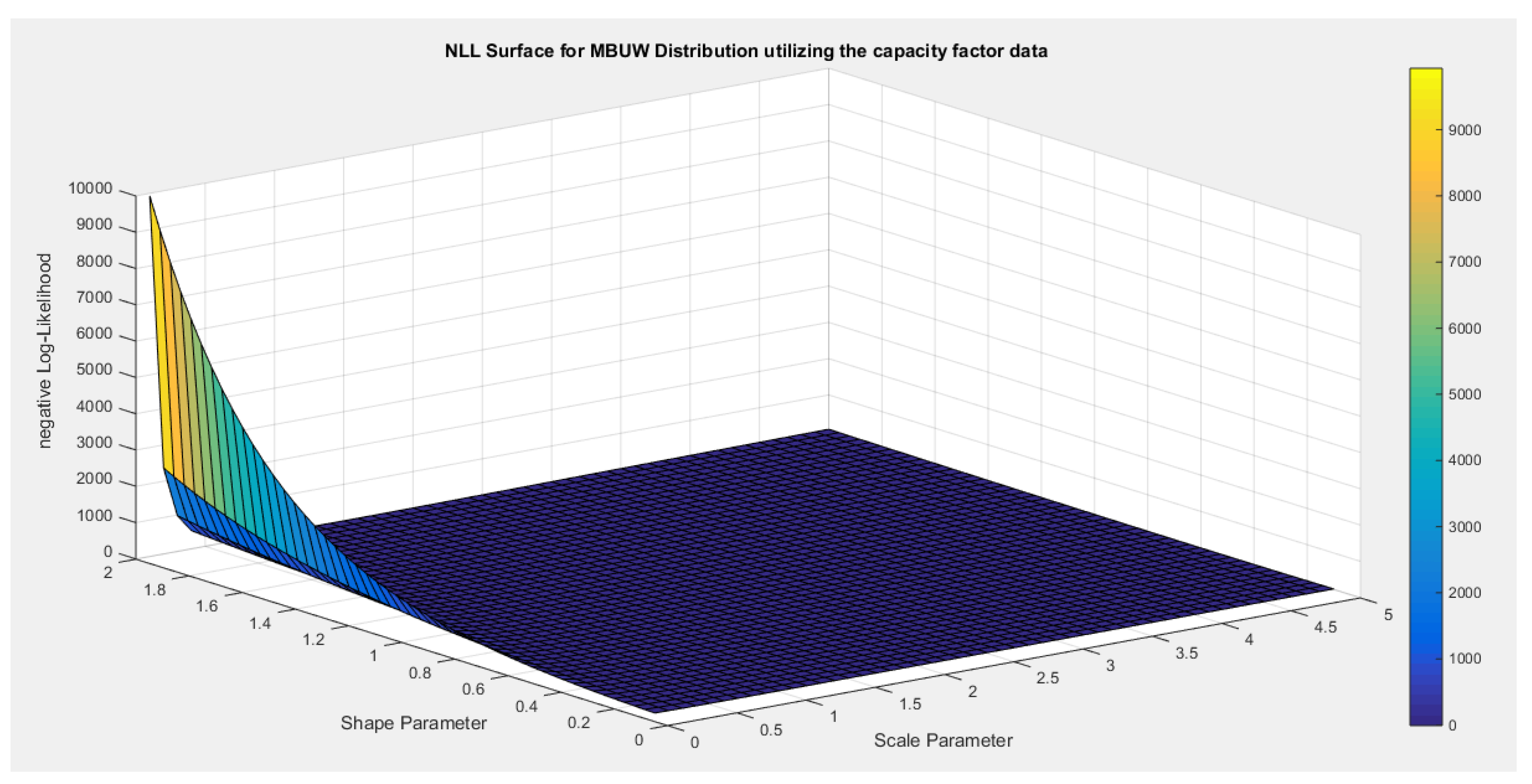
Figure 12.
shows a decreasing convex relationship between alpha and beta. The Nonlinear models for the capacity factor dataset, with residual sum of squares (RSS), R^2 and root of mean square error(RMSE) are illustrated in the figure for each curve, high lightening that the exponential is the best model followed by the reciprocal model then the polynomial ( quadratic).
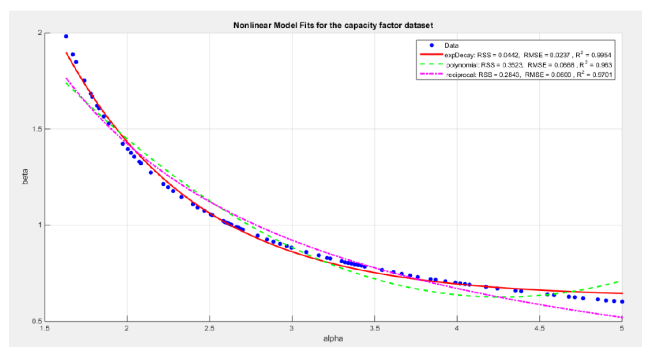
Figure 13.
shows the CDF on the right and QQ plot on the left for the Dwelling dataset before and after correction.
Figure 13.
shows the CDF on the right and QQ plot on the left for the Dwelling dataset before and after correction.
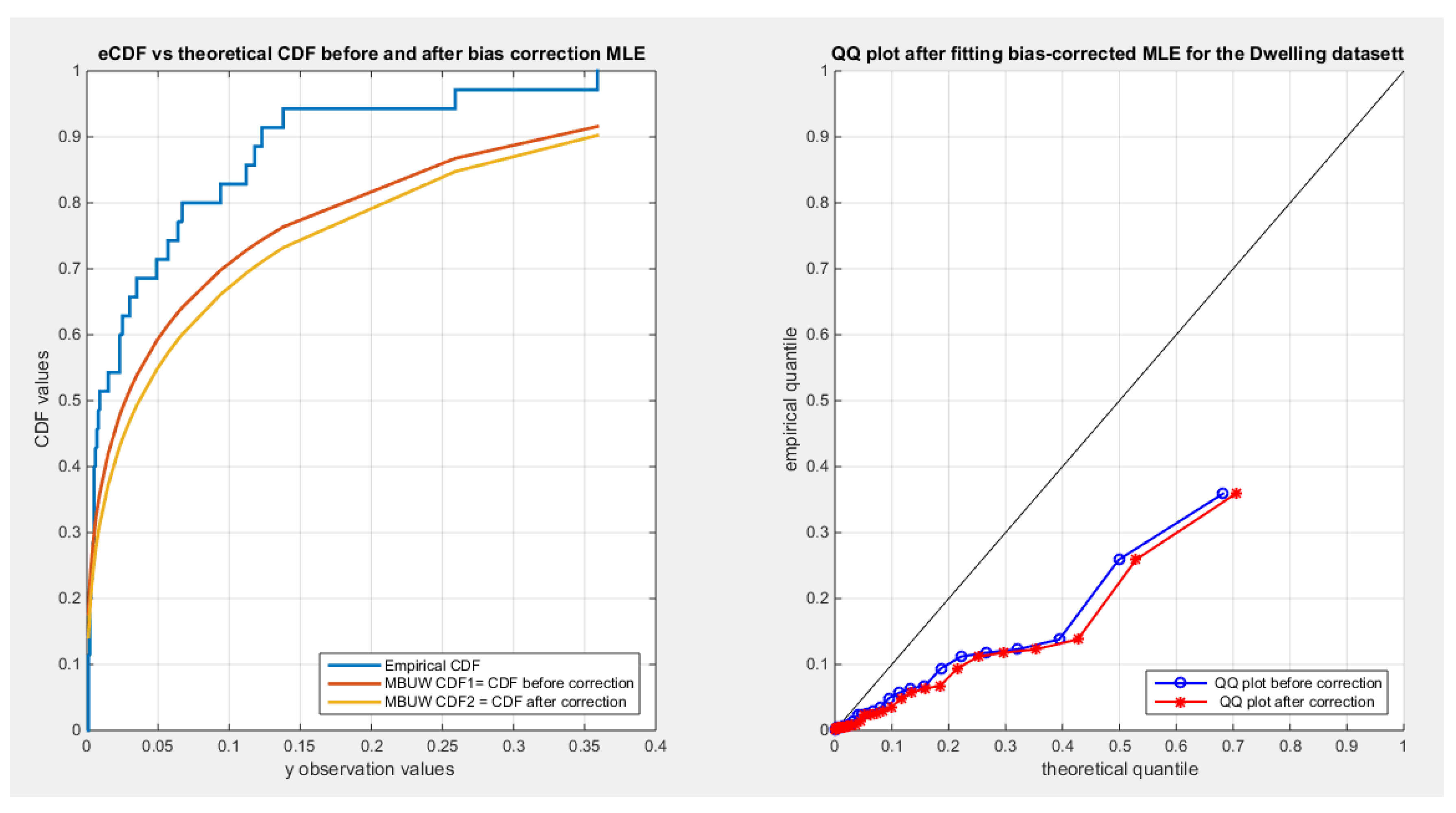
Figure 14.
shows the CDF on the right and QQ plot on the left for the time between failures dataset before and after correction.
Figure 14.
shows the CDF on the right and QQ plot on the left for the time between failures dataset before and after correction.
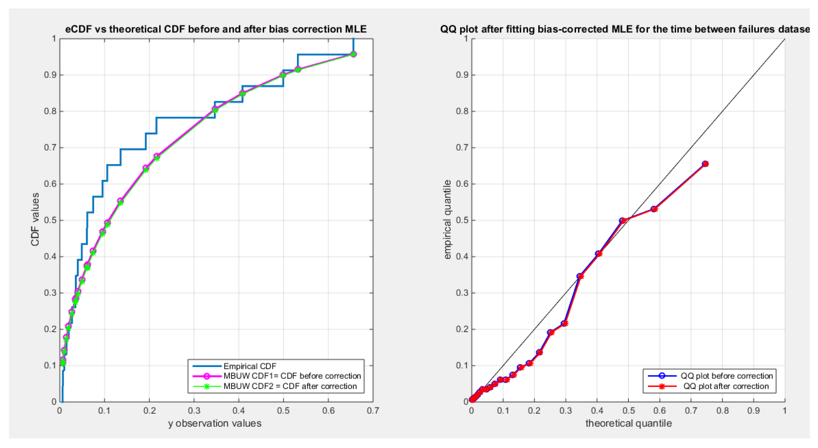
Figure 15.
shows the CDF on the right and QQ plot on the left for the factors affecting unit capacity dataset before and after correction.
Figure 15.
shows the CDF on the right and QQ plot on the left for the factors affecting unit capacity dataset before and after correction.
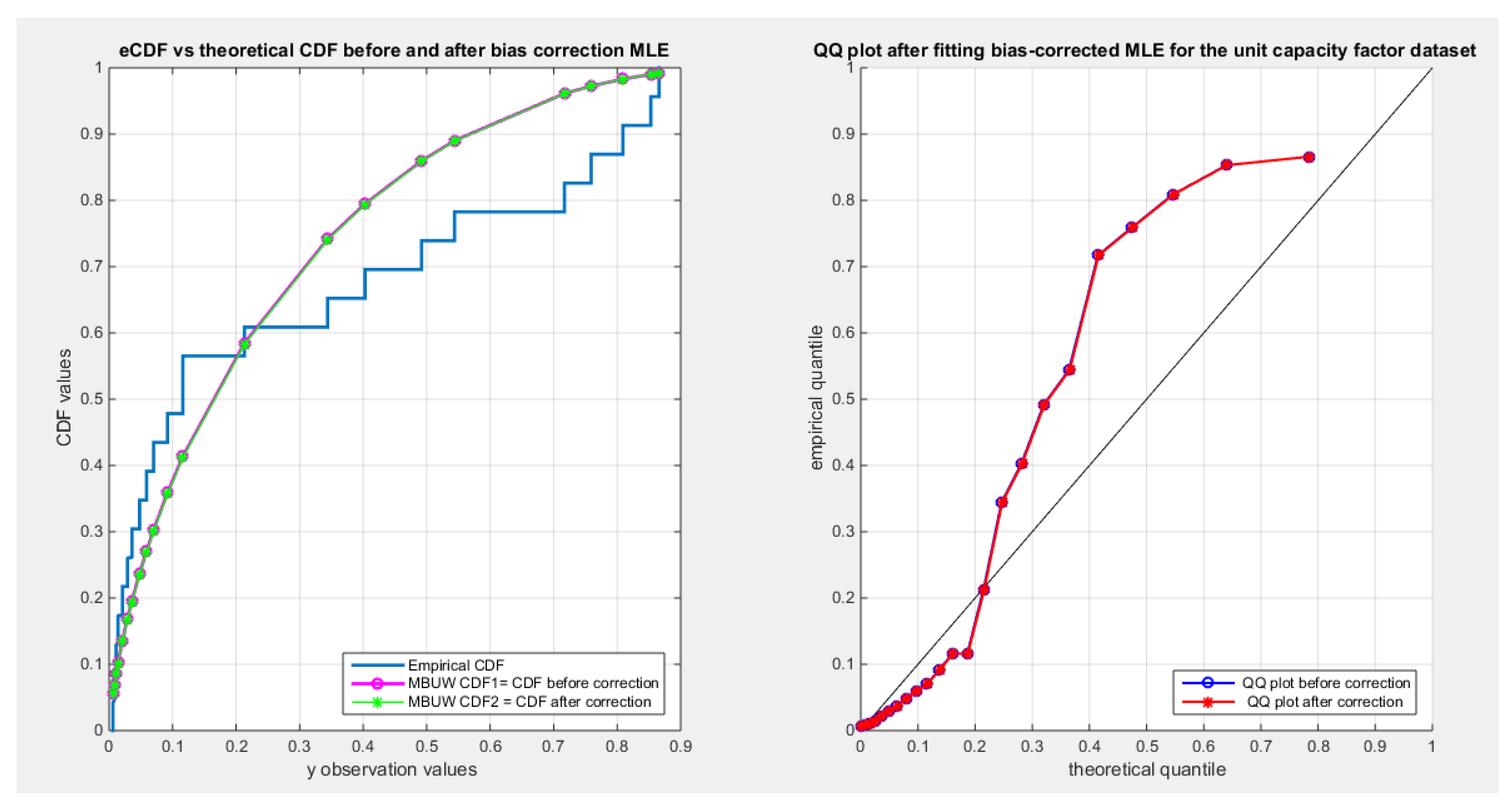

Table 1.
the results of the 3 nonlinear model using the dwelling data.
| metric | Exponential decay | Quadratic-polynomial | Reciprocal |
| Alpha | 2.7988 (2.7286,2.869) |
2.72268 (2.6602,2.7935) |
2.8707 (2.7969,2.9444) |
| Beta | 1.6045 (1.5669,1.6421) |
1.6461 (1.6175,1.6748) |
1.5659 (1.5331,1.5987) |
| Var (SE) alpha |
0.0449 (0.0358) |
0.0405 (0.034) |
0.0496 (0.0376) |
| Var (SE) beta |
0.0129 (0.0192) |
0.0075 (0.0146) |
0.0098 (0.0167) |
| nLL | -74.2925 | -74.2925 | -74.2925 |
| KS | 0.1794 | 0.1794 | 0.1794 |
| AD | 2.3889 | 2.3889 | 2.3889 |
| CVM | 0.3966 | 0.3966 | 0.3966 |
| AIC | -144.585 | -144.585 | -144.585 |
| CAIC | -144.21 | -144.21 | -144.21 |
| BIC | -141.4743 | -141.4743 | -141.4743 |
| HQIC | -3.5422 | -3.5422 | -3.5422 |
| Ho | Fail to reject | Fail to reject | Fail to reject |
| P-value (KS-test) |
0.186 | 0.186 | 0.186 |
Table 2.
results from second dataset.
| Alpha & CI | Beta & CI | Var(alpha) & SE | Var(beta) & SE | H0&p(KS) |
| 0.0558 (0.0492,0.0624) |
0.6763 (0.6486,0.704) |
0.00023 (0.0034) |
0.004 (0.0141) |
Fail to reject (p=0.8235) |
Table 3.
results from second dataset (continuation).
| AIC | CAIC | BIC | HQIC | KS | AD | CVM | nLL |
| -55.734 | -55.0281 | -53.7425 | -2.4048 | 0.1061 | 0.452 | 0.0803 | -29.867 |
Table 4.
the results of the 2 nonlinear models using the voter data.
| metric | Power law model | Quadratic-polynomial model |
| Alpha | 0.483 (0.4661,0.4998) |
0.4297 (0.4118,0.4471) |
| Beta | 1. 0563 (1.0007,1. 112) |
0.9014 (0.8509,0.9519) |
| Var(SE) alpha |
0.0028 (0.0086) |
0.0031 (0.009) |
| Var(SE) beta |
0.0306 (0.0284) |
0.0252 (0.0258) |
| nLL | -22.0671 | -22.0688 |
| KS | 0.1395 | 0.1364 |
| AD | 1.3657 | 1.3262 |
| CVM | 0.2295 | 0.2193 |
| AIC | -40.1342 | -40.1377 |
| CAIC | -39.7914 | -39.7948 |
| BIC | -36.859 | -36.8625 |
| HQIC | -1.0229 | -1.0231 |
| Ho = 0 | Fail to reject | Fail to reject |
| P-value (KS-test) |
0.412 | 0.4401 |
Table 5.
the results of the 3 nonlinear models using the flood data.
| metric | Exponential decay | Quadratic-polynomial | Reciprocal |
| Alpha | 1.0712 (1.0114 , 1.1311) |
1.1312 (1.0179 , 1.2444) |
1.1575 (1.02 , 1.295) |
| Beta | 1.2591 (0.6507,1.8675) |
0.7027 (0.5309,0.8744) |
0.5921 (0.4542,0.7301) |
| Var(SE) alpha |
0.0186 (0.0305) |
0.0668 (0.0578) |
0.0984 (0.0702) |
| Var(SE) beta |
1.9269 (0.3104) |
0.1535 (0.0876) |
0.0991 (0.0704) |
| nLL | -6.4617 | -6.4617 | -6.4617 |
| KS | 0.3202 | 0.3202 | 0.3202 |
| AD | 2.7563 | 2.7563 | 2.7563 |
| CVM | 0.531 | 0.531 | 0.531 |
| AIC | -8.9233 | -8.9233 | -8.9233 |
| CAIC | -8.2174 | -8.2174 | -8.2174 |
| BIC | -6.9319 | -6.9319 | -6.9319 |
| HQIC | 0.657 | 0.657 | 0.657 |
| Ho | Fail to reject | Fail to reject | Fail to reject |
| P-value (KS-test) |
0.0253 | 0.0253 | 0.0253 |
Table 6.
the results of the 3 nonlinear models using the time between failures data.
| metric | Exponential decay | Quadratic-polynomial | Reciprocal |
| Alpha | 1.977 (1.906 , 2.048 ) |
2.105 (2.0224 , 2.1875) |
2.141 (2.0551 , 2.2269 ) |
| Beta | 1.7062 (1.6343,1.778) |
1.5624 (1.5132 , 1.6116 ) |
1.5276 (1.4689 , 1.5853 ) |
| Var (SE) alpha |
0.0302 (0.0362) |
0.0408 (0.0421) |
0.0442 (0.0438) |
| Var (SE) beta |
0.0309 (0.0367) |
0.0145 (0.0251) |
0.0206 (0.0299) |
| nLL | -19.931 | -19.931 | -19.931 |
| KS | 0.1584 | 0.1584 | 0.1584 |
| AD | 0.6703 | 0.6703 | 0.6703 |
| CVM | 0.1253 | 0.1253 | 0.1253 |
| AIC | -35.862 | -35.862 | -35.862 |
| CORR AIC |
-35.262 | -35.262 | -35.262 |
| BIC | -33.591 | -33.591 | -33.591 |
| HQIC | -1.4134 | -1.4134 | -1.4134 |
| Ho = 0 | Fail to reject | Fail to reject | Fail to reject |
| P-value (KS-test) |
0.5575 | 0.5575 | 0.5575 |
Table 7.
the results of the 3 nonlinear models using the capacity data.
| metric | Exponential decay | Quadratic-polynomial | Reciprocal |
| Alpha | 1.7729 (1.7086 , 1.8373 ) |
1.8767 (1.8018 , 1.9516) |
1.9217 (1.8421 , 2.0012 ) |
| Beta | 1.6943 (1.6098,1.7787) |
1.5412 (1.5984 , 1.484 ) |
1.4853 (1.4205 , 1.5502 ) |
| Var (SE) alpha |
0.0248 (0.0328) |
0.0336 (0.0382) |
0.0379 (0.0406) |
| Var (SE) beta |
0.0427 (0.0431) |
0.0196 (0.0292) |
0.0252 (0.0331) |
| nLL | -7.6079 | -7.6079 | -7.6079 |
| KS | 0.1518 | 0.1518 | 0.1518 |
| AD | 1.9075 | 1.9075 | 1.9075 |
| CVM | 0.2033 | 0.2033 | 0.2033 |
| AIC | -11.2158 | -11.2158 | -11.2158 |
| CAIC | -10.6158 | -10.6158 | -10.6158 |
| BIC | -8.9448 | -8.9448 | -8.9448 |
| HQIC | 0.5128 | 0.5128 | 0.5128 |
| Ho = 0 | Fail to reject | Fail to reject | Fail to reject |
| P-value (KS-test) |
0.4074 | 0.4074 | 0.4074 |
Table 8.
the bias and values of parameters before and after correction.
| Dwelling | |||
| Before correction | bias | After correction | |
| alpha | 2.7268 | -0.707 | 2.7975 |
| Beta | 1.6461 | 0.1273 | 1.5188 |
| Time between failure | |||
| alpha | 2.105 | -0.000656 | 2.1057 |
| Beta | 1.5624 | 0.0171 | 1.5453 |
| Factors affecting unit capacity | |||
| Alpha | 1.8767 | 0.000459 | 1.8762 |
| beta | 1.5412 | 0.0046 | 1.5366 |
Table 9.
Metrics after applying bias-corrected MLE on the mentioned datasets.
| Metrics | Dwellings | Time between failures | Factors affecting unit capacity | |||
| nLL | -74.0169 | -19.9277 | -7.6076 | |||
| AIC | -144.0338 | -35.8553 | -11.2153 | |||
| CAIC | -143.6588 | -35.2553 | -10.6153 | |||
| BIC | -14.9231 | -33.5843 | -8.9443 | |||
| HQIC | -3.5348 | -1.4131 | 0.5128 | |||
| KS | 0.2107 | 0.1643 | 0.1536 | |||
| AD | 3.2988 | 0.7135 | 1.9104 | |||
| CVM | 0.6162 | 0.1371 | 0.2051 | |||
| P(KS) | 0.0766 | 0.5072 | 0.4090 | |||
| Inverse of K matrix= Var-cov matrix |
0.0016 | -.00056 | 0.0021 | -.00064 | 0.0027 | -.00056 |
| -.00056 | .00082 | -.00064 | 0.0032 | -.00056 | 0.007 | |
Disclaimer/Publisher’s Note: The statements, opinions and data contained in all publications are solely those of the individual author(s) and contributor(s) and not of MDPI and/or the editor(s). MDPI and/or the editor(s) disclaim responsibility for any injury to people or property resulting from any ideas, methods, instructions or products referred to in the content. |
© 2025 by the authors. Licensee MDPI, Basel, Switzerland. This article is an open access article distributed under the terms and conditions of the Creative Commons Attribution (CC BY) license (http://creativecommons.org/licenses/by/4.0/).
Copyright: This open access article is published under a Creative Commons CC BY 4.0 license, which permit the free download, distribution, and reuse, provided that the author and preprint are cited in any reuse.


