
Submitted:
13 October 2025
Posted:
14 October 2025
You are already at the latest version
Abstract
The objective of this work is the development of a highly effective Wiener-Physically-Informed-Neural-Network (W-PINN) modeling methodology for systems and processes with highly nonlinear dynamic and highly nonlinear static behavior. This approach has two basic stages. The first stage estimates all the unknown linear dynamic modeling coefficients. With these estimates fixed, the second stage estimates all the unknown static coefficients in an artificial neural network (ANN) framework. When the ANN is a nonlinear function, as in this work, the fitted model is a nonlinear dynamic and nonlinear static structure. In a previous one stage, 60-minute forecast modeling case, the dynamic outputs (vij, where i = the subject number and j = the sample number) were estimated in Excel® for eleven (11) type 1, freely-living, diabetes data sets (cases) of approximately two weeks of data, yielding an average input-only sensor glucose concentration (SGC) validation fit () of 0.68. With these vij’s fixed, this new approach obtains final, two-stage (TS) W-PINN, 60-minute forecast fitted models, for each of the 11 cases, in two ways. One two-stage approach uses the JMP® ANN toolbox for second stage modeling and achieves an average input-only SGC of 0.74 and maximum of 0.84. The second two-stage approach uses a novel ANN methodology coded in Python® and achieves an average input-only SGC of 0.82 and maximum of 0.93. Incorporating bias correction, using current and past SGC residuals, the Python® estimator improved the average from 0.82 to 0.87 with the maximum still 0.93.
Keywords:
Block-oriented Modeling
; Forecast Modeling
; Forecast Control
; Free-living Data Collection
; Glucose Modeling
; Hammerstein Modeling
; Physically-Informed-Neural-Network
; Type 1 Diabetes
; Weiner Modeling
1. Introduction
Our objective is the extension of the Wiener-Physically-Informed-Neural-Network (W-PINN) approach developed by [1] to improve modeling effectiveness when processes (i.e., systems) are highly nonlinear. W-PINN is a two-step modeling methodology. In Step 1, p inputs enter and exit their own linear dynamic modeling structure. In Step 2, the p dynamic outputs enter a static modeling structure that outputs the fitted response. W-PINN effectively and accurately modeled a real industrial grain dryer, a batch process with first order (FO) dynamic behavior and simple (i.e., one input) linear regression static behavior [1]. [2] recently introduced the Theoretically-based Dynamic Regression (TDR) modeling approach to tie it to, and to distinguish it from, Dynamic Regression (DR) [3,4,5,6,7], a familiar lagged-based approach in several academic disciplines. More specifically, the core difference between TDR and DR is that TDR uses physically-based dynamic structures and DR uses lagged (i.e., empirically)-based structures. Thus, TDR is more parsimonious, physically interpretable, and exploitable than DR. However, with its limitation to first- and second-order linear dynamic structures, and its lack of connection to ANN, TDR can be viewed as a subclass of W-PINN.
[2] applied TDR in three (3) modeling cases. The first one modeled a subject’s weight (y) with the consumption of four nutrients (xi), i.e., four inputs. The fitted model is a first-order (FO), linear dynamic/quadratic static structure. The training rfit = 0.92 and the validation rfit = 0.91. The second case in [2] modeled the top tray temperature (y) of a pilot distillation column with nine (9) inputs (xi). It resulted in a complex second-order linear dynamic structure for each input and a simple FO multiple-input static regression function. The training rfit = 0.96, the validation rfit = 0.97, and the average testing rfit for nine (9) data sets over a three-year period equaled 0.84. The third case modeled the sensor glucose concentration (SGC) (y) of eleven (11) type 1 diabetes data sets using twelve (12) inputs in outpatient (free-living) data collection of two weeks. It also resulted in a complex second-order linear dynamic model structure for each input. However, the static structure is quite complex and limited this case to a first-order, multiple-input, static structure. For the second study, there was one process, the distillation column. In the SGC modeling study, each subject is a process, or system, and thus has its own one-week of training/one-week of validation results. For these eleven sets of results, the average for training and validation equaled 0.62 and 0.68, respectively.
Moreover, the objective of this work is the development of an effective W-PINN modeling approach for dynamic systems with highly complex static behavior. More specifically, using the Stage 1 SGC dynamic modeling results obtained by Rollins et al. (2025) [2], the objective of this work is to significantly increase using a novel, proposed, two-stage, W-PINN modeling approach.
The classical ANN approach is a one-box, empirical modeling methodology as illustrated in Fig. 1a. As shown, p measured xi inputs enter the ANN function, , an estimated (as denoted by “^”) empirical function with constant coefficients that are adjusted under some criterion, commonly least squares estimation, to maximize agreement (i.e., fit) between its modeled output, and its measured output, y (e.g., SGC), where is a pth dimensional vector of measured inputs. In Fig. 1a, can be a static function, e.g., a non-linear regression function, or a combined static and empirically dynamic function of lag variables, e.g., a Long- and Short-Term Memory (LSTM) [8, 9] function.
Phenomenologically dynamic and empirically static methodologies are illustrated in Figs. 1b (PINN [10]) and 1c (W-PINN, [1]). [10] named their methodology “physically-informed-neural-network” (PINN). The critical difference between Fig. 1a (classical ANN) and Figs. 1b and 1c are the number of stages. Figure 1a has one stage for static and dynamic structures, and the two-stage methods in Figs. 1b and 1c have one stage for static structures and one stage for dynamic structures. The PINN dynamic block is not restricted to linear dynamic structures as it is for W-PINN. However, nonlinear dynamic behavior is modeled when the dynamic outputs of W-PINN (i.e., ) are passed through . A critical advantage of W-PINN over PINN is that each input has its own dynamic model structure, as illustrated by comparing Figs. 1b and 1c.
The next section, Section 2, describes the W-PINN methodology fundamentally and mathematically. The theoretical structure of a general and complete second-order dynamic structure is first given in Section 2.1 as differential equation and then transformed to its discrete-time version using backward difference derivatives. It then gives the explicit equation for , where “t” is the sampling time. Section 2.2 gives important Stage 1 details and results to assist in the understanding of the Stage 2 methodology. Section 2.3 describes the JMP® and Python® Stage 2 methodologies. Section 2.4 give the mathematical details of Model 1 (input only model), Model 2 (input-output) and Model 1-2, a combination of the strengths of Models 1 and 2. Section 2.5 gives the forecast model structure, i.e., the structure for Finally, Section 2.6 gives the information and equations for the summary statistics.
Section 3 gives a table with all the numerical results for the three modeling methods. It also gives Model 1, Model 2 and Model 1-2 graphical results for the best fitting Stage 2 subject, Subject 2. For all three models, their validation is 0.93. Section 4 gives a discussion of the results and Section 5 comments on work in progress and speculates on other possible future directions.
2. Materials and Methods
This section describes the two-step W-PINN methodology in detail. It also gives critical Stage 1 SGC modeling particulars used by [2] to obtain the posted on the website of the last author at https://drollins9.wixsite.com/derrickrollins. With both the and posted on this website, modelers have the option of using these data sets to build both stages or just the second stage, the aim of this work.
With the sampling rate, Δt, equal to 5 minutes, our SGC models are forecasting 12-steps (i.e., 60 minutes) into the future. The forecast nature of this work is an artifact of the data sets we are using and their application and, thus, not a necessity of the methodology. As described in [2], 12Δt is the estimated observable time it took for the manipulated variable (MV), exogenous insulin, to cause SGC to start decreasing after a bolus increase (or insulin injection). The 60-minute estimate was very consistent for the subjects in this clinical study as noted in [2].
The models that this work develops are for an unobservant, 60-minute, forecast monitoring scenario. “Unobservant” is meant to convey the protocol that the person(s) determining insulin changes have no knowledge of the forecast () estimates. In addition, even though the authors of [2] worked diligently to obtain models that minimize pairwise correlation, we note that it is still significantly present. Thus, for this reason, this work is best understood as an unobservant monitoring application and not applicable to closed-loop control.
2.1. W-PINN
Our W-PINN approach uses backward difference derivatives (BDD) to discretize second-order-plus-dead-time-plus-lead (SOPDTPL) (see [12]) theoretical dynamic systems, the only type used in this work, as given in Eq. 1, below. The dynamic system does not have to be initially at a steady state for our W-PINN modeling methodology since the initial conditions are also estimated. Note that, Eq. 1 is the expression for each of the p-inputs.
with
where and for i = 1, …, p, xi(t) is the value of the ith input variable at t, and vi(t) is the value of the ith output variable at t, in the units of xi, y(t) is the output variable in its units at t, means the expected value (i.e., true mean) of y(t), is the true output (gain) function of V(t), the vector of the vi(t)’s. When is a nonlinear function of V(t), as in the ANN (i.e., W-PINN) case, Eqs. 1 and 2, taken together, have a Wiener block-oriented structure [11], as shown in Fig. 1c.
The lead term is the first term on the right side of the equal sign in Eq.1. This term tends to "speed up" the response and provides what the process modeling and control community has termed "numerator dynamics" [11,12,13]. [11] developed a second-order, multiple-input, single-output, discrete-time, nonlinear Wiener dynamic approach using BDD based on Eq. 1. More specifically, using BDD approximation applied to a sampling interval of Δt, an approximate discrete-time form of Eq. 1 is
with
such that to satisfy the unity gain constraint. From Eq. 3 with
After obtaining for each input i, the modeled output value, at time t, is determined by entering these results into , a static ANN in this application, i.e.,
2.2. Stage 1 Modeling Method
This subsection gives important Stage 1 details and results to assist in the understanding of the Stage 2 methodology. While missing output (i.e., SGC) measurements are acceptable, missing input values are not for discrete-time modeling. Activity tracker data were the only missing input data. These missing values were estimated by averaging the two values on both sides of a gap and filling in the gap with this value. Some gaps were several hours long. Cross-validation [6] was used to guard against overfitting, with the first week as the training (Tr) data set, and the second week as the validation (Val) data set.
In Stage 1, all inputs were first modeled separately on their own Excel® worksheet with a first-order linear regression static function. For each case, insulin was modeled first. The estimated deadtime, i.e., was set at 60 minutes and was varied one Δt forwards and backwards at a time to find the value that gave the best fit. For all the inputs, the estimate of θMV, was determined to be 60 minutes, i.e., 12 Δt. The food variables were the only ones with announcements, and the carbohydrate input was the only one found to have a deadtime less than . The “time of day” input has no deadtime, and the dead time for all other inputs was except for fats that had deadtimes that were much larger than as determined by model estimation. After determining the dynamic coefficient estimates for each input (i.e., Eqs. 4 to 6), these values were copied to an Excel® worksheet as the dynamic structure starting values for fitting the SOPDTPL dynamic, and first-order static, multiple-input model (i.e., Eq. 10). With as a first-order multiple linear regression static function, for Stage 2 was determined.
2.3. Stage 2 Model Development Modeling Methods
The objective of this work is the development, evaluation, and comparison of two, Stage 2, W-PINN modeling approaches using from Stage 1 to obtain for each of the eleven data sets for the two approaches. The first approach uses the JMP® ANN toolbox to approximately find the smallest SSE (i.e., SSR) by fitting many cases and selecting the best one. The second approach is our newly developed, confidential, ANN structure that is coded using Python®. As Section 3 will show, both approaches significantly improved fit in comparison to as a first-order linear regression function.
2.4. Three Input Models
We developed three types of input model structures for this application. The first one we call the “input only model” or “Model 1.” All the inputs in this structure have a deadtime except for announcement inputs that can have deadtimes less than like carbohydrates, equal to like proteins, greater than like fats, and zero like time of day, as mentioned above.
The second one we call the “input-output model” or “Model 2.” It combines the input-only structure of Model 1 (i.e., Eq. 10) with a model of weighted residuals, a minimum of distance in the past (note that, this is model building and not model forecasting), as shown in Eq. 11 below (see [11] for the derivation).
Equation 11 has no value if any residual is not determinable due to missing output measurements. Thus, unlike Model 1, which has estimates for all t since it uses only input data, Model 2 will not have an estimate when an output value is missing.
The final model, Model 1-2, is a combination of the strengths of Models 1 and 2. More specifically, for Model 1-2,
2.5. Forecast Structures
Equation 10, , is the fitted structure for Model 1, i.e., estimate of the output, , at the current time, t. There are no missing input values in Eq. 10. This is why missing armband data had to be estimated. In addition, non-announcement input values to obtain Eq. 10 must be at least a distance of in the past. This requirement is because the model developed input lag must be the same as the forecast input lag, i.e., at t, for forecasting a distance into the future.
After obtaining , its transformation into the kΔt forecast form, i.e., the online version, is given by Eq. 13 below:
where, from Eq. 7, with t = t + kΔt,
Note that, if k = 12 and Δt = 5 minutes, the Eq. 14 model is forecasting 60 minutes into the future. Thus, all the non-announcement inputs must have, i.e., use, a model building and forecast prediction dead time of at least 60 minutes.
2.6. Statistical Analyses
The first, and most important, modeling statistic is rfit (which is bounded between -1 and 1), the fitted correlation of the measured SGC, , and the fitted SGC, , and given in Eq. 15 below.
where n is the number of samples in the set and the bar above a statistic means that it is its sample mean value. The equations to determine AAD and AD are, respectively,
The equation for SSE (i.e., SSR, the sum of squared residuals), the more common name and used by JMP®, is
3. Results
Training and Validation Stage 1 and Stage 2 summary statistics for the eleven subjects are given in Table 1. All the results are rfit unless indicated otherwise. Recalling that, each subject has a fixed that was determined in Stage 1 using the first-order static structure as given in Eq. 19, below:
As shown in Table 1, Stage 1, Model 1, rfit,val results varied from 0.59 to 0.77, with a mean of 0.68. Moreover, Stage 2, Model 1, rfit,val results improved significantly over the Stage 1 results for both ANN approaches. As shown, JMP® Stage 2, Model 1, rfit,val results varied from 0.60 to 0.85, with a mean of 0.74. However, Python® Stage 2, Model 1, rfit,val results are significantly better than JMP®, varying from 0.72 to 0.93, with a mean of 0.82. As a result, Model 2 training and validation results, and Models 1-2 validation results are given in Table 1 for Python® only. From Model 1 to Model 2, the Python® mean rfit,val increased from 0.82 to 0.87, the minimum from 0.72 to 0.80, and the maximum of 0.93 did not change. In summary, Python® Stage 2 results improved considerably over Stage 1 results and are significantly better than JMP® Stage 2 results.
Graphical Python® Stage 2 fitted and measured SGC results for Subject 2 (the best case) are given (i.e., plotted) in Figs. 2 to 4. Figure 2 is Model 1 training and validation. Figure 3 is Model 2 training and validation. Figure 4 plots are the combined validation results, with Model 1 plotted when there is no output data, and Model 2 is plotted when there is output data, i.e., the Model 1-2 validation plot. The Model 1-2 plots are associated with the results in the last three columns in Table 1. Figure 3 shows excellent fit of Model 2 and the highly realistic behavior of Model 1 when Model 2 results are not possible because of missing SGC data (see Eq. 11).
4. Discussion
In this study, two physically-based virtual forecasting sensor approaches were developed for obtaining the value of the response variable, SGC, a θMV time distance in the future, for a two-stage forecast modeling application. The first stage, a physically (i.e., theoretical) based dynamic modeling approach [11] estimates the physically interpretable dynamic parameters from the measured inputs (xi’s) with multiple physical constraints to obtain dynamic outputs (vi’s). The vi’s are the inputs to the second stage, a static ANN structure. For the first method, this structure was determined by using the ANN toolbox in JMP®. For the second method, this structure was determined by using a confidential method that this work developed and coded using Python®. Both methods resulted in large average improvements over the Stage 1 results using a first-order linear regression static structure (see Table 1). In addition, a critical advantage of these two approaches is that the modeling is much easier and much less time-consuming than the 2nd order multiple linear regression (MLR) approach. We do note, however, that static behavior of these data sets is highly nonlinear. Thus, we strongly recommend ANN over MLR for the static model structure, i.e., Note that ANN modeling is just a particular class of multiple nonlinear regression. We also note that the MLR model was applied to Subject 11 to compare the performance with the ANN. The rfit,val had a modest improvement from Stage 1 alone, going from 0.74 to 0.79, but much less than the 0.85 obtained by P-ANN.
We were pleasantly surprised by the P-ANN achievements of Models 1, 2, and 1-2. Model 1 has two subjects over the rfit,val goal of 0.90 and a mean of 0.82. Model 2 has four subjects meeting or exceeding the rfit,val goal and a significant increase in the mean rfit,val of 0.87. The combined Model 1 and Model 2 approach, i.e., Models 1-2, had essentially the same summary statistics results as Model 2, as shown in Table 1. Thus, combining Models 1 and 2, to have continuous forecasting without missing fits did not adversely affect rfit,val relative to Model 2, which had missing fits due to missing SGC measurements.
5. Conclusions and Future Work
The W-PINN approach is particularly powerful because each input xi is dynamically transformed to its vi counterpart and is the input to a static ANN. The proposed two-stage W-PINN approach greatly improved the SGC model fit for eleven historical diabetes data sets. A one-stage W-PINN approach, in its evaluation stage, is the next step in this research.
During his time as a professor, the second author gained valuable insight into the limitations of empirical modeling through a real-world industrial application. A BS Chemical Engineering student, also pursuing an MS in Statistics, undertook a summer project at a leading Midwest chemical company, which was approved for her MS thesis. The project focused on developing a multivariate Statistical Process Control (SPC) monitoring methodology for a process line. Data were collected, and an SPC control chart was developed, resulting in an excellent model fit. However, when the process exceeded control limits, adjustments to the manipulated variable based on this model failed to restore control. A subsequent attempt with new data and a revised control chart, despite another excellent fit, similarly failed to correct deviations when applied in a feedback control scenario. This experience highlighted that the control chart, designed for monitoring, was unsuitable for feedback control due to its reliance on empirical correlation rather than cause-and-effect relationships. Empirical SGC modeling, which uses free-living data and non-physiological structures, faces similar limitations, as it cannot adequately capture cause-and-effect dynamics critical for model-based control applications like automatic forecast control. In contrast, physically-informed modeling, which integrates physiological information and structure with free-living data, offers inherent intelligence and robust structure for potentially developing effective models for control applications. Our W-PINN methodology proposed in this manuscript is approaching the goal for the diabetes data set, but more research and creative screening of inputs are needed to fully realize the goal for SGC closed-loop feedback control. In addition, this advancement relies on a dual hormone scenario; one to decrease SGC, i.e., insulin; and one to as effectively and safely increase SGC, possibly glucagon. Nonetheless, our proposed two-stage methodology has promise, it seems, for physically-based, highly nonlinear static, systems or processes.
Type 1 diabetes SGC modeling for monitoring can be effective (i.e., informative) using empirical or physically-informed dynamic modeling approaches. Closed-loop Type 1 SGC automatic control is inherently forecast automatic control because a change in MV, injected insulin, will take a time of θMV to start lowering SGC. For automatic closed-loop control, empirical dynamic modeling approaches are not likely to succeed because they lack a cause-and-effect relationship, unlike PINN approaches. Insulin is the process variable that is changed to keep SGC close to its set point, i.e., it is the manipulated variable (MV). For a control system to do this well in a forecast feedback control scheme, the controlled variable, must be accurately estimated. An empirical method could possibly control online accurately if the correlation structure remains the same as it was when the model was developed. However, it is not possible for the correlation structure of an empirical forecast modeling approach in this context to remain intact, i.e., fixed, in online forecast feedback control because the correlation structure changes each time the controller signal to the manipulated variable is transmitted. Thus, it is prudent to restrict free-living empirical modeling to monitoring open-loop processes but not to make decisions on how much to change a manipulated variable to make changes in the control variable.
There are several challenges of the data sets used in this work. First, they are nearly a decade and a half old, and SGC technology has advanced considerably, particularly in terms of missing and lost data. Secondly, wearable technology have advanced considerably in reliability, measured sensor technology such as heart rate, as well as in data management. In addition, there are advancements in ways to get accurate consumption of food nutrients. Thus, one (distant) future goal is to evaluate W-PINN using data generated by current technology.
Supplementary Materials
The data sets are available to the public on the website of the corresponding author at https://drollins9.wixsite.com/derrickrollins.
Author Contributions
For research articles with several authors, a short paragraph specifying their individual contributions must be provided. The following statements should be used “Conceptualization, D.R. and D.H.; methodology, D.R. S.W. and D.H.; software, D.H. S.W. M.L. and Y.G.; validation, D.H., S.W. Y.G. and D.R.; formal analysis, D.R. and D.H.; investigation, D.H.; resources, D.R., M.L. and D.H.; data curation, D.H. S.W. and J.O.; writing—original draft preparation, D.H.; writing—review and editing, D.R. Y.G. and J.O.; visualization, D.H.; supervision, D.R.; project administration, D.R.; funding acquisition, M.L. All authors have read and agreed to the published version of the manuscript.
Funding
Not applicable as the work is part of the PhD research of Dillon G. Hurd with Dr. Rollins as Major Professor and Dr. Lamm as Co-Major Professor. Jacob Oyler was supported by the National Science Foundation under Grant No. EEC 1852125.
Institutional Review Board Statement
Not Applicable.
Informed Consent Statement
Not Applicable.
Data Availability Statement
The data sets are available to the public on the website of the corresponding author at https://drollins9.wixsite.com/derrickrollins.
Conflicts of Interest
The authors declare no conflicts of interest.
References
- Hurd, D.G.; Rollins, D.K. A Powerful AI Grain Moisture Sensor Approach with Demonstration on a Real In-Bin Grain Dryer. Smart Agricultural Technology 2025, 12, 101467. [Google Scholar] [CrossRef]
- Rollins, D.K.; Nilsen-Hamilton, M.; Kreienbrink, K.; Wolfe, S.; Hurd, D.; Oyler, J. Theoretically Based Dynamic Regression (TDR)—A New and Novel Regression Framework for Modeling Dynamic Behavior. Stats 2025, 8, 89. [Google Scholar] [CrossRef]
- Pefia, D. Measuring Influence in Dynamic Regression Models. Technometrics 1991, 33, 93–101. [Google Scholar] [CrossRef]
- Maekawa, K.; Yamamoto, T.; Takeuchi, Y.; Hatanaka, M. Estimation in Dynamic Regression with an Integrated Process. Journal of Statistical Planning and Inference 1996, 49, 279–303. [Google Scholar] [CrossRef]
- Pollock, D.S.G.; Pitta, E. The Misspecification of Dynamic Regression Models. Journal of Statistical Planning and Inference 1996, 49, 223–239. [Google Scholar] [CrossRef]
- Diniz, C.A.R.; Rodrigues, C.P. The Lag Length of a Dynamic Regression Model: A Comparative Study. AIP Conference Proceedings 2008, 1073, 150–156. [Google Scholar] [CrossRef]
- Costa, L.; Smith, J.Q.; Nichols, T. A Group Analysis Using the Multiregression Dynamic Models for fMRI Networked Time Series. Journal of Statistical Planning and Inference 2019, 198, 43–61. [Google Scholar] [CrossRef] [PubMed]
- Jaloli, M.; Cescon, M. Long-Term Prediction of Blood Glucose Levels in Type 1 Diabetes Using a CNN-LSTM-Based Deep Neural Network. J Diabetes Sci Technol 2023, 17, 1590–1601. [Google Scholar] [CrossRef] [PubMed]
- Kamalraj, R.; Neelakandan, S.; Ranjith Kumar, M.; Chandra Shekhar Rao, V.; Anand, R.; Singh, H. Interpretable Filter Based Convolutional Neural Network (IF-CNN) for Glucose Prediction and Classification Using PD-SS Algorithm. Measurement 2021, 183, 109804. [Google Scholar] [CrossRef]
- Guo, Y.; Cao, X.; Liu, B.; Gao, M. Solving Partial Differential Equations Using Deep Learning and Physical Constraints. Applied Sciences 2020, 10, 5917. [Google Scholar] [CrossRef]
- Rollins, D.K.; Bhandari, N.; Kleinedler, J.; Kotz, K.; Strohbehn, A.; Boland, L.; Murphy, M.; Andre, D.; Vyas, N.; Welk, G.; et al. Free-Living Inferential Modeling of Blood Glucose Level Using Only Noninvasive Inputs. Journal of Process Control 2010, 20, 95–107. [Google Scholar] [CrossRef]
- Seborg, D.E.; Edgar, T.F.; Mellichamp, D.A. Process Dynamics and Control, 2nd edition; Wiley: Hoboken, NJ, 2003; ISBN 978-0-471-00077-8. [Google Scholar]
- Smith, C.A.; Corripio, A.B. Principles and Practices of Automatic Process Control, 3rd edition; Wiley: Hoboken, NJ, 2005; ISBN 978-0-471-43190-9. [Google Scholar]
- Ståhl, F.; Johansson, R. Diabetes Mellitus Modeling and Short-Term Prediction Based on Blood Glucose Measurements. Mathematical Biosciences 2009, 217, 101–117. [Google Scholar] [CrossRef] [PubMed]
- Dasanayake, I.S.; Seborg, D.E.; Pinsker, J.E.; Doyle, F.J.; Dassau, E. Empirical Dynamic Model Identification for Blood-Glucose Dynamics in Response to Physical Activity. In Proceedings of the 2015 54th IEEE Conference on Decision and Control (CDC); December 2015; pp. 3834–3839. [Google Scholar]
- Finan, D.A.; Palerm, C.C.; Doyle III, F.J.; Seborg, D.E.; Zisser, H.; Bevier, W.C.; Jovanovič, L. Effect of Input Excitation on the Quality of Empirical Dynamic Models for Type 1 Diabetes. AIChE Journal 2009, 55, 1135–1146. [Google Scholar] [CrossRef]
- Gu, W.; Zhou, Z.; Zhou, Y.; He, M.; Zou, H.; Zhang, L. Predicting Blood Glucose Dynamics with Multi-Time-Series Deep Learning. In Proceedings of the Proceedings of the 15th ACM Conference on Embedded Network Sensor Systems; Association for Computing Machinery: New York, NY, USA, November 6, 2017; pp. 1–2. [Google Scholar]
- Rollins, D. Continuous-Time Hammerstein Nonlinear Modeling Applied to Distillation. AIChE Journal 2004. [Google Scholar]
- Rollins, D.; Goeddel, C.E.; Matthews, S.L.; Mei, Y.; Roggendorf, A.; Littlejohn, E.; Quinn, L.; Cinar, A. An Extended Static and Dynamic Feedback–Feedforward Control Algorithm for Insulin Delivery in the Control of Blood Glucose Level. Ind. Eng. Chem. Res. 2015, 54, 6734–6748. [Google Scholar] [CrossRef]
Figure 1.
AI approaches. (a) Classical ANN, (b) PINN and (c) W-PINN. The “^” means estimate.
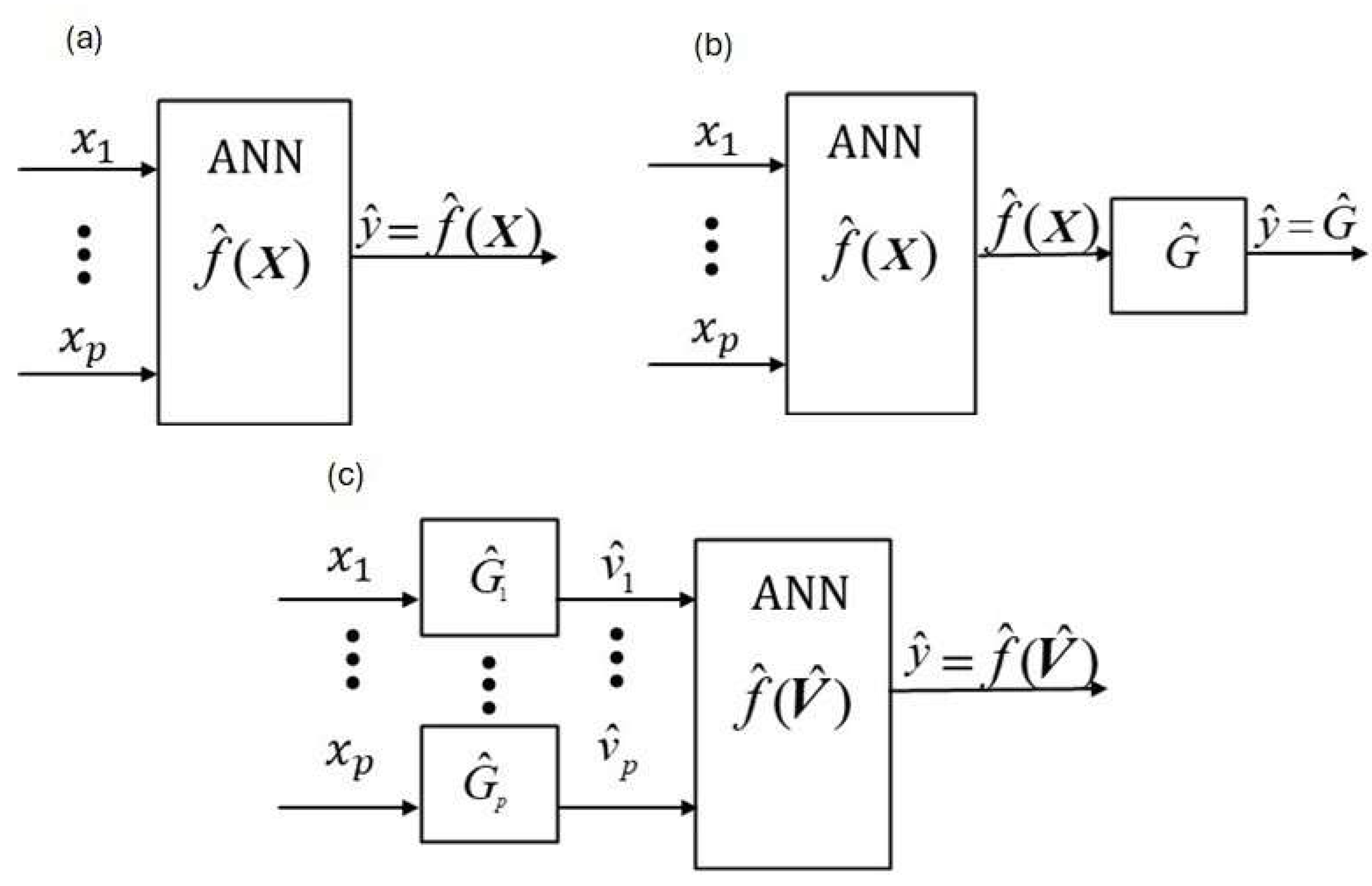
Figure 2.
Python® Stage 2, Model 1, Observed and Fitted, Training and Validation graphical results.
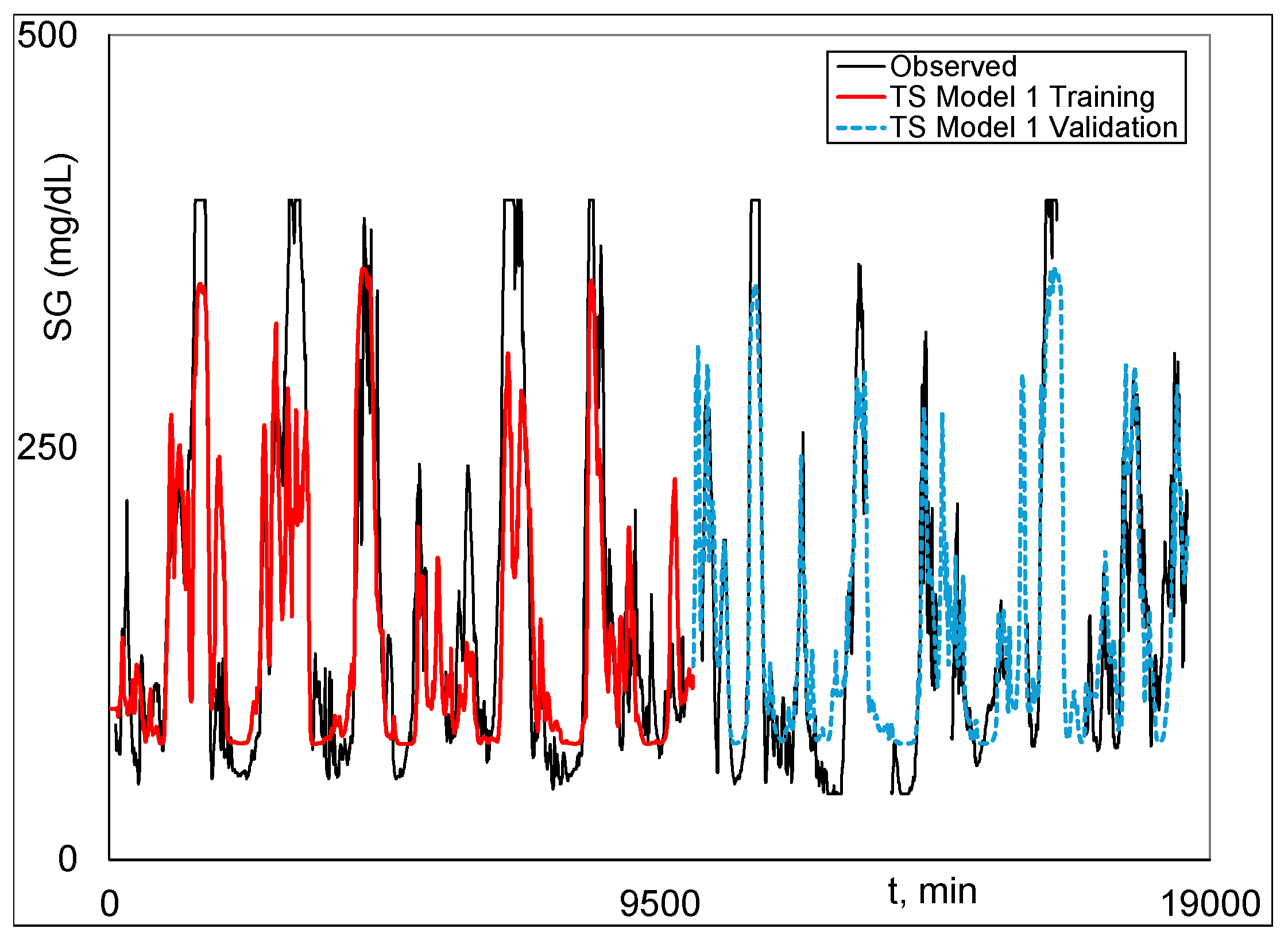
Figure 3.
Python® Stage 2, Model 2, Observed and Fitted, Training and Validation graphical results.
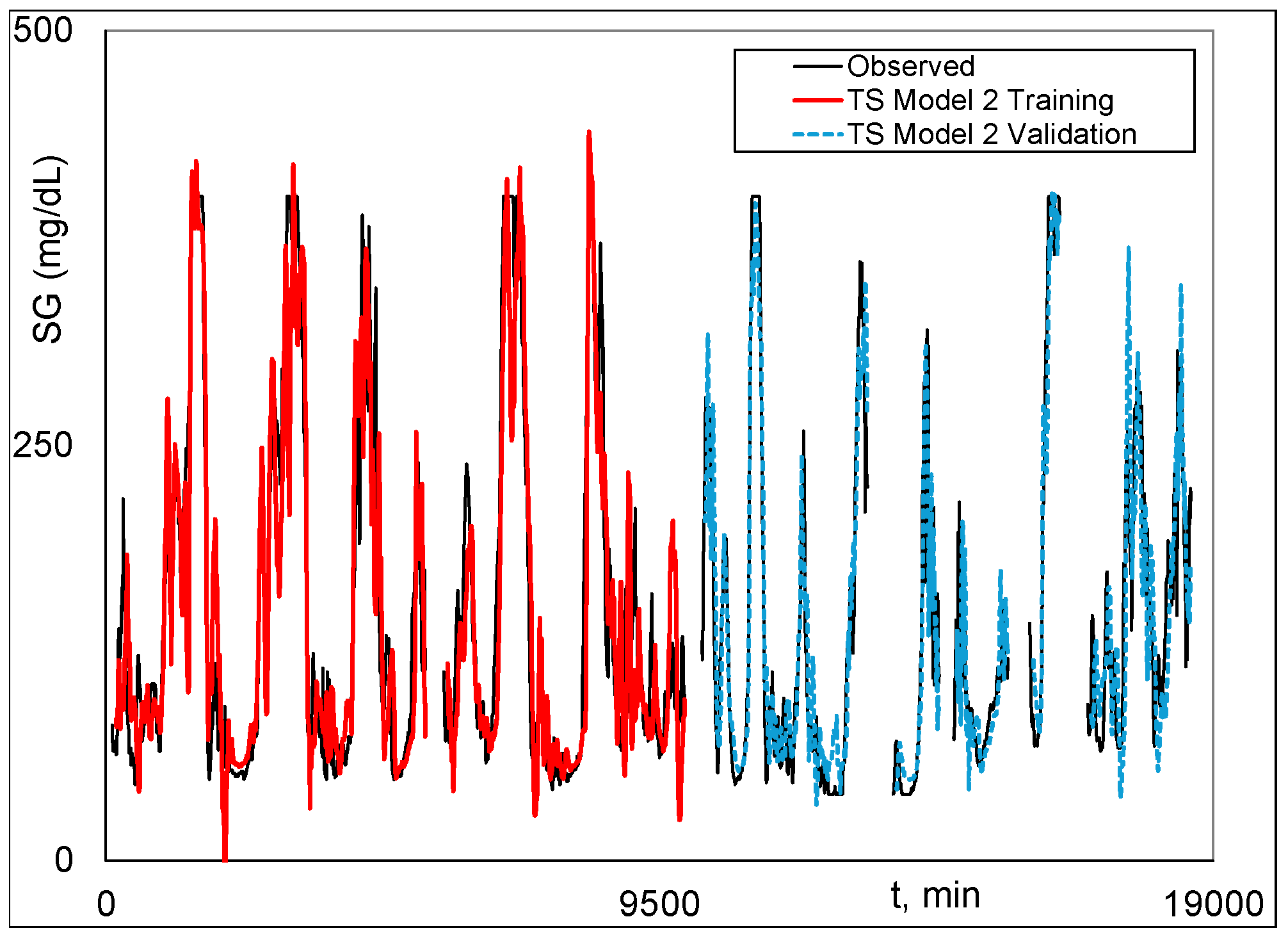
Figure 4.
Python® Stage 2, Model 1-2, Observed and Fitted, Validation graphical results.
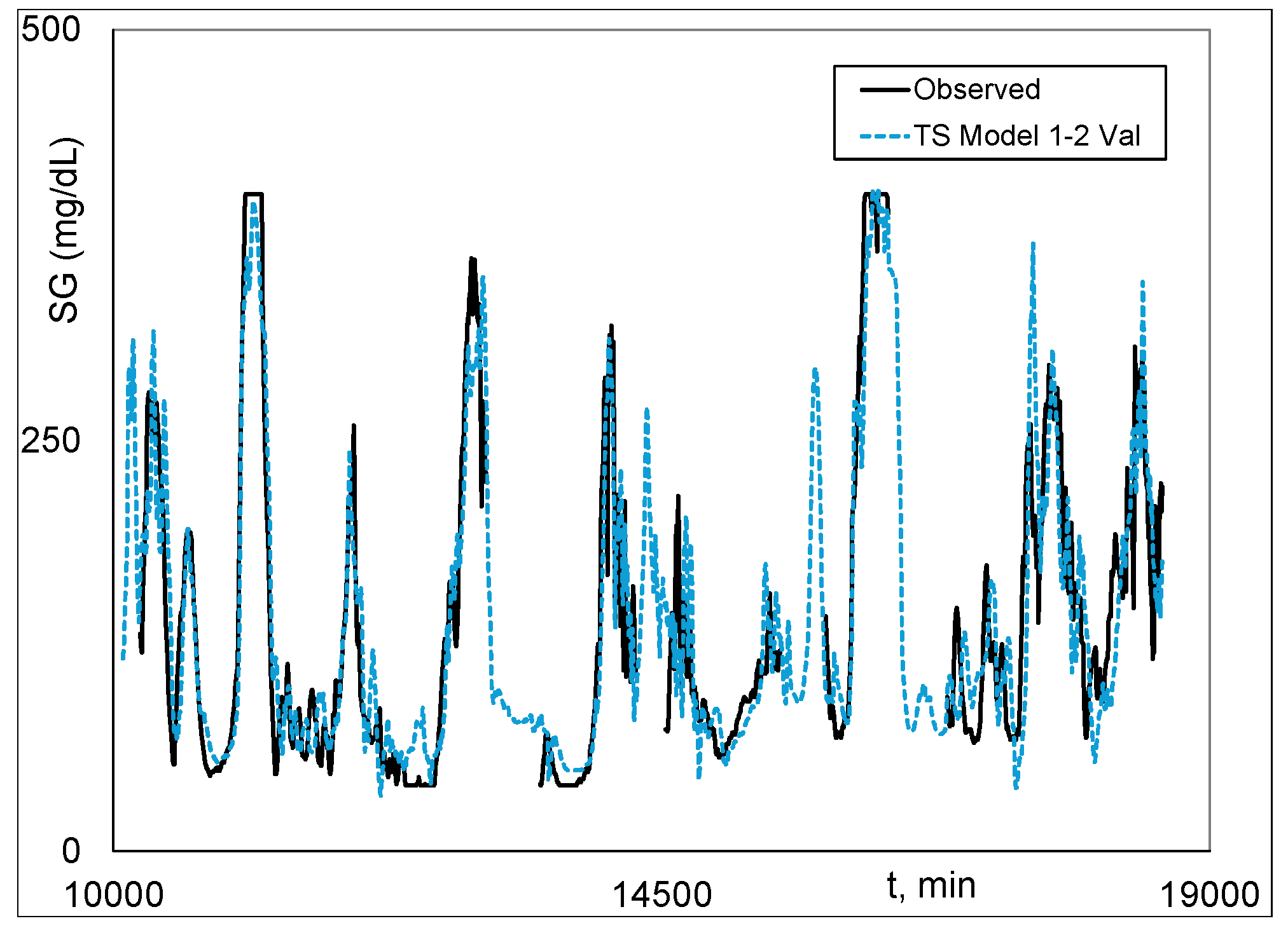

Table 1.
Stages 1 and 2 Modeling Results1.
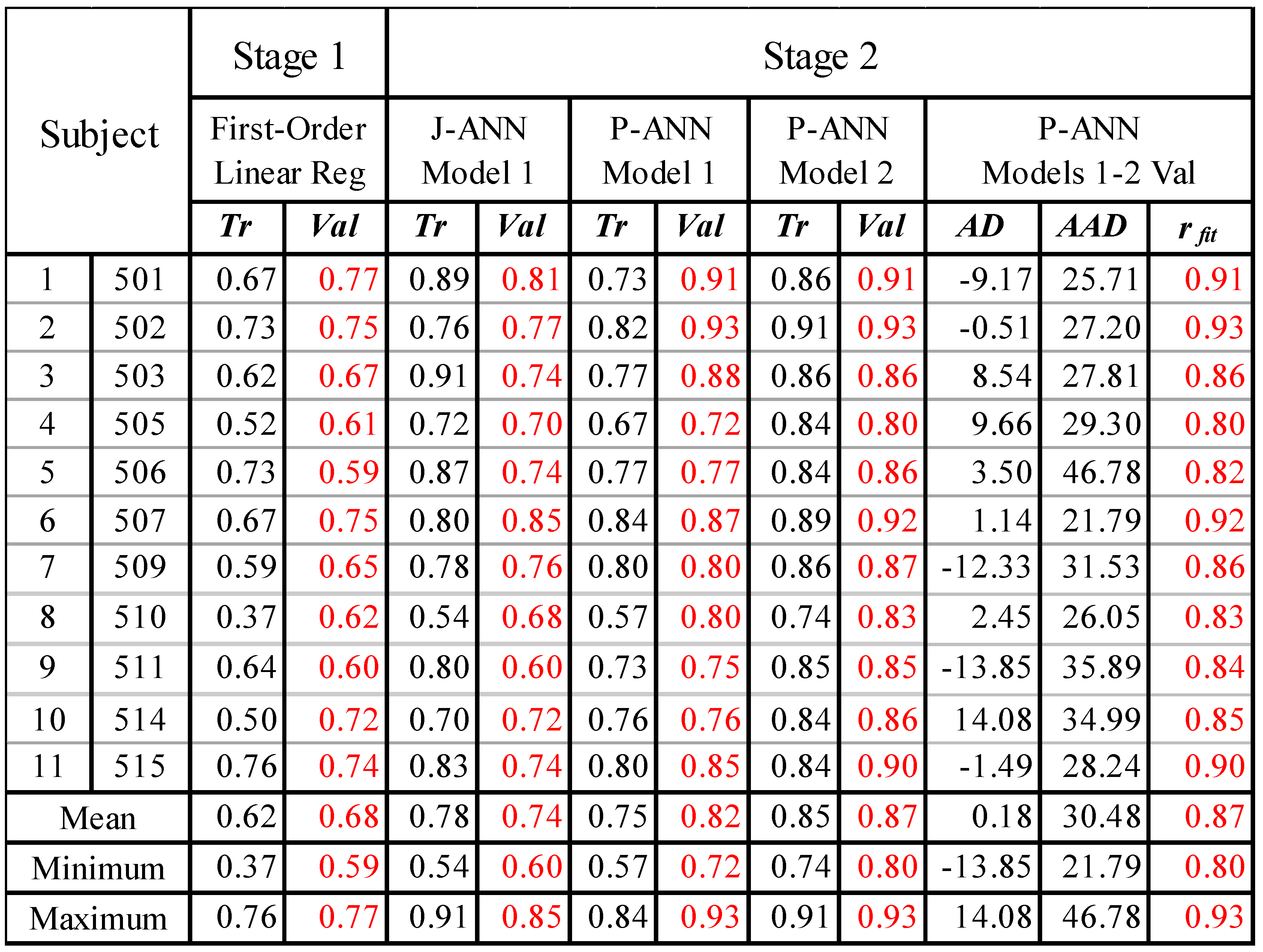
1 All results are rfit unless otherwise indicated. Stage 1 results are for Model 1. J-ANN means JMP® ANN and P-ANN means Python® ANN.
Disclaimer/Publisher’s Note: The statements, opinions and data contained in all publications are solely those of the individual author(s) and contributor(s) and not of MDPI and/or the editor(s). MDPI and/or the editor(s) disclaim responsibility for any injury to people or property resulting from any ideas, methods, instructions or products referred to in the content. |
© 2025 by the authors. Licensee MDPI, Basel, Switzerland. This article is an open access article distributed under the terms and conditions of the Creative Commons Attribution (CC BY) license (http://creativecommons.org/licenses/by/4.0/).
Copyright: This open access article is published under a Creative Commons CC BY 4.0 license, which permit the free download, distribution, and reuse, provided that the author and preprint are cited in any reuse.


