
Submitted:
04 September 2025
Posted:
09 September 2025
You are already at the latest version
Abstract
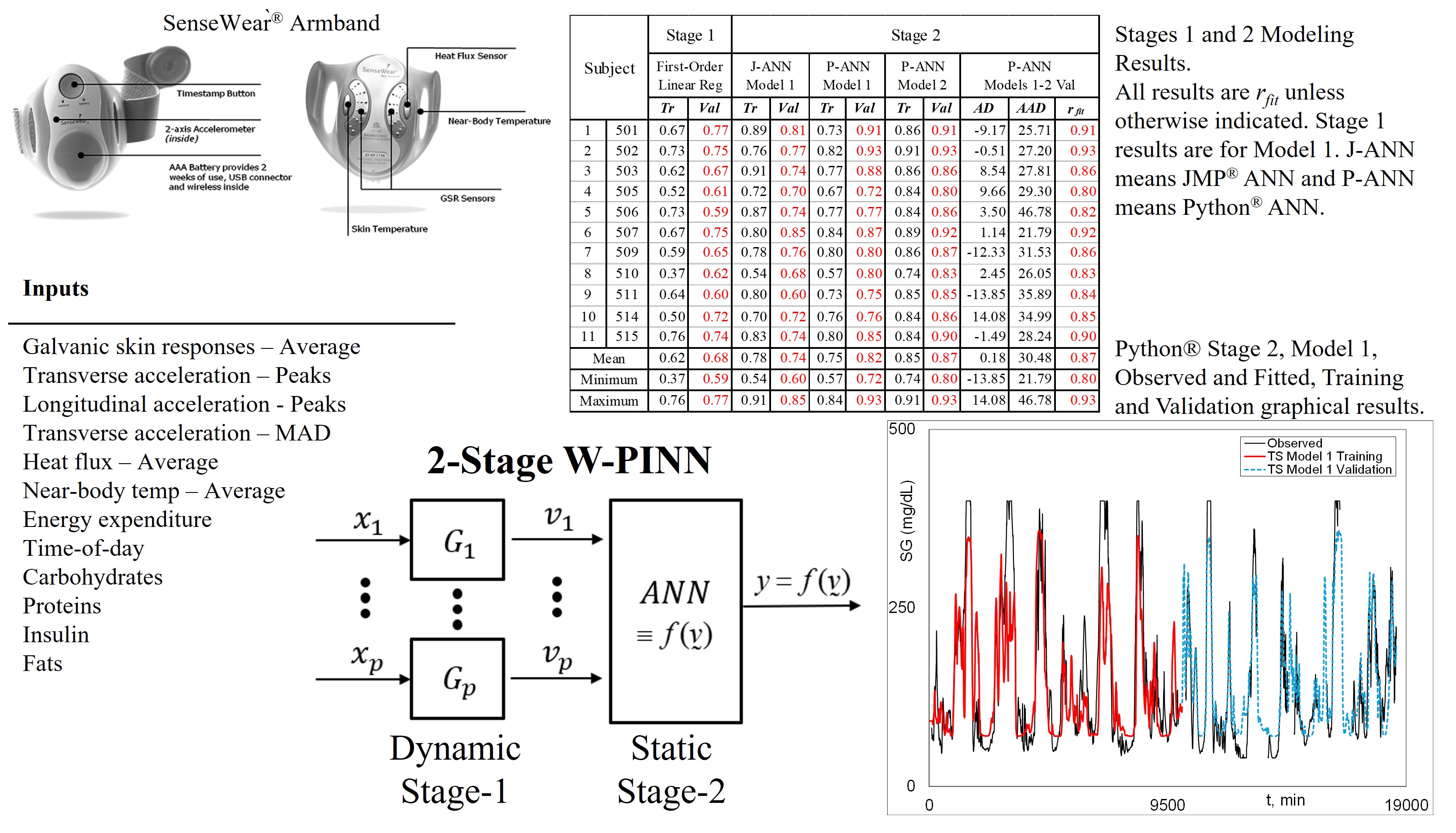
The objective of this work is the development of a sufficiently accurate, cause-and-effect, forecast modeling methodology for closed-loop control of sensor glucose concentration (SGC). The forecast horizon is 60 minutes across eleven cases, representing a critical step toward achieving tight, automatic, 24-hour SGC control. Using free-living data with twelve inputs, this study focuses on a two-stage Wiener Physically-Informed Neural Network (W-PINN) approach to forecast SGC (y). In Stage 1, each static input xi is transformed into its dynamic counterpart vi, forming vector V = (v1, …, vp)T, based on second-order-plus-dead-time-plus-lead dynamic parameters estimated in prior work via first-order linear regression, yielding an average input-only validation fit \( \bar{r} \)fit,val of 0.68. Stage 2, the core of this study, enhances accuracy using artificial neural network (ANN) structures. Two ANN methods were evaluated: one via the JMP® toolbox, achieving an average input-only \( \bar{r} \)fit,val of 0.74 (maximum 0.84), and a custom Python® implementation, attaining 0.82 (maximum 0.93). Incorporating bias correction with current and past SGC residuals in the Python® estimator further improved the 60-minute forecast, with an average rfit,val of 0.87 (maximum 0.93).
Keywords:
block-oriented modeling
; free-living data collection
; glucose modeling
; Hammerstein modeling
; physically informed neural network
; type 1 diabetes
; Weiner modeling
1. Introductionh
Type 1 diabetes (T1D) is a condition that renders the pancreas unable to produce beta cells that are needed to produce insulin to keep blood glucose concentrations (BGC) within a certain range to maintain glycemic homeostasis. High BGC (hyperglycemia) can lead to permanent damage to organs and body functions such as vision, limbs, etc., whereas low BGC (hypoglycemia) can cause seizures, brain damage, loss of consciousness, death, etc. [1,2]. Thus, maintaining healthy BGC is critical and quite challenging for people with type 1 diabetes.
The concept of an artificial pancreas (AP) is a closed-loop glucose control system with the following three main components: 1. a device and/or methodology to infer sensor glucose concentration (SGC), the controlled variable (CV), sufficiently, frequently, and accurately for 24-h online automatic feedback forecast control (AFFC); 2. a suitably precise, effective, and robust manipulated variable (MV) and delivery system (e.g., insulin pump); and 3. an intelligent system for fully 24-h feedback forecast control, diagnosis, and other critical AP tasks. Recently, progress in online knowledge-based (i.e., expert system) algorithms appears to have contributed to modest improvements in classification and aiding in reducing the frequency and magnitude of SGC spikes [3,4,5]. The focus of this work is the first component above. More specifically, the goal of this research is the development of an effective online SGC forecast modeling methodology for effective 24-h AFFC.
The typical behavior of a physical (i.e., nonbiological) automatic control system is that a change in MV will immediately impact its CV. However, when insulin (the MV) is injected into the body, it takes time for it to impact SGC. This time is the true deadtime for this insulin injection (II). The time it takes for SGC to decrease from an II we defined as the true observable deadtime (θMV). One of the major and unique AP control challenges is the existence of θMV. (Bi-hormonal modeling or control is not in the scope of this work. Our assumption is that advancements in SGC forecast modeling can contribute to advancements in bi-hormonal forecast modeling.) Successful (i.e., sufficiently tight) SGC requires accurate II. This objective requires sufficiently accurate cause-and-effect forecast modeling of SGC (the explanatory variable) a θMV distance in the future.
“Forecast” and “Prediction” are often treated as synonyms in casual conversations as well as in the mathematical modeling literature. However, in the context of this work, it is important to distinguish and define them to avoid subtle and critical misunderstandings. Prediction is a word that is commonly used in the statistical literature [6]. However, this use is applied in a static (i.e., nondynamic) context. More specifically, in the statistics literature, a prediction is the value a static (i.e., nondynamic) stochastic variable may become when sampled in the future regardless of how far into the future. This type of modeling (i.e., static) is not in the scope of this work.
In contrast, the value of a forecast (i.e., dynamic) stochastic variable is dependent on the forecast (i.e., time) distance. There are at least two types of forecasting scenarios. The first type, e.g., weather forecasting, seeks to predict future weather conditions but not change them. We call this “forecast monitoring” (FM). AFFC, our objective, seeks to accurately predict the future value of CV, and then effectively and safely manipulate conditions in the present, by changing MV, to drive CV to its target (i.e., set point, SP) after this future distance is reached. Thus, AFFC models SGC (the CV) to determine II (the MV) sufficiently accurately for acceptable SGC automatic control. We strongly believe that this model must be adequately “cause and effect” and developed and evaluated in outpatient studies. Our premise is that an FM methodology that models a correlation structure will fail in an outpatient, free living, AFFC application if it is not sufficiently “cause and effect”. All the SGC models that we have found in this literature model the correlation structure (e.g., see [30,31,32,33]). In contrast, the motivation of our work is to advance AFFC modeling of SGC that we feel will also be helpful in hormone modeling for AFFC for increasing SGC.
There are two ways to develop cause and effect models -- statistical design of experiments (SDOE) and theoretically-based modeling. We classify any experimental design that uses orthogonal (or near orthogonal) input changes for model identification as SDOE. In this context, SDOE does not seem like a practical alternative in general because a significant number of input changes will be highly undesirable and/or impractical (e.g., 100% fat meals). In addition, we feel it is critically important to develop SGC models from free living data to limit subject stress and model under the most comfortable conditions of the subject since studies can run for weeks to get adequate data size to build sufficiently acceptable models.
In AP terms, θMV is the forecast distance, i.e., the amount of future time it takes an insulin injection to start decreasing SGC. However, the forecast,is the predicted value of SGC a θMV distance into the future. Thus, the AP feedback error (FBE) at the current time (t) is et, where et = SGC Setpoint - It is highly critical that et is accurate for all t since it determines the amount of insulin that is injected into the user when the automatic control system is online, i.e., controlling insulin infusion. If the forecast ofis too high, this can lead to hypoglycemia (dangerously low SGC) or if it is too this can lead to hyperglycemia (dangerously high SGC).
Therefore, AP effectiveness is strongly dependent on the estimation accuracy of SGt+θMV, the overall objective of this work. To achieve this objective, this work sets the following conditions (i.e., scope). The first one is that data collection is out-patient (non-hospital) and free-living (determined completely by the subject). Secondly, the training and validation periods are approximately one week each or more. The idea here is that there will likely be some subjects where both data sets include days that have similar and different activities (e.g., working days and non-working days). Thirdly, input data sets must not have missing data. A protocol must be defined and used to estimate missing data such as using the average of the value before the gap and after the gap to fill in the missing data in the gap. This is the method we used to fill in missing input data gaps. No missing input data means no missing forecast (i.e., values. Missing input data results in large gaps in values, and thus, in the ability of the controller to obtain the FBE and, thus, being online. Fourthly, the structure of must be sufficiently parsimonious (low parametrization) and physically interpretable to guard against “curve fitting” to maximize cause and effect behavior, since this is a control application and not a monitoring one. Fifthly, SGC measurements are used to “correct” model bias must be at least a θMV distance in its past (i.e., at t, the current time, or less than t). Lastly, dynamic modeling must be physically-informed. Empirical modeling has a strong tendency to fit to correlation structures in data. Free-living data inherently has correlation structures, as humans are creatures of habit. Experimentally designed data sets with orthogonal input changes can produce cause-and-effect, empirical models. However, in this application, experimentally designed data is not realistic as mentioned above. Physically-informed modeling can provide cause-and-effect modeling from free-living data when the variables with physical interpretation are estimated accurately, and physical constraints are met. More specifically, now, the objective of this work is the development of a sufficiently accurate control application SGt+θMV approach meeting these six criteria.
As mentioned above, in-patient (hospital clinical) or simulation studies are not in the scope of this work. However, they can provide valuable insights into the development of outpatient studies. In-patient and simulation studies commonly have durations of a few hours to a couple of days (see [7,8,9,10,11,12,13,14,15,16,17,18,19,20,21,22,23,24,25,26,27,28,29,30,31,32,33]).
There are several interesting outpatient modeling studies in the literature as well. For example, see [34,35,36,37,38,39,40,41,42,43,44]. However, we have not found any study in this literature meeting all six of our criteria. While there are a few studies meeting several of these criteria, no methodology, but our proposed approach, meets the sixth one, “dynamic modeling must be physically-informed.” All the ones that we have found are empirical modeling approaches.
We strongly advocate for the following three performance statistics for quantitative comparative methodological evaluation (the formulas for each will be given later). The measure of performance that is the least found in this literature is rfit. This statistic quantifies how well the fitted model increases and decreases with SGC data, with an upper limit of rfit = 1. Results that only show fit visually are considerably less informative than ones that give both the visual results and the quantitative results, which makes it possible to compare methods quantitatively and to set a numerical goal. For example, our rfit validation goal is 0.9. We have found only a few studies in this literature reporting rfit results [45,46,47].
The second type of statistic that we use measures spread, i.e., variability of the difference between the measured and fitted values. Statistics are typically given for at least one measure of spread in the SGC modeling literature. A popular one has been called the root mean squared error (RMSE) [48,49]. This statistic is a measure of spread, and more specifically, the standard deviation of the difference between measured SGC and fitted SGC. The drawbacks of this statistic include not being easily interpretable quantitatively since it is distributionally dependent, which can vary considerably across studies and the methodology used. Thus, similar values, quantitatively, can be very different inferentially based on the true probability distribution of the statistic. Notwithstanding, the measure of spread that we prefer to use is the average of the absolute differences (AAD) of measured and fitted values. AAD is easily interpretable across studies since it is an average of the magnitude of the differences, i.e., a measure of its centrality of absolute deviation. For example, for a data set with differences from its mean value of -30, 30, 30, -30, AAD is 30; in other words, the average distance from its mean value of zero is 30.
The final statistic that we advocate to be used is a measurement of model bias and is the average difference (AD) of measured and fitted SGC values. We have not seen this statistic reported much in the SGC modeling literature. However, its reporting is crucial to an overall assessment of a methodology. For example, if rfit = 0.99 and AD is large positively or negatively, the model was excellent in following the increasing and decreasing behavior of the observed SGC but is quite biased. For the AAD example above, AD = 0. However, for the data set of -30, -30, -30, -30, AAD is still 30, but AD is -30, and, therefore, has a higher estimated modeling bias.
Thus, for each subject, our validation modeling goal is high rfit,val (rfit for validation), low AAD, and low AD. In practice, these values will be subject-specific. However, until we test our methodology in closed-loop studies, we have set a quantitative modeling goal for fit only. It is rfit,val 0.90, which is quite ambitious for large, highly complex, outpatient, free-living SGC datasets.
As mentioned above, methodologies should not model an input with a modeled dead time less than θMV unless its value is known at t + θi where θi < θMV, e.g., for meal-announced carbohydrates. This is because a real time dynamic θMV forecast prediction model for a control application can only use current, or earlier than current, input data (excluding announcement inputs) as mentioned above.
Classical ANN in this context is a one-block, completely empirical modeling approach as illustrated in Figure 1a. All the inputs enter this block, and a mathematical structure with adjustable parameters (i.e., coefficients or “weights) is changed to obtain an acceptable agreement with measured response data. When the functions use lagged variables, it is an empirical dynamic model structure.
The work by Pun et al. is some of the earliest work on “Physically-Informed-Neural-Network (PINN)” that was found [50]. However, the work in [51] presented PINN with a two-block structure shown in Figure 2, aligning more clearly with the model representations in this work. As shown, the inputs enter a static ANN block (i.e., one with no lag variables), and its output variable enters a theoretically (i.e., physically) based block (i.e., model structure). We recognized Figure 2 as a Hammerstein Block-Oriented Structure [52] when its second block is a physically informed (i.e., interpretable) linear dynamic structure (G), that we have named H-PINN (as shown in Figure 1b). When physically interpretable linear dynamic blocks (Gi) are followed by a static ANN block, as in Figure 1c, this is a Wiener Block-Oriented Structure, which we have given the name W-PINN.
The aims of this study are to develop and evaluate two, 2-stage W-PINN methodologies, using the vi’s of eleven (11) Type 1 diabetes models in a manuscript currently in review and posted at https://drollins9.wixsite.com/derrickrollins. Our arbitrary, but ambitious, goal is to achieve an rfit,val 0.90 on at least one of the data sets using input data only (defined as Model 1). The first methodology estimates f(V) (see Figure 1c) using the ANN package in JMP®. The second methodology estimates f(V) using a Python® coded methodology that we developed.
2. Materials and Methods
The eleven free-living, Type 1, glucose data sets used in this work uses were first modeled in [53] and later by [54]. However, neither dynamically modeled these data sets for a closed-loop control application since θMV equaled zero in both. Thus, these studies are not applicable to AFFC, the application for this work.
[53] generated these data sets in 2011. Their SGC sampling rate, Δt, is 5 min, and all twelve (12) inputs have this sampling rate as required for discrete-time modeling. The inputs include lifestyle, activity, food consumption, stress, physiological changes, and time of day (i.e., the 24-h clock). When these data sets were obtained, the Medtronic glucose sensor required replacement every three to four days and had a much longer warm-up period than current devices. Due to variations in SGC missing data, the data set sample size (n) varied from 3,733 to 4,837. Subject-reported food logs for carbohydrates, fats, and proteins were used. We note that while the activity tracker was innovative for this study at the time, it did not have the most critical sensor, heart rate, and its technology is considerably less advanced than today’s wearable activity devices and, thus, obsolete by today’s standards. We combined bolus and basal insulin and reduced the number of inputs by one, to twelve. These data sets are available to the public on the website of the first author at https://drollins9.wixsite.com/derrickrollins. For additional details of the inputs and the data collection, see [53].
2.1. W-PINN
Our W-PINN approach uses backward difference derivatives (BDD) to discretize second-order-plus-dead-time-plus-lead (SOPDTPL) (see [55]) theoretical dynamic systems, the only type used in this work, as given in Eq. 1, below. The dynamic system does not have to be initially at a steady state for our W-PINN modeling methodology since this initial condition is also estimated. Note that, Eq. 1, below, is the expression for each of the p-inputs.
with
where andfor i = 1, …, p, xi(t) is the value of the ith input variable at t, and vi(t) is the value of the ith output variable at t, in the units of xi, y(t) is the output variable in its units at t, means the expected value (i.e., true mean) of y(t),is the true output (gain) function of V(t), the vector of the vi(t)’s. Whenis a nonlinear function of V(t), as in the ANN (i.e., W-PINN) case, Eqs. 1 and 2, taken together, have a Wiener block-oriented structure [47], as shown in Figure 1c.
The lead term is the first term on the right side of the equal sign in Eq.1. This term tends to “speed up” the response and provides what the process modeling and control community has termed “numerator dynamics” [51,52]. [47] developed a second-order, multiple-input, single-output, discrete-time, nonlinear Wiener dynamic approach using BDD based on Eq. 1. More specifically, using BDD approximation applied to a sampling interval of Δt, an approximate discrete-time form of Eq. 1 is
with
such that to satisfy the unity gain constraint. From Eq. 3 with
After obtainingfor each input i, the modeled output value, at time t, is determined by entering these results into, a static ANN in this application, i.e.,
2.2. Stage 1 Modeling Method
As mentioned above, Stage 1 of this two-stage methodology is completed. This work is in review and posted at https://drollins9.wixsite.com/derrickrollins. We now give important Stage 1 details and results to aid in the understanding of the Stage 2 methodology. While missing output (i.e., SGC) measurements are acceptable, missing input values are not for discrete-time modeling. Activity tracker data were the only missing input data. These missing values were estimated by averaging the two values on both sides of a gap and filling in the gap with this value. Some gaps were several hours long. Cross-validation [57] was used to guard against overfitting, with the first week as the training (Tr) data set, and the second week as the validation (Val) data set.
In Stage 1, all inputs were first modeled separately on their own Excel® worksheet with a first-order linear regression function. For each case, insulin was modeled first. The estimated deadtime, i.e., was set at 60 min and was varied one Dt forwards and backwards to find the value that gave the best fit. For all the inputs, the estimate of θMV, , was determined to be 60 min, i.e., 12 Dt. The food variables were the only ones with announcements, and the carbohydrate input was the only one found to have a deadtime less than . The “time of day” input has no deadtime, and the dead time for all other inputs was, except for fats that had deadtimes that were much larger than, as determined by model estimation. After determining the dynamic estimates for each input (i.e., Eqs. 4 to 6), these values were copied to an Excel® worksheet as the dynamic structure starting values for fitting the SOPDTPL dynamic, and first-order static, multiple-input model (i.e., Eq. 10). With f(V) as a first-order multiple linear regression static function, the fixed estimate of V, , for Stage 2 was determined.
2.3. Stage 2 Model Development Modeling Methods
The objective of this work is the development, evaluation, and comparison of two, Stage 2, W-PINN modeling approaches using from Stage 1 to obtainfor each of the eleven cases for the two approaches. The first approach uses the JMP® ANN toolbox to approximately find the smallest SSE (i.e., SSR) by fitting many cases and selecting the best one. The second approach is a newly developed, confidential, ANN structure that is coded using Python®. Both approaches significantly improved fit over the first-order regression function. A diagram illustrating the general ANN Stage 2 approach for obtaining is given in Figure 1c.
2.4. Three Input Models
There are three types of input model structures we have developed for this application. The first one we call the “input only model” or “Model 1.” All the inputs in this structure have a deadtimeexcept for announcement inputs that can have deadtimes less thanlike carbohydrates, equal tolike proteins, greater thanlike fats, and zero like time of day.
The second one we call the “input-output model” or “Model 2.” It combines the input-only structure of Model 1 (i.e., Eq. 10) with a model of weighted residuals, a minimum of distance in the past, as shown in Eq. 11 below (see [45] for the derivation).
where Eq. 11 has no value if any residual is not determinable due to missing output measurements. Thus, unlike Model 1, which has estimates for all t since it uses only input data, Model 2 will not have estimates when outputs are missing.
The final model, Model 1-2, is a combination of the strengths of Models 1 and 2. More specifically, for Model 1-2,
2.5. Forecast Structures
Equation 10,, is the model development version of Model 1 as it is used to estimate the output, y, at the current time, t. There are no missing input values in Eq. 10. This is why missing armband data had to be estimated. In addition, non-announcement input values to obtain Eq. 10 must be at least a distance of in the past. This requirement is because the model development input lag must be the same as the forecast input lag, i.e., at t, for forecasting adistance into the future.
After obtaining , its transformation into the kΔt forecast, i.e., the online version, is given by Eq. 13 below:
where, from Eq. 7, with t = t + kΔt,
Note that, if k = 12 and Δt = 5 min, the Eq. 14 model is forecasting 60 min into the future. Thus, all the non-announcement inputs must have a model building and forecast prediction dead time of at least 60 min.
2.6. Statistical Analyses
The first, and most important, modeling statistic is rfit (which is bounded between -1 and 1), the fitted correlation of the measured SGC,, and the fitted SGC,, and given in Eq. 15 below.
where n is the number of samples in the set and the bar above a statistic means that it is its sample mean value. The equations to determine AAD and AD are, respectively,
The equation for SSE (i.e., SSR, the sum of squared residuals), the more common name and used by JMP®, is
3. Results
Training and Validation Stage 1 and Stage 2 summary statistics for the eleven subjects are given in Table 1. All the results are rfit unless indicated otherwise. Recalling that, each subject has a fixedthat was determined in Stage 1 using the first-order static structure as given in Eq. 19, below:
As shown, Stage 1, Model 1, rfit,val results varied from 0.59 to 0.77, with a mean of 0.68. Moreover, Stage 2 Model 1 rfit,val results improved significantly over the Stage 1 results for both ANN approaches. As shown, JMP® Stage 2 Model 1 rfit,val results varied from 0.60 to 0.85, with a mean of 0.74. However, Python® Stage 2 Model 1 rfit,val results are significantly better than JMP®, varying from 0.72 to 0.93, with a mean of 0.82. As a result, Model 2 training and validation results, and Models 1-2 validation results are given in Table 1 for Python® only. From Model 1 to Model 2, the Python® mean rfit,val increased from 0.82 to 0.87, the minimum from 0.72 to 0.80, and the maximum of 0.93 did not change. In summary, Python® Stage 2 results improved considerably over Stage 1 results and are significantly better than JMP® Stage 2 results.
Graphical Python® Stage 2 fitted and measured SGC results for Subject 2 (the best case) are given (i.e., plotted) in Figure 3, Figure 4 and Figure 5. Figure 3 is Model 1 training and validation. Figure 4 is Model 2 training and validation. Figure 5 plots are the combined validation results, with Model 1 plotted when there is no output data, and Model 2 is plotted when there is output data, i.e., the Model 1-2 validation plot. The Model 1-2 plots are associated with the results in the last three columns in Table 1. Figure 4 shows an excellent fit of Model 2 and the highly realistic behavior of Model 1 when Model 2 results are not possible because of missing SGC data (see Eq. 11).
4. Discussion
In this study, two physically-based virtual forecasting sensor approaches were developed for obtaining the value of the controlled variable (CV), SGC, a θMV time distance in the future, for a two-stage closed-loop process control application. The first stage, a physically (i.e., theoretical) based dynamic modeling approach [47] estimates the physically interpretable dynamic parameters from the measured inputs (xi’s) with multiple physical constraints to obtain dynamic outputs (vi’s). The vi’s are the inputs to the second stage, a static ANN structure. For the first method, this structure was determined by using the ANN toolbox in JMP®. For the second method, this structure was determined by using a confidential method that this work developed and coded using Python®. Both methods resulted in large average improvements over the Stage 1 results using a first-order linear regression static structure (see Table 1). In addition, a critical advantage of these two approaches is that the modeling is much easier and much less time-consuming than the 2nd order multiple linear regression (MLR) approach. Thus, we strongly recommend ANN over MLR for the static model structure. Note that ANN modeling is just a particular class of multiple nonlinear regression. The MLR model was applied to Subject 11 to compare the performance with the ANN. The rfit,val had a modest improvement from Stage 1 alone, going from 0.74 to 0.79, but much less than the 0.85 obtained for P-ANN.
We were pleasantly surprised by the P-ANN achievements of Models 1, 2, and 1-2. Model 1 has two subjects over the rfit,val goal of 0.90 and a mean of 0.82. Model 2 has four subjects meeting or exceeding the rfit,val goal and a significant increase in the mean rfit,val of 0.87. The combined Model 1 and Model 2 approach, i.e., Models 1-2, had essentially the same summary statistics results as Model 2, as shown in Table 1. Thus, combining Models 1 and 2, to have continuous forecasting without missing fits did not adversely affect rfit,val relative to Model 2, which had missing fits due to missing SGC measurements.
Insulin is the process variable that is changed to keep SGC close to its set point, i.e., it is the manipulated variable (MV). For the control system to do this well in a forecast feedback control scheme, the controlled variable, SGt+θMV, must be accurately estimated. An empirical method could possibly control SGt+θMV online accurately if the correlation structure remains the same as it was when the model was developed. However, it is not possible for the correlation structure of an empirical forecast modeling approach in this context to remain intact, i.e., fixed, in online forecast feedback control because the correlation structure changes each time the controller signal to the manipulated variable is transmitted. Thus, it is prudent to restrict free-living empirical modeling to monitoring open-loop processes but not to make decisions on how much to change a manipulated variable to make changes in the control variable.
During his time as a professor, the second author gained valuable insight into the limitations of empirical modeling through a real-world industrial application. A BS Chemical Engineering student, also pursuing an MS in Statistics, undertook a summer project at a leading Midwest chemical company, which was approved as the basis for her MS thesis. The project focused on developing a multivariate Statistical Process Control (SPC) monitoring methodology for a process line. Data were collected, and an SPC control chart was developed, resulting in an excellent model fit. However, when the process exceeded control limits, adjustments to the manipulated variable based on this model failed to restore control. A subsequent attempt with new data and a revised control chart, despite another excellent fit, similarly failed to correct deviations when applied in a feedback control scenario. This experience highlighted that the control chart, designed for monitoring, was unsuitable for feedback control due to its reliance on empirical correlation rather than cause-and-effect relationships. Empirical SGC modeling, which uses free-living data and non-physiological structures, faces similar limitations, as it cannot adequately capture cause-and-effect dynamics critical for model-based control applications like automatic forecast control. In contrast, physically-informed modeling, which integrates physiological information and structure with free-living data, offers inherent intelligence and robust structure for developing effective models for control applications. The W-PINN methodology proposed in this manuscript exemplifies such an approach, enabling cause-and-effect modeling suitable for closed-loop SGC control.
A limitation of the proposed two-stage W-PINN approach is the sequential estimation of parameters, with dynamic modeling parameters determined in Stage 1 and static modeling parameters in Stage 2. A more robust, yet considerably more complex, alternative is a one-stage approach that estimates all parameters simultaneously. Our research group is currently developing this method, with implementation in Python, aiming to complete the work and draft a manuscript within approximately one month. We anticipate that this one-stage approach will yield significant but moderate improvements in model performance compared to the two-stage W-PINN methodology.
A drawback of the proposed two-stage W-PINN approach is that the dynamic modeling parameters are estimated in Stage 1 and the static modeling parameters are estimated in Stage 2. A better but significantly more challenging approach is to estimate all modeling parameters in a One Stage approach. Our research group is working on this development and hopes to complete this work and write this manuscript in a month or so. It will be coded using Python and our expectation is a significant but modest improvement over our Two-Stage approach.
Two very popular empirical dynamic modeling approaches are Nonlinear Autoregressive Moving Average with eXogenous variables (NARMAX) [43,58,59] and Long and Short Term Memory (LSTM) [60]. Our research group evaluated NARMAX in [61] using real, freely-existing distillation column data. The ten (10) data sets, covering a period of three years, were generated by undergraduate chemical engineering students for their unit operation lab course. For this data set, [54] was not able to find adequate starting values to obtain a NARMAX lagged-based fit using Matlab®. They transformed NARMAX into a physically-informed (N-PINN) structure and compared the results of the eight (8) test cases. The mean testing rfit (i.e., rfit,ts) for W-PINN and N-PINN, were 0.84 and 0.28, respectively. We plan to evaluate LSTM against our one-stage W-PINN approach using the diabetes data sets in this work and these distillation column data sets.
5. Conclusions
Type 1 diabetes SGC modeling for monitoring can be effective (i.e., informative) using empirical or physically-informed dynamic modeling approaches. Closed-loop Type 1 SGC automatic control is inherently forecast automatic control because a change in MV, injected insulin, will take a time of θMV to start lowering SGC. For automatic closed-loop control, empirical dynamic modeling approaches are not likely to succeed because they lack a cause-and-effect relationship, unlike Physical Informed Neural Network (PINN) approaches. The W-PINN approach, developed in this work, is particularly powerful because each input xi is dynamically transformed to its vi and is the input to a static ANN. The proposed two-stage W-PINN approach greatly improved the SGC model fit for eleven historical diabetes data sets. A one-stage W-PINN approach, in its evaluation stage, is the next step in this research.
There are several drawbacks to the data sets used in this work. First, they are nearly a decade and a half old, particularly in terms of the amount of missing or lost data. Glucose sensor technology and activity tracker technology have improved considerably and particularly in terms of the amount of missing or lost data, also. In addition, there are advancements in ways to get accurate consumption of food nutrients. Thus, one future goal is to evaluate the methodology using modern technology.
Since this is a forecast control application modeling free-living data, to get a more informative evaluation of a methodology, we feel it is critical to collect a minimum of 3 weeks of free-living outpatient data (one week each for training, validation, and testing). However, we feel that four would be more ideal with two weeks of testing data.
The most important input is SGC. We feel that it is an open question as to whether it is the only needed input because it is the MV. Since several inputs, like the three (3) nutrients, have a big influence on the level of SGC but no role as contributors to the MV, we may discover that the number of critical inputs for effective automatic feedback forecast control (AFFC) is a very short list and fit performance will be relative to the maximum possible abilities of the critical inputs.
Supplementary Materials
The data sets are available to the public on the website of the corresponding author at https://drollins9.wixsite.com/derrickrollins.
Author Contributions
For research articles with several authors, a short paragraph specifying their individual contributions must be provided. The following statements should be used “Conceptualization, D.R. and D.H.; methodology, D.R. and D.H.; software, D.H. and Y.G.; validation, D.H., Y.G. and D.R.; formal analysis, D.R., and D.H.; investigation, D.H.; resources, D.R., M.L. and D.H.; data curation, D.H. and J.O.; writing—original draft preparation, D.H.; writing—review and editing, D.R. Y.G. and J.O.; visualization, D.H.; supervision, D.R.; project administration, D.R.; funding acquisition, M.L. All authors have read and agreed to the published version of the manuscript.
Funding
Not applicable as the work is part of the PhD research of Dillon G. Hurd with Dr. Rollins as Major Professor and Dr. Lamm as Co-Major Professor. Jacob Oyler was supported by the National Science Foundation under Grant No. EEC 1852125.
Institutional Review Board Statement
Not Applicable.
Informed Consent Statement
Not Applicable.
Data Availability Statement
The data sets are available to the public on the website of the corresponding author at https://drollins9.wixsite.com/derrickrollins.
Conflicts of Interest
The authors declare no conflicts of interest.
References
- Cryer, P.E. Hypoglycemia, Functional Brain Failure, and Brain Death. J Clin Invest 2007, 117, 868–870. [Google Scholar] [CrossRef]
- Reno, C.M.; Skinner, A.; Bayles, J.; Chen, Y.S.; Daphna-Iken, D.; Fisher, S.J. Severe Hypoglycemia-Induced Sudden Death Is Mediated by Both Cardiac Arrhythmias and Seizures. Am J Physiol Endocrinol Metab 2018, 315, E240–E249. [Google Scholar] [CrossRef] [PubMed]
- Guemes, A.; Cappon, G.; Hernandez, B.; Reddy, M.; Oliver, N.; Georgiou, P.; Herrero, P. Predicting Quality of Overnight Glycaemic Control in Type 1 Diabetes Using Binary Classifiers. IEEE J Biomed Health Inform 2020, 24, 1439–1446. [Google Scholar] [CrossRef]
- Sun, Y.; Kosmas, P. Integrating Bayesian Approaches and Expert Knowledge for Forecasting Continuous Glucose Monitoring Values in Type 2 Diabetes Mellitus. IEEE Journal of Biomedical and Health Informatics 2025, 29, 1419–1432. [Google Scholar] [CrossRef]
- Chico, A.; Moreno-Fernández, J.; Fernández-García, D.; Solá, E. The Hybrid Closed-Loop System Tandem t:Slim X2TM with Control-IQ Technology: Expert Recommendations for Better Management and Optimization. Diabetes Ther 2024, 15, 281–295. [Google Scholar] [CrossRef]
- Devore, J. Probability and Statistics for Engineering and the Sciences, 9th edition; Cengage Learning: Boston, MA, 2015; ISBN 978-1-305-25180-9. [Google Scholar]
- Cichosz, S.L.; Frystyk, J.; Hejlesen, O.K.; Tarnow, L.; Fleischer, J. A Novel Algorithm for Prediction and Detection of Hypoglycemia Based on Continuous Glucose Monitoring and Heart Rate Variability in Patients With Type 1 Diabetes. J Diabetes Sci Technol 2014, 8, 731–737. [Google Scholar] [CrossRef]
- Kamalraj, R.; Neelakandan, S.; Ranjith Kumar, M.; Chandra Shekhar Rao, V.; Anand, R.; Singh, H. Interpretable Filter Based Convolutional Neural Network (IF-CNN) for Glucose Prediction and Classification Using PD-SS Algorithm. Measurement 2021, 183, 109804. [Google Scholar] [CrossRef]
- Eren-Oruklu, M.; Cinar, A.; Quinn, L. Hypoglycemia Prediction with Subject-Specific Recursive Time-Series Models. J Diabetes Sci Technol 2010, 4, 25–33. [Google Scholar] [CrossRef]
- Eren-Oruklu, M.; Cinar, A.; Quinn, L.; Smith, D. Estimation of Future Glucose Concentrations with Subject-Specific Recursive Linear Models. Diabetes Technology & Therapeutics 2009, 11, 243–254. [Google Scholar] [CrossRef] [PubMed]
- Turksoy, K.; Bayrak, E.S.; Quinn, L.; Littlejohn, E.; Cinar, A. Guaranteed Stability of Recursive Multi-Input-Single-Output Time Series Models. In Proceedings of the 2013 American Control Conference; June 2013; pp. 77–82. [Google Scholar]
- Bequette, B.W. Continuous Glucose Monitoring: Real-Time Algorithms for Calibration, Filtering, and Alarms. J Diabetes Sci Technol 2010, 4, 404–418. [Google Scholar] [CrossRef]
- Zarkogianni, K.; Mitsis, K.; Arredondo, M.-T.; Fico, G.; Fioravanti, A.; Nikita, K.S. Neuro-Fuzzy Based Glucose Prediction Model for Patients with Type 1 Diabetes Mellitus. In Proceedings of the IEEE-EMBS International Conference on Biomedical and Health Informatics (BHI); June 2014; pp. 252–255. [Google Scholar]
- Zaidi, S.M.A.; Chandola, V.; Ibrahim, M.; Romanski, B.; Mastrandrea, L.D.; Singh, T. Multi-Step Ahead Predictive Model for Blood Glucose Concentrations of Type-1 Diabetic Patients. Sci Rep 2021, 11, 24332. [Google Scholar] [CrossRef]
- Turksoy, K.; Quinn, L.T.; Littlejohn, E.; Cinar, A. Artificial Pancreas Systems: An Integrated Multivariable Adaptive Approach. IFAC Proceedings Volumes 2014, 47, 249–254. [Google Scholar] [CrossRef]
- Eren-Oruklu, M.; Cinar, A.; Colmekci, C.; Camurdan, M.C. Self-Tuning Controller for Regulation of Glucose Levels in Patients with Type 1 Diabetes. In Proceedings of the 2008 American Control Conference; June 2008; pp. 819–824. [Google Scholar]
- Cameron, F.; Wilson, D.M.; Buckingham, B.A.; Arzumanyan, H.; Clinton, P.; Chase, H.P.; Lum, J.; Maahs, D.M.; Calhoun, P.M.; Bequette, B.W. Inpatient Studies of a Kalman-Filter-Based Predictive Pump Shutoff Algorithm. J Diabetes Sci Technol 2012, 6, 1142–1147. [Google Scholar] [CrossRef] [PubMed]
- Shanthi, S.; Kumar, D.; Varatharaj, S.; Santhana, S. Prediction of Hypo/Hyperglycemia through System Identification, Modeling and Regularization of Ill-Posed Data. International Journal of Computer Science & Emerging Technologies.
- Eren-Oruklu, M.; Cinar, A.; Quinn, L.; Smith, D. Blood Glucose Regulation with An Adaptive Model-Based Control Algorithm. In Proceedings of the ResearchGate; November 2008.
- Professors, Department of ECE, Saveetha School of Engineering, SIMATS, Chennai, Tamilnadu, India; Shanthi*, Dr.S.; Bharath, Dr.S.; Professors, Department of ECE, Saveetha School of Engineering, SIMATS, Chennai, Tamilnadu, India; Sujatha, Dr.M.; Professors, Department of ECE, Saveetha School of Engineering, SIMATS, Chennai, Tamilnadu, India Data Based Estimation of Near Future Values of Blood Glucose with K-Nearest Neighborhood Algorithm. IJITEE 2019, 8, 1438–1442. [CrossRef]
- Kafali, O.; Schaechtle, U.; Stathis, K. Hydra: A Hybrid Diagnosis and Monitoring Architecture for Diabetes. In Proceedings of the 2014 IEEE 16th International Conference on e-Health Networking, Applications and Services (Healthcom); IEEE: Natal, October, 2014; pp. 531–536. [Google Scholar]
- Hughes, C.S.; Patek, S.D.; Breton, M.D.; Kovatchev, B.P. Hypoglycemia Prevention via Pump Attenuation and Red-Yellow-Green “Traffic” Lights Using Continuous Glucose Monitoring and Insulin Pump Data. J Diabetes Sci Technol 2010, 4, 1146–1155. [Google Scholar] [CrossRef] [PubMed]
- Dassau, E.; Cameron, F.; Lee, H.; Bequette, B.W.; Zisser, H.; Jovanovič, L.; Chase, H.P.; Wilson, D.M.; Buckingham, B.A.; Doyle, F.J. Real-Time Hypoglycemia Prediction Suite Using Continuous Glucose Monitoring. Diabetes Care 2010, 33, 1249–1254. [Google Scholar] [CrossRef]
- Phadke, R.; Nagaraj, H.C. Multivariate Long-Term Forecasting of T1DM: A Hybrid Econometric Model-Based Approach. In Proceedings of the Emerging Research in Computing, Information, Communication and Applications; Shetty, N.R., Patnaik, L.M., Prasad, N.H., Eds.; Springer Nature: Singapore, 2023; pp. 1013–1035. [Google Scholar]
- Stahl, F.; Johansson, R.; Olsson, M.L. Predicting Nocturnal Hypoglycemia Using a Non-Parametric Insulin Action Model. 2015 IEEE International Conference on Systems, Man, and Cybernetics, 2015; 1583–1588. [Google Scholar]
- Del Favero, S.; Facchinetti, A.; Cobelli, C. A Glucose-Specific Metric to Assess Predictors and Identify Models. IEEE Trans. Biomed. Eng. 2012, 59, 1281–1290. [Google Scholar] [CrossRef]
- Leon, B.S.; Alanis, A.Y.; Sanchez, E.N.; Ornelas-Tellez, F.; Ruiz-Velazquez, E. Inverse Optimal Neural Control of Blood Glucose Level for Type 1 Diabetes Mellitus Patients. Journal of the Franklin Institute 2012, 349, 1851–1870. [Google Scholar] [CrossRef]
- Dua, P.; Doyle, F.J.; Pistikopoulos, E.N. Multi-Objective Blood Glucose Control for Type 1 Diabetes. Medical and Biological Engineering and Computing 2009, 47, 343–352. [Google Scholar] [CrossRef]
- Ewings, S.M.; Sahu, S.K.; Valletta, J.J.; Byrne, C.D.; Chipperfield, A.J. A Bayesian Network for Modelling Blood Glucose Concentration and Exercise in Type 1 Diabetes. Stat Methods Med Res 2015, 24, 342–372. [Google Scholar] [CrossRef]
- Halvorsen, M.; Davari Benam, K.; Khoshamadi, H.; Fougner, A. Blood Glucose Level Prediction Using Subcutaneous Sensors for in Vivo Study: Compensation for Measurement Method Slow Dynamics Using Kalman Filter Approach.; December 6 2022; pp. 6034–6039.
- Wang, Q.; Xie, J.; Molenaar, P.; Ulbrecht, J.S. Model Predictive Control for Type 1 Diabetes Based on Personalized Linear Time-Varying Subject Model Consisting of Both Insulin and Meal Inputs: An in Silico Evaluation. J Diabetes Sci Technol 2015, 9, 941–942. [Google Scholar] [CrossRef]
- Jiang, J.; Min, X.; Zou, D.; Xu, K. Mathematical Modeling on Experimental Protocol of Glucose Adjustment for Non-Invasive Blood Glucose Sensing. In Proceedings of the Dynamics and Fluctuations in Biomedical Photonics IX, SPIE, February 9 2012; 8222, pp. 144–154. [Google Scholar]
- Wilinska, M.E.; Chassin, L.J.; Acerini, C.L.; Allen, J.M.; Dunger, D.B.; Hovorka, R. Simulation Environment to Evaluate Closed-Loop Insulin Delivery Systems in Type 1 Diabetes. J Diabetes Sci Technol 2010, 4, 132–144. [Google Scholar] [CrossRef]
- Pavan, J.; Prendin, F.; Meneghetti, L.; Cappon, G.; Sparacino, G.; Facchinetti, A.; Favero, S.D. Personalized Machine Learning Algorithm Based on Shallow Network and Error Imputation Module for an Improved Blood Glucose Prediction.; 2020.
- Palerm, C.C.; Willis, J.P.; Desemone, J.; Bequette, B.W. Hypoglycemia Prediction and Detection Using Optimal Estimation. Diabetes Technol Ther 2005, 7, 3–14. [Google Scholar] [CrossRef]
- Allam, F.; Nossai, Z.; Gomma, H.; Ibrahim, I.; Abdelsalam, M. A Recurrent Neural Network Approach for Predicting Glucose Concentration in Type-1 Diabetic Patients.; Springer, September 15 2011; Vol. AICT-363, p. 254.
- Allam, F.; Nossair, Z.; Gomma, H.; Ibrahim, I.; Abd-el Salam, M. Prediction of Subcutaneous Glucose Concentration for Type-1 Diabetic Patients Using a Feed Forward Neural Network. In Proceedings of the The 2011 International Conference on Computer Engineering & Systems, November 2011; pp. 129–133. [Google Scholar]
- Elleri, D.; Allen, J.M.; Nodale, M.; Wilinska, M.E.; Acerini, C.L.; Dunger, D.B.; Hovorka, R. Suspended Insulin Infusion during Overnight Closed-Loop Glucose Control in Children and Adolescents with Type 1 Diabetes. Diabetic Medicine 2010, 27, 480–484. [Google Scholar] [CrossRef]
- Eljil, K.S.; Qadah, G.; Pasquier, M. Predicting Hypoglycemia in Diabetic Patients Using Time-Sensitive Artificial Neural Networks. International Journal of Healthcare Information Systems and Informatics 2016, 11, NA. [Google Scholar] [CrossRef]
- Feng, J.; Turksoy, K.; Cinar, A. Performance Assessment of Model-Based Artificial Pancreas Control Systems. In Prediction Methods for Blood Glucose Concentration: Design, Use and Evaluation; Kirchsteiger, H., Jørgensen, J.B., Renard, E., del Re, L., Eds.; Springer International Publishing: Cham, 2016; ISBN 978-3-319-25913-0. [Google Scholar]
- Georga, E.I.; Protopappas, V.C.; Polyzos, D.; Fotiadis, D.I. Predictive Modeling of Glucose Metabolism Using Free-Living Data of Type 1 Diabetic Patients. In Proceedings of the 2010 Annual International Conference of the IEEE Engineering in Medicine and Biology, August 2010; pp. 589–592. [Google Scholar]
- Levine, M.E.; Hripcsak, G.; Mamykina, L.; Stuart, A.; Albers, D.J. Offline and Online Data Assimilation for Real-Time Blood Glucose Forecasting in Type 2 Diabetes. arXiv Quantitative Methods 2017. [Google Scholar]
- Ståhl, F.; Johansson, R. Diabetes Mellitus Modeling and Short-Term Prediction Based on Blood Glucose Measurements. Mathematical Biosciences 2009, 217, 101–117. [Google Scholar] [CrossRef] [PubMed]
- Percival, M.W.; Wang, Y.; Grosman, B.; Dassau, E.; Zisser, H.; Jovanovič, L.; Doyle, F.J. Development of a Multi-Parametric Model Predictive Control Algorithm for Insulin Delivery in Type 1 Diabetes Mellitus Using Clinical Parameters. Journal of Process Control 2011, 21, 391–404. [Google Scholar] [CrossRef] [PubMed]
- Rollins, D.K.; Kotz, K.; Stiehl, C. Non-Invasive Glucose Monitoring from Measured Inputs. In Proceedings of the UKACC International Conference on Control 2010, September 2010; pp. 1–5. [Google Scholar]
- Beverlin, L.; Rollins, D.K.; Rollins, D.; Vyas, N.; Andre, D. An Algorithm for Optimally Fitting a Wiener Model. 2011.
- Rollins, D.K.; Bhandari, N.; Kleinedler, J.; Kotz, K.; Strohbehn, A.; Boland, L.; Murphy, M.; Andre, D.; Vyas, N.; Welk, G.; et al. Free-Living Inferential Modeling of Blood Glucose Level Using Only Noninvasive Inputs. Journal of Process Control 2010, 20, 95–107. [Google Scholar] [CrossRef]
- Jaloli, M.; Cescon, M. Long-Term Prediction of Blood Glucose Levels in Type 1 Diabetes Using a CNN-LSTM-Based Deep Neural Network. J Diabetes Sci Technol 2023, 17, 1590–1601. [Google Scholar] [CrossRef]
- Annuzzi, G.; Apicella, A.; Arpaia, P.; Bozzetto, L.; Criscuolo, S.; De Benedetto, E.; Pesola, M.; Prevete, R. Exploring Nutritional Influence on Blood Glucose Forecasting for Type 1 Diabetes Using Explainable AI. IEEE Journal of Biomedical and Health Informatics 2024, 28, 3123–3133. [Google Scholar] [CrossRef] [PubMed]
- Pun, G.P.P.; Batra, R.; Ramprasad, R.; Mishin, Y. Physically Informed Artificial Neural Networks for Atomistic Modeling of Materials. Nat Commun 2019, 10, 2339. [Google Scholar] [CrossRef] [PubMed]
- Guo, Y.; Cao, X.; Liu, B.; Gao, M. Solving Partial Differential Equations Using Deep Learning and Physical Constraints. Applied Sciences 2020, 10, 5917. [Google Scholar] [CrossRef]
- Pearson, R.K.; Pottmann, M. Gray-Box Identification of Block-Oriented Nonlinear Models. Journal of Process Control 2000, 10, 301–315. [Google Scholar] [CrossRef]
- Kotz, K.; Cinar, A.; Mei, Y.; Roggendorf, A.; Littlejohn, E.; Quinn, L.; Rollins, D.K.Sr. Multiple-Input Subject-Specific Modeling of Plasma Glucose Concentration for Feedforward Control. Ind. Eng. Chem. Res. 2014, 53, 18216–18225. [Google Scholar] [CrossRef]
- Rollins, D.; Goeddel, C.E.; Matthews, S.L.; Mei, Y.; Roggendorf, A.; Littlejohn, E.; Quinn, L.; Cinar, A. An Extended Static and Dynamic Feedback–Feedforward Control Algorithm for Insulin Delivery in the Control of Blood Glucose Level. Ind. Eng. Chem. Res. 2015, 54, 6734–6748. [Google Scholar] [CrossRef]
- Seborg, D.E.; Edgar, T.F.; Mellichamp, D.A. Process Dynamics and Control, 2nd edition; Wiley: Hoboken, NJ, 2003; ISBN 978-0-471-00077-8. [Google Scholar]
- Smith, C.A.; Corripio, A.B. Principles and Practices of Automatic Process Control, 3rd edition; Wiley: Hoboken, NJ, 2005; ISBN 978-0-471-43190-9. [Google Scholar]
- Diniz, C.A.R.; Rodrigues, C.P. The Lag Length of a Dynamic Regression Model: A Comparative Study. AIP Conference Proceedings 2008, 1073, 150–156. [Google Scholar] [CrossRef]
- Dasanayake, I.S.; Seborg, D.E.; Pinsker, J.E.; Doyle, F.J.; Dassau, E. Empirical Dynamic Model Identification for Blood-Glucose Dynamics in Response to Physical Activity. Proc IEEE Conf Decis Control 2015, 2015, 3834–3839. [Google Scholar] [CrossRef]
- Brange, J.; Vølund, A. Insulin Analogs with Improved Pharmacokinetic Profiles. Adv Drug Deliv Rev 1999, 35, 307–335. [Google Scholar] [CrossRef]
- Gu, W.; Zhou, Z.; Zhou, Y.; He, M.; Zou, H.; Zhang, L. Predicting Blood Glucose Dynamics with Multi-Time-Series Deep Learning. In Proceedings of the Proceedings of the 15th ACM Conference on Embedded Network Sensor Systems; Association for Computing Machinery: New York, NY, USA, November 6 2017; pp. 1–2.
- Rollins, D. Continuous-Time Hammerstein Nonlinear Modeling Applied to Distillation. AIChE Journal 2004. [Google Scholar]
Figure 1.
ANN approaches. (a) Classical ANN, (b) PINN, i.e., Hammerstein (H-) PINN and (c) Wiener (W-) PINN.
Figure 1.
ANN approaches. (a) Classical ANN, (b) PINN, i.e., Hammerstein (H-) PINN and (c) Wiener (W-) PINN.
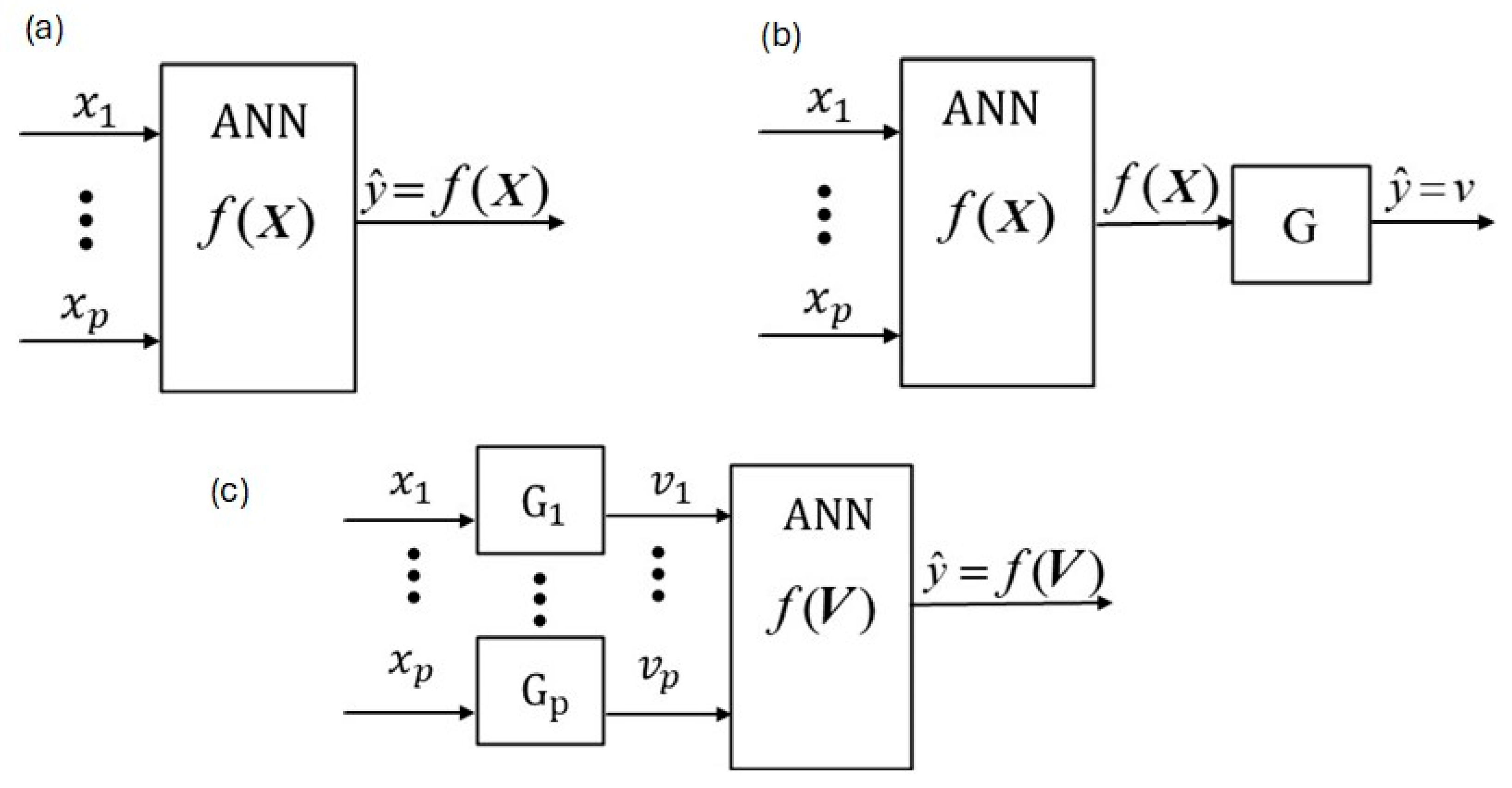
Figure 2.
Diagram of PINN network from [51].
Figure 2.
Diagram of PINN network from [51].
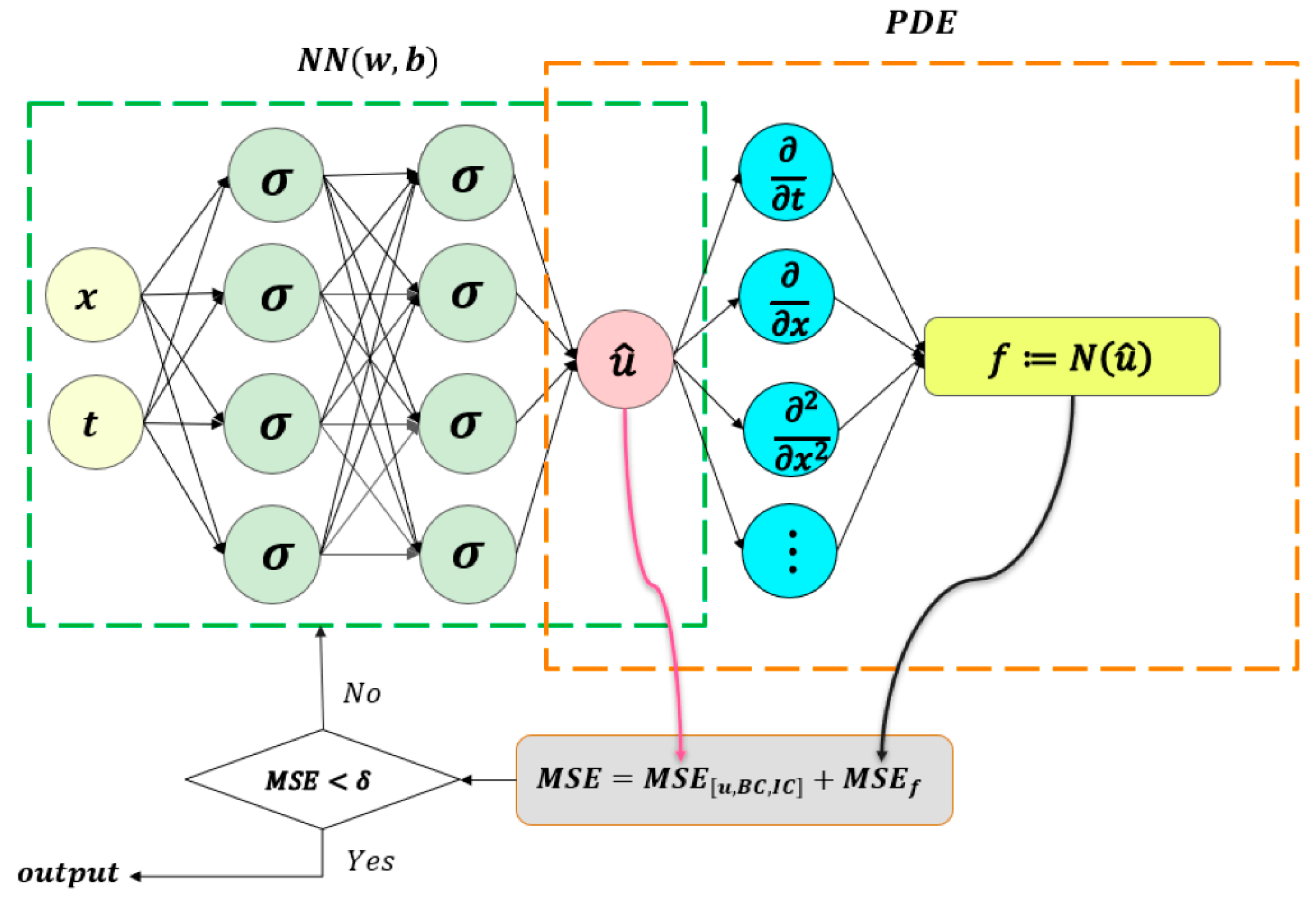
Figure 3.
Python® Stage 2, Model 1, Observed and Fitted, Training and Validation graphical results.
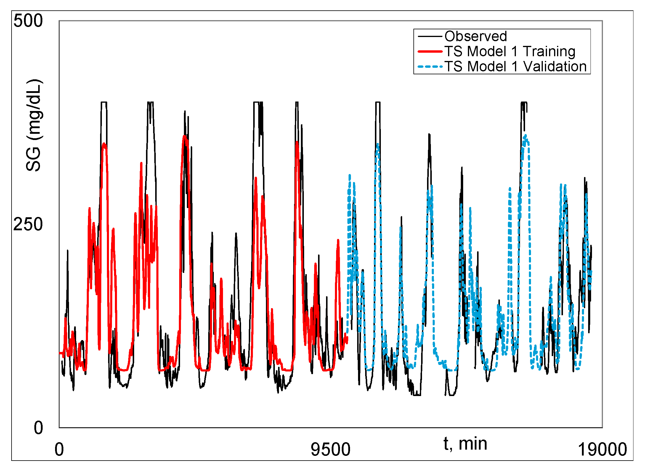
Figure 4.
Python® Stage 2, Model 2, Observed and Fitted, Training and Validation graphical results.
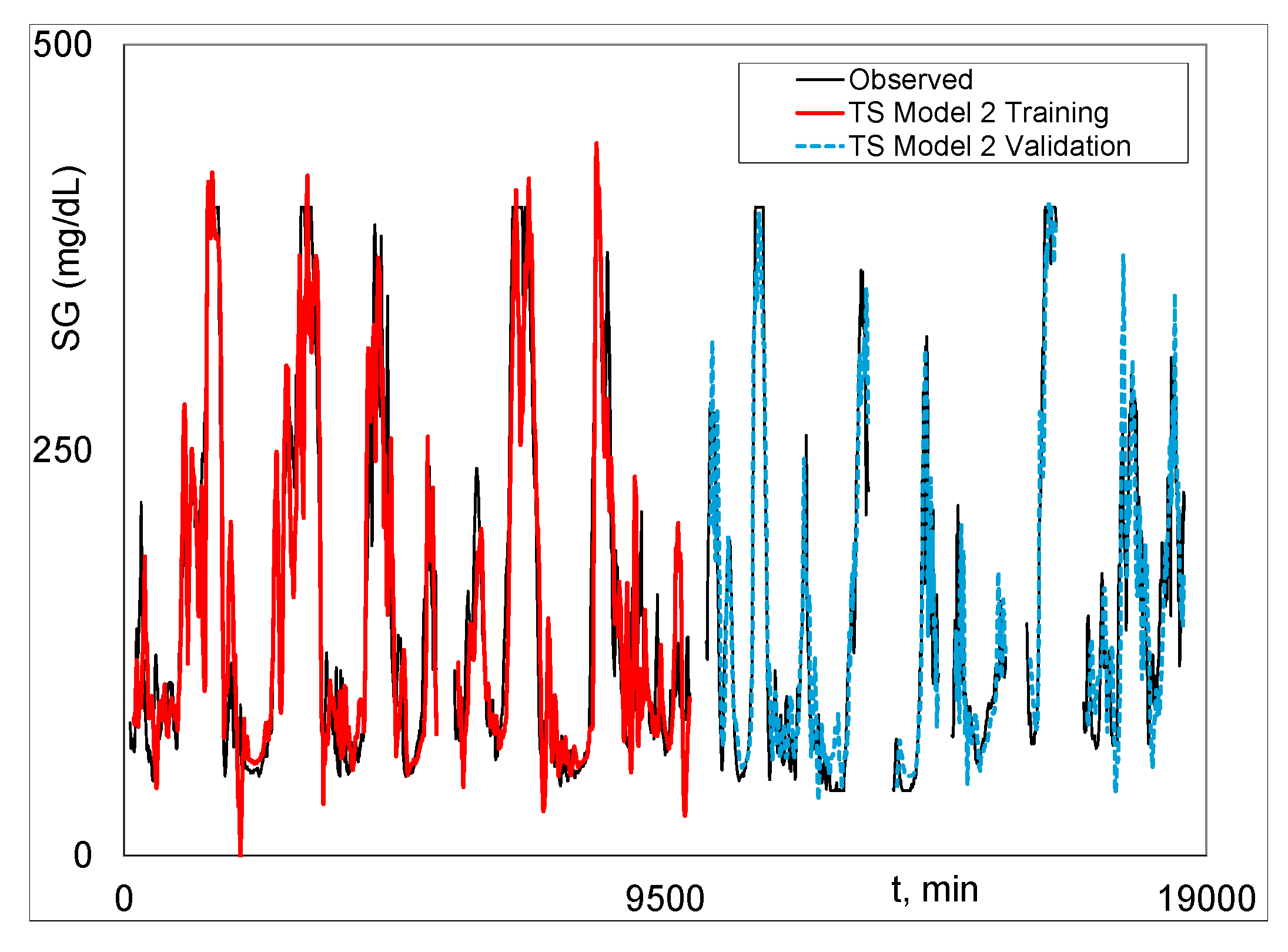
Figure 5.
Python® Stage 2, Model 1-2, Observed and Fitted, Validation graphical results.
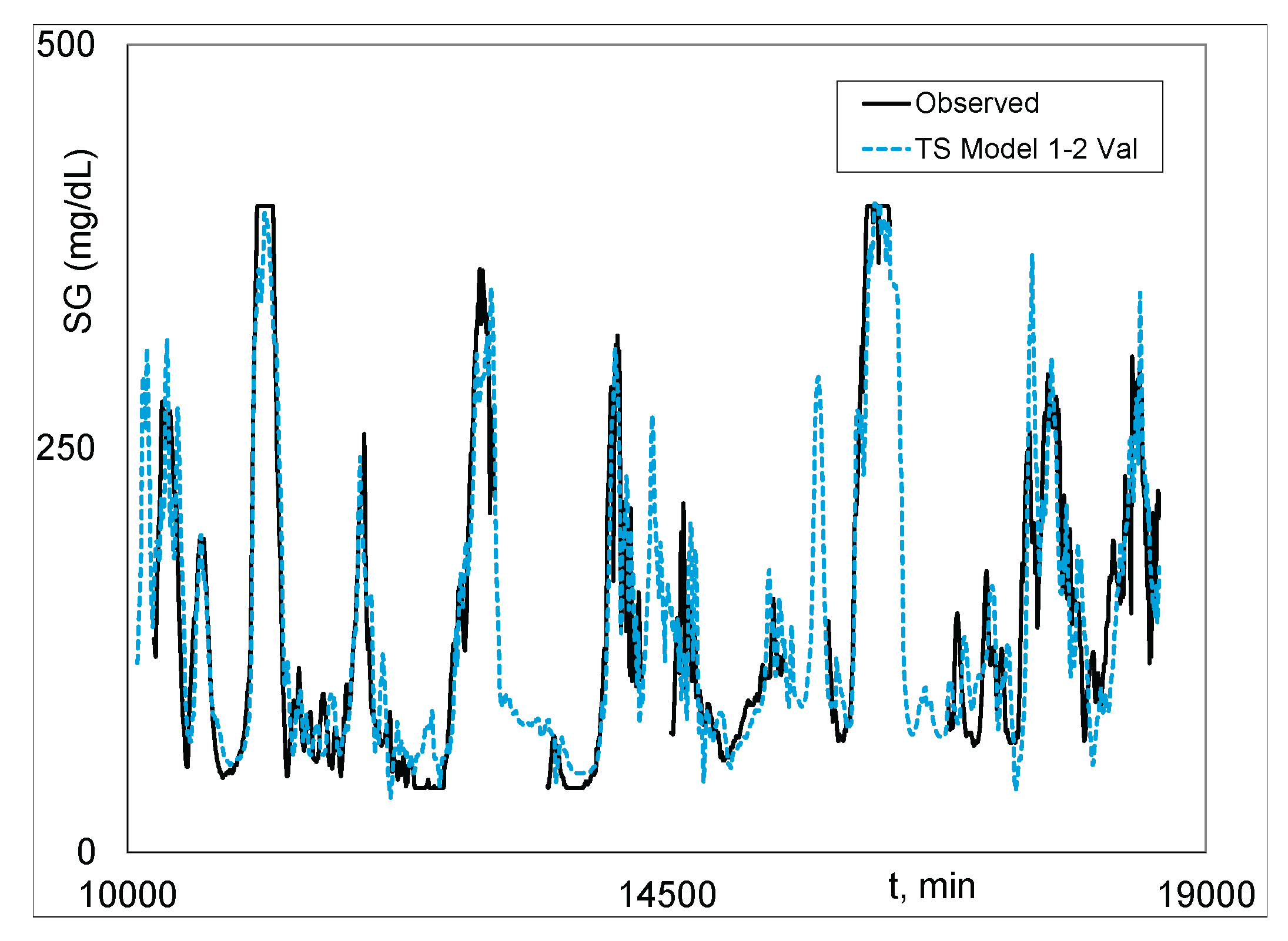

Table 1.
Stages 1 and 2 Modeling Results 1.
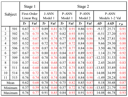 |
| 1 All results are rfit unless otherwise indicated. Stage 1 results are for Model 1. J-ANN means JMP® ANN and P-ANN means Python® ANN. |
Disclaimer/Publisher’s Note: The statements, opinions and data contained in all publications are solely those of the individual author(s) and contributor(s) and not of MDPI and/or the editor(s). MDPI and/or the editor(s) disclaim responsibility for any injury to people or property resulting from any ideas, methods, instructions or products referred to in the content. |
© 2025 by the authors. Licensee MDPI, Basel, Switzerland. This article is an open access article distributed under the terms and conditions of the Creative Commons Attribution (CC BY) license (http://creativecommons.org/licenses/by/4.0/).
Copyright: This open access article is published under a Creative Commons CC BY 4.0 license, which permit the free download, distribution, and reuse, provided that the author and preprint are cited in any reuse.


