
Submitted:
04 October 2025
Posted:
06 October 2025
Read the latest preprint version here
Abstract
We present a model of reality in which worldlines flow between the Universe and an Antiverse, as well as their time-reversed counterparts, and back by passing through black hole singularities. The model is formed by expressing the FLRW metric in Kruskal-Szekeres coordinates and noting that this gives us two Big Bang singularities that are colocated with the Schwarzschild singularities on the Kruskal-Szekeres coordinate chart. By further showing that comoving worldlines in the interior Schwarzschild metric lie on a circular arc, we show that the interior Schwarzschild manifold curves away from the FLRW/Extrior Schwarzschild manifolds. The FLRW/Exterior Schwarzschild manifolds are shown to be tangent to the circular interior Schwarzschild manifold with the event horizon being the point of contact between the manifolds. This geometry provides a path through which particles can cycle between the Universe, a time-reversed Universe, an Antiverse, a time-reversed Antiverse, and back to the Universe by passing through Black Holes and emerging from White Holes.
Keywords:
general relativity
; cosmology
; FLRW
; black holes
; singularities
1. Introduction
The Big Bang and Schwarzschild singularities are two of the most mysterious objects in General Relativity. One of the big questions associated with these singularities is: What happened before the Big Bang and what happened after the Schwarzschild singularity?
When the Schwarzschild metric is expressed in Kruskal-Szekeres coordinates, we see that there are actually two singularities in the metric. By similarly expressing the FLRW metric in Kruskal-Szekeres coordinates, it will be shown that the FLRW metric also has two singularities, which are colocated with the Schwarzschild singularities. But under closer inspection, we find that even though the singularities are colocated on that coordinate chart, they are not colocated in spacetime. Instead, we find that the interior Schwarzschild manifold curves away from the FLRW/Exterior Schwarzschild manifold and they intersect at the event horizon.
Once this geometry is made clear, it becomes clear that there is more to these manifolds than is currently known. In particular, it becomes clear that there is a separate, ’parallel’ time-reversed Universe in which White Holes are the source of matter and the FLRW singularity is the sink into which this time-reversed universe collapses.
In the end, we are able to chart a path between all the singularities and what emerges is an eternal cycle that is powered by Black and White Holes.
2. Transforming the Coordinates of the FLRW Spacetime
The flat FLRW metric is typically given in the following form:
In this paper, we will focus on the and terms in the metric and mostly ignore the azimuthal term. We wish to express the metric in Kruskal-Szekeres coordinates in order to compare the Schwarzschild and FLRW singularities. The first step is to express the FLRW metric in a form that resembles the Schwarzschild metric. We do this by changing the time coordinate:
And from this we see that:
Since we have as a function of t, we can express the scale factor a as a function of instead of t and rewrite the flat FRW metric as (without the angular term):
Contrast this with the interior Schwarzschild metric given below:
Now, it is important to keep in mind that in the interior Schwarzschild metric, r is the timelike coordinate and t is the spacelike coordinate, which is opposite to the FLRW coordinate labels.
Comparing Equations (4) and (5), we see that (when ignoring the angular terms), they have the same form with a time-dependent scale factor multiplying the spacelike coordinate and the inverse of the scale factor multiplying the timelike coordinate. This is interesting because the Schwarzschild metric, when expressed in Kruskal-Szekeres coordinates, is shown to have two ’branches’ in its geometry. In Schwarzschild coordinates, the Schwarzschild metric has an exterior solution and an interior solution. In Kruskal-Szekeres coordinates, we get an additional exterior region and an additional interior region, as can be seen in the Kruskal-Szekeres coordinate chart below [1]:
So the metric in Schwarzschild coordinates gives regions I and II in Figure 1 and when converting to Kruskal-Szekeres coordinates, we get the additional regions III and IV. Since the metrics have such similar structures, we’d like to see if we can get an additional branch for the flat FRW metric by doing a similar coordinate transformation for that metric.
We will define the new coordinates for the FRW metric as follows:
where is a constant with units of time. Our goal is to find the function for the FLRW metric. If we take the differentials of T and X we get:
where is . Next, we find :
Next, we assume the metric in these coordinates will have the form:
Comparing Equations (8) and (9) with Equation (4), we can derive the constraints we need to determine and . First, we recognize that:
And,
If we substitute Equation (11) into Equation (10), we get the following differential equation for :
Equation (12) is a differential equation that allows us to solve for given .
Let us first consider the matter-dominated FLRW Spacetime. In t coordinates, we know that . We can make this an equality with the constant such that . We can integrate this to obtain as a function of t per Equation (3). The integration gives us:
With this, we can obtain the scale factor as a function of :
Plugging Equation (14) into Equation (12), we can solve the function :
We can repeat the same procedure for the radiation-dominated case where and therefore . In this case, . Solving for a we get the following:
And the solution for with the radiation-dominated scale factor is:
And can be found for each case using Equation (11).
We can give the general formulas for and for scale factors of the form :
The full metric in these coordinates is given by:
So we have successfully found Kruskal-Szekeres equivalent coordinates for the FLRW metric. The coordinate chart can be constructed from:
And perhaps more importantly:
An important thing to note here is that when , corresponding to the Big Bang singularity of the FLRW metric, and therefore for that time. This is the same location on the coordinate chart as the Schwarzschild singularity.
So from this analysis, we have found two important facts:
- By expressing the FLRW metric in the Kruskal-Szekeres coordinates, we find that it has two distinct branches, just like the Schwarzschild mertic
- Both the Schwarzschild and FLRW singularities are hyperbolas at in the Kruskal-Szekeres coordinatess
3. Mapping Worldlines from the Big Bang to the Schwarzschild Singularity
We have found that the FLRW and Schwarzschild singularities are both found at the same location on the Kruskal-Szekeres coordinate chart. We must now try to understand how these manifolds are related by trying to map a worldline from the Big Bang to the Schwarzschild singularity.
Even though these singularities can be placed at the same location on the Kruskal-Szekeres coordinate chart, it seems unlikely that they both correspond to the same location in spacetime, so we first need to understand how these singularities are related.
A clue to this comes from calculating the proper time of a co-moving () observer from the event horizon to the singularity. We do this by setting in Equation (5) and integrating from to . This integral gives us:
We recognize this as the length of the arc of a quarter of a circle with radius . This seems unlikely to be a coincidence. What this tells us is that the interior Schwarzschild metric manifold has a circular curvature, meaning that when falling through time from the event horizon in the interior metric, the comoving observer travels along a circular arc with radius . This can explain how the Big Bang and Schwarzschild singularities can be located at the same T in the Kruskal-Szekeres without actually intersecting in spacetime. We can imagine the manifold containing the Big Bang singularity and event horizon lying on a plane, while the manifold of the interior metric curves away from that plane going from the event horizon to the singularity. A depiction of worldlines going from the Big Bang to the Schwarzschild singularity from both branches of the Kruskal-Szekeres coordinate chart is given in Figure 2.
Let us break down Figure 2. First, we will refer to the second branch of the Schwarzschild and FLRW metrics on the Kruskal-Szekeres coordinate chart as the ’Anitverse’ to distinguish it from the Universe. On the left side of Figure 2, we see the curvature of the interior manifold. This Interior View is like looking at the lines in regions II and IV of Figure 1 on a plane perpendicular to the page at .
The upper left arc represents region II in Figure 1 and the lower right arc represents region IV. The point at the center of the ’Interior View’ on the left side of the diagram is the point of Figure 1, which is unreachable because it is outside the manifold, but is the center around which the manifold is curved. The top and bottom dots at the center of the Interior View represent a point on the event horizon of the black hole in the Universe and Antiverse. The points on the left and right at the center of the Interior View represent the Schwarzschild singularities. The points in the top left and bottom right of the Interior View are the Big Bang singularities of the Universe and Antiverse. This view illustrates how the singularities can overlap on the Kruskal-Szekeres coordinate chart without actually intersecting in spacetime.
Looking at the Exterior View on the right side of the diagram, we are now looking at a ’top-down’ representation of the manifold containing the Big Bang singularities and event horizons. The three points in this view represent the same FLRW singularities and event horizons depicted in the interior view; we are just looking at them on the manifold that is oriented 90 degrees relative to the interior manifold.
So there are examples of two worldlines exiting the FLRW singularities in the Exterior View. The straight worldline represents the worldline of particles that never fall into a black hole and escape to infinity or the ’heat death’ of the Universe. The curved line represents the path of a particle that falls into a black hole. So, the way to look at this is to follow the curved line from the FLRW singularity to the center point of the Exterior View diagram which represents the event horizon. At that point, we move to the Interior View where the particle is at the top of the diagram for particles from the Universe and at the bottom of the diagram for particles from the Antiverse. These particles then fall to their respective singularities on the left and right sides of the view.
But these diagrams are practically screaming out to be completed. In particular, when we look at the interior view, one cannot help but feel like the circle needs to be completed. The circle can also be completed if we include time-reversed scenarios. Time-reversing the process involves swapping the functions of the singularities. In the time-forward case, the FLRW singularity is a source and the Schwarzschild singularity is a sink. In the time-reversed case, the FLRW singularity is a sink, and the Scbhwarzschild singularity is a source.
In the time-reversed case of the Interior View, matter would emerge from the singularity and move to exit the event horizon. In the time-reversed case of the Exterior View, particles would emerge from white holes and move toward the FLRW singularity as the Universe collapses. We can show that once the Schwarzschild singularity is reached, time reversal is possible by examining the mathematics of the Kruskal-Szekeres coordinates for the interior metric.
Equation (24) is the definition of the T coordinate in terms of the Schwarzschild coordinates for the interior metric:
For a comoving observer, the Equation (24) has a constant t and r is the time coordinate, so we can define the velocity of the frame in T as:
We take the negative solution for region II of the Kruskal-Szekeres coordinate chart since T increases when r decreases there. We can see that this velocity is when and zero when . So, the velocity is zero at the singularity. If we take the derivative of this velocity, we get:
Since is negative, this tells us that will be positive from to . But is negative and, therefore, the acceleration of the worldline is opposite to the velocity, causing it to decelerate in T and therefore the acceleration vector would point towards . We can also see that this acceleration is non-zero at the singularity. So if is 0 at and the derivative of is nonzero and points toward at , then this means that after approaching the singularity from the worldline stops moving in increasing T at the singularity and begins to move in the direction of decreasing T. When the worldline then starts to fall back towards , is still negative, but is now positive. Thus, will be negative, which means that the worldline accelerates toward the event horizon.
So, let us add the time-reversed worldlines to Figure 2 and interpret the results. Figure 3 adds the time-reversed processes with labels describing each process and numbers labeling important junctions.
Let us go through the process step-by-step starting at step 1, which is a particle leaving the Big Bang:
- Particle emerges from the Big Bang in the time-forward Universe
- Particle crosses the event horizon in the time-forward Universe
- Particle reaches the Schwarzschild singularity in the time-forward Universe and is spagghettified
- Particle emerges from the Schwarzschild singularity in the time-reversed Universe
- Particle emerges from the white hole in the collapsing time-reversed Universe
- Particle reaches the Big Bang singularity in the collapsed time-reversed Universe
- Particle emerges from the Big Bang in the time-forward Antiverse
- Particle crosses the event horizon in the time-forward Antiverse
- Particle reaches the Schwarzschild singularity in the time-forward Antiverse and is spagghettified
- Particle emerges from the Schwarzschild singularity in the time-reversed Antiverse
- Particle emerges from the white hole in the collapsing time-reversed Antiverse
- Particle reaches the Big Bang singularity in the collapsed time-reversed Antiverse
- Cycle begins again
Of note here is that we end up with four different universes through which the worldlines cycle. So when the particles emerge from the Schwarzschild singularities, they do not move back in time in the Universe; they move forward in time in a separate time-reversed Universe. We also see that the collapsing time-reversed Universe and Anitverse feed into the Big Bangs of the time-forward Antiverse and Universe.
We can see from the diagrams that the time-forward Universe and time-reversed Antiverse move in the same direction of time and the time-forward Antiverse and time-reversed Universe move in the same direction of time. But those two directions are opposite to each other. Therefore, we can conjecture that the time-forward Universe and time-reversed Antiverse contain mostly matter and the time-forward Antiverse and time-reversed Universe contain an equal amount of mostly antimatter. This would mean that the Schwarzschild singularities convert matter to antimatter and antimatter into matter.
There are still two outstanding problems that need to be addressed. First, in Figure 3, when looking at the Interior View, we have an FLRW Universe and time-reversed Antiverse in the top left quadrant, and an FLRW Antiverse and time-reversed Universe in the lower right quadrant, but nothing in the other two quadrants (in the Exterior View, the left half of the diagram is actually on an upper plane, while the right half of the diagram is on a lower plane). But more importantly, when the particles come out of the Schwarzschild singularity, they can exit from one of two horizons into the time-reversed spacetimes, not just a single horizon as has been implied.
Both of these issues can be solved by adding a second set of 4 spacetimes (Universe, Antiverse, time-reversed Universe, and time-reversed Antiverse) but with their parity flipped relative to the original 4. So, the Universe and time-reversed Antiverse with flipped parity would be in the top right quadrant of the Interior View of Figure 3 with the heat death vector pointing up on the right side of the Exterior View. The Antiverse and time-reversed Universe with flipped parity would likewise go in the bottom left quadrant. The parity-flipped Exterior View is shown in Figure 4 below.
We can also see how this solves the problem of particles exiting the singularity having a choice of two paths by looking at the worldlines on the Kruskal-Szekeres coordinate chart in Figure 5 below.
In these diagrams, we place the FLRW singularities at infinity at and the same numbers used to enumerate the cycle in Figure 3 are labeled in this figure. On the left side, we show the full cycle described in this paper. On the right, we have the parity-flipped cycle. If we focus on the path from point 4 to 5, where the particle emerges from the Schwarzschild singularity and then emerges from a white hole in the time-reversed Universe, we see that if it exits the left horizon (as is the case in the left diagram), it will enter a time-reversed Universe with the same parity as the original Universe from which it came. But if it exits the right horizon then it enters a time-reversed Universe whose parity is flipped relative to the original Universe.
When particles leave the singularity, they have an equal chance of going in either direction because they will emerge from the singularity along a line of constant t. We can see this by looking at the geodesic equation for the t coordinate of the interior metric:
While the particle falls toward the singularity, is negative, since r decreases from to during the fall. This means that the acceleration in t is always opposite to the velocity . And we see that at , Equation (27) is infinite, so the particle’s velocity in t is forced to 0 as it reaches the singularity. If it enters the singularity with constant t, it will exit with constant t. And since we are free to hyperbolically rotate the t coordinates on the Kruskal-Szekeres chart without changing anything, whichever t the particle reaches the singularity at we can rotate to such that the particle emerges from the singularity moving straight down along the axis in region II of the coordinate chart and from there with an infinitessimal nudge in either direction of t it will go toward one horizon or the other.
So time forces the particle to move from Universe to time-reversed Universe to Antiverse to time-reversed Universe and back to Universe. The particle has no choice in this because it must move forward in time. But the particle can choose the parity of the Universes it transitions to by choosing a direction in space while exiting the interior metric.
Figure 3 and Figure 5 also help us understand the nature of the Schwarzschild and FLRW singularities. All the points on the worldlines between 1 and 3, 4 and 6, 7 and 9, 10 and 12 have a known direction of time (you can specify the direction in which time flows on those lines). But at the singularities, the direction of time is undefined. For a particle at either of the FLRW or Schwarzschild singularities, the particle cannot know if it is in a time-forward or time-reversed spacetime (Schwarzschild singularities move particles from time-forward to time-reversed and FLRW singularities move particles from time-reversed to time-forward spacetimes) because time is essentially undefined at the intersections of these spacetimes.
We can update the interior Schwarzschild metric to use an angular coordinate for the time coordinate instead of r. We can say that for a co-moving observer, and we know that for this observer, . Therefore, we can rewrite the interior Schwarzschild metric as:
4. Inside the Horizon: From Matter to Antimatter
It has been claimed here that when a particle exists the Schwarzschild singularity, it exits with a charge opposite to what it entered the singularity with. Let us put this on firmer footing by carefully considering what a person falling in a black hole would experience and how they would be able to move while inside the black hole.
Figure 6 depicts Scout falling into a black hole, passing through the singularity, and exiting the white hole. Figure 6 below.
On the left side of the picture, we see a depiction of Scout falling into a black hole, passing the singularity, and then exiting the white hole. On the right, we see example worldlines representing a point at the top of Scout’s head and a point at her feet where the two points lie on the same radial line of the black hole (note that in Section 5, we will show that the depiction of Scout in Figure 6 is not accurate, but is useful for the current discussion).
What would Scout see when looking up and down while falling? Well, if she looked up, she would just continue seeing light come in from the outside Universe, just as she did when she was in the exterior metric (i.e. it would still look to her like she was in the exterior metric). However, when she looks down, she will not see empty darkness. We said that the t coordinate is related to when something fell into the black hole relative to the first thing(s) that created the black hole. Consider a black hole formed from a collapsing shell. The material from the shell would be the first thing that ’falls in’ to the black hole, so we will place its worldline on the Kruskal-Szekeres chart along , as shown in Figure 7.
If Scout is the next thing to fall into the black hole sometime later, we see her worldline to the right of the shell’s line in the center. The dashed lines show the light that Scout will see as she falls, and she is seeing the shell collapsing below her for the entire time she’s falling. What this means is that someone falling into a black hole never sees the singularity, they will always see whatever fell in before them the whole way down, no matter when they fall in relative to when the black hole was created. Even just before Scout reaches the singularity, she never sees the shell reach the singularity, which is seen by the fact that the last dashed line that intersects Scout’s line at the singularity connects to a past point on the shell’s worldline.
Now imagine that Scout is spinning about her central radial axis as she is falling. The spin is depicted in Figure 6 with the arrows pointing radially and going through Scout’s centerline. So, we see that when she falls toward the singularity, her spin vector is pointing toward the horizon, but as she moves away from the singularity after crossing, the spin vector is pointing in the opposite direction. The important thing here is that she is spinning around a radial axis, and that axis is timelike. If instead of thinking of Scout spinning, we consider a quantum particle, we could conjecture from this that electric charge comes from a quantum particle’s intrinsic spin around the timelike dimension, whereas the normal quantum spin comes from intrinsic spin around spacelike axes.
If this conjecture is true, then we immediately see why matter is turned to antimatter (and vice versa) after passing through the singularity. The spin axis goes from pointing toward/away from the singularity to pointing opposite after it passes. So, if Scout were a quantum particle, she would be a matter particle that turned into an antimatter particle after passing the singularity because the orientation of her charge spin vector was reversed after crossing the singularity. This is because if, from the perspective of someone outside the black hole looking down on Scout as she fell into the black hole saw her spinning counterclockwise, she would be spinning clockwise from the perspective of someone outside the white hole when she emerged.
The charge being the spin of the particle about its timelike dimension also helps us to understand things like how a moving charge creates a magnetic field. When a charged particle moves with some velocity in the lab frame, its inertial frame is boosted relative to the lab frame. Thus, the particle’s time axis has a projection onto the space-like axis of motion in the laboratory frame. This means that the charge spin vector has a projection on this axis, which behaves like regular quantum spin, and quantum spin is well known to give the particle an intrinsic magnetic field.
5. Transiting the Singularity
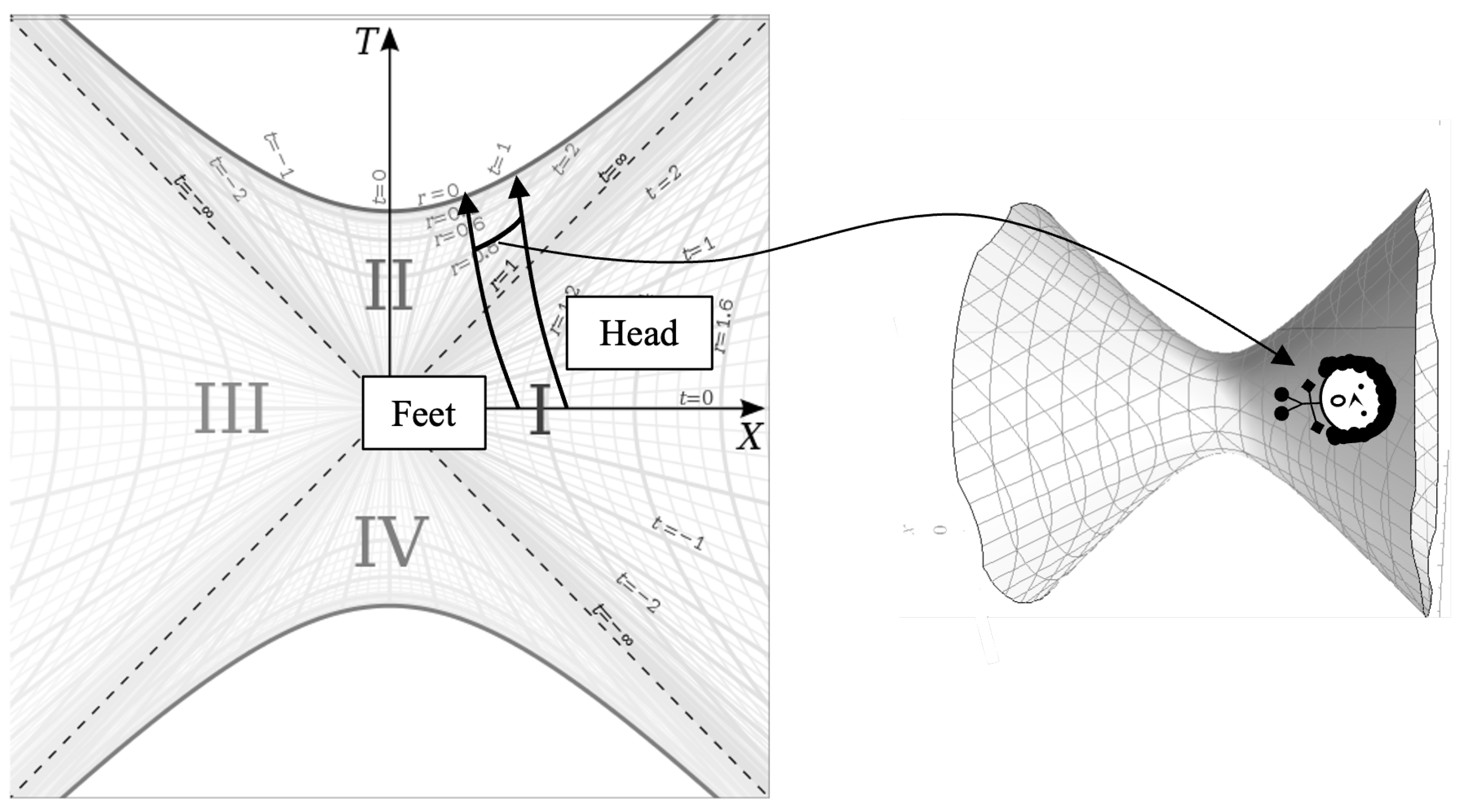
Let us now consider Scout’s traversal of the singularity. The common understanding is that as Scout reaches the singularity, she will be squeezed around her radial axis and stretched along it. However, we can show that this is not the case. In fact, every point on the Scout’s body will be preserved at just as it is at any other r. Figure 8 shows this in 2D.
On the left, we have the worldlines of Scout’s head and feet again and we show an arc of constant r between them. That arc represents all of Scout’s points lying along her centerline at the time r corresponding to that hyperbola. If we take slices of Scout from her left to her right, then each slice is a fixed and each point on a given slice is a fixed t.
On the right of Figure 8, we have swept the hyperbola around , which we will define as the direction to create the 2D surface of t and on which Scout is (it is actually a 3D volume, but we can only depict the 2D surface). So, as we can see, all of Scout is shown on the manifold, even though we are looking at a single value of r.
But we can make the exact same hyperboloid at and draw Scout on the surface exactly as we did in Figure 8. So, even though the angular dimensions have collapsed at , there is still an infinite hyperbolic t axis in every direction at . This means that there is an infinite 3D volume at that can preserve the positions of particles on the manifold relative to each other. The proper distance between t coordinates goes to infinity at because, as was shown with Equation (27), must be zero there and so there cannot be motion in t at the singularity. But anything separated in the azimuthal directions will be connected by null geodesics at the singularity. But we are separated from everything we see by null geodesics. The difference here is that the null geodesics we are accustomed to separate the objects in both space and time. At the singularity, they only separate things in space at the same time.
This exercise shows us that our depiction of Scout in Figure 6 is incorrect. As she crosses the horizon, Scout changes from occupying space in the r dimension to occupying space in the t dimension. So, rather than falling as shown in Figure 6, when she is in the interior, she would be on a surface like that shown in Figure 8 at each r over time as opposed to being spread out over time.
Therefore, we have shown that it is possible, in theory, to transit the Schwarzschild singularity without being destroyed or ’spaghettified’.
6. Conclusions
We have presented a model of reality in which worldlines cycle endlessly between a Universe and an Antiverse as well as their time-reversed counterparts. The Schwarzschild black holes act as engines shuttling particles between these Universes, converting matter into antimatter and vice versa in the process.
Though some particles may escape the cycle to heat death, which is like the exhaust of an engine, since the universes are spatially infinite and therefore contain infinite matter/antimatter, there will always be an infinite amount of particles going through the cycle (if 1 in X particles fall into a black hole each cycle, an infinite amount of particles will fall into a black hole no matter how large X is since the cardinality of the set of particles is infinite). The cycle is therefore eternal, with no beginning or end. This is also a continuous cycle, meaning that there is material that continuously flows through the cycle. We also know that cycles do not repeat since some particles will always be vented to heat death. This means that the specific particles being cycled are always changing and that "whenever" one looks at the Big Bang, they would see different particles emerging.
We only considered non-rotating black holes in this analysis, but for the more realistic case of rotating black holes, the ring singularity may alter the experience of falling through the center of the black/white hole. We can surmise, however, that just as the Universe has rotating black holes, this implies that the time-reversed Universe must have rotating white holes. A more thorough investigation of the rotating black hole scenario will be left for future research.
Data Availability Statement
All data generated or analyzed during this study are included in this published article [and its supplementary information files.
Conflicts of Interest
There are no competing interests.
References
- Figures 1 and 3 are modifications of: ’Kruskal diagram of Schwarzschild chart’ by Dr Greg. Licensed under CC BY-SA 3.0 via Wikimedia Commons. http://commons.wikimedia.org/wiki/File:Kruskal_diagram_of_Schwarzschild_chart.
Figure 1.
Kruskal-Szekeres Coordinate Chart
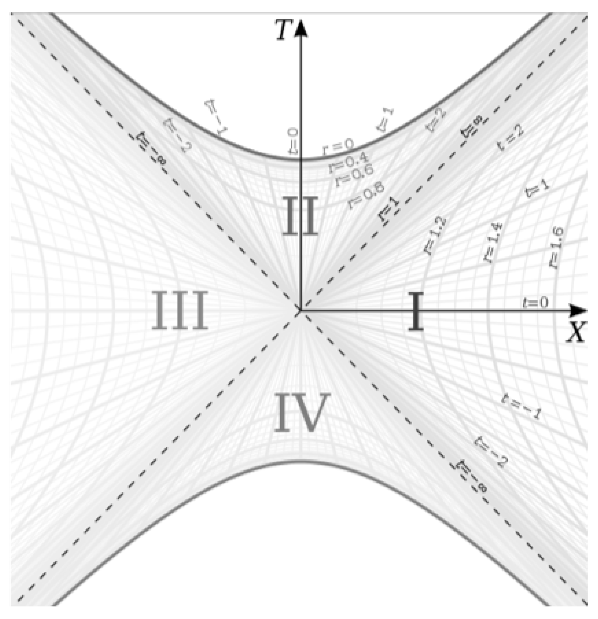
Figure 2.
Map of Worldlines from the Big Bang to the Schwarzschild Singularity
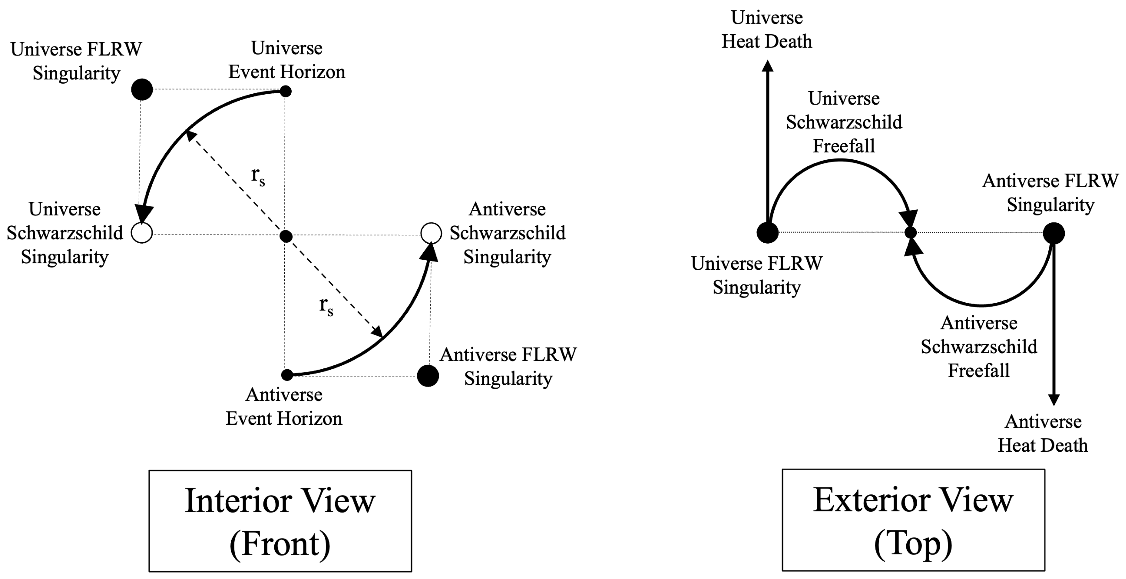
Figure 3.
Map of Worldlines from the Big Bang to the Schwarzschild Singularity with Time-Reversed Processes
Figure 3.
Map of Worldlines from the Big Bang to the Schwarzschild Singularity with Time-Reversed Processes
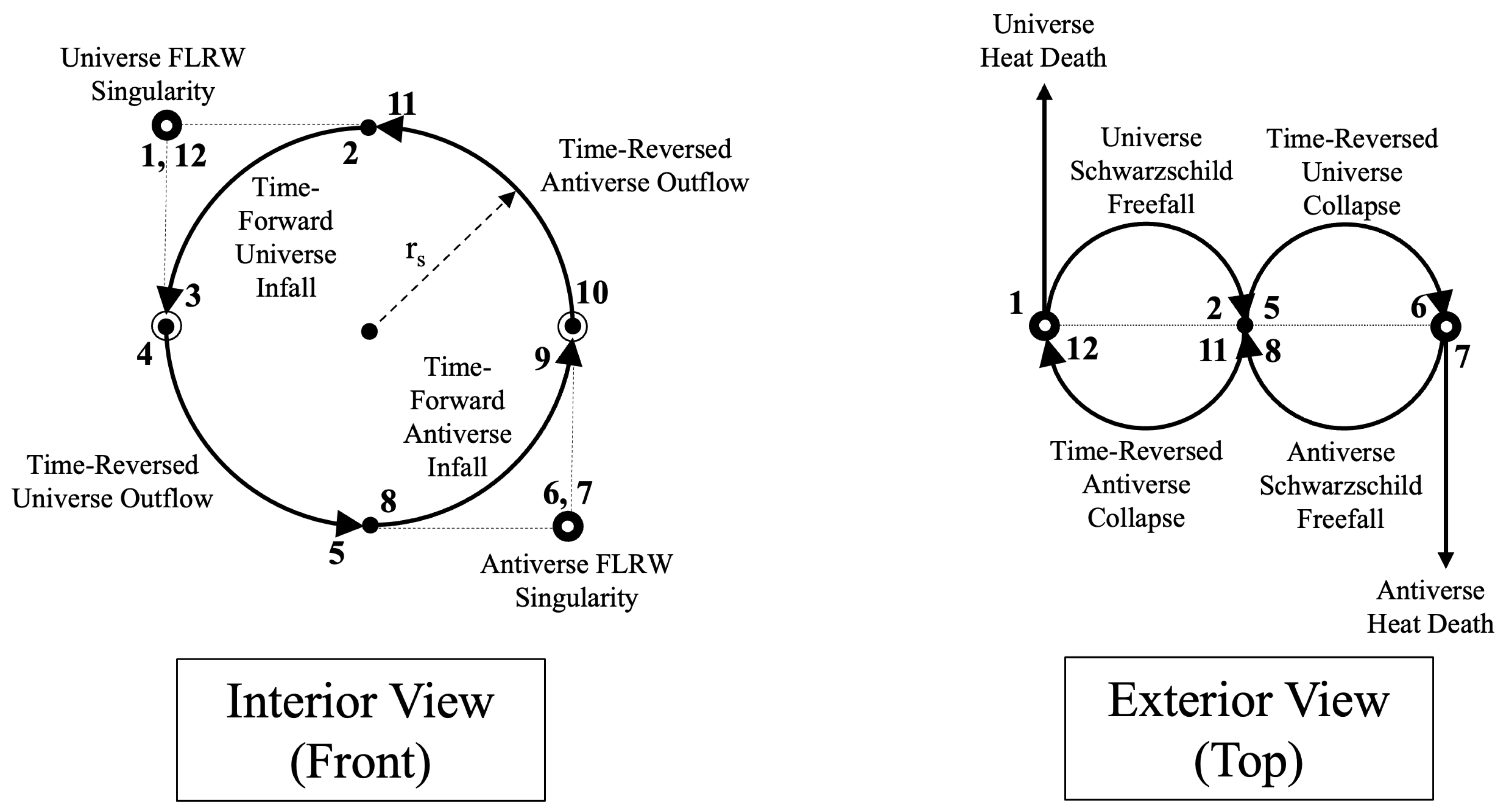
Figure 4.
Parity-Flipped Exterior View
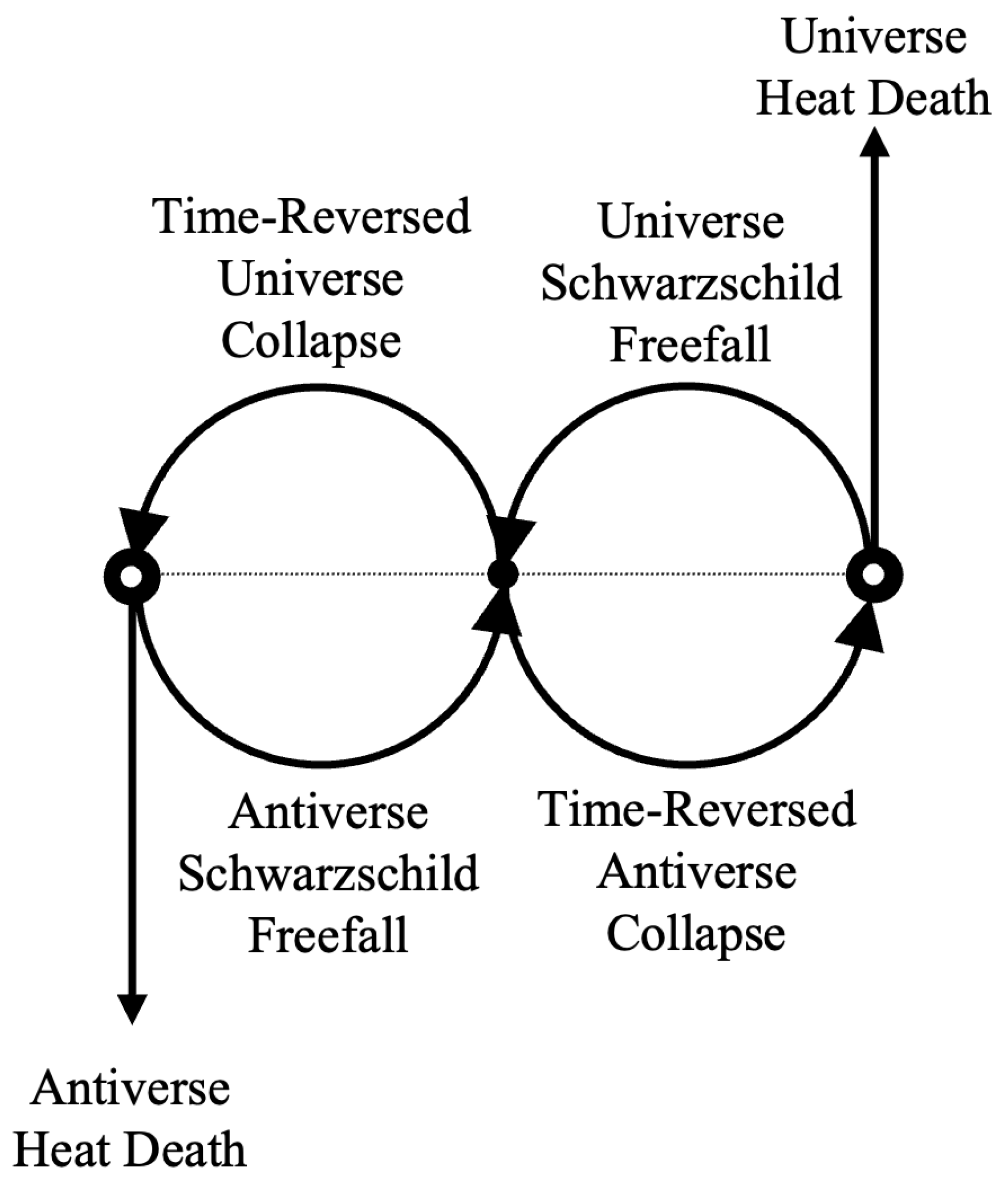
Figure 5.
Normal Cycle (left) and Parity-Flipped Cycle (right)
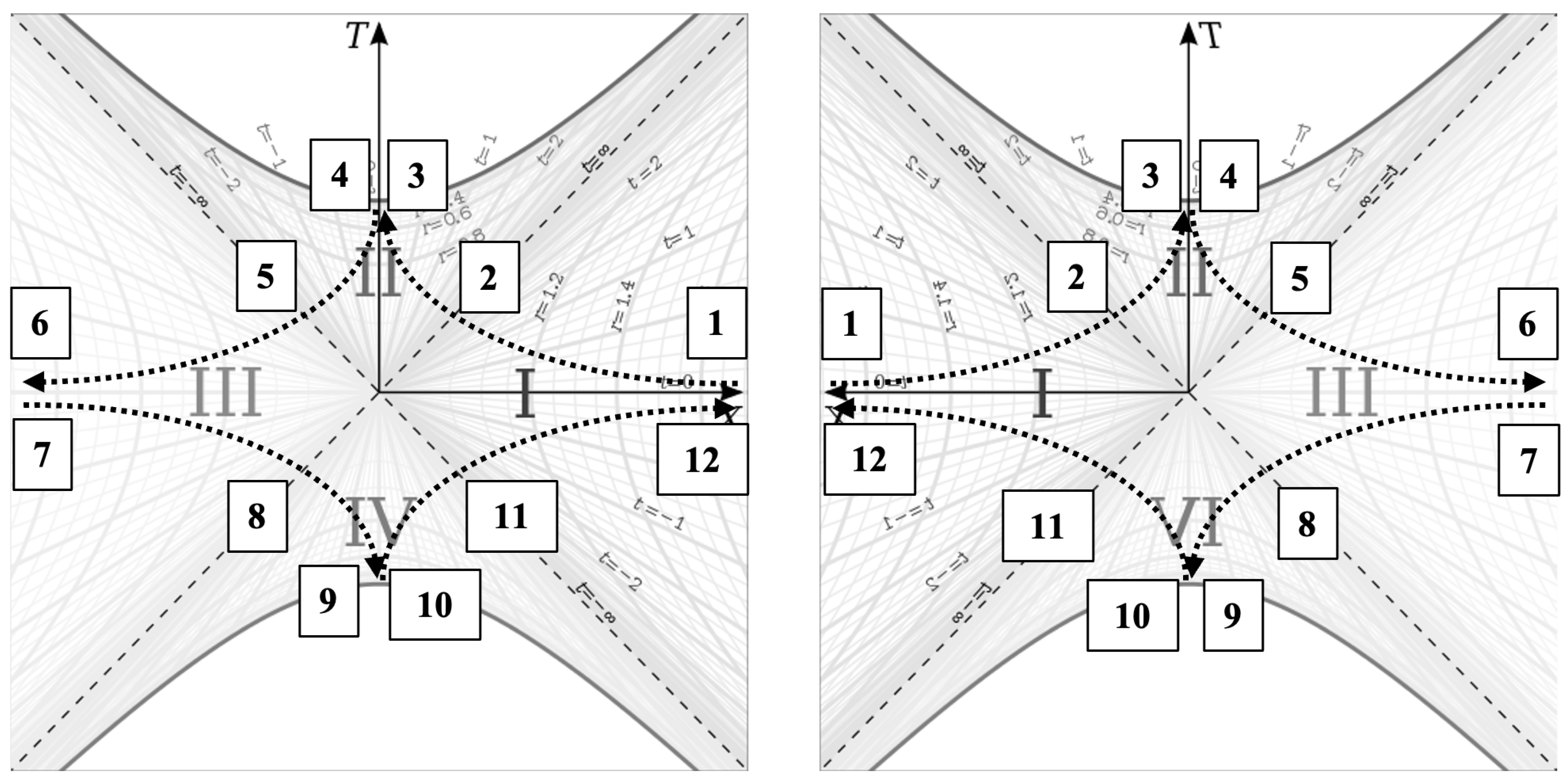
Figure 6.
Scout Falling in a Black Hole and Exiting a White Hole
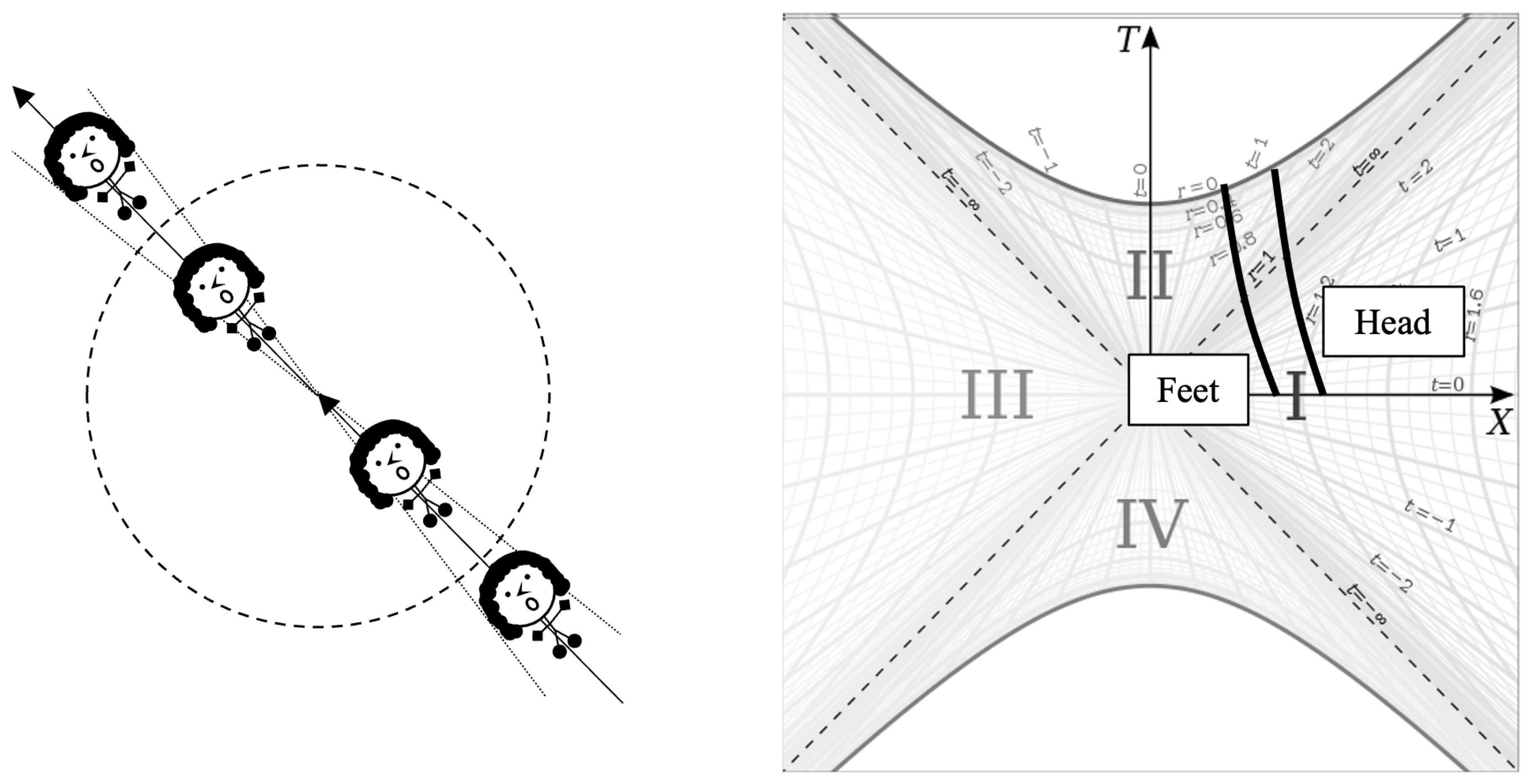
Figure 7.
Scout’s View when Looking Down
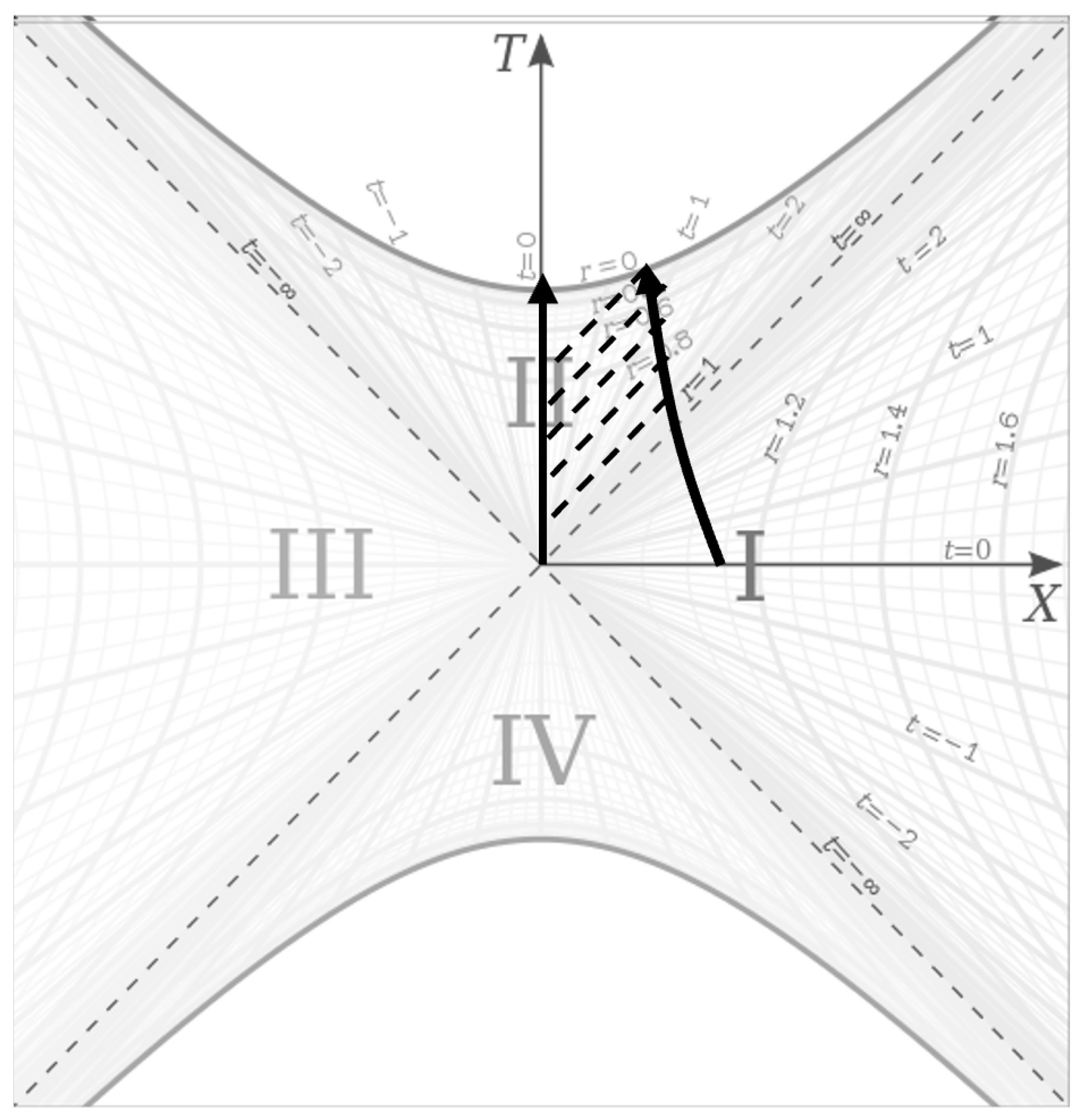
Figure 8.
Scout on the Interior Manifold
Disclaimer/Publisher’s Note: The statements, opinions and data contained in all publications are solely those of the individual author(s) and contributor(s) and not of MDPI and/or the editor(s). MDPI and/or the editor(s) disclaim responsibility for any injury to people or property resulting from any ideas, methods, instructions or products referred to in the content. |
© 1996 by the author. Licensee MDPI, Basel, Switzerland. This article is an open access article distributed under the terms and conditions of the Creative Commons Attribution (CC BY) license (https://creativecommons.org/licenses/by/4.0/).
Copyright: This open access article is published under a Creative Commons CC BY 4.0 license, which permit the free download, distribution, and reuse, provided that the author and preprint are cited in any reuse.


