Submitted:
01 October 2025
Posted:
06 October 2025
You are already at the latest version
Abstract
The Hybrid energy storage system (HESS) that combines battery with hydrogen storage exploits complementary power/energy characteristics, but most studies optimize capacity and operation separately, leading to suboptimal overall performance. To address this issue, this paper proposes a bi-level co-optimization framework that integrates deep reinforcement learning (DRL) and mixed integer programming (MIP). The outer layer employs the TD3 algorithm for capacity configuration, while the inner layer uses the Gurobi solver for optimal operation under constraints. On a standalone PV–wind–load-HESS system, the method attains near-optimal quality at dramatically lower runtime. Relative to GA+Gurobi and PSO+Gurobi, the cost is lower by 4.67% and 1.31%, and the runtime is 0.52% and 0.58% of theirs, respectively; compared with a direct Gurobi solve, the cost remains comparable but the runtime is 0.07% of its. Sensitivity analysis further validates the model’s robustness under various cost parameters and renewable energy penetration levels. These results indicate that the proposed DRL–MIP cooperation achieves near-optimal solutions with orders of magnitude speedups. This study provides a new DRL-MIP paradigm for efficiently solving strongly coupled bi-level optimization problems in energy systems.
Keywords:
hybrid energy storage system (HESS)
; hydrogen storage
; battery energy storage system
; co-optimization
; bi-level
; deep reinforcement learning (DRL)
1. Introduction
The Hybrid energy storage system (HESS) integrates power-based energy storage technologies, such as supercapacitors, flywheels, and batteries, with energy-based energy storage technologies, such as hydrogen, thermal, compressed-air, and gravity. This combined approach balances fast power response with long-duration energy supply, addressing the shortcomings of single storage technologies. By adjusting power output across different time scales, HESS improves renewable energy utilization and strengthens the overall stability of energy networks. With properly optimized resource allocation, HESS not only reduces overall system investment costs but also extends the service life of storage devices. Owing to these technical and economic merits, HESS has emerged as a prominent research focus in the energy sector and has been widely deployed in renewable energy systems, active distribution networks, electric vehicles, and integrated energy systems.
Existing studies on HESS optimization primarily focus on three aspects: capacity (sizing) optimization, operation (energy management, scheduling, and power allocation) optimization, and the co-optimization of both capacity and operation. This paper systematically reviews and analyzes the current literature from these three perspectives.
- (1)
- Capacity Optimization
References [1,2,3,4,5] investigated the application of HESS in grid-connected photovoltaic (PV), wind, and wave energy systems, with a focus on capacity optimization to smooth power fluctuations. Reference [6] proposed a multi-objective capacity optimization approach for standalone wind power systems, jointly considering economic performance, reliability, and energy consumption rate. References [7,8] explored HESS deployment in renewable energy systems, optimizing system sizing in response to load demands under varying climatic conditions. Reference [9] examined the role of HESS in islanded microgrids, configuring storage capacity to minimize both overall operating costs and the flexibility-deficiency rate. References [10,11,12,13] focused on integrated energy systems, where capacity optimization of HESS improved system economics and stability while mitigating wind/PV power curtailment and voltage fluctuations.
In summary, HESS capacity optimization models primarily focus on economy, reliability, and equipment operating conditions; however, their operational strategies are mostly rule-based deterministic methods, lacking systematic operation optimization modeling.
- (2)
- Operation Optimization
References [14,15,16] investigated energy management strategies for HESS in electric vehicles, aiming to improve energy efficiency and driving range. References [17,18,19,20,21,22] focused on renewable energy grid-integration scenarios, optimizing energy management to enhance system stability. References [23,24,25,26,27,28,29,30,31,32,33,34,35] explored the optimal operation of HESS in microgrids to achieve global energy management objectives. References [36,37,38] discussed the scheduling optimization methods of HESS in integrated energy systems.
These studies generally assume that storage capacity is predetermined, concentrating instead on optimizing decision variables at the operational level.
- (3)
- Co-optimization of Capacity and Operation
References [39,40,41] addressed the integrated optimization of capacity configuration and energy management for HESS in electric vehicles. References [42,43,44,45,46] explored co-optimization approaches for HESS capacity and operation in multi-energy systems. References [47,48,49,50,51,52,53,54,55] proposed HESS optimization strategies for distributed energy systems, employing bi-level optimization, two-stage stochastic programming, and multi-objective optimization methods to improve system economics and operational flexibility. References [56,57] focused on the collaborative optimization of HESS in microgrids.
Overall, co-optimization of HESS capacity and operation requires coordinating long-term planning with short-term dispatch to optimize decision variables across both dimensions simultaneously.
A review of the above literature reveals that most existing studies treat HESS capacity configuration and operation optimization separately, overlooking the strong coupling between these two aspects. The co-optimization problem can typically be formulated as a mathematical programming model characterized by nonlinear, mixed-integer, and multi-objective properties. The main objective is to simultaneously optimize the capacity and operation strategies of various storage components while meeting constraints such as charging-discharging characteristics, energy balance, system dynamic response, and economic performance. In addition, the intermittent and stochastic characteristics of renewable energy output, along with uncertainties in load demand, further complicate the problem and necessitate a robust model.
Given the close coupling between the planning and operation of hybrid energy storage systems (HESS), determining the optimal configuration in the planning stage and achieving optimal scheduling in the operation stage constitutes a typical bi-level optimization problem. Although this hierarchical structure clarifies the decision-making layer, it also dramatically increases the computational complexity. Specifically, the outer-level optimization focuses on the capacity of the energy storage system to ensure sufficient flexibility for future net-load changes. The inner-level optimization then improves the economy, stability, and reliability of the system by optimizing charging and discharging strategies within predefined capacity constraints. Within this framework, outer-level decisions establish capacity boundaries and allocate resources to the inner level, while the outcomes of inner-level operations, in turn, influence outer-level configuration decisions. This bidirectional interaction necessitates coordinated optimization to achieve system-wide optimality. Although some studies have attempted to optimize both layers simultaneously, the modeling and solution approaches often oversimplify or neglect the dynamic interactions between the two levels.
To address this complex problem, existing solution approaches primarily include mathematical programming, metaheuristic algorithms, and hybrid methods. Mathematical programming approaches (e.g., [40,42,46,51,52,55]) can provide precise and robust optimal solutions but often suffer from limited computational efficiency when applied to large-scale problems. Metaheuristic algorithms (e.g., [39,53]) offer faster solution speeds but struggle to guarantee global optimality. Hybrid methods generally combine heuristic techniques with mathematical programming—such as integrating MOGWO, GA, or PSO with mathematical programming ([41,43,45]) to balance computational efficiency and solution quality. Currently, studies on solving this problem using reinforcement learning and its fusion methods are relatively scarce.
Among various HESS configurations, the lithium-ion battery and hydrogen hybrid energy storage system have gained widespread application in engineering practice due to their pronounced complementary characteristics. Based on this, this paper constructs an HESS that integrates a battery energy storage system (BESS), an electrolyzer (EL), a fuel cell (FC), and a hydrogen storage tank (HST), and applies it to an independent hybrid renewable energy system to improve power supply reliability and economy.
To address the co-optimization of capacity configuration and operation optimization for the HESS, a unified optimization framework is established for solving both problems in an integrated manner. Furthermore, an innovative approach combining reinforcement learning (RL) and mixed integer programming (MIP) was proposed to leverage their respective strengths: RL is well-suited for making sequential decisions in complex, uncertain environments, while MP provides reliable, structured solutions that meet system constraints. Additionally, the model incorporates detailed battery and hydrogen storage degradation characteristics to enhance the model’s accuracy and engineering applicability.
2. System Model
The hybrid energy storage system considered in this paper comprises two subsystems, a lithium-ion BESS and a hydrogen energy storage system. The hydrogen energy storage system consists of an EL, a hydrogen storage tank (HST), and an FC, collectively providing power balancing and energy management services for a standalone hybrid renewable energy system, as shown in Figure 1. The working principle is as follows. Surplus electricity is converted into hydrogen by the electrolyzer and stored in the hydrogen tank; when electricity is required, the fuel cell reconverts the stored hydrogen into power. The lithium battery primarily provides fast, short-term power response, while the two subsystems operate in a complementary manner to achieve multi-timescale energy management.
To achieve the co-optimization of capacity configuration and operational strategy for the lithium-hydrogen HESS, a bi-level optimization model is developed. The core idea is to decompose the comprehensive optimization problem into two interrelated but hierarchical sub-problems. The outer layer deals with capacity configuration (long-term investment decision), and the inner layer addresses operation optimization (short-term dispatch decision). The outer layer determines the optimal capacities of each storage component and provides boundary constraints to the inner layer; the inner layer, in turn, derives the optimal operational strategy under the given capacity limits and feeds back its objective value to the outer layer as the economic performance metric for investment decisions. The detailed formulation of the bi-level optimization model is presented below.
2.1. Inner-Layer Operation Optimization
This layer primarily addresses the optimal operating strategy of the HESS in typical daily scenarios, subject to the capacity configuration parameters determined by the outer layer. The decision variables include the electrolyzer power, fuel cell power, and battery charging/discharging power, defined as ,, and , respectively. The objective function and constraints of the inner layer are formulated as follows.
2.1.1. Objective Function
The objective of the inner-layer optimization is to minimize the weighted sum of the daily operating cost and power deviation, thereby achieving coordinated optimization of the system’s economic efficiency and reliability.
where denotes the daily operation and maintenance cost of each component, as calculated by Equation (2). It consists of three parts: the degradation cost of the electrolyzer, the degradation cost of the fuel cell, and the aging cost associated with battery charging and discharging.
where T represents the length of the optimization time horizon (typically set to 24 hours), and the calculation formula for the degradation cost coefficient for the battery is given in Equation (3).
where denotes the battery investment cost, represents the salvage value, denotes the depth of discharge (DoD), denotes the accelerated aging coefficient, and represent the charging and discharging efficiencies of the battery, respectively, and a and b are the parameters of the battery aging model.
The calculation formula for the electrolyzer aging coefficient is given in Equation (6), where denotes the ratio of maintenance and replacement costs to the investment cost of the electrolyzer, represents the unit power investment cost of the electrolyzer, and denotes the designed service life of the electrolyzer.
The calculation formula for the fuel cell aging coefficient is given in Equation (7), where denotes the ratio of replacement cost to the investment cost of the fuel cell, represents the unit power investment cost of the fuel cell, and denotes the designed service life of the fuel cell.
denotes the power deviation, which is used to evaluate the supply-demand balancing capability of the HESS. It is typically required that PD ≤ 1%-2%, and its calculation formula is given as follows:
where denotes the net load power at time t, calculated as the load demand minus the renewable energy power output, that a positive value indicates a power deficit, whereas a negative value indicates a power surplus.
2.1.2. Constraints
2.1.2.1. Hydrogen Energy Storage System Constraints
- (1)
- Power operation constraints
- (2)
- Mutual-exclusion constraint (to prevent the electrolyzer and fuel cell from operating simultaneously)
- (3)
- Hydrogen storage tank dynamic balance equation
- (4)
- Hydrogen storage tank state constraints
where the hydrogen production rate and hydrogen consumption rate are given as,
- (5)
- To ensure the feasibility and stability of the system during multi-day continuous operation, periodic constraints are imposed.
- (9)
- To prevent frequent start-stop cycling of the electrolyzer, which may accelerate its degradation, a start-stop operation constraint is imposed.
where the start-stop indicator variable is defined as,
where and are the binary variables indicating whether the electrolyzer and the fuel cell are operating, respectively; denotes the state of the hydrogen storage tank; is the electricity-to-hydrogen conversion efficiency of the electrolyzer; is the hydrogen-to-electricity conversion efficiency of the fuel cell; represents the hydrogen compression storage efficiency, and denotes the hydrogen release efficiency; is the lower heating value (LHV) of hydrogen (kWh/kg); the unit of is kilograms (kg); represents the error term; and denotes the total number of start-stop cycles.
2.1.2.2. Battery System Constraints
- (1)
- Power operation constraints
- (2)
- Charging/discharging mutual-exclusion constraint (to prevent simultaneous charging and discharging)
- (3)
- Battery state balance equation
- (4)
- Battery state upper and lower bound constraints
To prevent overdraw of the energy storage system (e.g., full discharge or overcharge of the battery) caused by single-day optimization and to ensure the feasibility and stability of the system during multi-day continuous operation, a periodic constraint is imposed.
where and are the binary variables representing the charging and discharging states of the battery, respectively; denotes the state of charge (SoC) of the battery; and represent the charging efficiency and discharging efficiency of the battery, respectively.
2.1.2.3. System Power Balance Equation
2.2. Outer-Layer Capacity Optimization
The outer-layer optimization aims to determine the optimal rated power and capacity configuration for each HESS component, representing a long-term planning decision focused on the economic performance of the system over its entire life cycle. The decision variables include the rated power of the electrolyzer, the rated power of the fuel cell, the capacity of the hydrogen storage tank, the rated power of the battery, and the rated energy capacity of the battery, defined as,,,and , respectively.
The objective function and constraints of the outer layer are formulated as follows.
2.2.1. Objective Function
The objective of outer-layer optimization is to minimize the total system cost, comprising the daily annualized investment cost and the daily operating cost, while satisfying the system technical constraints and operational reliability requirements.
where denotes the minimized daily total cost of the system. INV denotes the investment cost, with its calculation given by Equation (28); denotes the technical lifetime (years), i denotes the discount rate, and denotes the minimum operating cost obtained from the inner-layer optimization. denotes the unit investment cost per unit power/capacity for each component.
2.2.2. Constraints
- (1)
- System reliability constraints
- (2)
- Capacity configuration boundary constraints
where λ denotes the margin factor. Among the characteristic parameters, denotes the minimum of the system net load, denotes the maximum of the system net load, denotes the surplus energy, denotes the energy deficit, and denotes the maximum continuous energy requirement of the system. The corresponding formulas are given in Equations (35)-(39).
- (3)
- Battery charging/discharging duration constraints
where denotes the required minimum charging/discharging duration of the battery system.
3. A Cooperative DRL-MIP Framework for HESS Capacity Configuration and Operation Optimization
To solve the bi-level co-optimization model proposed in Section 2, this study develops a cooperative algorithm that integrates DRL with MIP. The outer layer employs a DRL method, exemplified by the Twin Delayed Deep Deterministic Policy Gradient (TD3) algorithm for adaptive exploration of capacity configuration, while the inner layer formulates the operational optimization as an MIP problem and solves it exactly using Gurobi. In this way, efficient co-optimization of capacity configuration and operation optimization is achieved.
3.1. Collaborative Optimization Mechanism
3.1.1. Outer Layer Design
The HESS capacity configuration problem can be modeled as a Markov Decision Process (MDP), defined by a five-tuple. Here, S denotes the state space, represented by an 18-dimensional vector comprising load characteristics, the current capacity configuration, and historical optimization information; A denotes the action space, consisting of five continuous adjustment variables for capacity configuration; denotes the state transition probability, jointly determined by the capacity update rules and the outcomes of the inner-layer optimization; denotes the reward function, constructed based on cost improvements and constraint satisfaction; and denotes the discount factor, which balances immediate rewards and long-term returns.
Within this MDP framework, the agent incrementally optimizes the capacity configuration through sequential decisions. At each decision step, the agent observes the current state , selects an action to adjust the capacities, and the environment executes the inner-layer optimization based on the updated configuration, returning the reward and the next state . The state-transition process satisfies the Markov property, ensuring that the current decision depends only on the current state, without requiring knowledge of the entire historical trajectory.
3.1.2. Inner Layer Design
With the operating cost and power-balance deviation as the optimization objectives, a constrained model is formulated, and its results are fed back to the outer layer as the reward signal, thereby forming a closed-loop optimization mechanism.
The overall algorithmic workflow is illustrated in Figure 2 and outlined as follows.
Step 1: Algorithm initialization. Configure the network architecture and hyperparameters, including the TD3 framework, training parameters, and the experience replay buffer, and then enter the outer-layer TD3 decision loop.
Step 2: Environment reset and adaptive boundary computation. At the beginning of each episode, reset the environment and compute adaptive bounds based on the typical daily net-load profile to provide reasonable constraint ranges for capacity configuration.
Step 3: Action selection and configuration update. Select actions using the TD3 networks and update the capacity configuration.
Step 4: Inner-layer scheduling optimization. Given the current capacities, use Gurobi to solve a mixed-integer programming model that minimizes the operating cost and power-balance deviation, thereby yielding the optimal operating strategy.
Step 5: Reward calculation and configuration update. If the current solution outperforms the historical best in terms of cost and power-balance constraints, update the best configuration; otherwise, keep it unchanged.
Step 6: Network parameter updates. Store experience samples in the replay buffer and train the TD3 networks by sampling mini-batches, including value-function updates for the critic network and policy-gradient optimization for the actor network.
Step 7: Convergence checks and output. When the number of steps in an episode reaches the preset limit, terminate the episode and output the optimal capacity configuration and operational strategy.
Step 8: Iterative loop. Repeat the above process until the training converges or the preset maximum number of episodes is reached.
This cooperative solution algorithm integrates the exploratory capability of reinforcement learning with the exactness of mathematical programming, achieving coordinated optimality of HESS capacity configuration and operating strategy under strict technical constraints. Its core modules include:
- State and action space design
The state space comprises statistical features of the net-load profile (10 dimensions), the normalized values of the current optimal configuration (5 dimensions), and historical information features (3 dimensions).
where denotes the feature vector of the net-load profile (normalized values of the mean, standard deviation, maximum, minimum, number of deficit periods, number of surplus periods, total deficit energy, total surplus energy, longest consecutive deficit duration, and longest consecutive surplus duration); denotes the normalized value of the current best capacity configuration; and denotes the normalized value of the historical information features (best daily total cost, PD value, and minimum boundary distance).
The action space is a five-dimensional continuous space, corresponding to the adjustment increments of the capacity configuration: ,,, and .
The update formula for the capacity configuration is,
- 2.
- Reward function design
The reward function is constructed based on the magnitude of cost improvement and the power-balance constraints. Equations (44) and (45) respectively quantify the degree of cost improvement or deterioration of the current solution relative to the previous best solution, whereas Equation (46) evaluates whether the current power-balance deviation exceeds the specified threshold.
When the optimal cost decreases and the power deviation does not exceed the threshold, the reward is computed by Equation (47). If the cost decreases but the power deviation exceeds the threshold, it is calculated by Equation (48). Otherwise, a negative reward is assigned, as given in Equation (49).
where denotes the power deviation threshold; denotes a numerical stability term; denotes the base improvement reward; denotes the improvement amplification coefficient; denotes the superlinear exponent; denotes the reward cap; denotes the penalty coefficient for no improvement; denotes the penalty coefficient for PD violation; and denote the normalization scale parameters.
- 3.
- Network architecture and training strategy
- (1)
- Network architecture
The Actor network adopts a multilayer fully connected architecture, incorporating LayerNorm and Dropout to enhance generalization. The Critic network also uses a multilayer structure, with the state-action pair as its input.
- (2)
- TD3 core strategy
Find the optimal Actor policy that minimizes the expected total system cost , where θ denotes the parameters of the Actor network [58].
- (3)
- Network update mechanism
The Actor network adopts a multilayer fully connected architecture with LayerNorm and Dropout to enhance generalization. The Critic network also uses a multilayer architecture, taking the state-action pair as input.
where denotes the parameters of the Actor network; the Actor learning rate; is the i-th Critic network’s Q-function (action-value function); is the deterministic policy function; and denotes the gradient operator with respect to ; represents the parameters of the Critic network; the Critic learning rate; denotes the gradient operator with respect to ; denotes the loss function of the Critic network, computed as in Equation (55).
The target Q-value is.
where denotes the immediate reward; denotes the discount factor; denotes the minimum of the two Critic network outputs; denotes the action generated by the target Actor network at the next state ; denotes the random noise added to the target action.
- (4)
- Soft update mechanism
The soft update mechanism ensures smooth iteration of the target network parameters, with the update process given by Equations (55) and (56).
where denotes the soft update parameter; denotes the parameters of the i-th target Critic network; denotes the parameters of the target Actor network.
- (5)
- Prioritized experience replay
To improve learning efficiency, a prioritized experience replay mechanism is employed. The core idea is to assign sampling probabilities based on the gap between the current Q-value prediction and the “true” target value (Temporal Difference Error, TDE). The corresponding formulas are given in Equations (57)-(59).
where denotes the priority of sample i; denotes the priority-sampling hyperparameter that controls the influence of the TDE on the sampling probability; denotes the priority stability term; denotes the temporal-difference error (TDE).
An importance-sampling weight is introduced to reweight samples and correct the bias induced by non-uniform sampling, where denotes the importance-sampling hyperparameter that controls the degree of correction.
4. Results and Discussion
This section aims to validate the proposed TD3-Gurobi cooperative algorithm that integrates deep reinforcement learning with mathematical programming. First, the parameter settings of the case study are introduced. Next, the HESS capacity configuration solution obtained by the algorithm and its operating strategy under a typical day are presented and analyzed. Subsequently, three categories of comparative cases are designed from different validation perspectives. Finally, a sensitivity analysis is conducted to examine the impact of key parameters on system configuration and economic performance, thereby discussing the model’s applicability and robustness.
4.1. Case Setting
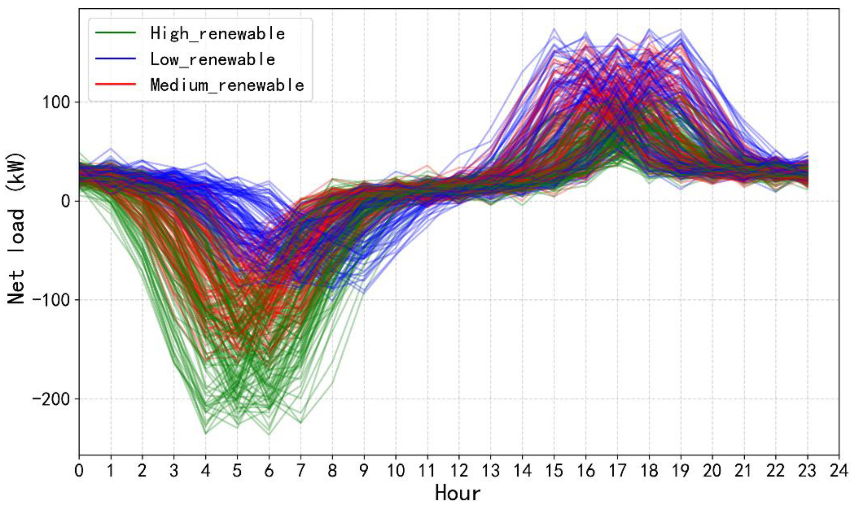
The optimization object of this study is a hybrid renewable energy system comprising photovoltaics (PV), wind power, local load, and a lithium-hydrogen hybrid energy storage system (HESS). The daily curves of PV output, wind output, and load are shown in Figs. (3)-(5). System optimization is conducted based on annual net-load data. To more intuitively present load characteristics and to select representative scenarios for validating the algorithm, the annual net-load profiles are clustered by renewable energy penetration into high, medium, and low scenarios, as shown in Figure 6. The main technical and economic parameters of the HESS are summarized in Table 1.
Figure 3.
The daily photovoltaic output curve.
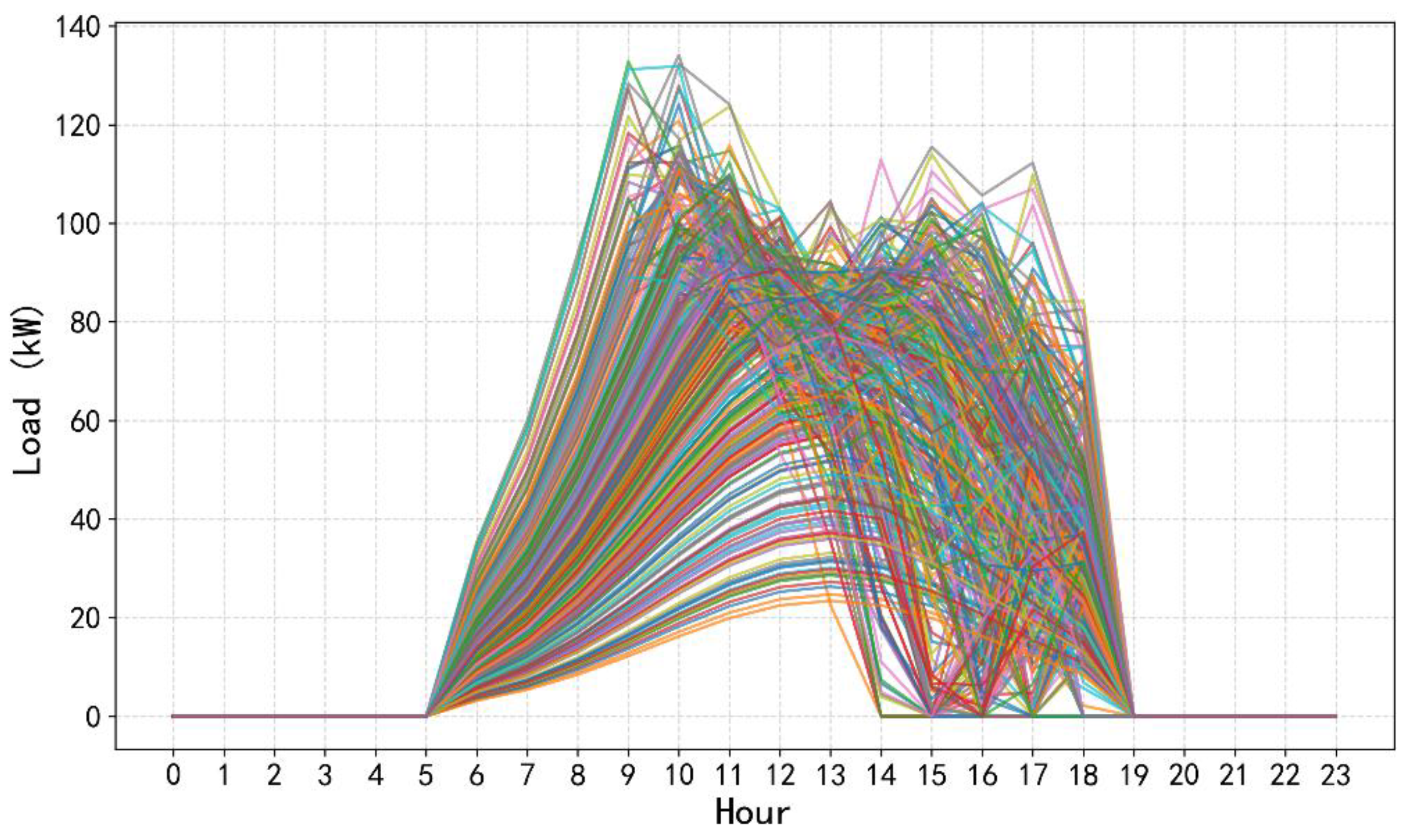
Figure 4.
The daily wind power output curve.
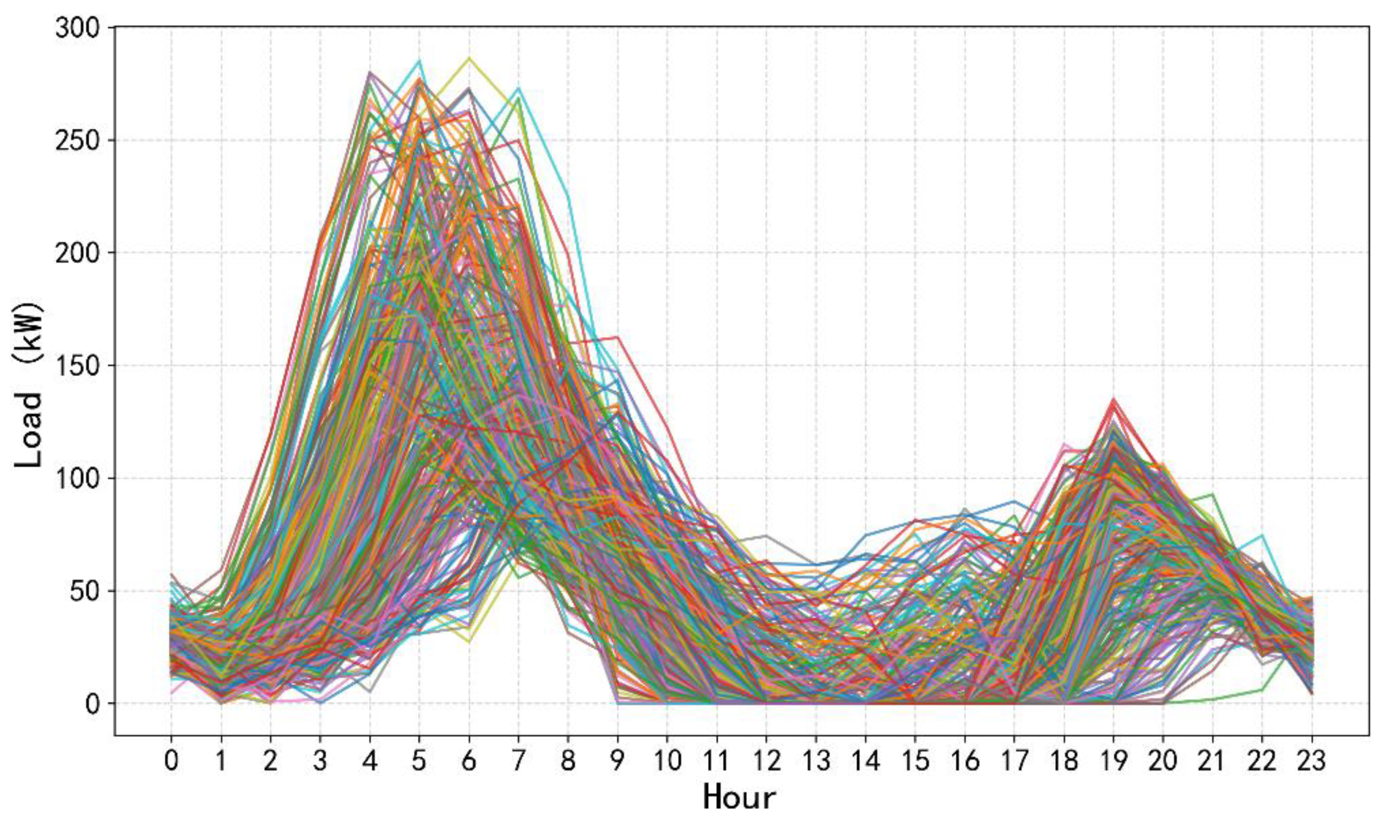
Figure 5.
The daily load curve.
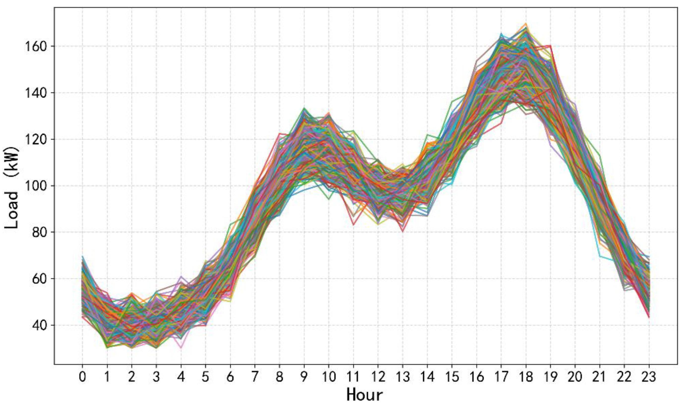
Figure 6.
The daily net load curve.
4.2. Algorithmic Solution and Results Analysis
The computing platform used for the solution is configured as follows: an Intel Core i9-14900K processor (24 cores, 32 threads), 128 GB RAM, and an NVIDIA RTX 4090 24 GB discrete GPU.
The training curves of the DRL-Gurobi cooperative algorithm are shown in Figure 7, indicating convergence. Using the proposed cooperative approach, the optimal HESS configuration is obtained. Using the proposed cooperative approach, the optimal HESS capacity configuration is obtained. As shown in Table 2, under the condition that the power deviation does not exceed 0.01, the minimum daily total cost is $209.10.
To further illustrate the internal operation mechanism of the system, Figure 8 presents the coordinated operation strategy of each HESS component under a representative net-load profile (high-penetration scenario).
Figure 8(a) illustrates the power profile over the typical day, capturing the dynamic relationships among the electrolyzer, fuel cell, battery charging/discharging, and net load. Figure 8(b) depicts the evolution of the battery state of charge (SoC) and the state of hydrogen storage tank (SoH).
At night (00:00-06:00 and 18:00-24:00), the net load remains negative. During these periods, the electrolyzer operates at a large scale, converting surplus electricity into hydrogen for storage; battery charging mainly occurs during the low-demand hours, cooperating with the electrolyzer to absorb excess energy.
During the daytime (09:00-12:00 and 15:00-18:00), the net load is markedly positive. The fuel cell and battery discharge jointly support power supply, performing peak shaving and valley filling. The battery SoC shows obvious charge-discharge cycles: charging in the early morning and at night, and rapid discharging during daytime load peaks. The SoC peaks at about 90% and falls to as low as 10%, indicating that the battery undertakes fast and deep regulation tasks.
The SoH exhibits relatively small variations with a gradual rise-fall pattern: it increases at night due to hydrogen production by the electrolyzer and declines during the day as the fuel cell consumes hydrogen for power generation. The changes are smooth, highlighting the long-cycle energy shifting characteristic of hydrogen storage. The battery and hydrogen storage are complementary across time scales: the battery primarily addresses short-term, rapid fluctuations, while hydrogen storage achieves inter-period energy balancing.
4.3. Comparative Analysis
To comprehensively validate the effectiveness of the proposed TD3-Gurobi cooperative optimization framework, three comparative cases are designed from different validation perspectives:
Case 1 (Proposed method): TD3-based deep reinforcement learning in the outer layer and the Gurobi mixed-integer programming solver in the inner layer.
Case 2 (Comparative algorithm verification): The outer layer uses the standard genetic algorithm (GA) and particle swarm optimization algorithm (PSO) combined with the inner layer Gurobi solver. And Gurobi is set to directly solve the two-level optimization problem for comparison. GA and PSO are selected to examine whether the proposed DRL method outperforms mature metaheuristics on high-dimensional continuous decision problems, in terms of solution quality (achieving lower cost) and convergence efficiency (shorter computation time). Although mathematical programming methods can theoretically obtain global optimal solutions, they often face the problem of excessively long solution times or even failure to converge. Therefore, a comparison with traditional deterministic algorithms (Gurobi solvers) aims to demonstrate whether the proposed algorithm can significantly improve computational efficiency while ensuring solution quality.
Case 3 (System architecture validation): Configure a single-storage system only (either battery storage or hydrogen storage) and solve it using the same optimization method as in Case 1. This comparison is designed to verify the advantages of the hybrid energy storage system over single-storage technologies in terms of economic performance and technical efficacy.
The performance of each scheme on key economic and technical indicators is summarized in Table 3.
The comparative analysis indicates substantial differences in economic performance and computational efficiency across optimization methods and storage configurations.
Case 1 (TD3 + Gurobi) achieves the most balanced performance, with a total cost of only $209.10 and a computation time of just 1.3 seconds.
In Case 2, the total costs of GA+G and PSO+G are 4.90% and 1.32% higher than Case 1, respectively, and their computation times are 250 s and 225 s, approximately 192× and 173× that of Case 1. This indicates that metaheuristic algorithms converge more slowly and have limited global search capability for complex optimization problems. Although the Gurobi approach attains the lowest total cost, its computation time is about 1385× that of Case 1, implying that while it can theoretically approach the global optimum, its efficiency is too low for complex, nonconvex, high-dimensional problems and thus fails to meet rapid decision-making requirements.
Case 3 further validates the structural advantages of the hybrid storage system. Although the battery storage scheme provides fast response, it requires an oversized capacity (3297.74 kWh) to satisfy energy balance, resulting in a total cost of $473.35, which is substantially higher than that of the hybrid system. The hydrogen energy storage solution has the lowest cost ($140.19), but its response rate cannot meet the system flexibility requirements. In contrast, the hybrid energy storage system achieves complementary capacity configuration between the battery and hydrogen storage, optimizes the balance of power and energy, and simultaneously delivers economy, flexibility, and operational stability.
4.4. Sensitivity Analysis
4.4.1. Sensitivity Analysis of Key Component Costs
To evaluate the robustness of the proposed method and identify the main cost drivers, this study conducted a sensitivity analysis on the costs of key components, including the electrolyzer power, fuel cell power, hydrogen tank, and the power and energy capacity of lithium battery. The corresponding optimal HESS configurations are shown in Table 4, Table 5, Table 6, Table 7 and Table 8, respectively. The details are as follows:
- (1)
- Sensitivity to Electrolyzer Power Cost
Variations in the electrolyzer power cost have a pronounced impact on system configuration and total cost. When the cost increases from 550 $/kW to 1021 $/kW, the average daily total cost rises from $186.71 to $231.62 (+24.0%). The hydrogen storage tank capacity decreases from 232.94 kg to 72.45 kg (-68.9%), indicating that the system mitigates higher electrolyzer costs by reducing hydrogen storage capacity. Correspondingly, the battery storage capacity increases from 158.19 kWh to 521.15 kWh (+229.4%), reflecting the substitution effect of battery storage for hydrogen storage. These results indicate that the electrolyzer cost is a key determinant of the economic performance of the hybrid storage system.
- (2)
- Sensitivity to Fuel Cell Power Cost
Changes in the fuel cell power cost have a relatively moderate impact on the system. When the cost increases from 200 $/kW to 371 $/kW, the average daily total cost rises only from $205.98 to $215.13 (+4.4%).
- (3)
- Sensitivity to Hydrogen Tank Cost
Changes in the hydrogen tank cost significantly affect the system’s configuration strategy. When the cost increases from 800 $/kg to 1486 $/kg, the average daily total cost rises from $187.76 to $219.14 (+16.7%). The hydrogen storage tank capacity decreases from 255.82 kg to 57.52 kg (-77.5%). To compensate for the reduction in hydrogen storage, the battery storage capacity increases from 120.08 kWh to 553.54 kWh (+361.0%), reflecting a cost-driven technology substitution effect and indicating that hydrogen tank cost is a key economic factor influencing long-term storage technology choices.
- (4)
- Sensitivity to Lithium Battery Power Cost
Variations in the lithium battery power cost have a relatively small effect on the total system cost. When the cost increases from 300 $/kW to 557 $/kW, the average daily total cost rises from $207.81 to $217.57 (+4.7%).
- (5)
- Sensitivity to Lithium Battery Energy-Capacity Cost
Changes in the lithium battery energy-capacity cost have a pronounced impact on system configuration. When the cost rises from 250 $/kWh to 464 $/kWh, the average daily total cost increases from $179.71 to $220.08 (+22.5%). When the capacity cost is relatively low (250 -321 $/kWh), the system substantially increases the battery energy capacity (up to 611.26 kWh) while reducing investment in hydrogen storage, reflecting a cost-driven technology substitution effect.
Ranked by the magnitude of total cost variation, the cost sensitivities of the components from highest to lowest are: electrolyzer power cost (24.0%) > lithium battery energy-capacity cost (22.5%) > hydrogen tank cost (16.7%) > lithium battery power cost (4.7%) > fuel cell power cost (4.4%).
The proposed algorithm enables robust configuration adjustments in response to changes in component costs, maintaining overall economic performance through a dynamic balance between battery storage and hydrogen storage. When the cost of one storage technology increases, the system automatically raises the configuration share of the other, demonstrating the technological complementarity of the hybrid energy storage system.
4.4.2. Sensitivity Analysis of Renewable Energy Penetration
Optimization is performed separately under the three typical renewable energy penetration scenarios: high, medium, and low. The optimal HESS configuration is shown in Table 9. The optimal operation results are shown in Figures 8, 9, and 10, respectively.
It can be observed that under the low-penetration scenario, renewable generation is insufficient; the required electrolyzer capacity is relatively small, but a higher-power fuel cell is needed to supplement electricity and ensure supply stability, while large hydrogen reserves are required to address long-term energy deficits. Under the medium-penetration scenario, the battery undertakes more short-term regulation tasks and the hydrogen demand is relatively low; under the medium-penetration scenario, the battery accounts for a higher share in short-term fluctuation mitigation, and both medium and low penetration scenarios require larger battery capacities to balance energy. In the low-penetration case, maintaining stable system operation also necessitates larger-capacity fuel cells and hydrogen storage, leading to a significant increase in cost.
Under the high-penetration scenario, the battery SoC exhibits a dual-peak charging pattern, reaching about 90% around 03:00-04:00 and 15:00. Discharging mainly coincides with the load peaks at 10:00-11:00 and 19:00-20:00, with the minimum SoC dropping to around 10%. Under medium penetration, the battery SoC can reach nearly 100% and remain there for an extended period, followed by rapid discharging during peak-load hours to about 25%. Under low penetration, the battery charges overnight to approximately 90% and then remains stable, with a gradual daytime discharge to a minimum of roughly 15%.
For the hydrogen storage tank, under high penetration, SoH slowly rises from about 50% to 65%, reflecting the smooth characteristics of long-duration storage. Under medium penetration, SoH quickly increases to around 100%, remains high for a considerable time, and then gradually declines, indicating higher utilization intensity. Under low penetration, SoH varies most gently, remaining essentially within the 45%-52% range, implying relatively low utilization.
The TD3-Gurobi cooperative optimization algorithm yields appropriate optimal configurations across all scenarios, demonstrating its robustness and adaptability. As renewable energy penetration increases, the importance of long-duration storage becomes more pronounced, while battery storage consistently provides indispensable fast regulation in all scenarios.
5. Conclusions
This paper proposes a bi-level cooperative optimization framework that integrates deep reinforcement learning (DRL) with mixed-integer programming (MIP) to jointly optimize the capacity configuration and operating strategy of a hybrid battery-hydrogen energy storage system. Targeting the minimization of average daily total cost and power deviation, the method achieves optimal capacity configuration and operation optimization of all system components. The results demonstrate that the proposed approach significantly outperforms conventional algorithms in both computational efficiency and solution quality, thereby verifying the advantages of hybrid storage over single-technology schemes. These findings demonstrate the feasibility and effectiveness of combining DRL with mathematical programming, providing a valuable reference for optimizing the configuration of complex energy systems.
The theoretical contribution lies in providing an efficient solution paradigm that fuses artificial intelligence with operations research for bi-level optimization problems characterized by strong coupling in energy systems. Future work may incorporate uncertainties in wind/PV and load forecasting, using stochastic programming or robust optimization to enhance reliability under complex conditions. In parallel, exploring diversified business models, such as the participation of storage in ancillary service markets, could further unlock the economic potential of hybrid energy storage systems.
Author Contributions
Conceptualization, T.Q.; methodology, T.Q.; software, T.Q.; validation, T.Q.; formal analysis, T.Q.; investigation, T.Q.; resources, T.Q.; data curation, T.Q.; writing—original draft preparation, T.Q.; writing—review and editing, T.Q.; visualization, T.Q.; supervision, K.Z.; project administration, T.Q.; funding acquisition, T.Q., L.Z. and D.S. All authors have read and agreed to the published version of the manuscript.
Funding
This research was funded by Jiangsu Provincial Science and Technology Project No. BK20230114, the Jiangsu Provincial Universities’ Basic Science Research General Project No. 23KJD470009, and the Talent-Introduction Research Start-up Fund No. 4170084.
Data Availability Statement
The raw data supporting the conclusions of this article will be made available by the authors on request.
Conflicts of Interest
The authors declare no conflicts of interest.
Abbreviations
The following abbreviations are used in this manuscript:
| HESS | Hybrid energy storage system |
| DRL | Deep reinforcement learning |
| EL | Electrolyzer |
| BESS | Battery energy storage system |
| MIP | Mixed integer programming |
| FC | Fuel cell |
| HST | Hydrogen storage tank |
| MDP | Markov Decision Process |
| TD3 | Twin Delayed Deep Deterministic Policy Gradient |
References
- Zhou, Z.; Ma, Z.; Mu, T. Hybrid energy storage capacity optimization based on VMD-SG and improved Firehawk optimization. Electr. Power Syst. Res. 2025, 239, 111218. [Google Scholar] [CrossRef]
- Lu, Q.; Yang, Y.; Chen, J.; Liu, Y.; Liu, N.; Cao, F. Capacity optimization of hybrid energy storage systems for offshore wind power volatility smoothing. Energy Rep. 2023, 9, 575–583. [Google Scholar] [CrossRef]
- Wu, X.; Shang, W.; Feng, G.; Huang, B.; Xiong, X. Coordinated control algorithm of hydrogen production-battery based hybrid energy storage system for suppressing fluctuation of PV power. Int. J. Hydrog. Energy 2024, 88, 931–944. [Google Scholar] [CrossRef]
- El-Ghazaly, M.; Abdel-Salam, M.; Nayel, M.; Hashem, M. Techno-economic utilization of hybrid optimized gravity-supercapacitor energy-storage system for enriching the stability of grid-connected renewable energy sources. J. Energy Storage 2025, 107, 115002. [Google Scholar] [CrossRef]
- Elkholy, M.; Schwarz, S.; Aziz, M. Advancing renewable energy: Strategic modeling and optimization of flywheel and hydrogen-based energy system. J. Energy Storage 2024, 101, 113771. [Google Scholar] [CrossRef]
- Hu, S.; et al. Model simulation and multi-objective capacity optimization of wind power coupled hybrid energy storage system. Energy 2025, 319, 134887. [Google Scholar] [CrossRef]
- Al-Quraan, A.; Athamnah, I. Economic tri-level control-based sizing and energy management optimization for efficiency maximization of stand-alone HRES. Energy Convers. Manag. 2024, 302, 118140. [Google Scholar] [CrossRef]
- Guven, A.F.; Abdelaziz, A.Y.; Samy, M.M.; Barakat, S. Optimizing energy dynamics: A comprehensive analysis of hybrid energy storage systems integrating battery banks and supercapacitors. Energy Convers. Manag. 2024, 312, 118560. [Google Scholar] [CrossRef]
- Li, B.; Wang, H.; Tan, Z. Capacity optimization of hybrid energy storage system for flexible islanded microgrid based on real-time price-based demand response. Int. J. Electr. Power Energy Syst. 2022, 136, 107581. [Google Scholar] [CrossRef]
- Wang, J.; Deng, H.; Qi, X. Cost-based site and capacity optimization of multi-energy storage system in the regional integrated energy networks. Energy 2022, 261, 125240. [Google Scholar] [CrossRef]
- Hu, Y.; et al. Optimal planning of electric-heating integrated energy system in low-carbon park with energy storage system. J. Energy Storage 2024, 99, 113327. [Google Scholar] [CrossRef]
- Rowe, K.; Mokryani, G.; Cooke, K.; Campean, F.; Chambers, T. Bi-level optimal sizing, siting and operation of utility-scale multi-energy storage system to reduce power losses with peer-to-peer trading in an electricity/heat/gas integrated network. J. Energy Storage 2024, 83, 110738. [Google Scholar] [CrossRef]
- Wang, Y.; et al. Research on planning optimization of integrated energy system based on the differential features of hybrid energy storage system. J. Energy Storage 2022, 55, 105368. [Google Scholar] [CrossRef]
- Li, X.; Li, M.; Habibi, M.; Najaafi, N.; Safarpour, H. Optimization of hybrid energy management system based on high-energy solid-state lithium batteries and reversible fuel cells. Energy 2023, 283, 128454. [Google Scholar] [CrossRef]
- Ye, Y.; Xu, B.; Wang, H.; Zhang, J.; Lawler, B.; Ayalew, B. Deep reinforcement learning-based energy management system enhancement using digital twin for electric vehicles. Energy 2024, 312, 133384. [Google Scholar] [CrossRef]
- Wu, Y.; et al. Integrated battery thermal and energy management for electric vehicles with hybrid energy storage system: A hierarchical approach. Energy Convers. Manag. 2024, 317, 118853. [Google Scholar] [CrossRef]
- Barelli, L.; Bidini, G.; Ciupageanu, D.A.; Pelosi, D. Integrating hybrid energy storage system on a wind generator to enhance grid safety and stability: A levelized cost of electricity analysis. J. Energy Storage 2021, 34, 102050. [Google Scholar] [CrossRef]
- Roy, P.; Liao, Y.; He, J. Economic dispatch for grid-connected wind power with battery-supercapacitor hybrid energy storage system. IEEE Trans. Ind. Appl. 2023, 59, 1118–1128. [Google Scholar] [CrossRef]
- Bharatee, A.; Ray, P.K.; Ghosh, A. A power management scheme for grid-connected PV integrated with hybrid energy storage system. J. Mod. Power Syst. Clean Energy 2022, 10, 954–963. [Google Scholar] [CrossRef]
- Wu, X.; Liu, L.; Wu, Y.; Luo, C.; Tang, Z.; Kerekes, T. Near-optimal energy management strategy for a grid-forming PV and hybrid energy storage system. IEEE Trans. Smart Grid 2025, 16, 1422–1433. [Google Scholar] [CrossRef]
- Dsouza, O.D.; Shilpa, G.; Rajnikanth; Irusapparajan, G. Optimized energy management for hybrid renewable energy sources with hybrid energy storage: An SMO-KNN approach. J. Energy Storage 2024, 96, 112152. [Google Scholar] [CrossRef]
- Sathishkumar, R.; Venkateswaran, M.; Deepamangai, P.; Rajan, P.S. An efficient power management control strategy for grid-independent hybrid renewable energy systems with hybrid energy storage: Hybrid approach. J. Energy Storage 2024, 96, 112685. [Google Scholar] [CrossRef]
- Adam, A.H.A.; Chen, J.; Kamel, S.; Safaraliev, M.; Matrenin, P. Power management and control of hybrid renewable energy systems with integrated diesel generators for remote areas. Int. J. Hydrog. Energy 2024, 89, 320–341. [Google Scholar] [CrossRef]
- Manandhar, U.; Zhang, X.; Beng, G.H.; Subramanian, L.; Lu, H.H.C.; Fernando, T. Enhanced energy management system for isolated microgrid with diesel generators, renewable generation, and energy storages. Appl. Energy 2023, 350, 121624. [Google Scholar] [CrossRef]
- Behera, P.K.; Pattnaik, M. Supervisory power management scheme of a laboratory scale wind-PV based LVDC microgrid integrated with hybrid energy storage system. IEEE Trans. Ind. Appl. 2024, 60, 4723–4735. [Google Scholar] [CrossRef]
- Ramu, S.K.; Vairavasundaram, I.; Palaniyappan, B.; Bragadeshwaran, A.; Aljafari, B. Enhanced energy management of DC microgrid: Artificial neural networks-driven hybrid energy storage system with integration of bidirectional DC-DC converter. J. Energy Storage 2024, 88, 111562. [Google Scholar] [CrossRef]
- Nkwanyana, T.B.; Siti, M.W.; Wang, Z.; Mulumba, W. Hybrid energy storage lifespan optimization based on an enhanced fuel-cell degradation model and meta-heuristic algorithm. Energy Rep. 2024, 12, 5712–5727. [Google Scholar] [CrossRef]
- Duong, H.-N.; Tran, L.; Vu, T.; Vo-Duy, T.; Nguyễn, B.-H. A global optimal benchmark for energy management of microgrid (GoBuG) integrating hybrid energy storage system. IEEE Trans. Smart Grid 2024, 15, 5429–5440. [Google Scholar] [CrossRef]
- Zhang, K.; Zou, G.; Zhang, J.; Li, H.; Sun, Y.; Li, G. Microgrid energy management strategy considering source-load forecast error. Int. J. Electr. Power Energy Syst. 2025, 164, 110372. [Google Scholar] [CrossRef]
- Tang, Y.; Xun, Q.; Liserre, M.; Yang, H. Energy management of electric-hydrogen hybrid energy storage systems in photovoltaic microgrids. Int. J. Hydrog. Energy 2024, 80, 1–10. [Google Scholar] [CrossRef]
- Sepehrzad, R.; Moridi, A.R.; Hassanzadeh, M.E.; Seifi, A.R. Intelligent energy management and multi-objective power distribution control in hybrid micro-grids based on the advanced fuzzy-PSO method. ISA Trans. 2021, 112, 199–213. [Google Scholar] [CrossRef]
- Chekira, O.; Boujoudar, Y.; El Moussaoui, H.; Boharb, A.; Lamhamdi, T.; El Markhi, H. An improved microgrid energy management system based on hybrid energy storage system using ANN NARMA-L2 controller. J. Energy Storage 2024, 98, 113096. [Google Scholar] [CrossRef]
- Wang, J.; Lyu, C.; Bai, Y.; Yang, K.; Song, Z.; Meng, J. Optimal scheduling strategy for hybrid energy storage systems of battery and flywheel combined multi-stress battery degradation model. J. Energy Storage 2024, 99, 113208. [Google Scholar] [CrossRef]
- Elkholy, M.H.; et al. A resilient and intelligent multi-objective energy management for a hydrogen-battery hybrid energy storage system based on MFO technique. Renew. Energy 2024, 222, 119768. [Google Scholar] [CrossRef]
- Intra-day and seasonal peak shaving oriented operation strategies for electric–hydrogen hybrid energy storage in isolated energy systems. Sustainability 2024.
- Han, F.; Zeng, J.; Lin, J.; Gao, C. Multi-stage distributionally robust optimization for hybrid energy storage in regional integrated energy system considering robustness and nonanticipativity. Energy 2023, 277, 127729. [Google Scholar] [CrossRef]
- Shan, J.; Lu, R. Multi-objective economic optimization scheduling of CCHP micro-grid based on improved bee colony algorithm considering the selection of hybrid energy storage system. Energy Rep. 2021, 7, 326–341. [Google Scholar] [CrossRef]
- Deng, J.; Wang, X.; Chen, T.; Meng, F. An energy router based on multi-hybrid energy storage system with energy coordinated management strategy in island operation mode. Renew. Energy 2023, 212, 274–284. [Google Scholar] [CrossRef]
- Pang, B.; Zhu, H.; Tong, Y.; Dong, Z. Optimal design and control of battery-ultracapacitor hybrid energy storage system for BEV operating at extreme temperatures. J. Energy Storage 2024, 101, 113963. [Google Scholar] [CrossRef]
- Mehraban, A.; Farjah, E.; Ghanbari, T.; Garbuio, L. Integrated optimal energy management and sizing of hybrid battery/flywheel energy storage for electric vehicles. IEEE Trans. Ind. Inf. 2023, 19, 10967–10976. [Google Scholar] [CrossRef]
- Li, M.; Wang, L.; Wang, Y.; Chen, Z. Sizing optimization and energy management strategy for hybrid energy storage system using multiobjective optimization and random forests. IEEE Trans. Power Electron. 2021, 36, 11421–11430. [Google Scholar] [CrossRef]
- Shen, X.; et al. Optimal hybrid energy storage system planning of community multi-energy system based on two-stage stochastic programming. IEEE Access 2021, 9, 61035–61047. [Google Scholar] [CrossRef]
- Xu, F.; Li, X.; Jin, C. Optimal capacity configuration and dynamic pricing strategy of a shared hybrid hydrogen energy storage system for integrated energy system alliance: A bi-level programming approach. Int. J. Hydrog. Energy 2024, 69, 331–346. [Google Scholar] [CrossRef]
- Gao, M.; Han, Z.; Zhang, C.; Li, P.; Wu, D.; Li, P. Optimal configuration for regional integrated energy systems with multi-element hybrid energy storage. Energy 2023, 277, 127672. [Google Scholar] [CrossRef]
- He, Y.; Guo, S.; Zhou, J.; Song, G.; Kurban, A.; Wang, H. The multi-stage framework for optimal sizing and operation of hybrid electrical-thermal energy storage system. Energy 2022, 245, 123248. [Google Scholar] [CrossRef]
- Li, C.; Zhang, X. Optimal sizing of hybrid energy storage system under multiple typical conditions of sources and loads. Int. J. Sustain. Energy 2025, 44, 2439298. [Google Scholar] [CrossRef]
- Atawi, I.E.; Abuelrub, A.; Al-Shetwi, A.Q.; Albalawi, O.H. Design of a wind-PV system integrated with a hybrid energy storage system considering economic and reliability assessment. J. Energy Storage 2024, 81, 110405. [Google Scholar] [CrossRef]
- Ganege, H.C.; Chandima, D.P.; Karunadasa, J.P.; Wheeler, P. Optimization of grid-connected solar PV systems with hybrid energy storage system: A case study of the Sri Lankan power system. J. Energy Storage 2025, 114, 115634. [Google Scholar] [CrossRef]
- Ma, Z.; Han, J.; Chen, H.; Houari, A.; Saim, A. Research on power allocation strategy and capacity configuration of hybrid energy storage system based on double-layer variational modal decomposition and energy entropy. J. Energy Storage 2024, 95, 112492. [Google Scholar] [CrossRef]
- Tsao, Y.-C.; Banyupramesta, I.G.A.; Lu, J.-C. Optimal operation and capacity sizing for a sustainable shared energy storage system with solar power and hydropower generator. J. Energy Storage 2025, 110, 115173. [Google Scholar] [CrossRef]
- Wang, G.; Blondeau, J. Optimal combination of daily and seasonal energy storage using battery and hydrogen production to increase the self-sufficiency of local energy communities. J. Energy Storage 2024, 92, 112206. [Google Scholar] [CrossRef]
- Yang, H.; Chu, Y.; Ma, Y.; Zhang, D. Operation strategy and optimization configuration of hybrid energy storage system for enhancing cycle life. J. Energy Storage 2024, 95, 112560. [Google Scholar] [CrossRef]
- Gomez-Gonzalez, M.; Hernandez, J.C.; Vidal, P.G.; Jurado, F. Novel optimization algorithm for the power and energy management and component sizing applied to hybrid storage-based photovoltaic household-prosumers for the provision of complementarity services. J. Power Sources 2021, 482, 228918. [Google Scholar] [CrossRef]
- Al-Quraan, A.; Athamnah, I.; Malkawi, A.M.A. Efficiency maximization of stand-alone HRES based on tri-level economic predictive technique. Sustainability 2024, 16, 10762. [Google Scholar] [CrossRef]
- Li, H.; et al. Collaborative optimization of VRB-PS hybrid energy storage system for large-scale wind power grid integration. Energy 2023, 265, 126292. [Google Scholar] [CrossRef]
- Liu, H.; Li, D.; Xiao, Z.; Qiu, Q.; Tao, X.; Qian, Q. Power Allocation and Capacity Optimization Configuration of Hybrid Energy Storage Systems in Microgrids Using RW-GWO-VMD. Energies 2025, 18, 4215. [Google Scholar] [CrossRef]
- Modu, B.; Abdullah, M.P.; Alkassem, A.; Hamza, M.F. Optimal rule-based energy management and sizing of a grid-connected renewable energy microgrid with hybrid storage using Levy flight algorithm. Energy Nexus 2024, 16, 100333. [Google Scholar] [CrossRef]
- Fujimoto, S.; van Hoof, H.; Meger, D. Addressing Function Approximation Error in Actor-Critic Methods. In Proceedings of the 35th International Conference on Machine Learning (ICML 2018), Stockholm, Sweden, 10–15 July 2018. [Google Scholar]
Figure 1.
Schematic diagram of a hybrid energy storage system.
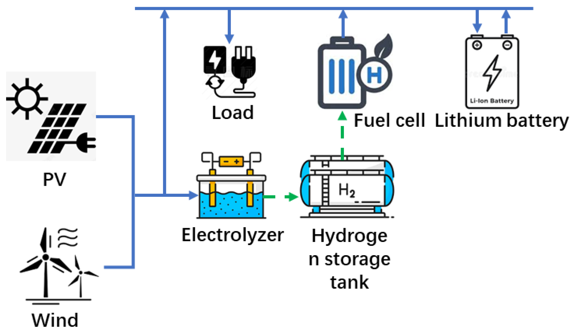
Figure 2.
Overall flowchart of the proposed algorithm.
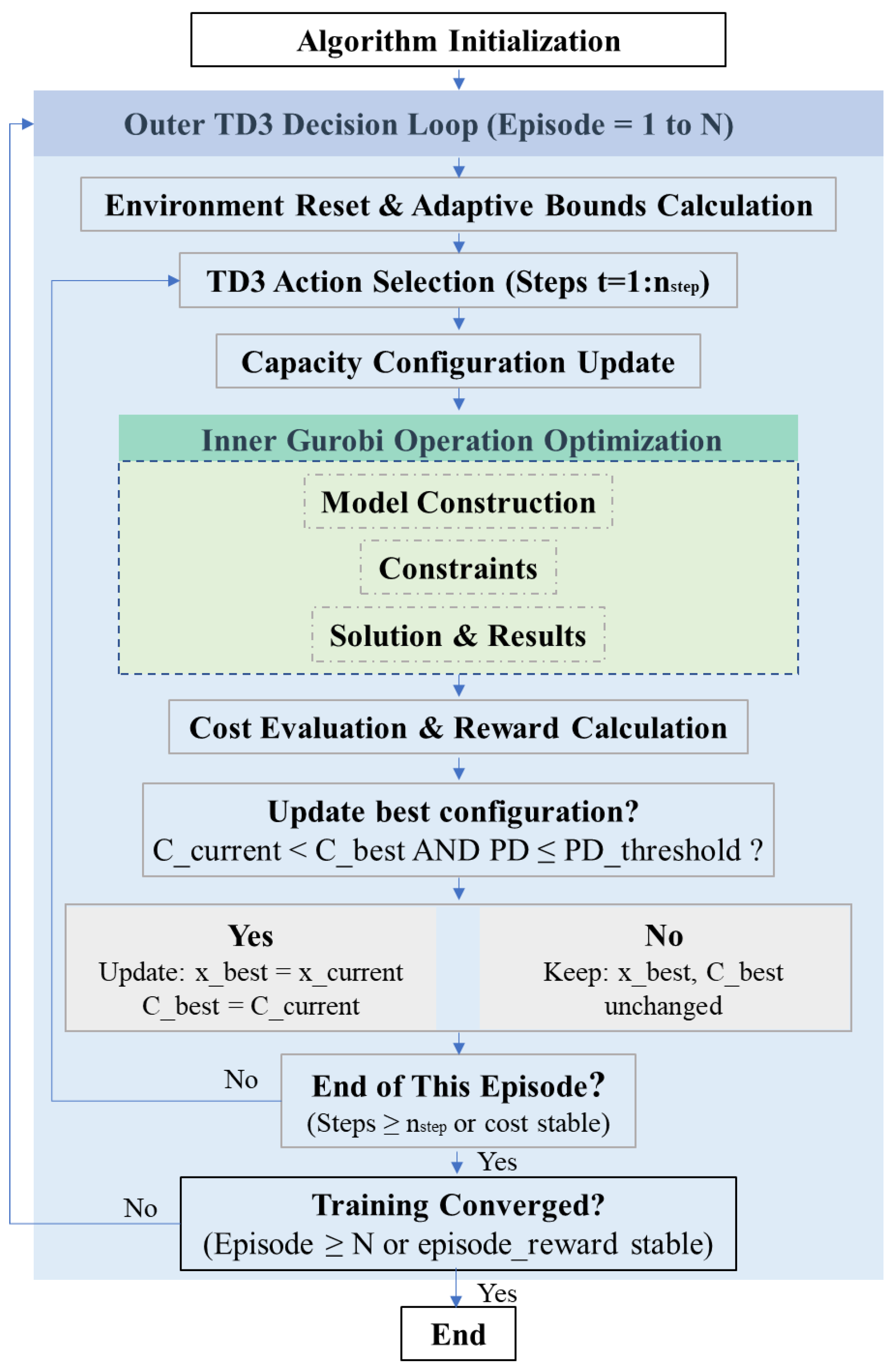
Figure 7.
The training curve of deep reinforcement learning in the proposed algorithm.

Figure 8.
The HESS coordinated operation strategy under typical high penetration conditions: (a) Power profile over the typical day; (b) Evolution of the battery state of charge (SoC) and the hydrogen storage tank state (SoH).
Figure 8.
The HESS coordinated operation strategy under typical high penetration conditions: (a) Power profile over the typical day; (b) Evolution of the battery state of charge (SoC) and the hydrogen storage tank state (SoH).
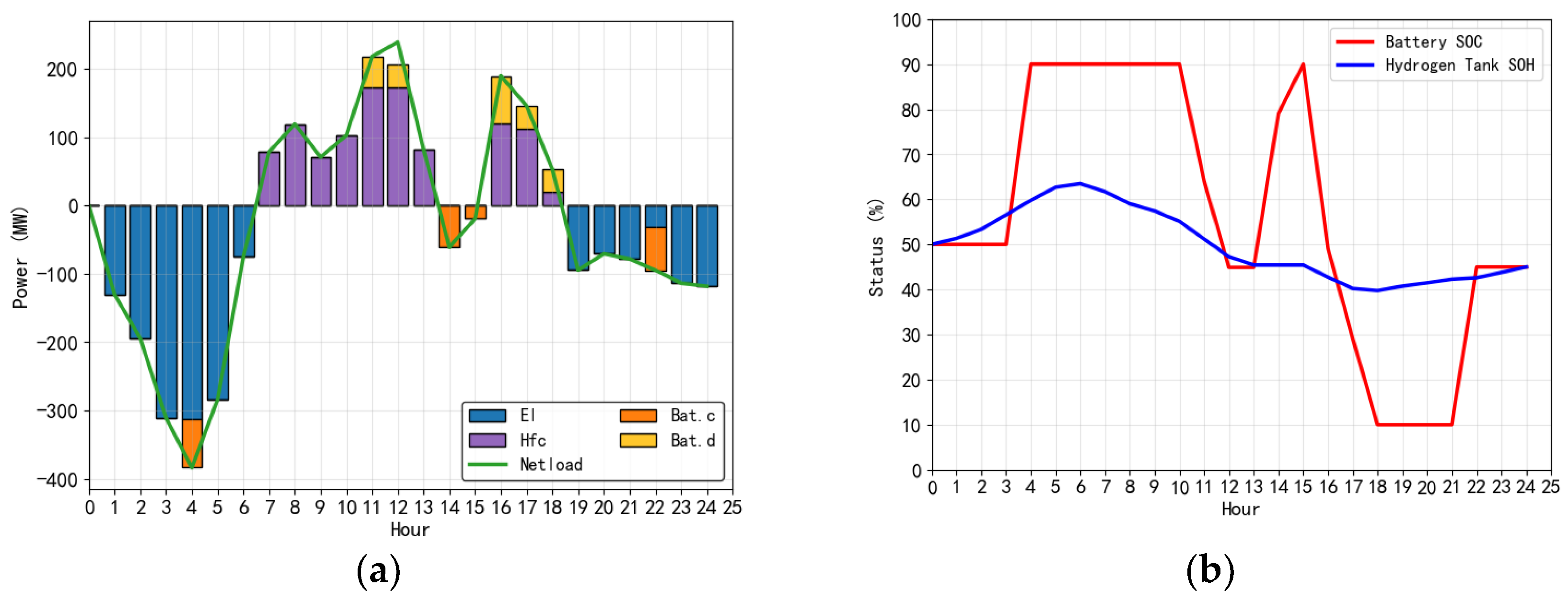
Figure 9.
The HESS coordinated operation strategy under typical medium penetration conditions: (a) Power profile over the typical day; (b) Evolution of the battery state of charge (SoC) and the hydrogen storage tank state (SoH).
Figure 9.
The HESS coordinated operation strategy under typical medium penetration conditions: (a) Power profile over the typical day; (b) Evolution of the battery state of charge (SoC) and the hydrogen storage tank state (SoH).
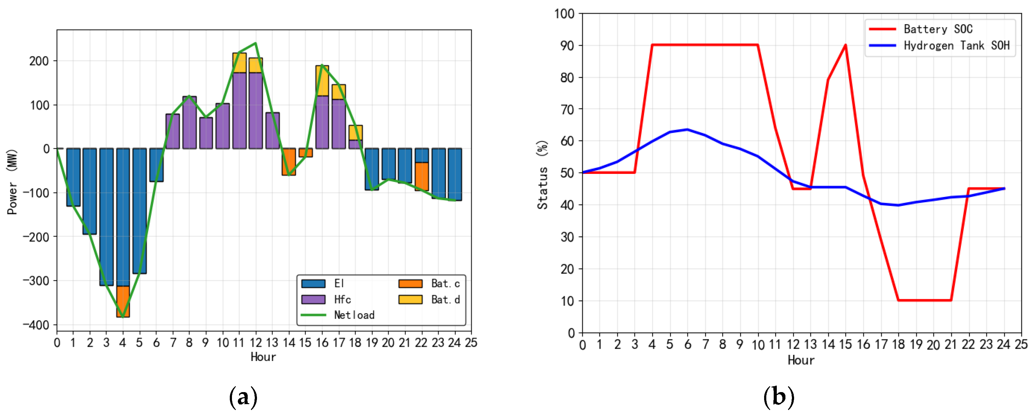
Figure 10.
The HESS coordinated operation strategy under typical low penetration conditions: (a) Power profile over the typical day; (b) Evolution of the battery state of charge (SoC) and the hydrogen storage tank state (SoH).
Figure 10.
The HESS coordinated operation strategy under typical low penetration conditions: (a) Power profile over the typical day; (b) Evolution of the battery state of charge (SoC) and the hydrogen storage tank state (SoH).
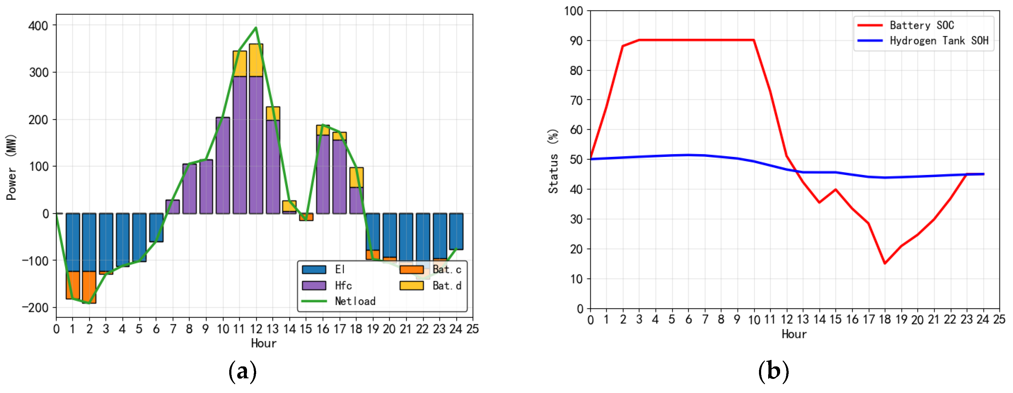

Table 1.
The main economic and technical parameters of the HESS.
| Component | Economic/Technical parameter | Value | Unit |
| EL (Electrolyzer) | 786 | $/kWh | |
| 0.8 | - | ||
| 0.4 | - | ||
| 70000 | Hour | ||
| HFC (Fuel Cell) | 286 | $/kW | |
| 0.6 | - | ||
| 0.3 | - | ||
| 30000 | Hour | ||
| HT (Hydrogen Tank) | 1143 | $/kg | |
| 0 | - | ||
| 1 | - | ||
| 0.97 | - | ||
| 0.98 | - | ||
| Battery | 429 | $/kW | |
| 357 | $/kWh | ||
| 0.98 | - | ||
| 0.98 | - | ||
| 0.1 | - | ||
| 0.9 | - | ||
| 10 | $/kWh | ||
| HESS(Hybrid Energy Storage System) | 20 | Year | |
| i | 0.08 | - | |
| Other | 33.33 | kWh/kg |
Table 2.
The optimal configuration results of HESS based on the proposed method.
| Decision variable | Optimized result | Unit |
| 312.23 | kW | |
| 173.26 | kW | |
| 225.90 | kg | |
| 71.60 | kW | |
| 174.68 | kWh | |
| Minimum daily total cost | 209.10 | $ |
Table 3.
Performance comparison of different optimization methods and energy storage configurations.
Table 3.
Performance comparison of different optimization methods and energy storage configurations.
| Cases | (kW) | (kW) | (kg) | (kW) | (kWh) | ($) | Computation time (s) | |
| Case 1 | DRL+G | 312.23 | 173.26 | 225.90 | 71.60 | 174.68 | 209.10 | 1.3 |
| Case 2 | GA+G | 262.88 | 93.19 | 112.77 | 133.42 | 460.72 | 219.34 | 250 |
| PSO+G | 279.96 | 115.35 | 146.30 | 104.32 | 353.56 | 211.87 | 225 | |
| G | 309.16 | 173.33 | 220.43 | 74.39 | 186.89 | 208.73 | 1800 | |
| Case 3 | Battery-only | - | - | - | 383.57 | 3297.74 | 473.35 | - |
| Hydrogen-only | 383.57 | 238.93 | 76.25 | - | - | 140.19 | - | |
Table 4.
The sensitivity analysis of electrolyzer power cost on HESS optimal configuration and minimum daily total cost.
Table 4.
The sensitivity analysis of electrolyzer power cost on HESS optimal configuration and minimum daily total cost.
| ($/kW) | (kW) | (kW) | (kg) | (kW) | (kWh) | ($) |
| 550 | 319.07 | 172.27 | 232.94 | 64.53 | 158.19 | 186.71 |
| 629 | 274.13 | 109.31 | 132.36 | 109.37 | 386 | 198.5 |
| 707 | 307.63 | 156.85 | 217.02 | 75.94 | 194.1 | 203.3 |
| 786 | 312.23 | 173.26 | 225.9 | 71.6 | 174.68 | 209.1 |
| 864 | 270.75 | 106.74 | 122.61 | 112.82 | 406.87 | 218.51 |
| 943 | 266.8 | 102.38 | 109.69 | 116.77 | 435.96 | 225.15 |
| 1021 | 255.13 | 93.96 | 72.45 | 128.44 | 521.15 | 231.62 |
Table 5.
The sensitivity analysis of fuel cell power cost on HESS optimal configuration and minimum daily total cost.
Table 5.
The sensitivity analysis of fuel cell power cost on HESS optimal configuration and minimum daily total cost.
| ($/kW) | (kW) | (kW) | (kg) | (kW) | (kWh) | ($) |
| 200 | 304.59 | 167.7 | 210.58 | 81.9 | 208.87 | 205.98 |
| 229 | 317.57 | 175.64 | 230.91 | 68.55 | 163.37 | 207.27 |
| 257 | 317.28 | 173.78 | 231.34 | 68.11 | 162.31 | 207.79 |
| 286 | 312.23 | 173.26 | 225.9 | 71.6 | 174.68 | 209.1 |
| 314 | 318.06 | 173.25 | 231.93 | 65.71 | 160.49 | 210.95 |
| 343 | 280.19 | 108.37 | 154.28 | 103.38 | 338.23 | 213.84 |
| 371 | 273.75 | 109.99 | 132.11 | 109.82 | 385.45 | 215.13 |
Table 6.
The sensitivity analysis of hydrogen storage tank cost on HESS optimal configuration and minimum daily total cost.
Table 6.
The sensitivity analysis of hydrogen storage tank cost on HESS optimal configuration and minimum daily total cost.
| ($/kg) | (kW) | (kW) | (kg) | (kW) | (kWh) | ($) |
| 800 | 334.53 | 181.63 | 255.82 | 49.54 | 120.08 | 187.76 |
| 914 | 320.07 | 175.68 | 234.14 | 63.54 | 155.56 | 194.59 |
| 1029 | 286.16 | 115.47 | 164.88 | 96.73 | 327.47 | 206.44 |
| 1143 | 312.23 | 173.26 | 225.9 | 71.6 | 174.68 | 209.1 |
| 1257 | 253.81 | 102.13 | 65.9 | 129.77 | 534.64 | 215.21 |
| 1371 | 251.5 | 90.13 | 59.94 | 132.91 | 548.25 | 216.69 |
| 1486 | 254.86 | 95.91 | 57.52 | 128.72 | 553.54 | 219.14 |
Table 7.
The sensitivity analysis of lithium battery power cost on HESS optimal configuration and minimum daily total cost.
Table 7.
The sensitivity analysis of lithium battery power cost on HESS optimal configuration and minimum daily total cost.
| ($/kW) | (kW) | (kW) | (kg) | (kW) | (kWh) | ($) |
| 300 | 305.77 | 169.31 | 212.97 | 80.29 | 203.19 | 207.81 |
| 343 | 306.89 | 171.54 | 215.44 | 77.49 | 197.67 | 208.86 |
| 386 | 306.34 | 171.57 | 215.45 | 78.51 | 199.52 | 209.82 |
| 429 | 312.23 | 173.26 | 225.9 | 71.6 | 174.68 | 209.1 |
| 471 | 273.55 | 125.53 | 131.58 | 110.09 | 386.62 | 213.42 |
| 514 | 314.97 | 180.85 | 259.79 | 57.69 | 143.77 | 216.62 |
| 557 | 278.22 | 146.66 | 131.77 | 107.87 | 386.84 | 217.57 |
Table 8.
The sensitivity analysis of lithium battery capacity cost on HESS optimal configuration and minimum daily total cost.
Table 8.
The sensitivity analysis of lithium battery capacity cost on HESS optimal configuration and minimum daily total cost.
| ($/kWh) | (kW) | (kW) | (kg) | (kW) | (kWh) | ($) |
| 250 | 249.66 | 88.36 | 53.83 | 134.04 | 561.86 | 179.71 |
| 286 | 244.15 | 99.73 | 53.04 | 146.54 | 611.26 | 198.23 |
| 321 | 264.4 | 99.8 | 101.19 | 119.17 | 455.11 | 203.01 |
| 357 | 312.23 | 173.26 | 225.9 | 71.6 | 174.68 | 209.1 |
| 393 | 285.23 | 150.21 | 168.27 | 98.33 | 304.06 | 217.79 |
| 429 | 311.65 | 168.48 | 225.19 | 77.5 | 177.39 | 218.42 |
| 464 | 325.33 | 174.73 | 241.01 | 58.71 | 142.63 | 220.08 |
Table 9.
The optimal HESS configuration and performance under different renewable energy.
|
Renewable energy penetration scenario |
(kW) | (kW) | (kg) | (kW) | (kWh) | ($) |
| High | 312.23 | 173.26 | 225.9 | 71.6 | 174.68 | 209.1 |
| Medium | 318.37 | 212.37 | 51.83 | 117.86 | 372.66 | 203.48 |
| Low | 123.18 | 290.64 | 1083.62 | 69.76 | 327.83 | 470.96 |
Disclaimer/Publisher’s Note: The statements, opinions and data contained in all publications are solely those of the individual author(s) and contributor(s) and not of MDPI and/or the editor(s). MDPI and/or the editor(s) disclaim responsibility for any injury to people or property resulting from any ideas, methods, instructions or products referred to in the content. |
© 2025 by the authors. Licensee MDPI, Basel, Switzerland. This article is an open access article distributed under the terms and conditions of the Creative Commons Attribution (CC BY) license (http://creativecommons.org/licenses/by/4.0/).
Copyright: This open access article is published under a Creative Commons CC BY 4.0 license, which permit the free download, distribution, and reuse, provided that the author and preprint are cited in any reuse.


