
Submitted:
01 October 2025
Posted:
02 October 2025
You are already at the latest version
Abstract
Quantum mechanics describes change as reversible and deterministic over unitary time, but we observe random change over nonunitary time. Thermocontextual mechanics (TCM) accommodates nonunitary time as fundamental by introducing two innovations. First, it defines states thermocontextually with respect to a measurement framework in equilibrium with the system’s actual surroundings, which always has a positive minimum temperature. This establishes ambient temperature, ambient heat, and exergy as objectively defined properties of state. Second, TCM’s “No hidden variables” law empirically defines states as measurable and definite. TCM’s second law is based on measurable changes in state before and after transitions between discrete measurable states. It codifies observations that a state only transitions in the direction of declining work potential on a fixed reference. It accommodates thermodynamics’ Second Law and statistical mechanics’ MaxEnt as distinct transition types. TCM’s third law codifies observations showing that networked transitions minimize irreversible losses. In the limit of reversibility, quantum processes are deterministic and unitary. By recognizing both unitary and nonunitary time, TCM explains previously unexplained observations strictly in terms of testable and empirically justified assumptions. These include the arrow of time, the measurement problem, nonlocality, and the spontaneous emergence of functional complexity.
Keywords:
time
; entropy
; quantum information
; foundations of physics
; emergence
; complexity
1. Introduction
Quantum mechanics formally defines the quantum state in terms of eigenfunctions of the Hamiltonian operator, which defines a system’s energy as the sum of kinetic and potential energy. A Hamiltonian eigenfunction defines a quantum eigenstate with a measurable and well-defined energy equal to the eigenvalue. The quantum state is geometrically expressed as a vector in a Hilbert space spanned by eigenvectors. The basis eigenvectors represent the measurable eigenstates for the Hilbert space’s reference framework. An isolated system has a fixed energy, and the eigenvectors are normalized to a fixed unit length.
A pure quantum state is represented by a single state vector spanning one or more basis eigenvectors. It completely specifies everything that can be known about a system’s state. If the state vector is an eigenvector, the state is a definite eigenstate measurable from the system’s measurement framework. If it is a vector sum of multiple eigenvectors, it is superposed, and from the Born rule [1], the probability of measuring a given eigenstate is equal to the square of the eigenfunction’s normalized amplitude.
A quantum state’s time change is given by Schrödinger’s equation:
is the quantum state at time t, is the Hamiltonian operator, and describes the state’s total energy as the sum of kinetic and potential energy. For an isolated system, energy is conserved, and the Schrödinger equation has the solution:
is a unitary operator, taking the state vector at time-zero to a new state vector at time t. Unitary time corresponds to a rotation of the state vector in Hilbert space. Unitary time is reversible and deterministic, and it preserves the initial state’s information.
If a system is prepared as an eigenstate, it has a definite observable state. Unitary time, however, can change it to a superposed state spanning multiple eigenvectors. If a system and its measurement device are isolated, then quantum mechanics describes the measurement as a reversible unitary process. Observation of the measurement result by an external observer, however, is necessarily an open-system process. Observation is generally irreversible and random, as described by thermodynamics’ Second Law [2] and statistical mechanics’ MaxEnt [3,4].
Quantum mechanics describes an isolated system’s evolution as strictly reversible and deterministic, but no system is perfectly isolated from its surroundings. A system plus its surroundings, by definition, is an isolated system, but we generally do not know the precise eigenstate of a system’s universe. If a system’s eigenstate is unknown, then the system can be described by a density matrix, ρ. The density matrix describes the system as a mixed state, and as an ensemble of eigenstate possibilities. An isolated system’s information is incomplete, but it is conserved. The density matrix’s time change is unitary, given by:
The density matrix’s unitary time change is given by the commutator of the density matrix and the Hamiltonian operator.
A non-isolated system of interest plus its surroundings defines an isolated system in which total information is conserved. The Lindblad equation describes the leakage of information from the density matrix for the system of interest to its surroundings [5]. This is a common and highly useful approach for describing open dissipative quantum systems. Its description of nonunitary time change, however, is based on an imperfect observer’s loss of information on the system of interest. Nonunitary time is a subjective and phenomenological description of irreversible and random change. Quantum mechanics’ Born-rule postulate can calculate the probabilities of random measurement results, but quantum mechanics cannot formally accommodate random change. The physical mechanism of wavefunction collapse, or whether it actually exists, is the quantum measurement problem.
Multiple quantum interpretations have been proposed to explain the randomness of quantum observations [6]. Eugene Wigner, who won the Nobel prize in 1963 for his work in quantum mechanics, concluded that an external observer’s consciousness triggers the random collapse of a superposed state to single observed state. The Many Worlds Interpretation asserts that at each random event, all possibilities, along with any observers, are instantiated in separate branches of an exponentially splitting universe. The De Broglie-Bohm interpretation asserts that the wavefunction is incomplete, and that random outcomes are deterministically dictated by hidden variables [7].
Determinism means that a state is connected to subsequent states by a linear chain of cause and effect. If we assume determinism, and if we further accept that the laws of physics apply to all systems, non-living and living, then we have superdeterminism [8]. Superdeterminism means that every action, and even every thought, was predetermined at the creation of time. All states and events across the universe are then deterministically correlated by common local connections in the primordial state. Superdeterminism can explain the determinism of unitary time, but it implies that all test results are predetermined, and therefore there can be no actual test of superdeterminism.
The interpretations described above are a few of the proposed explanations for reconciling the unitary time of quantum mechanics with the irreversibility and randomness of observations. They are all consistent with observations, but they are all based on untestable and unfalsifiable assumptions. Any explanation or theory that cannot be falsified is more properly described as speculative pseudoscience [9]. Quantum mechanics consequently focuses on verifiable experimental measurement results, and it avoids explanations or interpretations of empirical facts. This was the basis for David Mermin’s pithy “Shut up and calculate!” to summarize quantum mechanics’ standard Copenhagen interpretation [10]. Quantum mechanics provides unprecedently accuracy in its predictions, but its inability to provide testable explanations of irreversible and random observations underlines many open questions of physics. These include the measurement problem, instantaneous nonlocal correlations, and the emergence of complexity.
Whereas quantum mechanics describes nonunitary evolution of open systems as phenomenological, this paper takes a more fundamental approach. It addresses nonunitary time by objectively defining open systems’ states and their interactions from first principles. The paper is firmly based on the empirically validated assumptions of the thermocontextual interpretation (TCI) [11,12,13]. TCI was introduced as an alternative to the fundamental reversibility and determinism of Hamiltonian mechanics, which underlies modern classical, quantum, and relativistic mechanics. The paper expands upon and clarifies ideas in these earlier papers. It presents a strictly empirical framework for physics that recognizes irreversibility, randomness, and emergence as fundamental physical properties of nonunitary change.
2. Beyond the Hamiltonian State
A key step toward a fuller understanding of nonunitary time was taken in 2022, with Time and Causality: a thermocontextual perspective [11]. That article defined physical states thermocontextually with respect to a reference state in thermal equilibrium at the ambient temperature of the system’s surroundings. It resolved a system’s energy into thermocontextual energy components. Exergy is equal to the work potential on the system’s ambient surroundings, and entropic energy is equal to ambient heat, with zero capacity for work. It identified two distinct components of time. Unitary time describes a state’s reversible and deterministic changes. Nonunitary time describes the irreversible dissipation of exergy to entropic energy during transitions between states. Unitary and nonunitary time define the imaginary and real components of system time, a complex thermocontextual property of state. Subsequent articles described the self-organization of dissipative systems [12] and information and physical randomness [13]. TCI is more than just an interpretation of mechanics. It is reformulated here as thermocontextual mechanics (TCM), an empirically based and logically coherent framework for describing systems’ physical states and their irreversible and random transitions.
2.1. The TCM State
The thermocontextual state is based on the following assumptions:
- The Zeroth Law of thermodynamics. This establishes that temperature is a measurable property of state.
- The Third Law of thermodynamics. This establishes that absolute zero temperature cannot be reached in practice or in principle [14].
- No Hidden Variables of State. This asserts that a state is completely observable, in principle, by a perfect observer.
The first two assumptions are established laws of thermodynamics, and they are widely recognized as universally valid. They establish that a system’s surroundings have a positive temperature. The third postulate is an explicit declaration of empiricism and a rejection of untestable assumptions. The First Law of thermodynamics is not listed as an assumption of TCM because energy conservation is already firmly established as a physical fact. And significantly, TCM makes no presumption of determinism or reversibility, or for the irreversibility of thermodynamics’ Second Law.
The assumptions above provide the empirical foundation for the TCM state, illustrated in Figure 1. A system’s total energy (Et) is defined with respect to an inertial reference frame in the limit of absolute zero temperature. In addition to a reference frame, a system has physical surroundings at positive temperature(s). TCM defines the ambient temperature as the minimum positive temperature of the surroundings with which a system can potentially interact. The ambient temperature is the minimum temperature in a system’s universe and a thermocontextual property of state. It is the temperature of the ambient reference state (ARS) and the temperature of perfect measurement and observation.
The ARS is defined as spatially coincident with the system. The system and its ARS have kinetic and potential energies with respect to the inertial surroundings and external potential fields. The ARS also has thermal energy based on its positive ambient temperature. Figure 1 resolves a system’s total energy into the ARS energy and the system’s internal energy.
Internal energy U is defined relative to the ARS. It is resolved into heat and internal mechanical energy. Mechanical energy is the energy that remains after cooling to the ambient temperature, at which point the system has no thermal energy relative to the ARS. Internal mechanical energy includes kinetic energy from internal motions and potential energy from internally generated potential fields. Mechanical energy can be completely utilized for work on the ambient surroundings, and it is pure mechanical exergy, Xm.
Thermal energy is resolved into thermal exergy, Xq, and entropic energy, Q. Thermal exergy is the potential of a system’s thermal energy for work on the ARS by a reversible Carnot cycle. Thermal exergy is empirically defined by:
where Cv is the volumetric heat capacity, Tsys is the system’s temperature(s), and Ta is the temperature of the ambient surroundings. Entropic energy Q is the internal energy U minus exergy, with zero capacity for work. It is equivalent to thermal energy at the ambient temperature.
One final thermocontextual state property is thermal entropy. Thermal entropy is the ratio of entropic energy to the ambient temperature:
The last term shows that thermal entropy is a generalization of thermodynamics’ 3rd Law entropy, which is a special case with Ta=0.
TCM defines a system’s physical state with respect to the system’s actual surroundings at a positive, and generally changing, ambient temperature. A positive ambient reference temperature accommodates heat, exergy, and entropic energy as empirically measurable components of energy. The TCM state is objectively defined by measurements with respect to the ARS and by empirically justified assumptions. The Hamiltonian mechanical state, in contrast, is defined in the absence of thermal noise by hypothetical measurements at absolute zero temperature. Absolute-zero temperature measurements cannot reveal heat or thermal exergy; it can only record mechanical exergy. Absolute zero temperature, however, is unattainable. The Hamiltonian state is unmeasurable and based on a physically unjustified and untestable assumption.
2.2. States, Transitions, and System Time
The quantum wavefunction describes change as reversible and deterministic over unitary time. The outcomes of individual quantum measurements, however, are intrinsically random. Random measurement results are observable facts, but Hamiltonian and thermocontextual mechanics differ in their interpretations of measurement probabilities.
The determinism of Hamiltonian mechanics precludes defining measurement probabilities as a fundamental physical property. Probabilities are calculated by the Born-rule postulate [1]. Hamiltonian mechanics attributes random wavefunction collapse to unknown external perturbations of a physically superposed subsystem of interest. It describes measurement probabilities as Bayesian probabilities, based on an absolute-zero-temperature observer’s incomplete information and subjective expectations. Hamiltonian mechanics’ assumption of physically superposed states and wavefunction collapse due to unknown causes is consistent with observations, but consistency is not validation. A superposed wavefunction is a useful description of state, but a physically superposed state is intrinsically unobservable. The existence of physically superposed states is an untestable interpretation of empirical facts based on untestable assumptions.
TCM rejects assumptions that are not explicitly based on observations. This is formalized by TCM’s First Law:
First Law of TCM: There are no hidden variables of state.
No-hidden-variables means that states and state properties are perfectly and completely observable in principle [11,12,13]. It means that a state has surroundings from which a perfect ambient observer and measurement framework can completely describe it. The TCM state is definite and observable, whether it is observed or not. This does not imply, however, that a system is always observable or that it always exists as a state. The quantum Zeno effect, in fact, empirically establishes that a system’s state is not always observable [15].
The equally valid contrapositive of no-hidden-variables is that if a system’s state is not observable, then it does not exist as a state. TCM describes irreversible change as a sequence of discrete states and irreversible transitions between definite observable states, during which there is no state. Each transition irreversibly and discontinuously advances over nonunitary time.
Nonunitary transitions between discrete states are typically random. An initial definite state can transition to one of multiple possible states, each with its own transition probability. Transition probabilities are measurable frequentist probabilities [16]. Frequentist probabilities are experimentally defined, independent of an observer’s prior information, expectations, or assumptions. TCM regards transition probabilities as a measurable physical property of a system’s pre-transition state and a fixed measurement framework.
Between transitions, a system exists as an observable state. A time-dependent state can change over unitary time, but it exists within a single instant of irreversible nonunitary time, and its change is strictly reversible and deterministic. Unitary time is the imaginary component of system time, describing a system’s reversible and deterministic changes while it exists as a state [11].
Changes in system time are tracked by reference time, which marks the continuous “flow” of time as recorded by an external reference clock. It provides a continuous record of a system’s changes over reference time, whether that change is reversible, irreversible, or no change at all.
2.3. Microstates and Macrostates
A system’s microstate (eigenstate) completely describes a system’s physical state. The TCM microstate completely specifies both the system’s energy state and the configuration of its component parts. If a completely known microstate subsequently undergoes a random configurational transition, then the system’s post-transition configuration is incompletely known, and it is described as a macrostate. A macrostate (mixed quantum state) is an incomplete description of state defined by a statistical distribution of possible microstates:
is the probability that a measurement would reveal microstate , and N is the number of possible microstates. A macrostate’s measure of configurational incompleteness is given by its configurational entropy:
where is Boltzmann’s constant.
A microstate is defined with respect to its ARS, which changes with a system’s changing ambient surroundings. A macrostate, in contrast, is defined with respect to a fixed-information reference (FIR) at a fixed reference temperature, Tref. The transition probabilities in (6) and (7) are frequentist probabilities. They are empirically defined a perfect reference observer in equilibrium with the FIR.
The macrostate’s exergy is averaged over the individual microstates:
The in (8) are the same probabilities given in (7), and each is the corresponding microstate’s exergy. If a system is in thermal equilibrium, the probabilities are given by the Boltzmann-Gibbs distribution function as a function of the temperature and the microstate exergies [17]:
T is the equilibrium temperature of thermalization, and Z is a normalization factor for probabilities to sum to one. The function was defined in terms of the microscopic energy of a system’s particles, which corresponds to TCM exergy. A microstate with higher exergy has a lower probability of being measured. If all microstates have the same energy state, they are degenerate and equally probable, with =1/N. The macrostate’s configurational entropy is then maximized and equal to Boltzmann’s statistical entropy, :
The entropies described above are summarized in Table 1. For comparison, the table also shows the von Neumann entropy [18] for quantum systems, Shannon information entropy, which expresses uncertainties based on an observer’s Bayesian expectations [3,19], and Rudolf Clausius’s original definition of thermodynamic entropy.
TCM introduces accessible energy as a macrostate property to track a system’s changes. Accessible energy is defined by the capacity for work on the FIR. Like the microstate’s exergy, a macrostate’s accessible energy is resolvable into thermal and mechanical components:
Figure 2 resolves a microstate’s energy state into accessible and inaccessible energy components at time zero and at time t after irreversible dissipation, heat loss, and random transitions. The transition is assumed to be semi-isolated, during which the transition can only exchange ambient heat with the surroundings.
Thermal accessibility is the capacity of the system’s thermal exergy to do work on the FIR at the fixed reference temperature, . Thermal accessible energy is given by:
Thermal accessibility ranges from zero for , to a maximum of for . The macrostate’s thermalized energy, , (Figure 2) is inaccessible for work on the FIR. Thermal accessibility is independent of the ambient temperature for a semi-isolated transition, in which no work or exergy is exchanged with the surroundings.
The macrostate partitions the microstate’s mechanical exergy into mechanical accessibility, , and randomized mechanical energy, , (Figure 2). Mechanical accessibility is given by:
where is mechanical exergy that is randomized and not accessible for work on the FIR. The term inside the parentheses is an analogue to thermodynamics’ free energy: F = U – TS. Free energy is the empirically validated fraction of internal energy that is accessible for work on a reference at temperature T. is the internal mechanical accessibility and the fraction of internal mechanical exergy that is accessible for work at Tref.
3. Unitary and Nonunitary Transitions
3.1. Transitions and Nonunitary Time
TCM tracks a system’s microstate transitions by the changes in the system’s macrostate with respect to its fixed FIR. To track a microstate’s changes, we can set the macrostate and its FIR to the system’s microstate and ASR at time zero, as was illustrated in Figure 2. The macrostate completely describes the system’s initial energy state and microstate configuration.
Random changes in the system’s configuration subsequent to time zero lead to a loss of information and to an increase in the macrostate’s configurational entropy. From (12) and (13), increasing configurational entropy and dissipation by friction and irreversible heat flow lead to changes in the system’s microstate and macrostate. The changes between time zero and time t are illustrated in Figure 2.
The production of thermal entropy by irreversible dissipation of thermal or mechanical exergy is precisely the subject of the Second Law of thermodynamics. The production of configurational entropy by increasing randomness is precisely the subject of MaxEnt [3,19]. TCM generalizes both by introducing its Second Law (formerly Postulate Four [13]) to address the relative stability of states:
Second Law of TCM: (Stability of states—The Minimum Accessibility Principle): A transition that reduces a macrostate’s accessible energy is spontaneous, and it describes an irreversible transition from a less stable state to a more stable state.
Accessible energy is a macrostate property and a property of transitions. A state’s relative stability is based on a property of transitions, not on a property of state. TCM’s Second Law means that an isolated or semi-isolated system can only transition in the direction of declining accessible energy and increasing stability. A system’s accessible energy has a spontan0eous potential to decline until it reaches an equilibrium state of zero mechanical and thermal accessibility.
TCM’s Second Law is empirically vetted by the universally recognized successes of both MaxEnt and thermodynamics’ Second Law. However, whereas Hamiltonian mechanics regards these as phenomenological or emergent, TCM’s Second Law is firmly founded on empirically justified assumptions. It is an empirically defined and validated principle, and it is a fundamental law of physics. TCM’s Second Law establishes nonunitary time for transitions between definite states.
TCM recognizes two distinct types of nonunitary transitions leading to lower accessible energy: 1) energy-state transitions, and 2) random configurational instantiations. Production of thermal entropy by dissipation of thermal or mechanical exergy defines an energy-state transition. Production of configurational entropy by random configurational changes defines random instantiations. The transitions are described by a macrostate’s decline in accessible energy or by its production of configuration entropy. In both cases, changes are tracked across the macrostate’s continuously advancing reference time.
TCM describes energy-state transitions as random and spontaneous, without a triggering cause, internal or external. The decay of an unstable particle, for example, takes a high-exergy microstate to a definite lower-exergy microstate. Figure 3(A) shows the changes in a modified 2D Hilbert space spanned by the undecayed and decayed particles’ eigenstates. The modified Hilbert space in TCM is defined with respect to a reference framework for potential measurements at the positive ambient temperature of the system’s surroundings. The eigenvectors in 3(A) are normalized to the microstates’ different exergies. This contrasts with Hamiltonian mechanics, which represents eigenstates as normalized unit eigenvectors, reflecting a system’s fixed energy.
The unstable particle’s macrostate is a mixed state represented by the arc from the initial undecayed state toward the decayed state. The system is prepared at time zero as the undecayed state with probability of one, but the probability for the higher-stability decayed microstate continuously increases. At some point in time, the system randomly and spontaneously dissipates exergy and transitions to the more stable decayed state.
The macrostate deterministically predicts measurement probabilities at any point in time, but the energy-state transitions and measurement outcomes are intrinsically random. If an observation reveals the particle in its undecayed state, the macrostate is reset to the macrostate in 3(A) at time zero. If the particle is observed in its decayed state, the macrostate is reset to the definite time-invariant Decayed Microstate.
The other type of irreversible transition is random configurational instantiation. Configurational instantiation describes a state’s change in configuration, rather than energy state. Instantiation is triggered by an external interaction, such as a measurement. Figure 3(B) illustrates the random instantiation of an obliquely polarized photon by a polarized filter. At preparation, the photon is vertically polarized, and it has zero configurational entropy with respect to the FIR, set to the vertically polarized ARS.
Rotating the photon’s ARS to an oblique orientation changes the photon’s description from an eigenstate to a superposed state with statistical measurement outcomes represented by the dotted arrows. The photon is a superposition of virtual uninstantiated microstate potentialities with respect to the new ARS. It exists, however, as a definite and vertically polarized photon with respect to the FIR, and the macrostate has zero configurational entropy. Having a definite observable state makes the photon a pure state, regardless of the ASR or measurement framework.
After the photon encounters the obliquely polarized detector, the interaction randomly instantiates a photon with parallel or perpendicular polarization. The photon has a definite but unknown polarization (solid diagonal arrows). The macrostate is a superposition of vertically and horizontally polarized observables, and it has a positive configurational entropy. Finally, observation reveals the system’s new eigenstate. Information on the randomly instantiated photon resets the FIR and establishes a new zero-entropy macrostate equal to the now-known eigenstate.
3.2. Transition Stability and Unitary Processes
A transition takes an initial state to a final state. A sequence of transitions defines a process. A stationary process is sustained by component inputs from a stable source state, and after a series of transitions, it outputs waste components to the surroundings. It is observed that as a process is resolved into higher detail, it approaches a reversible quasistatic process. Hamiltonian mechanics, for example, describes friction as a sequence of reversible and deterministic steps dispersing macroscopic kinetic energy to the system’s particles.
While TCM’s Second Law establishes nonunitary transition as a fundamental fact, TCM’s Third Law explains why processes approach unitarity as closely as possible. TCM’s Third Law addresses the relative stability of irreversible transitions:
Third Law of TCM: (Stability of transitions—The Maximum Utilization Principle): A transition’s stability increases with higher energy utilization rates.
A transition’s utilization is the rate of accessible energy output as measured at the macrostate’s FIR. It is given by:
The equation shows that the rate of accessibility output is the sum of thermal and mechanical accessibility inputs, minus transition losses due to dissipation and randomization. The overdots designate derivatives over reference time, and is the mass transition rate. For notational simplicity, the overdot describes time-averaged rates for stationary processes and transitions. The overbars indicate specific properties, defined per unit mass.
TCM’s Third Law provides a transition with a drive to maximize its output of accessible energy. Equation (14) shows that accessible energy of input is conserved in the limit of a quasistatic process, in which the process is resolved into small reversible and deterministic increments. The Third Law drives processes to zero dissipation, zero randomization, and zero accessible energy loss.
In addition to minimizing accessible energy loss, the Third Law drives a transition to increase the accessibility of its input. Equations (4) and (12) show that thermal accessibility is maximized and equal to thermal exergy when the reference temperature and ambient temperatures are equal. Equality of reference and ambient temperatures also means that the macrostate is defined with respect to the microstate’s ASR. The macrostate then completely defines the microstate’s configuration, and this sets the macrostate’s configurational entropy to zero. From equation (13), this maximizes mechanical accessibility by setting it to mechanical exergy.
Zero dissipation means that there is no exergy loss. Zero increase in entropic entropy means no loss of mechanical accessibility. And equality of ambient and reference temperatures means maximizing accessible energy of input to equal the exergy input. Together, they establish reversibility, determinism, and unitarity of process. The unitarity of Hamiltonian mechanics is thus an idealized special case, based on extrapolation of TCM’s Third Law to zero dissipation, zero randomness, and complete information. Unitarity underlies Hamilton’s Least Action Principle [20], which is a fundamental principle of modern mechanics. Unitarity can be achieved and experimentally verified under highly controlled conditions. An example of unitary measurements of a nonlocal entangled system following a random transition is described next.
3.3. Nonlocal Unitary Measurements
One of the most perplexing facts of quantum mechanics is the experimental confirmation of instantaneous correlations of nonlocal measurements on entangled systems [21]. Instantaneous correlations do not allow faster-than-light communication, and they do not violate a strict interpretation of relativity. However, Hamiltonian mechanics cannot explain instantaneous correlations without assuming superdeterminism [8] or nonlocal hidden variables [7], neither of which is testable. TCM readily explains instantaneous nonlocal correlations across unitary time, based on its empirically testable assumptions.
Figure 4 shows a simple illustration of nonlocality, involving entangled photons. An entangled pair of photons is emitted from a source in opposite directions. When the photons encounter vertically polarized filters at time 2, they are randomly instantiated with definite vertical or horizontal polarization. Observations show that measurements conserve photon spin, with one vertically polarized and the other horizontally polarized, regardless of their separation.
We consider simultaneous measurements of the entangled photons using vertically polarized filters. Simultaneous measurements are made at points A0 and B0 in Figure 5. Conservation of quantum spin requires that measurements randomly instantiate a vertically polarized photon and a horizontally polarized photon. The instantaneous correlation of measurements at A0 and B0, outside of each other’s light cone (Figure 5), graphically illustrates nonlocality and Einstein’s “spooky action.”
When the photon interacts with Bob’s polarizer at point B0, it is randomly instantiated with vertical or horizontal polarization. Bob reversibly records and transmits the measurement result to Alice via a polarized signal photon with the orientation that he measured. Bob’s light cone and signal photon both reach Alice at A1. Based on Alice’s own results and her knowledge of the experimental protocol, she knows the orientation of Bob’s signal photon, and this allows her to reversibly measure it.
The reversibility and determinism of recording and transmitting measurement results creates a reversible and deterministic chain of causality. This is represented in Figure 5 by A0↔A1↔B0. The events occur within a nonlocal time-dependent microstate comprising the two detectors and the signal photon. The anticorrelated polarizations of the post-instantiation microstate conserves the zero spin of the entangled system’s source state.
There is no actual conflict between nonlocality and relativity. There is only an apparent conflict because we perceive the nonlocal microstate’s reversible changes from the perspective of a fixed-information reference’s irreversible reference time (right-hand axis). Alice does not see Bob’s result until her reference time tr,1, after measuring her own photon at reference time, tr,0. She perceives her observation of Bob’s signal photon at system time (ti,0,itu,1) as retroactively causing Bob’s anticorrelated detection at time (ti,0,itu,0). The time-dependent microstate, however, changes reversibly and deterministically over unitary time tu within a single instant of irreversible time, ti,0. There is no change in its information and no distinction between causality and retrocausality across reversible and deterministic unitary time.
3.4. Utilization-Rate Parameters
TCM’s Third Law states that transitions seek to increase their utilization. In this section, we consider how this happens. We can express a transition’s utilization rate as the sum of differential functions, one for each of its variables. Substituting equations (12) and (13) into (14), we get:
We consider a stationary process with a fixed source temperature and specific exergy, shown in bold. The variables in (15) are transition rate (), ambient temperature (), specific thermal entropy produced (), the increase in randomness (), and the randomized energy (). We can express the change in utilization rate as the sum of five differential functions, one for each of these variables:
Differentiating and inserting (15) into (16) yields the following set of differential equations:
Equations (17) to (21) show the changes in utilization of an individual transition in response to changes in mass transition rate, thermal and configurational entropy production rates, ambient temperature, and the randomized energy of input.
4. Emergence of Functional Complexity
A complex process is organized as a transition network [12]. Each node represents an elementary transition, which is objectively defined by the FIR’s resolution of accessible energy change measurements. Transition nodes are connected by component links which convey components from one transition node to another. A stationary transition network is sustained by input of high-accessibility components from a stable source and output of low-accessibility wastes to the environment.
Transition networks typically include exergonic [22] and endergonic [23] transition nodes, which exchange work via energy links. An exergonic transition takes a high-accessibility component and outputs a fraction of the component’s accessible energy decline as work on an endergonic node. An endergonic transition takes work from an exergonic node to pump a low-accessibility component to higher accessible energy. A transition’s utilization includes both the accessible energy of component outputs and the work by exergonic nodes on endergonic nodes within the network. A transition network’s overall utilization is given by the sum over the network’s elementary transitions:
The utilization of a complex process is a measure of the transition network’s functional complexity. The following sections describe various ways in which a sustained open system’s utilization and functional complexity can increase.
4.1. Maximize Growth (Maximize )
Open systems are commonly observed to expand into their environment. Fires spread, bacteria multiply, and their energy consumption rates increase. Equation (17) shows that a higher transition rate means a higher rate of utilization and higher stability. Given a source with fixed temperature and specific accessibility, a transition network can expand without limit. For real sources, however, the source’s state and environment are stressed at high transition rates, and growth is limited by the environment’s carrying capacity.
Increasing mass transition rate is a special-case response to TCM’s Third Law. Increasing the mass transition rate also increases the entropy production rate. This is commonly referred to as the Maximum Entropy Production Principle (MEPP) [24,25]. However, it is a special case and not a universal principle. Crecraft [12] showed that the spontaneous formation of a whirlpool falsifies the MEPP. As described next, increasing thermal entropy production by itself reduces efficiency, and it is destabilizing.
4.2. Maximize Efficiency (Minimize ):
A second path toward higher stability is by reducing thermal entropy production and maximizing efficiency. Equation (18) shows that decreasing the rate of thermal entropy production () increases utilization and stability. This is antithetical to the MEPP, which states that higher entropy production rate increases stability. The Second Law of thermodynamics mandates thermal entropy production, but equation (18) puts a brake on its increase. Reducing thermal entropy production increases the transition’s efficiency, output of accessible energy, and stability.
The spontaneous increase in a complex process’s utilization was documented in 1952 by Stanley Miller’s and Harold Urey’s ground-breaking experiment. They demonstrated the abiogenic synthesis of amino acids from a mixture of simple gases and water. They stimulated the gas mixture with a continuous electrical spark to simulate lightning in earth’s early atmosphere [26]. When they analyzed the system afterward, they found that the gas molecules had reorganized themselves into a variety of amino acids.
The production of low-entropy amino acids from a high-entropy gas mixture occurs with an input of exergy. Energy is conserved and entropy is produced by the dissipation of electrical exergy to heat. The experiment is consistent with the laws of thermodynamics and Hamiltonian mechanics, but consistency is not an explanation. Of the vast number of degenerate microstates compatible with the experiment’s initial macrostate, only a vanishingly small number could lead to the deterministic assembly of amino acids. The repeatability of the experiment within the Hamiltonian mechanical framework would require a spontaneous and unexplained finetuning of each and every experiment’s initial microstate to this vanishingly small subset of suitable microstates.
TCM’s Third Law provides a simple and direct explanation of the experimental results, without the need for finetuning. The continuous application of exergy and non-linear chemical kinetics maintain instability and transitions with multiple microstate potentialities. At each transition, the Third Law preferentially selects paths that reduce dissipation and increase accessible energy of the system. Sequential application of the Third Law over a vast number of incremental transitions guides the process to form a variety of high-energy amino acids from the gas mixture’s chemical components [12].
4.3. Thermal Refinement (Minimize )
A transition or process can also increase its stability by thermal refinement. Equations (15) and (19) show that reducing the ambient temperature is another means of reducing dissipation and increasing the mechanical accessibility of output. Thermal refinement thereby increases the transition’s stability. Thermal refinement is consequence of a declining ambient temperature, but its increase in utilization is measured with respect to the macrostate’s FIR at a fixed reference temperature.
If we take the cosmic microwave background temperature (TCMB) as the ambient temperature of the universe, then the cosmic microwave energy is ambient energy with zero accessibility. Rewriting equation (19) for an isolated system, the production of accessible energy due to cosmic expansion and cooling is given by A declining TCMB results in an increase in accessible energy. According to TCM’s Third Law, cosmic expansion and a cooling ambient temperature is more stable than a static or collapsing universe. In addition, a positive feedback between cosmic expansion and production of accessible energy might explain the acceleration of cosmic expansion, which is observed but unexplained [27,28].
4.4. Minimize Randomness (Minimize )
Equation (20) shows that reducing a transition’s randomness and its increase in configurational entropy increases its accessible energy output and stability. Minimizing a transition’s randomness provides a counterbalance to MaxEnt. MaxEnt says that a system’s configurational entropy spontaneously increases, but equation (20) puts a brake on its increase. Reducing the rate of randomization increases the rate of accessible energy output and transition stability.
The use of templates to create high-accessibility information-bearing nucleotides is well recognized as a key step in the abiogenic origin of life [29,30]. The stability of self-replicating templates, however, has previously been unexplained. Templates reduce the randomness of creating nucleotides, and they increase the process’s utilization and stability [13]. The stability of templates in the production of nucleotides is a predicted consequence of TCM’s Third Law [13].
4.5. Source Refinement (Minimize )
Another way to increase the accessible energy of output is to reduce the energy source’s randomized energy (21). This describes source refinement, which was introduced by Robert Griffiths in his Consistent Histories Interpretation of quantum mechanics [31]. Refinement is the acquisition of additional information by new measurements. The Third Law provides an open system with a drive to reset its macrostate reference temperature to a lower ambient temperature and to acquire all accessible information on its energy source. This decreases the randomized energy of the transition’s input, and it increases the transition’s accessible energy output and stability.
An example of source refinement is a virus’s evolution [13]. Source refinement by a virus encodes information about its target host in the virus’s RNA. The acquired information enables the virus to increase its access and utilization of its host’s energy for reproduction, thereby increasing the virus’s fitness and stability. The drive for source refinement and reduction in configurational entropy corresponds to the proposed Second Law of information entropy [32].
5. Summary
Thermocontextual mechanics is a strictly empirical framework for physics that accommodates irreversibility and randomness as physical properties of state transitions. TCM generalizes Hamiltonian mechanics, which underlies modern physics. It defines a system’s state thermocontextually, with respect to a reference state at a positive ambient temperature. This adds ambient temperature, exergy (work capacity on the ambient reference), thermal entropy, and entropic energy (ambient heat) as thermocontextual properties of state. These are all measurable and objectively defined properties of state.
TCM proposes three new laws based on empirically measured facts and empirically justified assumptions. Its First Law, “no hidden state variables,” is an affirmation of TCM’s empiricism. It defines a system’s physical state by perfect measurement, and it establishes states as observable and definite. States can be time-dependent, but state changes are strictly reversible and deterministic. Not all change is reversible and deterministic, however. A system can reversibly and randomly transition between definite states, during which the system does not exist as a state. TCM’s Second and Third Laws describe the stability of states and transitions.
TCM’s Second Law states that a system can spontaneously transition only to states of lower accessible energy, which is the work capacity on a fixed reference state. TCM’s Second Law accommodates both the Second Law of thermodynamics and its statistical mechanical analogue, MaxEnt, as distinct special cases.
The Second Law of thermodynamics describes the spontaneous production of thermal entropy and the dissipation of exergy. Exergy is a system’s work potential on its ambient surroundings, which is not generally fixed. Dissipation of exergy defines an energy-state transition, such as the spontaneous decay of an unstable particle to a more stable state of lower exergy.
MaxEnt, in contrast, describes randomization and the increase in configurational entropy. This is illustrated by the measurement of a pure superposed state. Interaction of a pure superposed state with a measurement device randomly instantiates one of its measurable microstate potentialities. Prior to interaction, the pure state has a definite pre-transition microstate configuration. A pure superposed state is a superposition of measurable potentialities thermocontextually defined by a change in the system’s surroundings. Interaction of the system with its changed surroundings randomly instantiates one of its microstate potentialities. Random instantiation increases the uncertainty and configurational entropy with respect to the system’s fixed-information FIR (prior to observation).
TCM’s Second Law formally establishes an arrow of time for states. It is defined in terms of first principles and empirically justified assumptions. The universal experimental validation of thermodynamics’ Second Law [2] and MaxEnt [3,4] establishes TCM’s Second Law as a fundamental principle of physics.
TCM’s Third Law addresses the stability of transitions and transition networks. It states that the stability of a transition increases with its output of accessible energy. In the limit of maximum stability, there is no loss of work potential by dissipation or randomization. The absence of dissipation and randomness defines a reversible unitary process. The unitarity of quantum processes and the Least Action Principle are special cases of TCM’s Third Law, applicable in the limit of perfectly reversible utilization of energy.
For less-than-perfect utilization, the Third Law makes specific predictions about functionally complex transition networks that Hamiltonian mechanics can only describe as emergent. The Third Law successfully predicts the spontaneous emergence of complex high-energy amino acids in the Miller-Urey experiment. It provides a selection principle for a transition network to maximize transitions’ accessible energy output to other transitions within the network. This guides the network to spontaneously increase its accessible energy and to self-organize functionally complex processes. Spontaneous self-organization and increasing functional complexity is experimentally well documented for far-from-equilibrium systems [33]. TCM’s Third Law is based on empirically justifiable assumptions. It is an empirically defined and tested description of non-equilibrium systems, and it is a fundamental principle of physics.
By defining states with respect to a positive-temperature reference state, TCM expands the scope of Hamiltonian mechanics from a description of static unitary states to a description of states and their nonunitary transitions. TCM provides a fresh perspective on many long-standing problems of physics, including the measurement problem, nonlocality, and the emergence of functional complexity. It represents a major reformulation of physics, accommodating mechanics, thermodynamics, and the emergence of complexity, all within a single framework of physics.
Funding
This research received no external funding.
Data Availability Statement
No new data were created or analyzed in this study
Conflicts of Interest
The author declares no conflicts of interest.
Abbreviations
The following abbreviations are used in this manuscript:
| TCM | Thermocontextual Mechanics |
| ASR | State’s ambient reference state |
| FIR | Macrostate’s fixed-information reference |
References
- Born Rule. Wikipedia, Wikimedia Foundation. Available online: https://en.wikipedia.org/wiki/Born_Rule (accessed on 27 September, 2025).
- Lieb, E.; Yngvason, J. The physics and mathematics of the second law of thermodynamics. Physics Reports 1999, 310, 1–96. [Google Scholar] [CrossRef]
- Jaynes, E.T. Information theory and statistical mechanics. Physical review 1957, 106. [Google Scholar] [CrossRef]
- Dias, T.C.M.; Diniz, M.A.; Pereira, C. A. d. B.; Polpo, A. Overview of the 37th MaxEnt, Entropy 2018, 20. [CrossRef]
- Manzano, D. Manzano, D. A short introduction to the Lindblad master equation. AIP advances 2020, 10. [CrossRef]
- Interpretations of quantum mechanics. Wikipedia, Wikimedia Foundation. Available online: https://en.wikipedia.org/wiki/Interpretations_of_quantum_mechanics. (accessed on 5 September 2025).
- Goldstein, S. Bohmian Mechanics. In The Stanford Encyclopedia of Philosophy, Summer 2024 Edition. Zalta, E.; Nodelman, U.; Eds; https://plato.stanford.edu/archives/sum2024/entries/qm-bohm/.
- Superdeterminism. Wikipedia, Wikimedia Foundation. Available online: https://en.wikipedia.org/wiki/Superdeterminism (accessed on 15 May, 2025).
- Karl Popper. Wikipedia, Wikimedia Foundation. Available online: https://en.wikipedia.org/wiki/Karl_Popper (accessed on September, 2025).
- Mermin, N.D. Could Feynman Have Said This? Physics Today. 2004, 57, 10–11. [Google Scholar] [CrossRef]
- Crecraft, H. Time and Causality: A Thermocontextual Perspective, Entropy 2022, 23.12. [CrossRef]
- Crecraft, H Dissipation+ Utilization= Self-Organization, Entropy 2023, 25. [CrossRef]
- Crecraft, H. The Second Law of Infodynamics: A Thermocontextual Reformulation. Entropy 2025, 27. [Google Scholar] [CrossRef] [PubMed]
- Masanes, L.; Oppenheim, J. A general derivation and quantification of the third law of thermodynamics, Nature communications 2017, 8. [CrossRef]
- Misra, B.; Sudarshan, B, E. The Zeno’s paradox in quantum theory. J. Math. Phys. 1977, 18, 756–763. [Google Scholar] [CrossRef]
- Frequentist probability. Wikipedia, Wikimedia Foundation. Available online: https://en.wikipedia.org/wiki/Frequentist_probability. (accessed on 10 August 2025).
- Boltzmann Distribution. Wikipedia, Wikimedia Foundation. Available online: https://en.wikipedia.org/wiki/Boltzmann_distribution. (accessed on 25 June 2025).
- Von Neumann Entropy. Wikipedia, Wikimedia Foundation. Available online: https://en.wikipedia.org/wiki/Von_Neumann_entropy (accessed on 16 February 2025).
- Bayesian statistics. Wikipedia, Wikimedia Foundation. Available online: https://en.wikipedia.org/wiki/Bayesian_statistics. (accessed on 16 April 2025).
- The Principle of Least Action Chapter 19: The Feynman lectures on physics. Vol 2, CalTech. Available online: https://www.feynmanlectures.caltech.edu/II_19.html (accessed on 1 July 2025).
- Freedman, S.; Clauser, J. Experimental test of local hidden-variable theories. Physical review letters 1972, 28. [Google Scholar] [CrossRef]
- Exergonic Reaction. Wikipedia, Wikimedia Foundation. Available online: https://en.wikipedia.org/wiki/Exergonic_reaction. (accessed on 11 September 2025).
- Endergonic Reaction. Wikipedia, Wikimedia Foundation. Available online: https://en.wikipedia.org/wiki/Endergonic_reaction. (accessed on 3 July 2025).
- Swenson, R. A grand unified theory for the unification of physics, life, information and cognition (mind). Philosophical Transactions of the Royal Society A 2023, 381. [Google Scholar] [CrossRef] [PubMed]
- Martyushev, L.M. Maximum entropy production principle: History and current status. Physics-Uspekhi 2021, 64. [Google Scholar] [CrossRef]
- Miller, S.L. Production of Amino Acids Under Possible Primitive Earth Conditions. Science 1953, 117, 528–9. [Google Scholar] [CrossRef] [PubMed]
- Lambda-CDM model. Wikipedia, Wikimedia Foundation. Available online: https://en.wikipedia.org/wiki/Lambda-CDM_model. (accessed on 3 July 2025).
- Cosmological constant problem. Wikipedia, Wikimedia Foundation. Available online: https://en.wikipedia.org/wiki/Cosmological_constant_problem (accessed on 3 July 2025).
- von Kiedrowski, G. Minimal replicator theory I: Parabolic versus exponential growth. In Bioorganic chemistry frontiers, Dugas, H., Schmidtchen, F. P. Eds.; Springer, New York, 1993; Volume 3, pp 113–146. [CrossRef]
- Szilágyi, A.; Zachar, I.; Scheuring, I.; Kun, Á.; Könnyű, B.; Czárán, T. Ecology and evolution in the RNA world dynamics and stability of prebiotic replicator systems. Life 2017, 7. [Google Scholar] [CrossRef] [PubMed]
- Griffiths, R. The Consistent Histories Approach to Quantum Mechanics. In The Stanford Encyclopedia of Philosophy Summer 2024 Edition; Zalta, E., Nodelman U., Eds.; https://plato.stanford.edu/archives/sum2024/entries/qm-consistent-histories/.
- Vopson, M.; Lepadatu, S. Second law of information dynamics. AIP Advances 2022, 12. [Google Scholar] [CrossRef]
- Nicolis, G.; Prigogine, I. Self-Organization in Nonequilibrium Systems: From Dissipative Structures to Order through Fluctuations Wiley Interscience, New York. 1977.
Figure 1.
Total energy and internal energy-state components. A system’s total energy is kinetic and potential energy (KE+PE) with respect to an inertial reference frame and external potential fields at absolute zero temperature. The internal energy state is defined with respect to a spatially-coincident ambient reference state (ARS) at a positive ambient temperature, Ta.
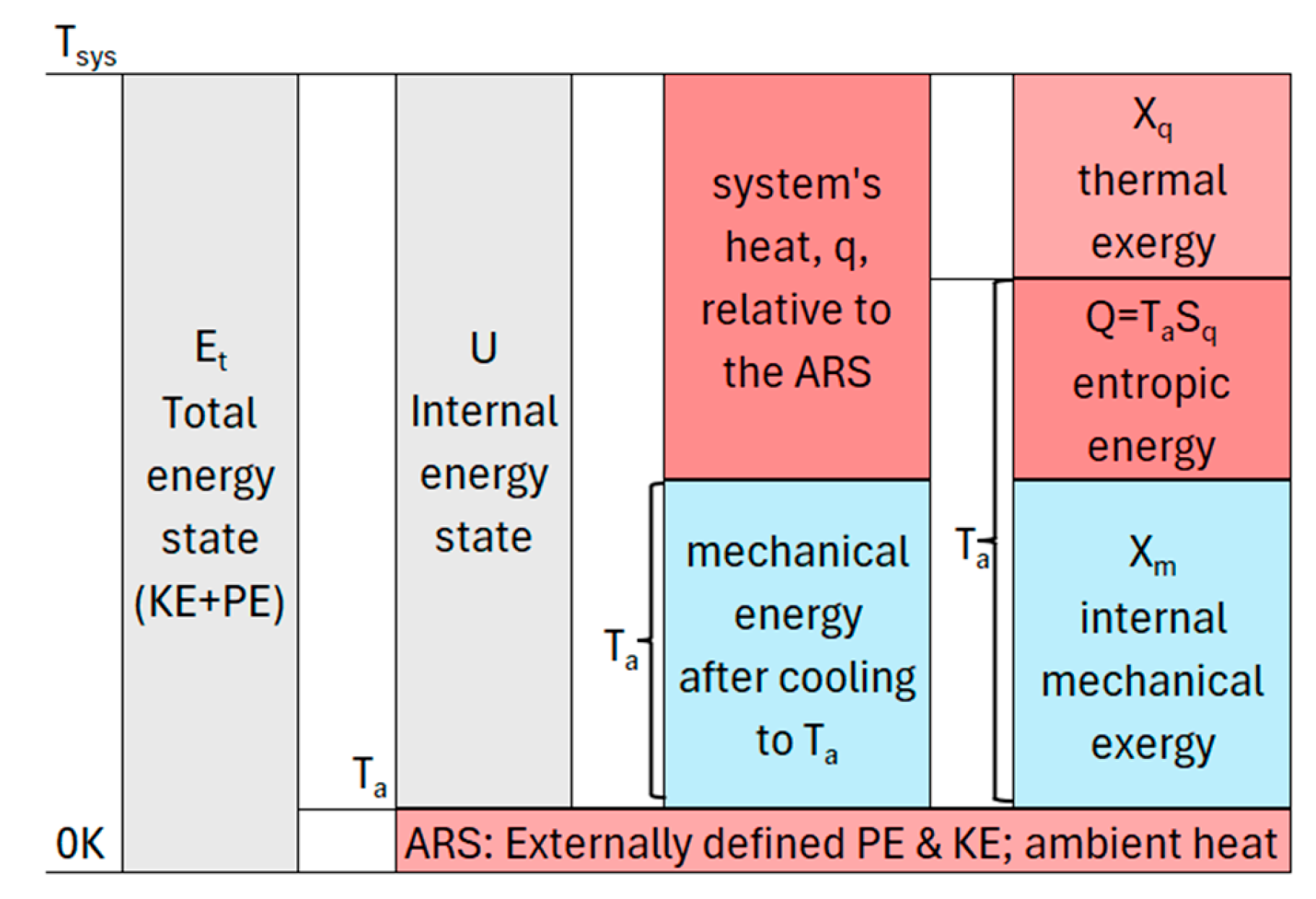
Figure 2.
Microstate and macrostate energy states. The macrostate resolves the microstate’s exergy into accessible and inaccessible energy with respect to its FIR. At time zero, the macrostate’s FIR is set to the system’s initial ARS and it is given complete information (Scf = 0). Temperature declines in the system or its ambient surroundings, dissipation, and information loss from random transitions change the energy states for the system and its macrostate description.
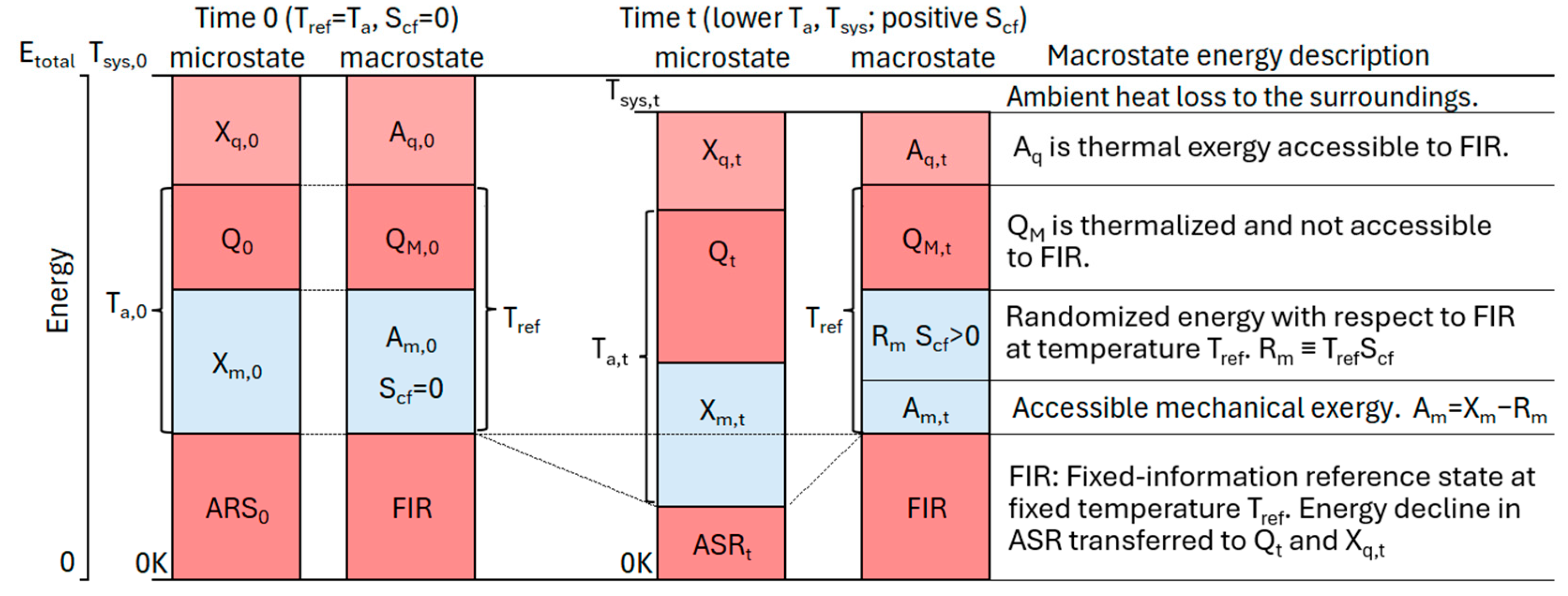
Figure 3.
State Transitions. (A) Random Energy-State transition. (B) Random instantiation and observation of a polarized photon.
Figure 3.
State Transitions. (A) Random Energy-State transition. (B) Random instantiation and observation of a polarized photon.
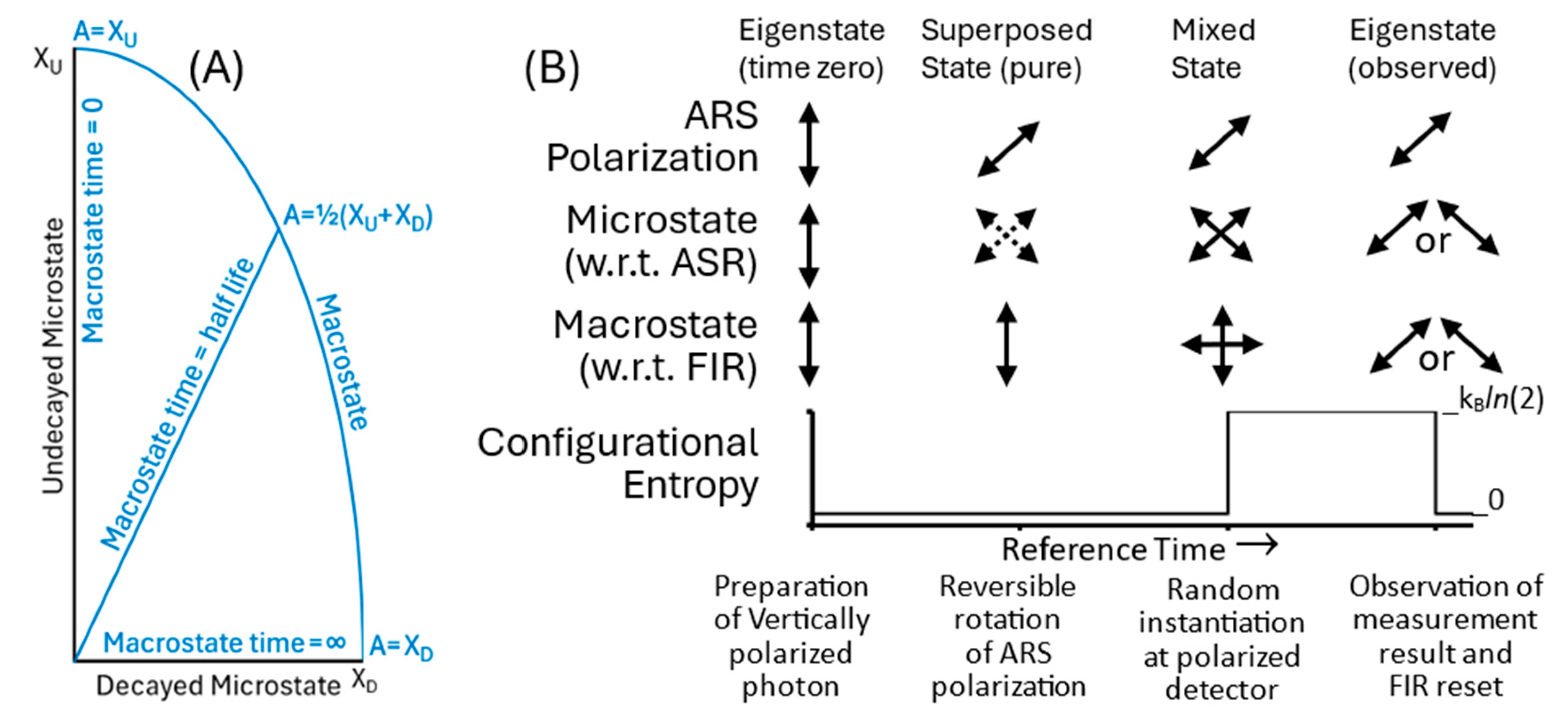
Figure 4.
Entangled Photons are emitted from a source in opposite directions. Photons are unpolarized prior to measurement. The arrows at time 1 show the superposition of virtual polarized-particle potentialities, based on the detector orientation. The photons simultaneously appear at the detectors at time 2 with randomly instantiated, but anticorrelated, polarizations.
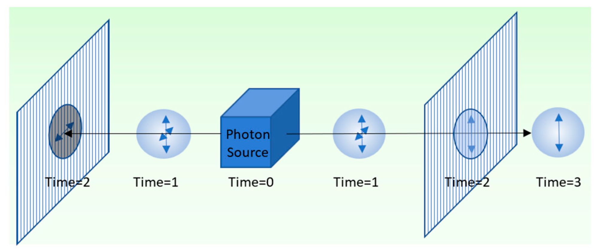
Figure 5.
Instantaneous Correlation of Spatially Separated Measurements. Photons emitted from the source S are simultaneously measured at points A and B at system time-zero (left axis). The shaded light cones expand from points A0 and B0 across space (projected onto the horizontal axis). Alice measures her photon at her reference time, tᵣ,0 and she measures Bob’s signal photon at tᵣ,1 (right vertical axis).
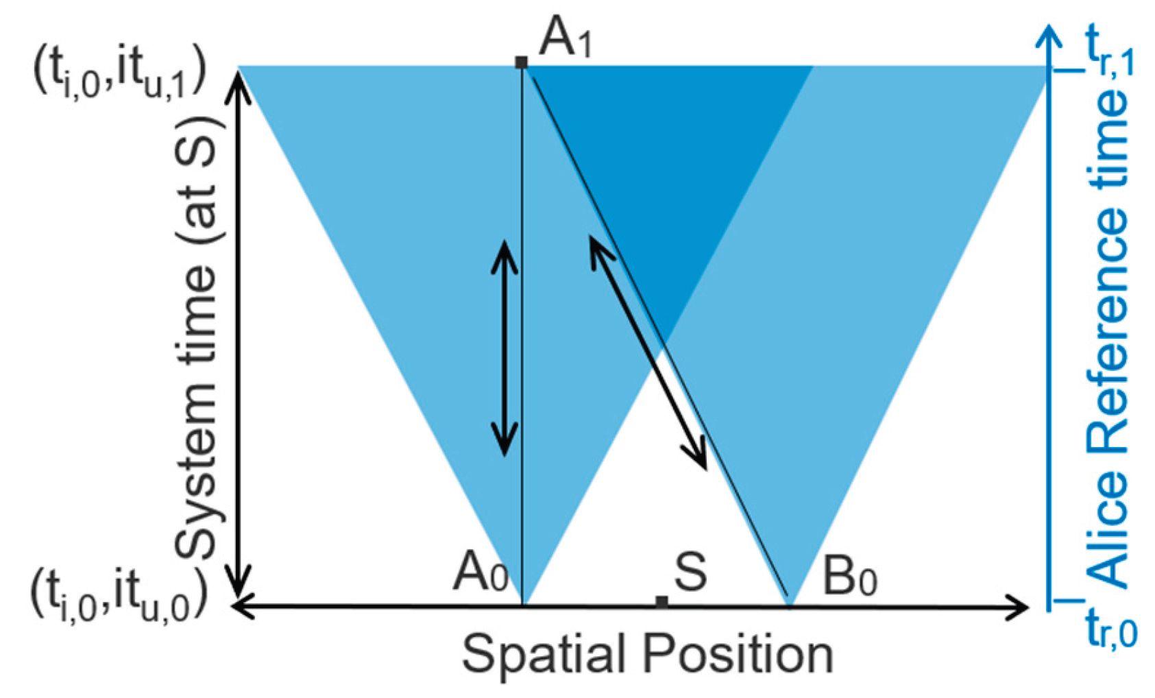

Table 1.
Summary of entropy definitions.
| Thermodynamic entropy |
|
Clausius’s original definition of thermodynamic entropy and 3rd Law entropy (CvdT = dq). |
| Thermal entropy (5) | TCM generalization of 3rd Law entropy | |
| Boltzmann entropy (10) |
Boltzmann statistical entropy, objectively based on zero prior information and unbiased equal probabilities. | |
| Configurational entropy (7) |
A generalized statistical entropy describing the uncertainty of measurement results for configurational or energy-state transitions. | |
| Bayesian Configurational entropy |
A subjective measure of uncertainty of a mixed state, based on an observer’s expectations of its message or state, without regard to its accuracy. | |
| Frequentist Configurational entropy |
An objective measure of the loss in accuracy of predicted measurement results, based on a system’s frequentist transition probabilities. |
Disclaimer/Publisher’s Note: The statements, opinions and data contained in all publications are solely those of the individual author(s) and contributor(s) and not of MDPI and/or the editor(s). MDPI and/or the editor(s) disclaim responsibility for any injury to people or property resulting from any ideas, methods, instructions or products referred to in the content. |
© 2025 by the authors. Licensee MDPI, Basel, Switzerland. This article is an open access article distributed under the terms and conditions of the Creative Commons Attribution (CC BY) license (http://creativecommons.org/licenses/by/4.0/).
Copyright: This open access article is published under a Creative Commons CC BY 4.0 license, which permit the free download, distribution, and reuse, provided that the author and preprint are cited in any reuse.


