Submitted:
30 September 2025
Posted:
01 October 2025
You are already at the latest version
Abstract
We consider detailed cosmological tests of dark energy models obtained from the general conformal transformation of the Kropina metric, representing an (α,β)-type Finslerian geometry. In particular, we restrict our analysis to the osculating Barthel-Kropina geometry. The Kropina metric function is defined as the ratio of the square of a Riemannian metric α and of the one-form β. In this framework we also consider the role of the conformal transformations of the metric, which allows to introduce a family of conformal Barthel–Kropina theories in an osculating geometry. The models obtained in this way are described by second-order field equations, in the presence of an effective scalar field induced by the conformal factor. The generalized Friedmann equations of the model are obtained by adopting for the Riemannian metric α the Friedmann-Lemaitre-Robertson-Walker representation. In order to close the cosmological field equations we assume a specific relationship between the component of the one-form β and the conformal factor. With this assumption, the cosmological evolution is determined by the initial conditions of the scalar field and a single free parameter of the model. The conformal Barthel-Kropina cosmological models are compared against several observational datasets, including Cosmic Chronometers, Type Ia Supernovae, and Baryon Acoustic Oscillations, using a Markov Chain Monte Carlo (MCMC) analysis. A comparison with the predictions of standard ΛCDM model is also performed.
Keywords:
Barthel connection
; (α
; β) metrics
; Finslerian Cosmology
; Posterior Inference
; MCMC statistical analysis
1. Introduction
The investigation of the role of the conformal transformations in physics may provide an important avenue for the understanding of gravitational phenomena, of the elementary particle physics, and of their relationship. The idea of the conformal transformations (rescalings) was first proposed by Weyl [1,2,3], in his attempt for finding a unified theory of gravitation and electromagnetism. The conformal transformations were called by Weyl gauge transformations, and they are presently a standard method in elementary particle physics. Gauge field theories are the basic theoretical tool of our present day approach to field theory, and they give deep insights into the properties of the elementary particles. In gravitational theories, the Weyl gauge transformations are called conformal transformations. The invariance of physical laws under conformal transformations is called conformal invariance. Many important geometrical quantities are also conformally invariant. Many important equations of physics, including the Maxwell equations, satisfy the requirement of local scale invariance.
The important role of conformal transformations was emphasized by T. Hooft in [4,5], who pointed out that conformal symmetry may be an exact symmetry of nature, which is broken spontaneously. Conformal symmetry could be as important as the Lorentz symmetry of the laws of nature, and it may open some new directions for the understanding of the physics of the Planck scale. In a theory of the gravitational interaction proposed in [5] it is assumed that local conformal symmetry is an exact, but spontaneously broken symmetry of nature. The conformal part of the metric is interpreted as a dilaton field. The theory has intriguing implications, and it suggests that black holes are topologically trivial, regular solitons, without singularities, firewalls, or horizons.
The role of the conformal transformations was also explored by Penrose [6,7,8,9], in the framework of a cosmological model called Conformal Cyclic Cosmology (CCC). The starting point of this model is the observation that when the de Sitter accelerating stage, induced by the presence of the positive cosmological constant , ends, the spacetime is conformally flat, and space-like. This geometric structure coincides with the geometry of the initial boundary of the Universe after the Big Bang. Moreover, in the Conformal Cyclic Cosmology model it is suggested that the Universe consists of eons, time oriented manifolds, possessing spacelike null infinities. Conformally invariant gravitational theories were investigated in [10,11,12,13,14,15,16,17,18,19,20,21,22,23,24,25,26].
In 1918, in the year Weyl presented his extension of Riemann geometry, another important geometric theory was also introduced. This is the Finsler geometry [27], representing another important generalization of Riemann geometry. Even that from a purely mathematical perspective Finsler geometry is ”... just Riemannian geometry without the quadratic restriction” [28], we will still consider Finsler geometry as a generalization of Riemann geometry. The Finsler geometry was already anticipated by Riemann [29], who in a general space introduced a geometric structure given by . According to this definition, for a nonzero , the function , the Finsler metric function, must be a positive function defined on the tangent bundle TM. must also satisfy the important requirement of homogeneity of degree one in y, which implies the condition , where is a positive constant. The case leads to the limiting case of the Riemann geometry [30,31].
An important class of Finsler spaces is represented by the Kropina spaces [32,33]. The Kropina spaces are Finsler spaces of the type , in which the Finsler metric function F is defined as , where denotes a Riemannian metric, , and is an one-form. The properties of the Kropina spaces have been considered, from a mathematical perspective, in [34,35,36,37,38,39,40]. A significant simplification of the mathematical approach can be obtained through the use of the theory of the osculating Riemann spaces of Finsler geometries, introduced in [41,42]. In this approach one replaces a complex Finsler geometric object with a simpler mathematical object, represented, for example, by a Riemann metric. Thus, by using the osculating formalism, a simpler mathematical and geometrical description can be obtained. In the specific case of the Kropina metric, one can take the field as , and then the A-osculating Riemannian manifold is defined as . Moreover, one can associate to this mathematical structure the Barthel connection, representing the Levi-Civita connection of the Riemann metric .
One of the most important scientific developments of the 20th century is represented by Einstein’s theory of General Relativity (GR). Its remarkable success is mainly due to the introduction of the geometric description of the gravitational interaction [43,44]. GR is a fundamental theory of matter, gravity, and space-time, matter, and of their interaction, giving an extremely precise description of the gravitational effects at the level of the Solar System. Unfortunately, when extended to very small, and very large astrophysical or cosmological scales, GR is confronted with several challenges, coming mostly from quantum field theory and cosmology.
First of all, a large number of recent cosmological observations have raised important concerns about the possibility of considering GR as the theoretical foundation of cosmology. The recent acceleration of the Universe [45,46,47] can be explained remarkably well by reintroducing in the Einstein field equations the cosmological constant [48], together with another mysterious, and yet undetected, matter component, called dark matter, a pressureless, and cold constituent of the Universe. In recent years the CDM ( Cold Dark Matter) cosmological model has become a standard approach for the analysis and interpretation of the observational cosmological data. In this direction, the CDM model proved to be very successful. However, there are a number of important questions suggesting that CDM may be considered as only representing a first order approximation of a more general model, not yet known [49].
One of the basic challenges the CDM model faces is the lack of a consistent physical and theoretical background, related to the absence of a convincing explanation or description of the cosmological constant. Presently, no convincing physical or geometrical interpretation of is known. Another weakness of the CDM model is related to the nature of dark matter. After many years of intensive observational and experimental efforts, no positive detection of the particles associated to dark matter has been yet recorded in both terrestrial experiments, or astrophysical observations.
The technological advances in the field of cosmology, which led to the significant increase of the precision of observations, revealed an other important weakness of the CDM standard model. Significant deviations have been found between the Hubble expansion rates obtained from the low redshift (local) measurements and those measured by the Planck satellite experiment by using the Cosmic Microwave Background Radiation (CMBR). The differences obtained from the different determinations of the values of the present day Hubble constant are usually called the Hubble tension, and, if confirmed, it could represent a paradigmatic crisis in present day cosmology [50,51,53,54,55,56]. The difference in the numerical values of obtained by the Planck satellite, km/ s/ Mpc [55,56], and the values of km/ s/ Mpc [53] inferred by the SH0ES collaboration, is greater than 3[56]. If it indeed exists, the Hubble tension is a strong indicator of the need of developing new gravitational theories, and for the necessity of replacing the CDM model with an alternative and more realistic one.
General relativity also faces important challenges on a theoretical ground. The Big Bang singularity, and generally the presence of singularities in the theory, which are extremely important for the understanding of the origin of the Universe, and of its very early evolution, is still unexplained by general relativity, and the CDM cosmology. Moreover, GR cannot describe the extremely high density phases of matter, in the presence of extremely strong gravitational fields, as is the case for black holes. From another theoretical perspective, very little progress has been made, if any, in the understanding of the quantum properties of gravity, including the quantization of geometry, spacetime, and gravity [57]. Therefore, in the absence of a quantum description of gravity, as yet GR cannot be considered as a fundamental physical theory, similar to the theories describing elementary particle interactions, and their properties.
One possibility to obtain a solution of these fundamental problems is to consider generalized theories of gravity, which contain GR as a particular case, corresponding to a weak field limit. There are many attempts for constructing alternative theoretical approaches to GR. These novel theories are obtained by introducing and developing different physical and mathematical approaches (for detailed reviews of modified gravity theories, and of their cosmological and astrophysical implications see [58,59,60,61].
One of the interesting extensions of standard general relativity are represented by gravitational theories based on the extensive use of Finsler geometry. Finsler type gravitational theories, as well as the cosmological models obtained by using this geometrical structures represent important alternatives to standard cosmology. Generally, they can provide a geometric explanation of dark energy, and even of dark matter. Many studies have been devoted to the applications of the Finsler geometry in cosmology and gravitational physics. These studies have led to a new understanding and to a new geometric perspective on the cosmological evolution, dark energy, and dark matter [62,63,64,65,66,67,68,69,70,71,72,73,74,75,76,77]. For a recent review of the cosmological applications of the Finsler geometry see [78].
In particular, a special type of Finsler geometry, the Barthel-Kropina spaces, have been also investigated extensively from the point of view of their cosmological applications [79,80,81]. The Barthel–Kropina cosmological approach is generally based on the introduction of a Barthel connection in an osculating type Finsler geometry. The Barthel connection has the important property that it is the Levi-Civita connection of a Riemannian metric. By assuming that the background Riemannian metric is of the Friedmann–Lemaitre–Robertson–Walker type one can obtain the generalized Friedmann equations of the Barthel–Kropina models. These equations show that an effective geometric dark energy component can be generated within the framework of the Barthel-Kropina geometries, having an effective, geometric type energy density and pressure, respectively. To fully solve the cosmological models generally one must impose an equation of state for the dark energy.
A specific Barthel-Kropina type cosmological model was considered in [81]. The model was obtained from the general conformal transformation of the Kropina metric, and the possibilities of obtaining conformal theories of gravity in the osculating Barthel–Kropina geometric framework were investigated. A family of conformal Barthel–Kropina gravitational field theories in an osculating geometry with second-order field equations were introduced. The models depend on the properties of the conformal factor, whose presence leads to the appearance of an effective scalar field of geometric origin in the gravitational field equations. The cosmological implications of the theory were investigated in detail by assuming a specific relation between the component of the one-form of the Kropina metric and the conformal factor. The cosmological evolution is thus determined by the initial conditions of the scalar field and a free parameter of the model.
It is the goal of the present paper to extend the investigations initiated in [81], by considering a detailed analysis of the cosmological tests, including a full comparisons with observational data of this dark energy model are considered in detail. To constrain the conformal Barthel–Kropina model parameters, and the values of the scalar field, we use 57 Hubble data points, the Pantheon Supernovae Type Ia data sample,and the BAO (Baryonic Acoustic Oscillations) measurements. The statistical analysis is performed by using Markov Chain Monte Carlo (MCMC) simulations. A detailed comparison with the standard CDM model is also performed, with the Akaike information criterion (AIC), and the Bayesian information criterion (BIC) used as the two model selection tools. The statefinder diagnostics consisting of jerk and snap parameters, and the diagnostic tools are also considered for the comparative study of the conformal Barthel–Kropina and CDM cosmologies. Our results indicate that for certain values of the model parameters the Barthel–Kropina dark energy model gives a good description of the observational data, and thus it can be considered a viable alternative of the CDM model, by also alleviating some of the theoretical problems standard cosmology is facing.
The present paper is organized as follows. The theoretical foundations of the conformal Barthel-Kropina type gravitational theories are introduced in Section 2, where the generalized Friedmann equations are also written down. The cosmological tests of the theory are considered, for a few values of the model parameter, in Section 3. A summary and a discussion of the cosmological implications of the theory is presented in Section 4. We conclude the results of our investigations in Section 3.2.
2. Conformal Barthel–Kropina Cosmology
In the present Section, by following the approach initiated in [81], we will introduce the fundamentals of the conformal transformations in Riemann and Barthel-Kropina geometries, respectively, and we will present the generalized Friedmann equations of the osculating conformal Barthel-Kropina geometry.
2.1. Conformal Transformations in Riemann Geometry
The conformal transformation of a Riemannian metric , defined as [44]
where is an arbitrary function of the coordinates x, plays an important role in both mathematics and physics. In Riemannian geometry the conformal transformations are defined on the space-time manifold M, and denotes the conformally transformed Riemannian metric. The Christoffel symbols of and , and , respectively, are then related as
where where
For the transformation law of the covariant derivative for any we obtain the expression [81]
where we have denoted
2.1.1. Matter and Energy-Momentum Tensor
In standard general relativity the matter action can be generally written in the form [43,44]
where is the matter Lagrangian, which we consider to be a function of the metric tensor g, and of the matter fields , which can be of bosonic or fermionic nature. We assume that under conformal transformations the matter Lagrangian transforms according to the rule
and thus the conformally transformed action takes the form [81]
Thus, the action of the ordinary baryonic matter is invariant under the conformal transformations (7). This important result indicates that since the baryonic matter action is an invariant quantity, in all conformally related frames it can be described by the same expression.
The matter energy-momentum tensor is defined as [44]
and, after a conformal transformation of the metric it becomes [81]
The trace of the baryonic matter energy-momentum tensor transforms in a conformal transformation as , where .
2.2. The Osculating Barthel-Kropina Cosmological Model
The Kropina metric function, a specific Finsler type metric, is defined according to [81]
We also denote . The fundamental tensor associated to the metric is given by [81]
For the Riemannian metric we consider the expression
which describes the homogeneous and isotropic, flat Friedmann-Lemaitre-. For the one-form we adopt the expression , where
is a covariant vector field defined on the base manifold M.
We also consider the preferred direction
where . For the case of the FLRW metric we have [81]
where is an arbitrary function of the time coordinate .
We can now obtain
and
where , .
By substituting the above relations in (12), we obtain the osculating Riemannian metric of the Barthel-Kropina cosmological model as [81]
The Einstein field equations are given by
and
respectively, where and p denote the matter energy density, and pressure, respectively. Hence, the system of the generalized Friedmann equations in the osculating Barthel-Kropina geometry take the form [81]
where . By substituting the term and with the use of Eq. (22), it follows that Eq. (23) can be simplified to
2.3. The Conformal Osculating Barthel-Kropina Model-the Generalized Friedmann Equations
For a general -metric with metric function , we introduce the conformal transformation [81]
which is an -metric, where
The fundamental tensor of is given by the Hessian
The conformally transformed osculating Riemannian metric is obtained in the form
where is given by Eq. (19). Explicitly, the metric has the expression
2.4. The Generalized Friedmann Equations
We assume now that the Einstein gravitational field equations are given in the conformal osculating Barthel-Kropina as [81]
where by we have denoted the matter energy-momentum tensor in the conformal frame. We further assume that the thermodynamic properties of the baryonic matter in the conformal Barthel-Kropina cosmological models can be described by the conformal energy density , and the conformal thermodynamic pressure only. We also introduce another important assumption, namely, we postulate the existence of a coordinate frame comoving with matter. Therefore, the energy-momentum tensor of the baryonic matter takes in the conformal frame the form
and
respectively.
The homogeneity and isotropy of the space-time implies that all physical and geometrical quantities can depend only on the time coordinate . Moreover, we assume that the conformal factor has the form [81]
where , are arbitrary constants. For this choice the Einstein field equations give , which leads to , . Therefore, without any loss in generality we chose the conformal factor as , and thus in the following we consider only time dependent conformal transformations of the Kropina metric [81].
2.5. The Generalized Friedmann Equations
By taking into account all the above results, it follows that the generalized Friedmann equations, in the conformal osculating Barthel-Kropina cosmology take the form [81]
and
respectively. After eliminating the term between Eqs. (36) and (37) we obtain the equation
We consider now the possibility of the description of the dark energy as a geometric effect in the Barthel-Kropina cosmological model [81]. In the limit , and , we recover the standard general relativistic model without a cosmological constant. The deviations from general relativity,a nd standard Riemannian geometry can be considered as a small variation of , depending on the conformal factor. Thus, we introduce a cosmological model in which is given by [81]
where is a constant.
The generalized Friedmann equations (36) and (37) of the conformal osculating Barthel-Kropina model take the form
and
respectively, where we have introduced the notations
and
respectively.
The total conservation equation for matter and the conformally induced scalar field can be obtained from the generalized Friedmann equations in the form
Equation (44) can be split into two independent balance equations, one for matter, and the second for the conformal scalar field, respectively, which take the form
and
respectively. From Eq. (46) we obtain the time evolution of the conformal scalar field as
Thus, the basic equations describing the cosmological dynamics in the conformal Barthel-Kropina model are given by Eqs. (40), (41) and (47), respectively [81].
We introduce now in the generalized Friedmann equations instead of the coordinate the time t, and instead the Hubble function the time dependent Hubble function , where by a dot we have denoted the derivative with respect to the cosmological time t. Hence we have . We introduce now a set of dimensionless variables , defined as
where is the present day value of the Hubble function. Hence, the full set of the evolution equations of the conformal osculating Barthel-Kropina cosmological model is obtained in the form
and
respectively.
After integrating Eq. (51) for the matter density, we obtain
where is an arbitrary constant of integration.
Next, in order to obtain a form of the evolution equations that allow an easy comparison with the observational data we introduce the redshift variable z defined as , with ( for simplicity). Therefore, the cosmological evolution equations in the redshift space take the form [81]
and
respectively. The system of equations (55)-(58) must be integrated with the initial conditions , , , and , respectively.
3. Observational Tests of the Conformal Barthel-Kropina Cosmological Models
In this Section, we present constraints on the parameters of the conformal oscillating Barthel–Kropina cosmological model. To do this, we use the cosmological model proposed by the following set of differential equations (55)–(58). In the following analysis, we plug the to the values 1, , and . We then perform MCMC analysis to constrain the parameters of the conformal Barthel–Kropina cosmological models. The cosmological model corresponding to the value is given by
The system of cosmological evolution equations (58)-(61) must be integrated with the initial conditions , , , and , respectively.
3.1. Methodology and Datasets
To constrain the parameters of the Conformal Barthel–Kropina Cosmological Model. We first solve the system of differential equations of the conformal oscillating Barthel–Kropina cosmological model given by Eqs. (55)–(58) by specifying appropriate initial conditions and integrating over the redshift z. The system of equations is then numerically integrated over the redshift interval using the solve_ivp routine with the Radau method, which is an implicit Runge–Kutta solver particularly well suited for stiff systems of differential equations. Then we use the numerical solution obtained above and apply the Nested Sampling algorithm, implemented with the PyPolyChord library, to constrain the parameters of the conformal oscillating Barthel–Kropina cosmological model.1 [82,83].
Nested sampling is particularly well suited for cosmological inference, as it not only provides robust posterior distributions for parameter estimation but also directly computes the Bayesian evidence, . In this framework, the posterior probability distribution is expressed as where is the likelihood, is the prior, and is the evidence obtained by marginalizing over the full parameter space,
Beyond parameter estimation, the evidence plays a key role in model selection. Competing cosmological models are compared using the Bayes factor, which quantifies the statistical preference of one model over another.
To interpret the strength of the evidence, we follow the Jeffreys’ scale [84]: indicates inconclusive or weak support, corresponds to moderate evidence, suggests strong evidence, and is regarded as decisive in favor of the model with higher evidence.
In our analysis, we employ PyPolyChord with 300 live points to ensure robust Bayesian evidence estimation. For visualization, we use the getdist package2 [85], which provides marginalized posterior distributions and parameter correlation plots. The study incorporates multiple dataset combinations, including Baryon Acoustic Oscillation measurements, Type Ia supernovae, and Cosmic Chronometers, as detailed below.
- Baryon Acoustic Oscillation : We use the Baryon Acoustic Oscillation (BAO) measurements from over 14 million galaxies and quasars provided by the Dark Energy Spectroscopic Instrument (DESI) Data Release 2 (DR2)3[86]. To constrain cosmological parameters using BAO from DESI DR2, we compute three primary distance measures: the Hubble distance , the comoving angular diameter distance , and the volume-averaged distance . These distances are expressed as ratios , , and for direct comparison with the observed BAO data. Here, denotes the sound horizon at the drag epoch (), defined as , where is the sound speed of the photon–baryon fluid. While the standard flat CDM model predicts Mpc [87], we treat as a free parameter in our analysis [88,89,90,91,92].
- Type Ia supernova : We also use the Pantheon+ (PP) CosmoSIS likelihood 4in our analysis, which accounts for both statistical and systematic uncertainties through a covariance matrix [93]. This dataset includes 1,590 light curves from 1,550 Type Ia Supernovae (SNe Ia) spanning the redshift range [94]. Light curves at are excluded due to significant systematic uncertainties arising from peculiar velocities. In this analysis, we also marginalize over the parameter ; for further details, see Equations (A9–A12) of [95].
- Cosmic Chronometers : We also use Hubble measurements obtained through the differential age method. This technique relies on passively evolving massive galaxies, formed at redshifts , providing a direct, model-independent estimate of the Hubble parameter via the relation [96]. In this analysis, we use the likelihood provided by Moresco on his GitLab repository5, which incorporates the full covariance matrix to account for both statistical and systematic uncertainties [97,98]. This likelihood includes Hubble parameter measurements spanning the redshift range [99,100,101].
To constrain the parameters of each cosmological model, we maximize the overall likelihood function, which is defined as:
3.2. Comparing Conformal Barthel–Kropina with CDM Model
In this subsection, we plot the Hubble function and its residuals with respect to redshift, after obtaining the mean value of each Conformal Barthel–Kropina cosmological model for different values of . We then compare these results with the CDM model and the CC measurements proposed by [99,100,101]. This analysis allows us to identify which Conformal Barthel–Kropina model, for a given value of , is most compatible with the CDM framework and the observational datasets.
3.2.1. Evolution of the Hubble Parameter and Hubble Residual
In this section, we compare the Conformal Barthel–Kropina models for different values of against the CDM model and the CC measurements. As a first step, we plot the CDM model using the following Hubble function:
where and .
In the case of the Conformal Barthel–Kropina models, we consider the system of differential equations given in Eqs. (55)–(58). We obtain the numerical solution of these equations using the initial conditions derived from the MCMC simulations. The resulting numerical solution, denoted by , is then scaled by the factor , yielding the final form of the Hubble function: Furthermore, the Hubble residual is defined as
where denotes the Hubble parameter predicted by the Conformal Barthel–Kropina model for , , and , and is the Hubble parameter predicted by the standard CDM model.
These comparisons allow us to quantify the deviations of the Conformal Barthel–Kropina models from the standard CDM predictions. By examining both the Hubble function and the residual , we can assess how well each model fits the observational data and determine which values of provide closer agreement with current cosmic chronometer measurements. This analysis thus provides insight into the potential viability of the Conformal Barthel–Kropina framework as an alternative cosmological model.
3.3. Cosmographic Analysis of Conformal Barthel–Kropina with CDM Model
Cosmography serves as a robust, model-independent tool to probe the dynamical features of the Universe by expanding cosmological observables with respect to redshift. This approach does not rely on the underlying gravitational theory or specific assumptions about dark energy components, but rather on the kinematic properties of the cosmic expansion. The formalism uses the Taylor expansion of the scale factor around the present epoch, expressing the expansion history in terms of measurable quantities like the Hubble parameter , the deceleration parameter , and higher-order derivatives such as the jerk parameter , the snap parameter , and the lerk parameter [102,103,104,105].
3.3.1. Deceleration Parameter and Jerk Parameter
The deceleration parameter is mathematically expressed as:
where is the Hubble parameter at redshift z. A negative implies accelerated expansion, whereas a positive value suggests a decelerating universe. Two significant cosmographic markers derived from include the present-day value , representing the current expansion state, and the transition redshift , defined by , which marks the epoch where the Universe shifted from deceleration to acceleration.
The jerk parameter, capturing the rate of change of acceleration, is defined as:
In the standard CDM cosmological model, remains constant at , independent of redshift. Deviations from this value indicate the presence of additional dynamical effects beyond the cosmological constant. The plots presented in Fig showcase the numerical evaluation of and for different values of in the conformal Barthel–Kropina model, alongside the CDM baseline.
3.4. Dimensionless Matter Density and Conformal Factor
The dimensionless matter density is a fundamental cosmological parameter that provides a key test of the consistency of different cosmological models. It accounts for the total matter content of the Universe, including both baryonic and dark matter, and its present-day value sets the initial conditions for the Universe’s cosmological evolution. While cosmological models do not predict the current matter density directly, they describe how it evolves during the earlier stages of the Universe.
The conformal factor arises from conformal transformations in geometry and physics, which modify the metric in a way that preserves angles but not necessarily lengths. In practical terms, the conformal factor is a function that rescales the metric at every point, allowing shapes to stretch or shrink while keeping the local angle structure intact. This factor plays an important role in modeling the geometrical and physical properties of spacetime in various cosmological frameworks.
3.5. Model Selection and Statistical Assessment for Conformal Barthel–Kropina Models
In this section, we use statistical metric to evaluate the performance and complexity of the Conformal Barthel–Kropina models for , -1, and 4/3. These tests quantify how well the models fit the observational data, compare them to CDM, and determine whether the additional parameters significantly improve the fit without adding unnecessary complexity.
3.5.1. Goodness of Fit
First, we use the chi-squared statistic, , to evaluate the performance of the Conformal Barthel–Kropina model, as it quantifies the discrepancy between theoretical predictions and observational data. To account for models with different numbers of free parameters, we consider the reduced chi-squared:
where DOF is the number of data points minus the number of fitted parameters. Values of indicate a good fit, significantly higher values suggest a poor fit, and much lower values may signal overfitting.
3.5.2. Model Comparison Using Information Criteria
Then we use information criteria to evaluate both the goodness of fit and the complexity of the Conformal Barthel–Kropina model relative to CDM. These criteria are based on the minimum chi-squared value, , and include the Akaike Information Criterion (AIC) and the Bayesian Information Criterion (BIC) [107,108,109,110,111], defined as:
where is the number of free parameters, is the total number of observational data points ( in our analysis), and represents the minimum chi-squared achieved by the model. Both criteria penalize models with more parameters to avoid overfitting, with BIC generally applying a stronger penalty for larger datasets. For reference, the CDM model has 3 free parameters, while the Conformal Barthel–Kropina model considered here has 5 free parameters.
3.5.3. Relative Comparison: AIC and BIC
To compare the Conformal Barthel–Kropina model directly with CDM, we compute the differences:
The interpretation follows the Jeffreys’ scale [84]:
- : Models are statistically comparable.
- : Considerably less support for the model.
- : Strongly disfavored.
- : Weak evidence against the model.
- : Moderate evidence against the model.
- : Strong evidence against the model.
We also evaluate the statistical significance of the fit using the p-value:
where is the cumulative chi-squared distribution with degrees of freedom (data points minus free parameters). A p-value indicates that the model provides a statistically significant fit. In our analysis, the degrees of freedom (DOF) is 1615 for the CDM model and 1614 for the Conformal Barthel–Kropina model for each value of
4. Summary and Discussion of the Results
In the present Section, we discuss the main results obtained by confronting the proposed cosmological models with observations, and by comparing their predictions and statistical significance with those of the CDM model.
4.1. MCMC Results
Figure 1 shows the triangle plots for the Conformal Barthel–Kropina cosmological models for different values of . The diagonal panels display the one-dimensional marginalized posterior distributions for each parameter, while the off-diagonal panels present the two-dimensional marginalized confidence contours at 68% and 95% levels. Table 1 summarizes the numerical constraints obtained for the different variants of the Conformal Barthel–Kropina models as well as for the CDM model.
We first compare the predicted values of the CDM model obtained by including the DESI DR1 and PP datasets. When considering only the CC measurements, we find
which is consistent with the results reported in [99,100,101]. For the Conformal Barthel–Kropina models, we obtain the following values:
- for , ,
- for , ,
- for , .
One can observe that the predicted values from the Conformal Barthel–Kropina models show only small deviations from the CDM prediction. Specifically, the shifts correspond to for , for , and for
Further, by including the DESI DR2 and PP datasets together with the CC measurements, we find that the deviations of the best-fit values for the Conformal Barthel-Kropina models from the predicted CDM value remain small. Specifically, the shifts correspond to for , for , and for . Since all these deviations are below the level, the Conformal Barthel-Kropina models show no statistically significant tension with the CDM prediction of when DESI DR2 and PP are combined with the CC dataset.
Similarly, for the , we find similarly small deviations from the CDM prediction. In particular, the shifts correspond to for , for , and for . These results indicate that the Conformal Barthel-Kropina models are consistent with the CDM prediction for the sound horizon, with all deviations lying well below the level. In addition, the predicted values of in each variant of the Conformal Barthel-Kropina models are found to be close to those reported by [87].
4.2. Hubble Parameter, and Hubble Residual Results
Figure 2 shows the evolution of the Hubble function and Hubble residuals. It can be observed that the Conformal Barthel-Kropina model for shows close agreement with the CDM model. In contrast, the cases and show noticeable deviations from CDM, though at very low redshift they also converge back to similar behavior. This trend is similarly reflected in the Hubble residuals
4.3. Cosmographic Results
Figure 3 shows the evolution of Cosmographic parameters. The left panel shows the evolution of deceleration parameter . The CDM shows smooth transition from positive at higher redshift to negative values at lower redshift, consistent with observations of late-time acceleration. For , the model closely follows the CDM trend, but at low redshift it shows similar behavior to CDM. The case shows a more rapid transition to acceleration, suggesting a Universe that has undergone earlier acceleration phases. Meanwhile, results in a slower transition, with the deceleration parameter remaining positive over a wider range of redshift, indicating prolonged decelerated expansion before transitioning to acceleration. The right panel shows the evolution of Jerk parameter , where the CDM model remains flat at as expected. The Barthel–Kropina models, however, exhibit distinct departures. The scenario stays nearly constant but presents slight deviations at higher redshifts, hinting at subtle dynamical corrections. The case shows a steadily increasing jerk parameter, pointing toward dynamic acceleration behavior not captured by the cosmological constant. The model shows a marked increase in jerk at higher redshift, signifying potential complexities in the expansion history that could be linked to evolving geometrical or matter contributions.
4.4. Dimensionless Matter Density and Conformal Factor Results
Figure 4 shows the variation of the baryonic matter content in the CDM and the Conformal Barthel–Randers models for different values of . In the left panel, it can be observed that in the case of , at the present epoch the baryonic matter content appears much lower than in the CDM prediction. On the other hand, for the model predicts values similar to the CDM model, and a comparable behavior can also be seen for .
While on the right panel we can see the variation of the conformal factor . For , at higher redshifts it predicts larger negative values; as the redshift decreases, increases rapidly and eventually takes positive values. On the other hand, for the model predicts positive values throughout the redshift range, while in the case of , it predicts negative values.
4.5. Statistical Results
Based on the statistical metrics presented in Table 2, we compare the performance of the Conformal Barthel–Kropina models for , , and against the standard CDM model. All Conformal Barthel–Kropina model variants exhibit reduced chi-squared values , indicating a good overall fit to the observational data. Specifically, for , for , and for , all slightly lower than the CDM value of . This suggests that the Conformal Barthel–Kropina models provide a marginally better fit to the data, without overfitting despite having two additional free parameters compared to CDM.
Examining the information criteria, we find that the Conformal Barthel–Kropina models yield lower AIC values compared to CDM, with AIC = , , and for , , and , respectively. According to the Jeffreys’ interpretation, AIC values indicate strong support for the model relative to the reference; hence, all Conformal Barthel–Kropina variants are strongly favored over CDM in terms of AIC. For BIC, which penalizes model complexity more heavily, the results are mixed. The CBK model with has BIC = , suggesting moderate evidence in favor of the CBK model, while yields BIC = and gives BIC = , indicating weak or even moderate evidence against these variants when penalizing for additional parameters. This reflects the stronger BIC penalty for the two extra parameters in the Conformal Barthel–Kropina models.
All Conformal Barthel–Kropina variants achieve high p-values (), compared to for CDM, indicating that the CBK models are statistically consistent with the observational data and provide an acceptable fit.
The logarithm of the Bayes factor, , provides a complementary assessment of model preference. For the Conformal Barthel–Kropina models, we find (), (), and (), which, following Jeffreys’ scale, corresponds to decisive evidence in favor of the Conformal Barthel–Kropina models over CDM. This reinforces the conclusion from the AIC analysis, showing that the additional parameters in the CBK framework are justified by a substantially improved fit to the data.
5. Conclusions and Final Remarks
One of the fundamental assumptions, and results, of present day physics is that the gravitational interaction can be successfully described only in geometric terms. Despite the tremendous initial success of the Riemannian geometry in this field, the recent observational results suggest that general relativity, as well as its mathematical foundation, may require a straightforward extension, and generalization. Within the multiple possibilities offered by the many existing geometric formalisms, Finsler geometry seems to be an important candidate for the reconstruction of the fundamentals of the gravitational theories. In the present work we have investigated the cosmological implications, and tests, of a specific Finslerian type gravitational and cosmological model, the conformal Barthel-Kropina model, which is based on the extension through the introduction of a conformal transformation of the Barthel - Kropina models [81].
The Barthel-Kropina type cosmological model are based on three mathematical assumptions. The first one is the assumption the Finsler metric function, describing the properties of the gravitational interaction, is a Kropina type metric, with . Secondly, the osculating approach is adopted for the Finsler-Kropinsa metric, as a result of which one obtains the important result that the Finsler is transformed into a Riemannian metric . And, finally, the first two assumptions imply that the connection of the Finsler-Riemann metric is the corresponding Levi-Civita connection, which, in Finsler geometry, is called the Barthel connection. With the use of this connection, one can calculate the basic geometric quantities-curvature tensors and their contractions, and write down the generalized Einstein tensor. Once the field equations are obtained, one can proceed to the investigation of their cosmological and astrophysical properties.
An extension of the Barthel-Kropina type theories can be obtained by introducing a conformal transformation of the metric function of the Finsler space. We can define a conformal transformation in the Finsler geometry in the following way. Let and be two Finsler spaces defined on the same base manifold , where L is the Finsler metric function. If the angle between any two tangent vectors in is equal to the angle in , then is called conformal to . Moreover, the transformation is called a conformal transformation of the metric [81]. A conformal transformation implies the existence of a scalar function with the property . For the case of an metric, the condition is equivalent to , which implies , and .
From a physical point of view, the consideration of the conformal transformations leads to the introduction in the mathematical formalism of the Barthel-Kropina geometries of a new degree of freedom, a scalar field related to the conformal transformation. This allows to obtain an interesting cosmological model, in which by fixing the conformal factor in a simple way, one arrives to a model depending on a single independent parameter , which determines the components of the one-form as .
Once the theoretical model of the conformal Barthel-Kropina geometry is formulated, our main goal was, on one hand, to confront the model with the observations, and, on the other hand, to obtain the optimal value of the free parameter of the model . The cosmological solutions obtained for a small set of values of , were compared against several observational datasets, including Cosmic Chronometers, Type Ia Supernovae, and Baryon Acoustic Oscillations. For the statistical analysis Markov Chain Monte Carlo (MCMC) methods were used. The results were also compared with the predictions of the standard CDM model.
From the comparison with the observational data it turns out that the value of is favored by the cosmological data. On the other hand, the conformal field has an interesting variation, indicating an evolution from negative values at large redshifts of the order of to negative values at the present time. On the other hand, even small deviations from the value lead to significant differences with respect to the observations.
To conclude, our present results indicate that the conformal Barthel-Kropina cosmological models provide a satisfactory fit to the observational data, suggesting they represent a viable alternative to the standard cosmological models based on Riemannian geometry, and standard general relativity.
Institutional Review Board Statement
Not applicable.
Informed Consent Statement
Not applicable.
Data Availability Statement
The data underlying this article is already given with references during the analysis of this work.
Conflicts of Interest
The authors declare no conflicts of interest. The funders had no role in the design of the study; in the collection, analyses, or interpretation of data; in the writing of the manuscript; or in the decision to publish the results
References
- Weyl, H. Gravitation und Elektrizität. Sitzungsberichte der Königlich Preussischen Akademie der Wissenschaften zu Berlin 1918, 1918, 465. [Google Scholar]
- Weyl, H. Space, Time, Matter, Dover, New York, 1952.
- Scholz, E. The unexpected resurgence of Weyl geometry in late 20-th century physics. 2017; arXiv:1703.03187. [Google Scholar]
- ’t Hooft, G. Local conformal symmetry: The missing symmetry component for space and time. Int. J. Mod. Phys. D 2015, 24, 1543001. [Google Scholar] [CrossRef]
- ’t Hooft, G. Singularities, horizons, firewalls, and local conformal symmetry. 2015; arXiv:1511.04427. [Google Scholar]
- Penrose, R. Cycles of Time: An Extraordinary New View of the Universe, Bodley Head, London, UK, 2010.
- Gurzadyan, V. G.; Penrose, R. On CCC-predicted concentric low-variance circles in the CMB sky Eur. Phys. J. Plus 2013, 128, 22. [Google Scholar] [CrossRef]
- Bars, I.; Steinhardt, P. J.; Turok, N. Cyclic cosmology, conformal symmetry and the metastability of the Higgs. Physics Letters B 2013, 726, 50. [Google Scholar] [CrossRef]
- Penrose, R. On the Gravitization of Quantum Mechanics 2: Conformal Cyclic Cosmology. Foundations of Physics 2014, 44, 873. [Google Scholar] [CrossRef]
- Mannheim P., D.; Kazanas, D. Exact Vacuum Solution to Conformal Weyl Gravity and Galactic Rotation Curves. Astrophys. J. 1989, 342, 635. [Google Scholar] [CrossRef]
- Mannheim, P. D. Solution to the Ghost Problem in Fourth Order Derivative Theories. Found. Phys. 2007, 37, 532. [Google Scholar] [CrossRef]
- Mannheim, P. D. Making the Case for Conformal Gravity. Found. Phys. 2012, 42, 388. [Google Scholar] [CrossRef]
- Ghilencea, D. M. Weyl R2 inflation with an emergent Planck scale. JHEP 2019, 03, 049. [Google Scholar] [CrossRef]
- Ghilencea, D. M.; Lee, H. M. Weyl gauge symmetry and its spontaneous breaking in the standard model and inflation. Phys. Rev. D 2019, 99, 115007. [Google Scholar] [CrossRef]
- Ghilencea, D. M. Gauging scale symmetry and inflation: Weyl versus Palatini gravity. Eur. Phys. J. C 20121, 81, 510. [Google Scholar] [CrossRef]
- Ghilencea, D. M. Standard Model in Weyl conformal geometry. Eur. Phys. J. C 2022, 82, 23. [Google Scholar] [CrossRef]
- Harko, T.; Shahidi, S. Coupling matter and curvature in Weyl geometry: conformally invariant fR,Lm gravity. Eur. Phys. J. C 2022, 82, 219. [Google Scholar] [CrossRef]
- Harko, T.; Shahidi, S. Palatini formulation of the conformally invariant fR,Lm gravity theory. Eur. Phys. J. C 2022, 82, 1003. [Google Scholar] [CrossRef]
- Yang, J.-Z.; Shahidi, S.; Harko, T. Black hole solutions in the quadratic Weyl conformal geometric theory of gravity. Eur. Phys. J. C 2022, 82, 1171. [Google Scholar] [CrossRef]
- Ghilencea, D. M. Non-metric geometry as the origin of mass in gauge theories of scale invariance. Eur. Phys. J. C 2023, 83, 176. [Google Scholar] [CrossRef]
- Burikham, P.; Harko, T.; Pimsamarn, K.; Shahidi, S. Dark matter as a Weyl geometric effect. Phys. Rev. D 2023, 107, 064008. [Google Scholar] [CrossRef]
- Haghani, Z.; Harko, T. Compact stellar structures in Weyl geometric gravity. Phys. Rev. D 2023, 107, 064068. [Google Scholar] [CrossRef]
- Weisswange, M.; Ghilencea, D. M.; Stöockinger, D. Quantum scale invariance in gauge theories and applications to muon production. Phys. Rev. D 2023, 107, 085008. [Google Scholar] [CrossRef]
- Ghilencea, D. M.; Hill, C. T. Renormalization group for nonminimal ϕ2R couplings and gravitational contact interactions. Phys. Rev. D 2023, 107, 085013. [Google Scholar] [CrossRef]
- Oancea, M.; Harko, T. Weyl geometric effects on the propagation of light in gravitational fields. Phys. Rev. D 2024, 109, 064020. [Google Scholar] [CrossRef]
- Ghilencea, D. M. Quantum gravity from Weyl conformal geometry. Eur. Phys. J. C 2025, 85, 815. [Google Scholar] [CrossRef]
- P. Finsler, ¨Uber Kurven und Flächen in allgemeinen Räumen, Dissertation, Göttingen, JFM 46.1131.02 (1918); Reprinted by Birkhauser (1951).
- Chern S., S. Finsler Geometry Is Just Riemannian Geometry without the Quadratic Restriction. Notices of the American Mathematical Society 1996, 43, 959. [Google Scholar]
- Riemann, B. Habilitationsschrift, 1854. Abhandlungen der Königlichen Gesellschaft der Wissensschaften zu Göttingen 1867, 13, 1. [Google Scholar]
- Bao D.; Chern, S.-S.; Shen, Z. An Introduction to Riemann-Finsler Geometry, Graduate Texts in Mathematics, Springer-Verlag, New York, 2000.
- Javaloyes, M. A.; Sánchez, M. On the Definition and Examples of Finsler Metrics. Ann. Sc. Norm. Super. Pisa Cl. Sci. 2014, 13, 813. [Google Scholar] [CrossRef] [PubMed]
- Kropina, V. K. On Projective Finsler Spaces with a Metric of Special Form. Nauchnye Dokl. Vyss. Shkoly Fiz.-Mat. Nauk. 1959, 2, 38. [Google Scholar]
- Kropina, V. K. On projective two-dimensional Finsler spaces with a special metric. Trudy Sem. Vektor. Tenzor. Anal 1961, 11, 277. [Google Scholar]
- Yoshikawa, R.; Sabau, S.V. Kropina Metrics and Zermelo Navigation on Riemannian Manifolds. Geom. Dedicata 2014, 171, 119. [Google Scholar] [CrossRef]
- Matsumoto, M. On C-Reducible Finsler Spaces. Tensor, New Ser. 1972, 24, 29. [Google Scholar]
- Matsumoto, M. Theory of Finsler Spaces with (α,β)-Metric. Rep. Math. Phys. 1992, 31, 43. [Google Scholar] [CrossRef]
- Bacsó, S.; Cheng, X.; Shen, Z. Curvature Properties of (α,β)-Metrics. Adv. Stud. Pure Math. 2007, 48, 73. [Google Scholar]
- Antonelli, P.L.; Ingarden, R.S.; Matsumoto, M. The Theory of Sprays and Finsler Spaces with Applications in Physics and Biology; Kluwer Academic Publishers: Dordrecht, The Netherlands, 1993. [Google Scholar]
- Yoshikawa, R.; Sabau, S. V. Some remarks on the geometry of Kropina spaces. Publ. Math. Debrecen 2014, 84, 483. [Google Scholar] [CrossRef]
- Sabau, S.V.; Shibuya, K.; Yoshikawa, R. Geodesics on Strong Kropina Manifolds. Eur. J. Math. 2017, 3, 1172. [Google Scholar] [CrossRef]
- Nazim, A. Über Finslersche Räume. Dissertation, München, 1936.
- Varga, O. Zur Herleitung des invarianten Differentials in Finslerschen Räumen. Monatshefte für Math. und Phys. 1941, 50, 165. [Google Scholar] [CrossRef]
- Weinberg, S. Gravitation and Cosmology: Principles and Applications of the General Theory of Relativity, John Wiley & Sons, New York, 1972.
- Carroll, S. M. Spacetime and Geometry: An Introduction to General Relativity, Addison Wesley, San Francisco, 2004.
- Perlmutter, S. et al. Measurements of Ω and Λ from 42 High-Redshift Supernovae. Astrophys. J. 1999, 517, 565. [Google Scholar] [CrossRef]
- Schmidt B., P. et al. The High-Z Supernova Search: Measuring Cosmic Deceleration and Global Curvature of the Universe Using Type IA Supernovae. Astrophys. J. 1998, 507, 46. [Google Scholar] [CrossRef]
- Riess A., G. et al. Observational Evidence from Supernovae for an Accelerating Universe and a Cosmological Constant. Astron. J. 1998, 116, 1009. [Google Scholar] [CrossRef]
- Einstein, A. Kosmologische Betrachtungen zur allgemeinen Relativitätstheorie. Sitzungsberichte der Königlich Preussischen Akademie der Wissenschaften. Berlin, DE. 2017, 1, 142. [Google Scholar]
- Abdalla, E. et al. Cosmology intertwined: A review of the particle physics, astrophysics, and cosmology associated with the cosmological tensions and anomalies. Journal of High Energy Astrophysics 2022, 34, 49. [Google Scholar] [CrossRef]
- Ade, P. A.R. et al. Planck collaboration, Planck 2013 results. XVI. Cosmological parameters. Astron. Astrophys. 2014, 571, A16. [Google Scholar]
- Aghanim, N. et al. Planck 2018 results. VI. Cosmological parameters. Astronomy & Astrophysics 2020, 641, A6. [Google Scholar]
- Riess, A. G. et al. A 2.4% Determination of the Local Value of the Hubble Constant. Astrophys. J. 2016, 826, 56. [Google Scholar] [CrossRef]
- Bernal, J. L.; Verde, L.; Riess, A. G. The trouble with H0. JCAP 2016, 10, 019. [Google Scholar] [CrossRef]
- Freedman, W. L. Cosmology at a crossroads. Nature Astron. 2017, 1, 0121. [Google Scholar] [CrossRef]
- Ade P. A., R. et al. Planck collaboration, Planck intermediate results. XLVI. Reduction of large-scale systematic effects in HFI polarization maps and estimation of the reionization optical depth. Astron. Astrophys. 2016, 596, A107. [Google Scholar]
- Di Valentino, E.; Mena, O.; Pan, S.; Visinelli, L.; Yang, W.; Melchiorri, A.; Mota D., F.; Riess, A. G.; Silk, J. In the Realm of the Hubble tension a Review of Solutions. Class. Quant. Grav. 2021, 38, 153001. [Google Scholar] [CrossRef]
- Addazim, A. et al. Quantum gravity phenomenology at the dawn of the multi-messenger era – A review. Progress in Particle and Nuclear Physics 2022, 125, 103948. [Google Scholar] [CrossRef]
- Harko, T.; Lobo, F. S. N. Extensions of f(R) Gravity: Curvature-Matter Couplings and Hybrid Metric Palatini Theory, Cambridge University Press, Cambridge, UK, 2018.
- Nojiri, S.; Odintsov, S. D.; Oikonomou, V. K. Modified Gravity Theories on a Nutshell: Inflation, Bounce and Late-time Evolution. Phys. Rept. 2017, 692, 1. [Google Scholar] [CrossRef]
- Ford, L. H. Cosmological Particle Production: A Review. Reports on Progress in Physics 2021, 84, 116901. [Google Scholar] [CrossRef]
- Lobo, F. S. N.; Harko, T. Curvature-matter couplings in modified gravity: From linear models to conformally invariant theories. Int. J. Mod. Phys. D 2022, 31, 2240010. [Google Scholar] [CrossRef]
- Basilakos, S.; Stavrinos, P. Cosmological Equivalence between the Finsler–Randers spacetime and the DGP Gravity Model. Phys. Rev. D 2013, 87, 043506. [Google Scholar] [CrossRef]
- Triantafyllopoulos, A.; Basilakos, S.; Kapsabelis, E.; Stavrinos, P.C. Schwarzschild-like solutions in Finsler-Randers gravity. Eur. Phys. J. C 2020, 80, 1200. [Google Scholar] [CrossRef]
- Hama, R.; Harko, T.; Sabau, S. V.; Shahidi, S. Cosmological evolution and dark energy in osculating Barthel-Randers geometry. Eur. Phys. J. C 2021, 81, 742. [Google Scholar] [CrossRef]
- Kapsabelis, E.; Triantafyllopoulos, A.; Basilakos, S.; Stavrinos, P.C. Applications of the Schwarzschild-Finsler-Randers model. Eur. Phys. J. C 2021, 81, 990. [Google Scholar] [CrossRef]
- Kapsabelis, E.; Kevrekidis, P.G.; Stavrinos, P.C.; Triantafyllopoulos, A. Schwarzschild–Finsler–Randers spacetime: Geodesics, dynamical analysis and deflection angle. Eur. Phys. J. C 2022, 82, 1098. [Google Scholar] [CrossRef]
- Nekouee, Z.; Narasimhamurthy, S.K.; Manjunatha, H.M.; Srivastava, S.K. Finsler–Randers model for anisotropic constant-roll inflation. Eur. Phys. J. Plus 2022, 137, 1388. [Google Scholar] [CrossRef]
- Feng, W.; Yang, W.; Jiang, B.; Wang, Y.; Han, T.; Wu, Y. Theoretical analysis on the Barrow holographic dark energy in the Finsler–Randers cosmology. Int. J. Mod. Phys. D 2023, 32, 2350029. [Google Scholar] [CrossRef]
- Das, P.D.; Debnath, U. Possible existence of traversable wormhole in Finsler–Randers geometry. Eur. Phys. J. C 2023, 83, 821. [Google Scholar] [CrossRef]
- Triantafyllopoulos, A.; Kapsabelis, E.; Stavrinos, P.C. Raychaudhuri Equations, Tidal Forces, and the Weak-Field Limit in Schwarzshild–Finsler–Randers Spacetime. Universe 2024, 10, 26. [Google Scholar] [CrossRef]
- Kapsabelis, E.; Saridakis, E.N.; Stavrinos, P.C. Finsler–Randers–Sasaki gravity and cosmology. Eur. Phys. J. C 2024, 84, 538. [Google Scholar] [CrossRef]
- Praveen, J.; Narasimhamurthy, S.K.; Yashwanth, B.R. Exploring compact stellar structures in Finsler–Randers geometry with the Barthel connection. Eur. Phys. J. C 2024, 84, 597. [Google Scholar] [CrossRef]
- Liu, J.; Wang, R.; Gao, F. Nonlinear Dynamics in Variable-Vacuum Finsler–Randers Cosmology with Triple Interacting Fluids. Universe 2024, 10, 302. [Google Scholar]
- Nekouee, Z.; Narasimhamurthy, S.K.; Pourhassan, B.; Pacif, S.K.J. A phenomenological approach to the dark energy models in the Finsler–Randers framework. Ann. Phys. 2024, 470, 169787. [Google Scholar] [CrossRef]
- Nekouee, Z.; Chaudhary, H.; Narasimhamurthy, S.K.; Pacif, S.K.J.; Malligawad, M. Cosmological tests of the dark energy models in Finsler-Randers Space-time. J. High Energy Astrophys. 2024, 44, 19. [Google Scholar] [CrossRef]
- Yashwanth, B.R.; Narasimhamurthy, S.K.; Praveen, J.; Malligawad, M. The influence of density models on wormhole formation in Finsler–Barthel–Randers geometry. Eur. Phys. J. C 2024, 84, 1272. [Google Scholar] [CrossRef]
- Praveen, J.; Narasimhamurthy, S.K. The role of Finsler-Randers geometry in shaping anisotropic metrics and thermodynamic properties in black holes theory. New Astron. 2025, 119, 102404. [Google Scholar] [CrossRef]
- Bouali, A.; Chaudhary, H.; Csillag, L.; Hama, R.; Harko, T.; Sabau, S. V.; Shahidi, S. From Barthel–Randers–Kropina Geometries to the Accelerating Universe: A Brief Review of Recent Advances in Finslerian Cosmology. Universe 2025, 11, 198. [Google Scholar]
- Hama, R.; Harko, T.; Sabau, S. V. Dark energy and accelerating cosmological evolution from osculating Barthel–Kropina geometry. Eur. Phys. J. C 2022, 82, 385. [Google Scholar] [CrossRef]
- Bouali, A.; Chaudhary, H.; Hama, R.; Harko, T.; Sabau, S. V.; San Martín, M. Cosmological tests of the osculating Barthel–Kropina dark energy model. Eur. Phys. J. C 2023, 83, 121. [Google Scholar] [CrossRef]
- Hama, R.; Harko, T.; Sabau, S. V. Conformal gravitational theories in Barthel–Kropina-type Finslerian geometry, and their cosmological implications. Eur. Phys. J. C 2023, 83, 1030. [Google Scholar] [CrossRef]
- Handley, W. J.; Hobson, M. P.; Lasenby, A. N. POLYCHORD: Next-Generation Nested Sampling. Mon. Not. R. Astron. Soc. 2015, 453, 4384–4398. [Google Scholar] [CrossRef]
- Handley, W. J.; Hobson, M. P.; Lasenby, A. N. PolyChord: Nested Sampling for Cosmology. Mon. Not. R. Astron. Soc. Lett. 2015, 450, L61–L65. [Google Scholar] [CrossRef]
- Jeffreys, H. The Theory of Probability; Oxford University Press: Oxford, UK, 1998. [Google Scholar]
- Lewis, A. GetDist: a Python Package for Analysing Monte Carlo Samples. J. Cosmol. Astropart. Phys. 2025, 2025, 025. [Google Scholar] [CrossRef]
- Karim, M. A.; Aguilar, J.; Ahlen, S.; Alam, S.; Allen, L.; Allende Prieto, C.; Alves, O.; et al. DESI DR2 Results II: Measurements of Baryon Acoustic Oscillations and Cosmological Constraints. arXiv e-prints, 2025; arXiv:2503. [Google Scholar]
- Aghanim, N. Planck 2018 results. VI. Cosmological parameters. Astron. Astrophys. 2020, 641, A6. [Google Scholar]
- Pogosian, L.; Zhao, G.-B.; Jedamzik, K. Recombination-independent determination of the sound horizon and the Hubble constant from BAO. Astrophys. J. Lett. 2020, 904, L17. [Google Scholar] [CrossRef]
- Jedamzik, K.; Pogosian, L.; Zhao, G.-B. Why reducing the cosmic sound horizon alone cannot fully resolve the Hubble tension. Commun. Phys. 2021, 4, 123. [Google Scholar] [CrossRef]
- Pogosian, L.; Zhao, G.-B.; Jedamzik, K. A Consistency Test of the Cosmological Model at the Epoch of Recombination Using DESI Baryonic Acoustic Oscillation and Planck Measurements. Astrophys. J. Lett. 2024, 973, L13. [Google Scholar] [CrossRef]
- Lin, W.; Chen, X.; Mack, K. J. Early universe physics insensitive and uncalibrated cosmic standards: Constraints on Ωm and implications for the Hubble tension. Astrophys. J. 2021, 920, 159. [Google Scholar] [CrossRef]
- Vagnozzi, S. Seven hints that early-time new physics alone is not sufficient to solve the Hubble tension. Universe 2023, 9, 393. [Google Scholar] [CrossRef]
- Conley, A.; Guy, J.; Sullivan, M.; Regnault, N.; Astier, P.; Balland, C.; Basa, S.; Carlberg, R. G.; Fouchez, D.; Hardin, D.; Hook, I. M. Supernova constraints and systematic uncertainties from the first three years of the Supernova Legacy Survey. Astrophys. J. Suppl. Ser. 2010, 192, 1. [Google Scholar] [CrossRef]
- Brout, D.; Scolnic, D.; Popovic, B.; Riess, A. G.; Carr, A.; Zuntz, J.; Kessler, R.; Davis, T. M.; Hinton, S.; Jones, D.; Kenworthy, W. A. The Pantheon+ analysis: cosmological constraints. Astrophys. J. 2022, 938, 110. [Google Scholar] [CrossRef]
- Goliath, M.; Amanullah, R.; Astier, P.; Goobar, A.; Pain, R. Supernovae and the nature of the dark energy. Astron. Astrophys. 2001, 380, 6–18. [Google Scholar] [CrossRef]
- Jimenez, R.; Loeb, A. Constraining Cosmological Parameters Based on Relative Galaxy Ages. Astrophys. J. 2002, 573, 37–51. [Google Scholar] [CrossRef]
- Moresco, M.; Jimenez, R.; Verde, L.; Pozzetti, L.; Cimatti, A.; Citro, A. Cosmic Chronometers at z ∼2: New Constraints on the Hubble Parameter. Astrophys. J. 2018, 868, 84. [Google Scholar] [CrossRef]
- Moresco, M.; Jimenez, R.; Verde, L.; Cimatti, A.; Pozzetti, L. Setting the Stage for Cosmic Chronometers. II. Impact of Stellar Population Synthesis Models Systematics and Full Covariance Matrix. Astrophys. J. 2020, 898, 82. [Google Scholar] [CrossRef]
- Moresco, M.; Verde, L.; Pozzetti, L.; Jimenez, R.; Cimatti, A. Cosmological Constraints from Cosmic Chronometers: A New Approach. J. Cosmol. Astropart. Phys. 2012, 2012, 053. [Google Scholar] [CrossRef]
- Moresco, M. Raising the Bar: New Constraints on the Hubble Parameter with Cosmic Chronometers at z ∼2. Mon. Not. R. Astron. Soc. 2015, 450, L16–L20. [Google Scholar] [CrossRef]
- Moresco, M.; Pozzetti, L.; Cimatti, A.; Jimenez, R.; Maraston, C.; Verde, L.; Thomas, D.; Citro, A.; Tojeiro, R.; Wilkinson, D. A 6% Measurement of the Hubble Parameter at z ∼0.45: Direct Evidence of the Epoch of Cosmic Re-acceleration. J. Cosmol. Astropart. Phys. 2016, 2016, 014. [Google Scholar] [CrossRef]
- Cattoën, C.; Visser, M. Cosmographic Hubble fits to the supernova data. Phys. Rev. D 2008, 78, 063501. [Google Scholar] [CrossRef]
- Visser, M.; Cattoën, C. Cosmographic analysis of dark energy. In Dark Matter In Astrophysics And Particle Physics; Klapdor-Kleingrothaus, H.V., Krivosheina, I.V., Eds.; World Scientific Publishing Co. Pte. Ltd.: Singapore, 2009; pp. 287–300. [Google Scholar]
- Visser, M. Cosmography: Cosmology without the Einstein equations. Gen. Relativ. Gravit. 2005, 37, 1541. [Google Scholar] [CrossRef]
- Luongo, O. Cosmography with the Hubble parameter. Mod. Phys. Lett. A 2011, 26, 1459. [Google Scholar] [CrossRef]
- Visser, M. Jerk, snap and the cosmological equation of state. Class. Quantum Gravity 2004, 21, 2603. [Google Scholar] [CrossRef]
- Liddle, A.R. Information criteria for astrophysical model selection. Mon. Not. R. Astron. Soc. Lett. 2007, 377, L74. [Google Scholar] [CrossRef]
- Vrieze, S.I. Model selection and psychological theory: A discussion of the differences between the Akaike information criterion (AIC) and the Bayesian information criterion (BIC). Psychol. Methods 2012, 17, 228. [Google Scholar] [CrossRef]
- Tan, M.Y.J.; Biswas, R. The reliability of the Akaike information criterion method in cosmological model selection. Mon. Not. R. Astron. Soc. 2012, 419, 3292. [Google Scholar] [CrossRef]
- Arevalo, F.; Cid, A.; Moya, J. AIC and BIC for cosmological interacting scenarios. Eur. Phys. J. C 2017, 77, 1. [Google Scholar] [CrossRef]
- Burnham, K.P.; Anderson, D.R. Model Selection and Multimodel Inference, 2nd ed.; Springer: New York, NY, USA, 2010. [Google Scholar]
| 1 | |
| 2 | |
| 3 | |
| 4 | |
| 5 |
Figure 1.
This figure shows the constraints on the parameters of the Conformal Barthel–Kropina cosmological models using DESI DR2, SNe Ia, and CC measurements at the 68% (1 ) and 95% (2 ) confidence levels.
Figure 1.
This figure shows the constraints on the parameters of the Conformal Barthel–Kropina cosmological models using DESI DR2, SNe Ia, and CC measurements at the 68% (1 ) and 95% (2 ) confidence levels.
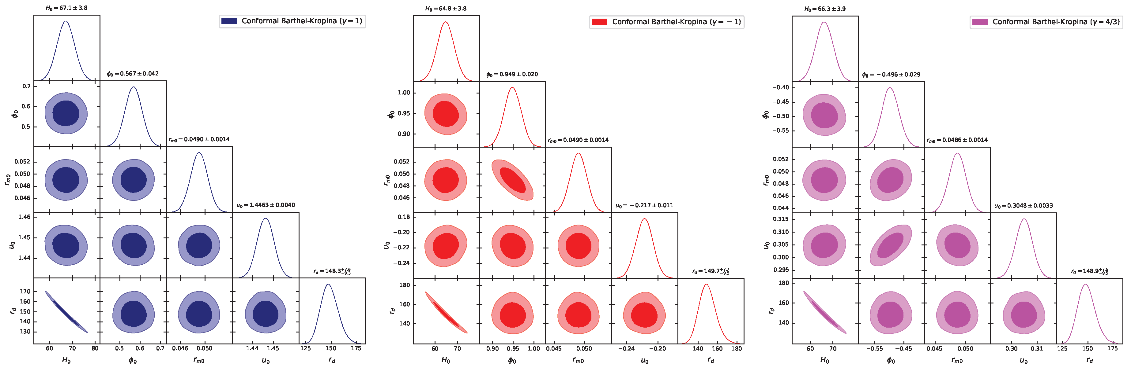
Figure 2.
The figure shows a comparative analysis of the Conformal Barthel–Kropina model for , , and against the CDM model and the CC measurements, which are represented by blue dots with corresponding green error bars. The left panel shows the evolution of the Hubble function , while the right panel shows the evolution of the Hubble residual .
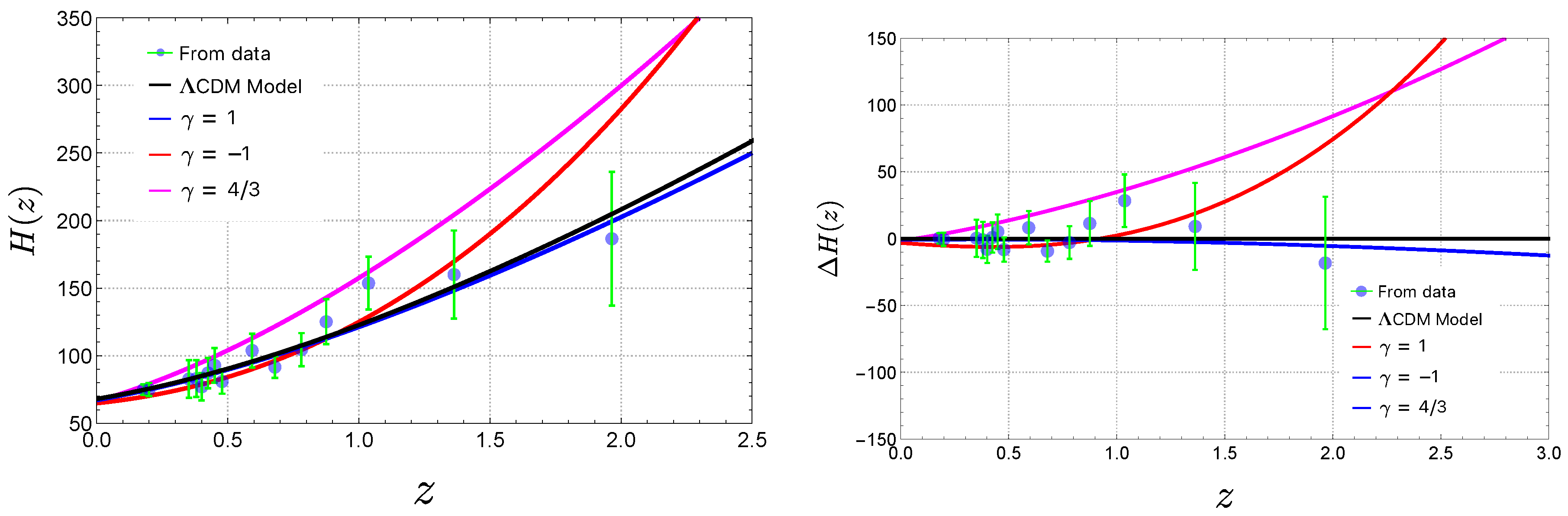
Figure 3.
The figure shows the evolution of the Conformal Barthel–Kropina model compared to the CDM model, with the deceleration parameter show in the left panel and the jerk parameter in the right panel for , , and .
Figure 3.
The figure shows the evolution of the Conformal Barthel–Kropina model compared to the CDM model, with the deceleration parameter show in the left panel and the jerk parameter in the right panel for , , and .
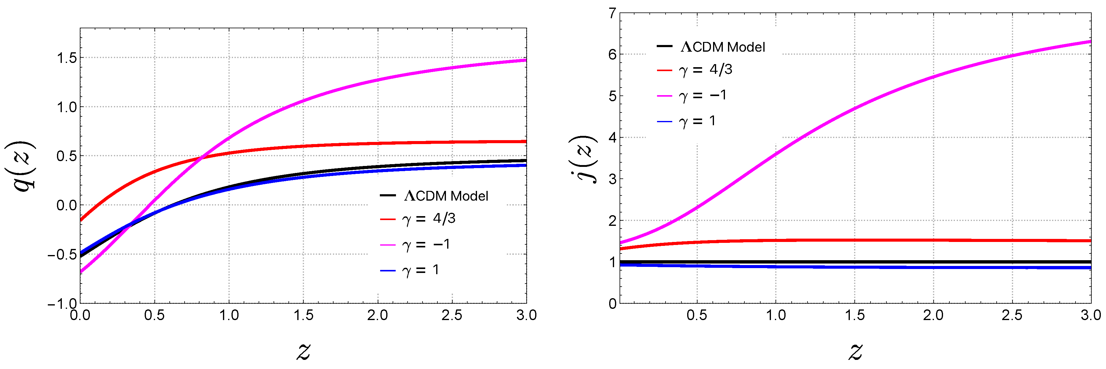
Figure 4.
The figure shows the evolution of the Conformal Barthel–Randers model compared to the CDM model, showing the dimensionless matter density on the left panel and the conformal factor on the right panel for , , and .
Figure 4.
The figure shows the evolution of the Conformal Barthel–Randers model compared to the CDM model, showing the dimensionless matter density on the left panel and the conformal factor on the right panel for , , and .
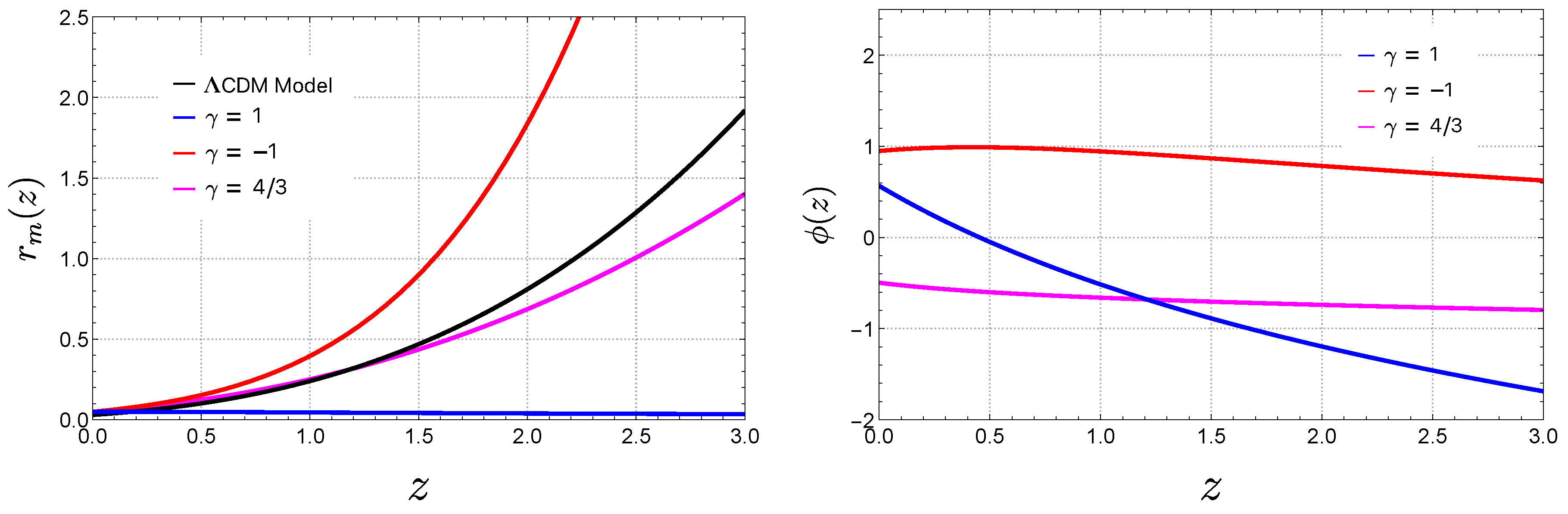

Table 1.
This table shows the numerical values of the parameters for the Conformal Barthel–Kropina cosmological models and the CDM model, showing mean values with 68% credible intervals (1) along with the corresponding priors.
Table 1.
This table shows the numerical values of the parameters for the Conformal Barthel–Kropina cosmological models and the CDM model, showing mean values with 68% credible intervals (1) along with the corresponding priors.
| Cosmological Models | Parameter | Prior | JOINT |
|---|---|---|---|
| CDM Model | |||
| Conformal | |||
| Barthel–Kropina () | |||
| Conformal | |||
| Barthel–Kropina () | |||
| Conformal | |||
| Barthel–Kropina () | |||
Table 2.
This table shows the statistical metrics for the CDM and Conformal Barthel–Kropina models, including , , AIC, AIC, BIC, BIC, p-value, and .
Table 2.
This table shows the statistical metrics for the CDM and Conformal Barthel–Kropina models, including , , AIC, AIC, BIC, BIC, p-value, and .
| Models | AIC | AIC | BIC | BIC | p-value | |||
|---|---|---|---|---|---|---|---|---|
| CDM | 1574.88 | 0.975 | 1597.04 | 0 | 1580.88 | 0 | 0.758 | 0 |
| CBR () | 1563.64 | 0.969 | 1573.64 | -23.40 | 1600.58 | 19.70 | 0.806 | 6.07 |
| CBR () | 1539.29 | 0.954 | 1549.29 | -47.75 | 1576.24 | -4.64 | 0.904 | 13.12 |
| CBR () | 1545.15 | 0.957 | 1555.15 | -41.89 | 1582.10 | 1.22 | 0.884 | 10.55 |
Disclaimer/Publisher’s Note: The statements, opinions and data contained in all publications are solely those of the individual author(s) and contributor(s) and not of MDPI and/or the editor(s). MDPI and/or the editor(s) disclaim responsibility for any injury to people or property resulting from any ideas, methods, instructions or products referred to in the content. |
© 2025 by the authors. Licensee MDPI, Basel, Switzerland. This article is an open access article distributed under the terms and conditions of the Creative Commons Attribution (CC BY) license (http://creativecommons.org/licenses/by/4.0/).
Copyright: This open access article is published under a Creative Commons CC BY 4.0 license, which permit the free download, distribution, and reuse, provided that the author and preprint are cited in any reuse.


