Submitted:
26 September 2025
Posted:
29 September 2025
You are already at the latest version
Abstract
This work introduces a block-coupled finite volume method for simulating the large-strain deformation of incompressible hyperelastic solids. Conventional displacement based finite volume solvers for incompressible materials often face stability and convergence challenges, particularly on unstructured meshes and in finite-strain regimes typical of biological tissues. To address these issues, a mixed displacement–pressure formulation is adopted and solved using a block-coupled strategy, enabling simultaneous solution of displacement and pressure increments. This eliminates the need for under-relaxation and improves robustness compared to segregated approaches. The method incorporates several enhancements, including temporally consistent Rhie–Chow interpolation, accurate treatment of traction boundary conditions, and compatibility with a wide range of constitutive models, from linear elasticity to advanced hyperelastic laws such as Holzapfel–Gasser–Ogden and Guccione. Implemented within the solids4Foam toolbox for OpenFOAM, the solver is validated against analytical and finite element benchmarks across diverse test cases, including uniaxial extension, simple shear, pressurized cylinders, arterial wall and idealised ventricle inflation. Results demonstrate second-order spatial and temporal accuracy, excellent agreement with reference solutions, and reliable performance in three-dimensional scenarios. The proposed approach establishes a robust foundation for fluid–structure interaction simulations in vascular and soft tissue biomechanics.
Keywords:
cell-centred finite volume method
; hyperelasticity
; incompressibility
; block-coupled
; solid mechanics
; soft tissue
; vascular mechanics
; OpenFOAM
; solids4Foam
1. Introduction
A considerable range of engineering applications involve materials capable of sustaining large-strain elastic deformations while exhibiting incompressible or nearly incompressible mechanical behavior. Rubber is a canonical example that is capable of undergoing substantial stretching or bending without an appreciable change in volume. Many soft biological tissues, including muscle, skin, and arterial walls, are commonly idealized as incompressible because of their high water content, which effectively suppresses volumetric change. Hydrogels and silicone gels exhibit similar characteristics, and many engineering elastomers (such as polyurethane and silicone rubber) are also modeled as incompressible in mechanical analyses.
It is well established that numerical stress analysis of solids approaching the incompressible limit presents significant challenges, particularly when a displacement-based formulation is employed. In particular, fully integrated, displacement-based lower-order finite elements often exhibit volumetric locking, a phenomenon frequently accompanied by pressure oscillations. Both volumetric locking and pressure oscillations have been extensively studied, leading to the development of various strategies aimed at mitigating these issues. The most widely used approach to prevent volumetric locking within the Finite Element (FE) framework is the mixed displacement-pressure formulation [1]. This method introduces pressure as an independent variable alongside displacement, allowing the problem to be formulated in a way that enforces the incompressibility constraint without locking.
In Computational Solid Mechanics (CSM), the FE method remains the most widely used approach. However, the Finite Volume (FV) method - long established in Computational Fluid Dynamics - has been steadily expanding its reach into CSM. Its growing popularity is due to its conceptual simplicity and strong conservation properties. Over the years, the FV method has been applied to a broad spectrum of CSM problems, emerging in several distinct variants based on different control volume arrangements, most notably cell-centred and vertex-centred schemes. A comprehensive review is provided in [2].
Only a limited number of FV methods have been proposed for incompressible bodies [3]. The present study builds on the work of Professor I. Demirdžić and collaborators [4,5,6], who employed a mixed displacement–pressure formulation to prevent volumetric locking. The mathematical model consists of the momentum equation, the mass conservation equation (incompressibility condition) and the constitutive equation. Spatial discretisation is performed using a cell-centred FV method applied to meshes with control volumes of completely arbitrary topology. The resulting set of coupled linear algebraic equations is solved using a segregated procedure incorporating a SIMPLE-based algorithm [7], which ensures the required pressure–displacement coupling through the use of Rhie–Chow interpolation [8] to evaluate displacement at the control volume faces. In the present study, the following improvements to the above models are proposed:
- Block-coupled solution procedure – Instead of using a segregated solution procedure, in which displacement increment components and the pressure increment are solved separately, a block-coupled system of linear algebraic equations (representing the discretised momentum and pressure increment equations) is solved for displacement and pressure increments simultaneously. This leads to a more robust and efficient solution process, as there is no need to apply user-defined under-relaxation to the displacement and pressure increments. The proposed block-coupled solution procedure is based on the procedure proposed by Professor M. Darwish and collaborators [9,10] for the solution of laminar incompressible flow problems on collocated unstructured FV grids. Later, a similar algorithm was implemented [11,12] in the OpenFOAM framework [13], which serves as the starting point for the implementation of an algorithm for solving incompressible elastic/hyperelastic solid deformations in this work.
- Temporal discretisation - Emphasis is placed on the temporal accuracy of the model, as the ultimate objective is its application to fluid–structure interaction simulations in vascular flows. Four commonly used temporal discretisation schemes are implemented and tested, each incorporating a temporally consistent Rhie–Chow interpolation [14].
- Improved treatment of traction boundaries - Along the portions of the discretized spatial domain boundary where traction is specified, the displacement increment is calculated using the cell-face normal component obtained from the solution of the continuity (pressure increment) equation, while the remaining components are reconstructed using the selected constitutive equation. This approach provides substantially higher accuracy at the traction boundaries compared to the second-order extrapolation used in [4].
- Extended material applicability – The proposed FV solver is applicable to both linear elastic bodies and nonlinear hyperelastic materials described by arbitrary constitutive equations, with emphasis on constitutive relations used for modeling arterial walls and heart tissue (for exampe, Holzapfel-Gasser-Ogden (HGO) model [15] and Guccione model [16]).
The proposed FV solver for incompressible elastic/hyperelastic bodies is implemented within the solids4Foam toolbox [17,18], which extends the OpenFOAM framework to allow the straightforward implementation of advanced solid mechanics and fluid–structure interaction (FSI) procedures. In this way, the proposed FV solver provides the foundation for developing a self-contained FSI solver for vascular flows in the next step.
In the next section, the governing equations and constitutive relations are presented, followed by a brief description of the FV discretisation procedure and the solution algorithm. Finally, the capabilities of the method are demonstrated through a series of test cases.
2. Mathematical Model
The deformation of an arbitrary body of volume , bounded by a surface , is governed by the law of conservation of linear momentum, which can be expressed in the following integral form:
where t is time, is density, is the displacement vector, is the outward-pointing normal vector of the surface , is the Cauchy stress tensor and the body force is omitted due to clarity. Equation (1) is integrated over the body in the deformed configuration. In this study, the alternative formulation of the linear momentum conservation law is used where integration is performed over the body in the initial undeformed configuration:
where the superscript 0 indicates that a quantity refers to the initial configuration (); for example, denotes the initial undeformed volume bounded by the corresponding initial undeformed surface . In the surface integral on the right-hand side of Equation (2), Nanson’s formula is used to transform the elementary area vector from the initial to the current configuration, where is the deformation gradient tensor, is the Jacobian of the deformation gradient, is the unit (identity) tensor, and denotes the gradient operator with respect to the initial configuration1. To close the model, it is necessary to specify the constitutive relation between the Cauchy stress tensor and the displacement vector , which is presented in the following section.
2.1. Constitutive Equations
The ultimate goal of this study is to develop a finite-volume solver for the simulation of large-strain dynamic deformation in elastic bodies composed of incompressible material, with a particular focus on applications in vascular system modelling. The solver currently handles incompressible elasticity/hyperelasticity but can be readily extended to compressible materials, following the same numerical approach as in [19]. Moreover, it consistently recovers the limit of linear elasticity, corresponding to small strains and rotations.
Constitutive relation for an isotropic linear elastic solid valid only under the small strain and small rotation assumption is Hook’s law:
where and are Láme coefficients and is the linear strain tensor:
The Láme coefficients and as well as the bulk elasticity modulus K can be defined through Young’s elasticity modulus E and Poisson’s ratio by the following relations:
It can be observed that Equation (3) is not well defined in the incompressible limit sice for , and . To avoid this issue, pressure can be introduced as an additional independent variable, defined by the following equation:
Taking into account Equation (6), Hook’s law (3) can be rewritten in a mixed (pressure-displacement) formulation as follows:
In the limit of incompressibility while and , hence Equations (7) and (8) reduce to
which represents well defined constitutive relation for incompressible linear elastic material. Equation (10) represents the continuity equation for an incompressible material and is also referred to as the incompressibility condition.
Nonlinear elastic behaviour can be represented by various hyperelastic models. Here, the Neo-Hookean law is used as a reference, and the solver is structured to easily incorporate alternative formulations.
Deformation of a compressible Neo-Hookean solid (Ogden variant) can be described with the following constitutive relation in the mixed (pressure-displacement) formulation:
where is the left Cauchy-Green tensor. A mixed formulation is again used in order to facilitate modelling of incompressible materials. In the limit of incompressibility Equation (11) reduces to:
The constitutive relations described above are expressed in terms of the total displacement , which is consistent with the total displacement formulation of the linear momentum conservation law (2). In this study, incremental displacement formulation of the linear momentum conservation law is applied since this approach can have positive effect on the efficiency and stability of an numerical procedure. Hance, it is necessary to express stress increment in terms of displacement increment , where superscript n refers to the known quantities from the previous time step2. Accordingly, one can express Cauchy stress increment tensor in terms of displacement increment and pressure increments for the incompressible Hook’s law as follows:
where is the pressure increment. Cauchy stress increment for incompressible Neo-Hookean solid reads as follows:
where the nonlinear quadratic term is omitted. One can note that expression (14) reduces to expression (13) if assumption of linear elasticity is satisfied ().
2.2. Resulting Set of Equations for Incompressible Solid
Resulting set of governing equation which are solved numerically consists of linear momentum conservation law and mass conservation law (incompressibility conditions). As is mentioned earlier, in order to enhance numerical efficiency, the incremental formulation of the conservation laws is used.
Incremental formulation of the conservation law for total linear momentum reads as follows:
By expressing the Cauchy stress increment in the above equation in terms of the unknown displacement increment and pressure increment via the incremental constitutive relation (14), the balance of linear momentum takes the following final form:
where the traction from the previous time instance and the traction increment are defined as follows:
Equation (16), with tractions defined by Equations (17) and (18), is not exact even for the Neo-Hookean model because, in its derivation, the current deformation gradient is approximated by that from the previous time step () and the quadratic term in the incremental constitutive relation (14) is neglected. In addition, the effective or instantaneous shear modulus is used in Equation (18) instead of the shear modulus of the Neo-Hookean model3. The procedure used to calculate aproximate value of instantaneous shear modulus is described in Appendix A. To compensate for these approximations, the following traction-correction term is added to the right-hand side of Equation (16):
where superscript * represents quantities obtained in the previous iteration of the iterative solution procedure4. In such a way, the Cauchy stress tensor is evaluated using selected hyperelastic constitutive model based on the values of the unknown displacement (displacement gradient) and pressure fields from the previous iteration. Taking into account traction correction term defined by Equation (19), final form of linear momentum equation reads as follows:
In the case of linear-elastic material, the traction correction term vanishes and Equations (17) and (18) simplifies by taking into account that .
In order to close the model which consist of two unknown fields (displacement increment and pressure increment) it is necessary to take into account Equation (10) transformed into incremental integral form:
where integration is performed over the volume of the body in the current (deformed) configuration. Equation (21) does not represent governing equation for pressure increment but additional constrain for displacement increment. The so called pressure increment equation will be derived later by combining discretised counterparts of Equations (20) and (21).
2.3. Initial and Boundary Conditions
To complete the mathematical model, initial and boundary conditions must be specified. For the numerical solution of transient problems, it is necessary to prescribe the displacement and velocity at the initial time and at all computational points of the spatial solution domain. Boundary conditions must be specified at all times along all spatial domain boundaries. The most common boundary conditions in solid mechanics are prescribed displacement (Dirichlet) and prescribed traction (Neumann). These conditions may be constant or time-dependent.
3. Numerical Model
The mathematical model is discretised in space using a second-order accurate collocated (cell-centered) unstructured FV method, while numerical integration in time is performed using various implicit schemes. The discretisation procedure is divided into two parts: discretisation of the solution domain and discretisation of the governing equations.
3.1. Solution Domain Discretization
The solution domain consist of temporal solution domain (ie. total solution time) and spatial solution domain. The total solution time is divided into a finite number of time steps , and the equations are solved in a time-marching manner. In the unstructured FV discretisation, the spatial solution domain is partitioned into a finite number of convex polyhedral control volumes (CVs) or cells, each bounded by convex polygonal faces. The cells do not overlap and completely fill the spatial domain. Figure 1 illustrates a simple polyhedral control volume around the computational point P located at its centroid, the face f, the face area , the unit normal vector to the face, and the centroid N of the neighbouring CV sharing the face f. In general case, the interpolation point does not coincide with the face centre point f and distance between them is defined by the skewness correction vector . The geometry of a CV is fully determined by the positions of its vertices.
3.2. Governing Equations Discretization
The second-order FV discretisation of an integral conservation equation transforms the surface integrals into sums of face integrals and approximates them and the volume integrals to the second-order accuracy by using the midpoint rule. Temporal discretisation is carried out by numerical integration of the governing equation in time from the old time instance to the new time instance .
3.2.1. Momentum Equation Discretisation
The spatially discretized momentum equation (20) for the control volume can be written as:
where the subscripts P and f denote the cell-centre and face-centre values, respectively, with the summation taken over all faces bounding cell P. In Equation (22), the first term on the right-hand side is treated implicitly after discretisation, whereas the last two terms are explicit and evaluated using displacement and pressure fields (or their increments) from the previous time step or iteration.
The traction increment in the implicit term on the right-hand side of Equation (22) is obtained by discretizing Equation (18) at the centers of internal faces as follows:
where the second and third terms on the right-hand side are obtained by decomposition of the gradient transpose term as follows:
where is the tangential gradient operator.
The face normal derivative of displacement increment in Equation (23) is discretized using the central scheme with non-orthogonal and skewness correction as follows (see Figure 1):
where , and . The first term on the right-hand side of Equation (25) is treated implicitly, while the correction term is treated explicitly. The discretisation scheme in Equation (25) is also applied to the face-normal derivative of the normal displacement increment, , where is replaced by its normal component, .
The face-centre value of the pressure increment in Equation (23) is calculated using linear interpolation of the neighbouring cell-centre values with the skewness correction:
where is the skewness correction vector between the cell-face interpolation point and the cell-face centre f, as illustrated in Figure 1. The linear interpolation procedure is then defined as follows:
here is the interpolation factor (see Figure 1), and obtained cell-face value corresponds to the value at the interpolation point , which coincides with the cell-face centre f for a mesh without skewness5. The skewness correction term in Equation (26) is treated explicitly, meaning it is evaluated using the pressure increment field obtained from the previous iteration.
Fully discretised momentum equation is obtained by numerical integration of Equation (22) over the time interval , where approximation of the time integrals is carried out using implicit two-level Euler scheme, Crank-Nicolson (trapezoidal) scheme and implicit three-level backward scheme. Backward and trapezoidal schemes are also combined to form so called composite scheme proposed by Bathe [20]. The fully discretized momentum equation obtained by applying the above listed temporal discretisation schemes reads as follows:
- Euler scheme
- Crank-Nicolson scheme
- backward scheme
- composite scheme [21]: a simplified version is implemented here, where the Crank-Nicolson and backward scheme are applied alternately.
In the above expressions, the velocity is introduced as an auxiliary variable, defined as the temporal derivative of the displacement, . The velocity at the current time step is subsequently expressed in terms of the displacement and its increment by employing the same temporal discretisation scheme.
The fully discretised momentum equation can now be written in the form of a linear algebraic equation, which for cell P takes the form:
where and denote the central (diagonal) and neighbour (off-diagonal) tensorial coefficients associated with the displacement increment field, while and denote the corresponding vectorial coefficients associated with the pressure increment field. The source vector on the right-hand side depends on the solution due to the explicit treatment of certain terms (e.g., traction, non-orthogonal, and skewness corrections). The central and neighbour coefficients in Equation (34) as well as the right-hand side vector are defined in Appendix B for the first-order implicit Euler scheme.
3.2.2. Discretised Pressure Equation
Discretised momentum equation represented by Equation (34) must be complemented by an additional system of algebraic equation for unknown cell-centre pressure increment field. In this study, it is applied approach usually used to numerically solve incompressible fluid flow by applying collocated (cell-centered) finite volume method, where discretised pressure equation is derived by combining discretised momentum and continuity equations using Rhie-Chow momentum interpolation procedure [8].
For cell P, the discrete form of the incompressibility condition (21) reads:
where the integration is performed on the cell faces mapped to the configuration at , which represents the intermediate state between the previous and current configurations and will hereafter be denoted by an m subscript or superscript, that is, . This approach yields the highest accuracy, as shown in [4]. Taking into account above introduced convention, simplified representation of the discrete form of the incompressibility condition now reads:
The cell-face volume increment in Equation (35) is calculated using the Rhie-Chow interpolation procedure [8] as follows:
where the interpolated cell-face displacement increment is corrected by a term proportional to the difference between the pressure increment derivative interpolated to the face and the derivative computed directly at the face. This correction acts as a low-pass filter to prevent pressure-displacement decoupling and suppress oscillations in the pressure increment field. The diagonal coefficient is scalar quantity and consists only contributions from the temporal and normal derivative term in the discretised momentum equation [first two therms at the right-hand side of Equation (A1)]6. Following the block-coupled solution procedure proposed for incompressible fluid flow in [9], only the interpolated gradient of pressure increment term is treated explicitly after discretisation, while the two reminding terms are implicit. The cell-face derivative of pressure increment in Equation (37) is discretised using central differencing formula:
where is the unit vector along the line (see Figure 1). Here, it should be noted that the pressure derivative is taken along the line connecting two neighbouring cell centers instead along cell-face normal direction. According to [14], this simplification does not violate the efficiency of the low-pass filter.
Rhie-Chow momentum-weighted interpolation is widely used to prevent pressure-velocity decoupling in simulations of incompressible flow on meshes with a collocated variable arrangement. The original Rhie-Chow interpolation [8] was proposed for steady-state fluid flow simulations, and its direct application to transient problems can result in temporally inconsistent behaviour. Various modifications to the original formulation have been proposed for transient problems (see, for example, [22] and the comprehensive review in [14]). Here, we propose a temporally consistent Rhie-Chow interpolation that can be applied to transient simulations of incompressible solid deformation described by the governing equations in the pressure-displacement formulation. The modification is implemented through an explicit correction term in Equation (37), which is provided for first-order accurate implicit Euler temporal discretisation schemes in Appendix C.
Using Equation (37), the discretised incopressiblity condition (35) can be transformed into a discretised pressure increment equation, which can be expressed as a linear algebraic equation for the pressure increment of any cell P:
where and are diagonal and off-diagonal scalar coefficients related to the unknown pressure increment field, and are diagonal and off-diagonal vectorial coefficients related to the unknown displacement increment field and is the right-hand side of linear equation. The central and neighbour coefficients in Equation (39) as well as the right-hand side term are defined in Appendix B.
As will be shown later, Equations (34) and (39) are used to assemble block linear system which is solved for cell-centre displacement increment and cell-centre pressure increment . After cell-centre unknowns are obtained, Rhie-Chow interpolation formula (37) is used to calculate cell-face volume increment (volume sweep by the cell-faces), which is after that used to calculate "conservative" cell-face displacement increment as follows:
In this way, the calculated displacement increment is guaranteed to satisfy the discrete incompressibility condition (35).
3.2.3. Calculation of Gradients
The very important component of the solution procedure is the calculation of gradients of unknown fields. Pressure increment gradient is required at cell-centres, while displacement increment gradient has to be calculated at the cell-centres as well as at the cell-face centres. The cell-centre gradient of all fields is calculated using the least-squares linear fit [23]. This method produces a second-order accurate gradient irrespective of local mesh quality.
The face-centre gradient of displacement increment is used to evaluate explicit part at the right hand side of Equation (22). Full cell-centre gradient is composed from normal and tangential component as follows:
where the normal derivative of displacement increment is calculated using Equation (25), while tangential face-centre gradient is calculated by taking tangential component of interpolated cell-centre gradient:
where is the cell-face unit normal vector. The tangential gradient at the boundary cell face is evaluated by second-order accurate linear extrapolation of the neighbouring cell-centre gradients.
3.2.4. Mesh Vertices Displacement
Before the pressure-increment equation is discretized, the mesh is moved to an intermediate configuration by updating the positions of the vertices from their reference locations to the intermediate ones. The corresponding vertex displacements are reconstructed from the cell-center displacements of the surrounding cells using a weighted least-squares method with a linear fitting function (see details in [24]).
3.2.5. Initial and Boundary Condition
To start the transient simulation, it is necessary to specify the displacement and velocity at the initial time for all cell centres in the computational mesh. Boundary conditions must be applied to the cell faces that lie on the domain boundary.
Up to this point, the discretisation procedure has been described only for internal cell faces. To discretise the governing equations at boundary cell faces, it is necessary to take into account the specified boundary conditions. This is explained below for two typical boundary conditions: specified displacement increment (Dirichlet boundary condition) and specified traction (Neumann boundary condition).
If a specified displacement increment boundary condition is used, the normal derivative of the displacement increment in Equation (23) is approximated using the scheme defined by Equation (25), where is replaced by the specified boundary cell-face displacement increment . At the same boundary, zero normal-derivative boundary condition is applied for the pressure increment field, so that Equation (37) yields a boundary-face volume increment corresponding to the specified displacement increment. The zero normal-derivative boundary condition is also used to update the pressure increment at the corresponding boundary cell-face at the end of each outer iteration of the iterative solution procedure.
For boundary faces where specified traction increment boundary condition is applied, the traction increment term in Equation (22) is added to the source term (right hand side), and traction correction term is set to zero. At the same boundary faces, the specified pressure increment boundary conditions is applied, where pressure increment value is calculated from the constitutive equation using gradient of displacement increment at the boundary from the previous iteration. The cell-face displacement increment term in Equation (37) is defined implicitly at the boundary cell-face b as follows:
where is the displacement increment at the centre of the cell next to the considered boundary face b, is the normal distance between boundary face centre b and adjacent cell-centre P, the normal derivative of the displacement increment is defined as follows:
The superscript * denotes quantities obtained in the previous iteration, and the boundary face displacement increment is defined by Equation (40). In this equation, the tangential component of the displacement increment (first term on the right-hand side) is computed to satisfy the constitutive relation at traction-specified boundary faces.
3.2.6. Final Block-Coupled System of Linear Algebraic Equations
By combining the discretised momentum equation (34) with the discretised pressure-increment (incompressibility condition) equation (39), one obtains the following coupled system of algebraic equations for each cell P in the computational mesh:
where and are the dense matrices representing the diagonal and off-diagonal coefficients of the coupled linear system, obtained by combining the corresponding coefficients of the discretised momentum equation (34) and the discretised pressure equation (39), as is ilustrated for diagonal coefficient in Figure 2. For each cell P, it is defined the vector , which consists of the cell-centre unknown fields: the three components of the cell-centre displacement increment vector and the cell-centre pressure increment. For example, for cell P this vector of unknowns is given by . The vector on the right-hand side of Equation (45) is composed of the corresponding right-hand side vectors of the linear systems (34) and (39), as follows: . After composing the system of linear algebraic equations (45) for all cells in the computational mesh, the corresponding global linear system is obtained:
where is the square block matrix, is the block vector of unknown fields and is the block vector of the right-hand side, and their dimension is equal to the number of cells in the computational mesh. The block linear system (46) is solved using the Block-Jacobi preconditioner and the BiSGSTAB solver.
3.3. Solution Procedure
The overall solution procedure is summarized in Algorithm 1 and can be categorized as the fixed-point/Picard iteration method. The main part of the solution procedure is the outer iteration loop that starts with the assembly of the global linear system (46), where the elements of the vector in the current iteration (k) are calculated using the values of unknown fields obtained in the previous outer iteration (). The outer iteration loop repeats until the norm of the initial residual of the system (46) is greater than the predefined tolerance: .
| Algorithm 1 Block coupled solution procedure. |
|
4. Results
In this section, seven test cases are presented to demonstrate the solver’s performance across different deformation regimes. The infinite plate with a circular hole is first used to assess accuracy in the linear elastic regime. Next, uniaxial stretch and simple shear tests highlight the nonlinear capabilities of the solver under elementary deformation modes. Inflation of a pressurized cylinder illustrates both steady-state and transient behaviour, including temporal accuracy analysis for Euler, backward, trapezoidal, and composite discretisation schemes. The heart tissue beam test evaluates the solver’s accuracy and stability in transient problems involving large rotations and displacements. Solver performance with the HGO constitutive model is demonstrated through inflation of a rat carotid artery. Finally, ventricle inflation serves as a realistic three-dimensional benchmark. In all cases, results obtained with the FV method are compared with analytical or FE solutions obtained using FEBio software suit [25,26].
4.1. Infinite Plate with a Circular Hole Subjected to Uniform Tension
A plate with a circular hole in its centre is loaded with uniform tension in the axial direction (see Figure 3). The problem is considered as the plane strain. If the radius of the hole is small compared to the dimensions of the plate, then the analytical solution obtained for an infinitely large plate describes the stress and displacement distribution around the hole [27]:
where r and are polar coordinates, a is hole radius, is shear modulus, and is the Kolosov constant for plane strain deformation.
The plate material is assumed to be linear elastic, isotropic, and incompressible (Poisson’s ratio ), with Young’s modulus . Owing to the problem’s symmetry, only a quarter of the plate is modelled, as shown in Figure 4 (shaded area). Following earlier studies of the same problem, e.g., [19], the exact solution corresponding to is prescribed on all traction-specified boundaries (top and right dashed edges) to eliminate finite-domain effects.
Spatial accuracy is demonstrated by comparing results obtained using the proposed FV solver with the corresponding analytical solution. This comparison was first conducted for three meshes of similar resolution, each consisting of a different cell shape: quadrilateral, triangular, and polygonal7, as shown in Figure 4. Figure 5 presents a comparison of the x-component of the displacement vector and the -component of the stress tensor with analytical results along the boundary of the plate. Similarly, Figure 6 shows a comparison of the y-component of the displacement vector and the -component of the stress tensor along the boundary. Very good agreement is observed between the analytical solution and the FV solver results for all three cell shapes.
The order of spatial accuracy of the proposed FV solver is evaluated by performing simulations on four quadrilateral meshes with successively increasing numbers of cells (1000, 4000, 16,000, 64,000), with the coarsest mesh shown in Figure 4(a). The cell-centre errors are calculated for displacement magnitude and -component of the Cauchy stress in respect to the available analytical solution and magnitude of the errors are computed using standard norms (, , and ). Figure 7 presents the error norms as a function of the average cell size. Second-order accuracy is achieved for the displacement across all three norms, whereas for the -component of the Cauchy stress tensor, first-order accuracy is observed with respect to the norm, while second-order accuracy is attained for the remaining two norms.
4.2. Uniaxial Extension and Simple Shear Tests
To test the solvers’ nonlinear capabilities for fundamental types of deformation, an uniaxial extension test and a simple shear test are performed on a cube with dimensions . The cube is modeled as an incompressible material (). Both tests are solved using the Neo-Hookean and Guccione material laws. For the Neo-Hookean material, the shear modulus of the cube is . For the Guccione law, the material properties are , with . A detailed description of the incompressible Guccione constitutive relation is provided in Appendix D.2.
4.2.1. Uniaxial Extension Test
The simulation of uniaxial extension along the x-direction is performed on one quarter of the unit cube by applying symmetry boundary conditions on the - and -planes (see Figure 8). The -plane is also modeled as a symmetry plane to allow free contraction of the cube in the lateral directions. On the remaining boundaries, specified traction boundary conditions are applied, with the traction calculated from the available analytical solution. For uniaxial extension along the x-direction, the deformation gradient can be expressed in terms of the principal stretches as follows:
where for the case of an incompressible material. For a given deformation gradient, the Cauchy stress and the corresponding traction on the cube boundaries is calculated based on the selected constitutive relation. Simulations are performed for the principal stretch varying in the range 1–.
Figure 9 shows the deformed configuration of the cube for , calculated using the incompressible Neo-Hookean material. For the same material, Figure 10 presents a comparison between the numerical and analytical solutions for the stretches , the hydrostatic pressure, and the -component of the Cauchy stress. The numerical results closely follow the analytical solution. An analogous comparison for the incompressible Guccione material is shown in Figure 11.
4.2.2. Simple Shear Test
The simple shear test involves a deformation in which parallel planes of the material slide past each other. The deformation gradient for simple shear in the -plane is defined as
where is the shear strain. In this study, a simple shear deformation is applied to the unit cube shown in Figure 12. A zero-displacement boundary condition is imposed on the bottom surface, while fixed traction boundary conditions are applied on the remaining surfaces, with the traction calculated using the selected constitutive relation (Neo-Hookean or Guccione) and the deformation gradient defined in Equation 48. The shear strain is varied in the range 0–.
The reference and final (deformed) configurations of the cube are shown in Figure 13 for the Neo-Hookean material model and for . The current configuration is coloured by the displacement field, where one can note parallel and horizontal contour lines as is expected for the case considered. Figure 14 presents a comparison between the exact and numerically calculated displacement of the top surface of the cube for the Neo-Hookean and Guccione material models as a function of the specified shear strain , where the exact value of the displacement for the unit cube is .
4.3. Inflation of a Thick-Wall Cylinder
An infinitely long thick-walled cylinder with inner radius and outer radius , is subjected to pressure . This case was also solved in [4]. A plane strain deformation is assumed. The material of the cylinder is assumed to be incompressible and hyperelastic with Young’s modulus . The behaviour of the incompressible hyperelastic material is described by the Neo-Hookean constitutive relation.
Exploiting the geometric and loading symmetry, only one quarter of the domain is modeled, as shown in Figure 15, with symmetry boundary conditions applied on the corresponding planes. The outer wall is modeled as traction-free. The analytical solution for this problem is provided in Appendix A.
Figure 16 shows a hexahedral mesh with 65 cells and a polyhedral mesh with 1,338 cells. These meshes, together with two finer hexahedral meshes consisting of 260 and 1,040 cells, were used to compute the solution for an internal pressure of . The predicted radial displacement, radial stress, hoop stress, and pressure along the radius are compared to the analytical solution in Figure 17. The solutions obtained on the hexahedral meshes converge consistently to the analytical solution with increasing mesh resolution, and good agreement is also observed for the solution obtained on the polyhedral mesh. Temporal accuracy analysis, presented in continuation, is performed for results obtained on the finer hexahedral mesh.
To assess temporal accuracy, the case was solved using different time-step sizes: , , , , and . The prescribed pressure at the inner surface is increased linearly from to over a time period . The accuracy analysis is carried out at the time instance . The cell-centre displacement error is computed for solution obtained with the five largest time-step sizes with respect to the reference solution obtained with the smallest time-step size . The magnitude of the cell-centre displacement error was quantified using the norm.
The temporal accuracy is assessed for both linear and non-linear deformation regimes employing four temporal discretisation schemes: Euler, backward, Crank–Nicolson and composite. The corresponding displacement error norms are presented in Figure 18 as functions of the time-step size. For both deformation regimes, the Euler scheme exhibits the expected first-order convergence of the error, whereas the remaining schemes attain the expected second-order convergence.
Finally, the long-term temporal response of the cylinder was analysed for the case in which the internal pressure was first increased linearly from to over the interval to , and then decreased linearly back to over the interval to . For this scenario, the total energy of the isolated system must remain constant for , in the absence of external forcing. Figure 19 shows temporal response of kinetic, potential and total energy obtained using backward temporal discretisation scheme, where the total energy is computed as a sum of kinetic and potential energy and potential energy is calculated according to Neo-Hookean constitutive relation. One can note, expected behaviour of the total energy after time instance . Other second-order temporal discretisation schemes shows similar behaviour.
4.4. Heart Tissue Beam
In this benchmark test case proposed by Land et. al [28], one considers deformation of a thick beam of length, and quadratic cross section (see Figure 21). The test case is analysed for two hyperelastic constitutive models: incompressible Guccione model as originally proposed in [28] (fibre direction along long axis, constitutive parameters: , , , ) and incompressible Neo-Hookean model with shear modulus . The properties of the incompressible Guccione model approximately correspond to the heart tissue properties.
In first step, a mesh sensitivity study is performed where steady-state FV solution is compared with the corresponding solution obtained using FEBio software suit [25,26], verified on selected test cases proposed in [28]. The beam is discretised by a uniform structured mesh, and it is subjected to a uniform pressure load of on the bottom side, while the left side is fixed in all directions. Figure 21 shows the z-coordinate of the tip point A (defined in Figure 20) as a function of cell dimension, where one can note consistent convergence toward the FE benchmark solution. Figure 21 shows the maximal deflection of the beam. Results are given for a computational mesh.
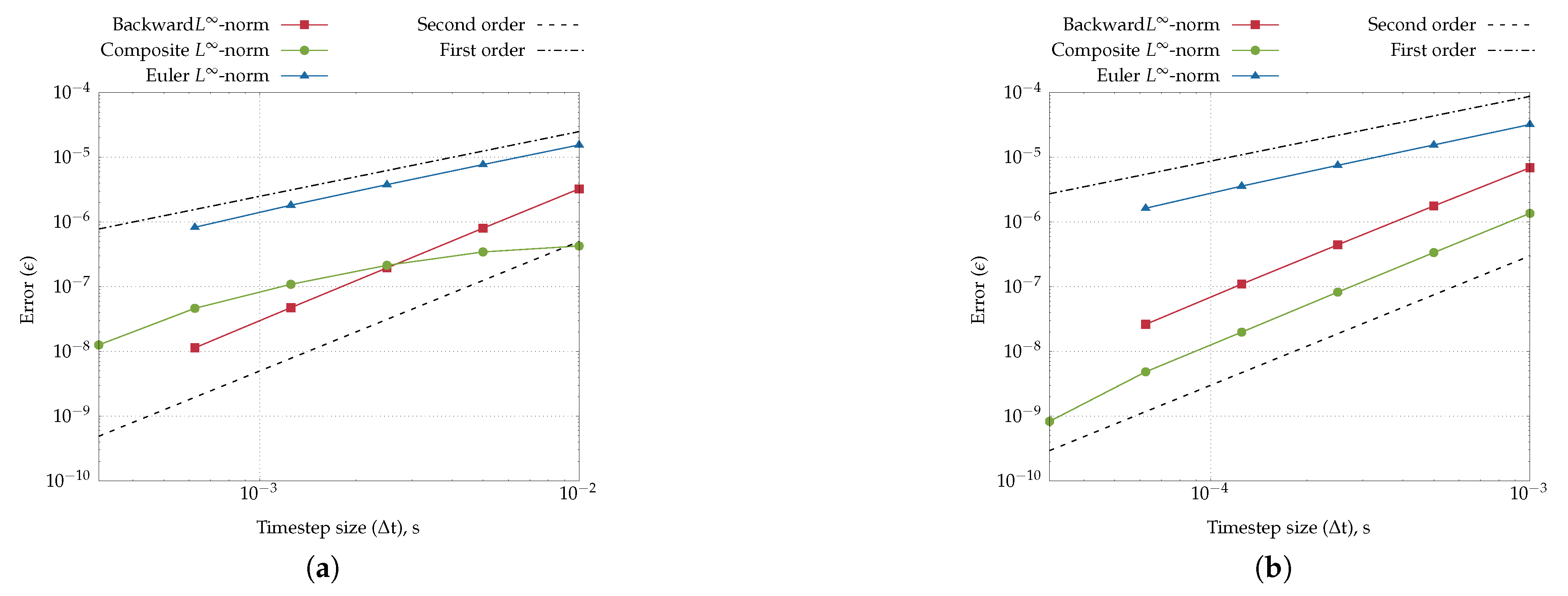
A temporal accuracy study was performed with the Neo-Hookean model, following the procedure outlined in Section 4.3. The results confirm first- and second-order accuracy for the Euler and backward time discretization schemes, respectively, as illustrated in Figure 22, for both linear and nonlinear models. Results obtained with the trapezoidal scheme are not reported, as numerical instabilities were observed for the smallest time-step sizes. To address this issue in nonlinear cases, the composite scheme proposed by Bathe and Noh [21] was employed. For sufficiently small time-step sizes, the composite scheme proposed by Bathe and Noh [21] attains second-order accuracy for both linear and nonlinear model.
Figure 20.
Heart tissue beam: reference configuration, with point A indicated.
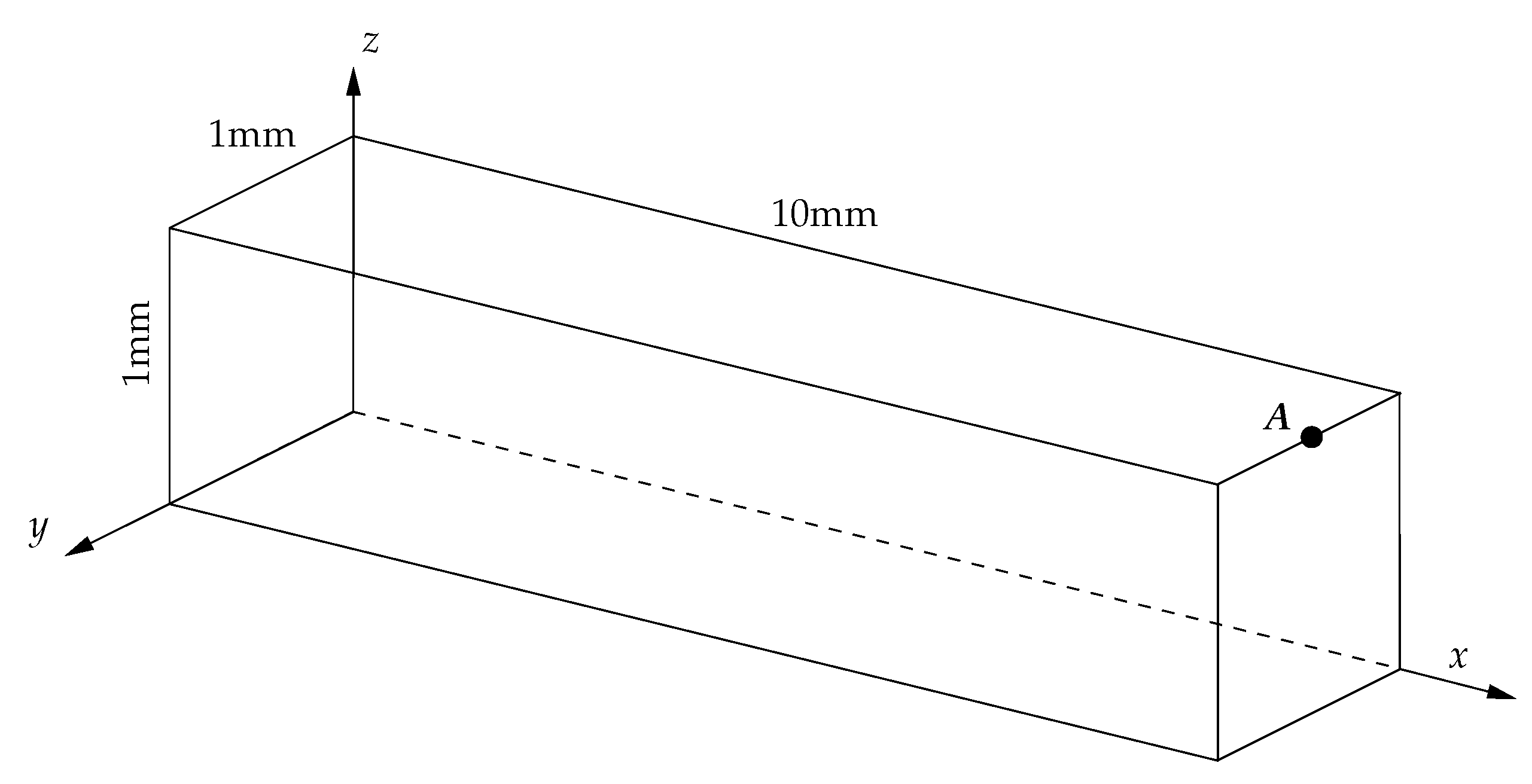
Figure 21.
Heart tissue beam: the computational mesh () in deformed configuration. Colors represent z-component of the displacement vector obtained for the Neo-Hookean material law.
Figure 21.
Heart tissue beam: the computational mesh () in deformed configuration. Colors represent z-component of the displacement vector obtained for the Neo-Hookean material law.
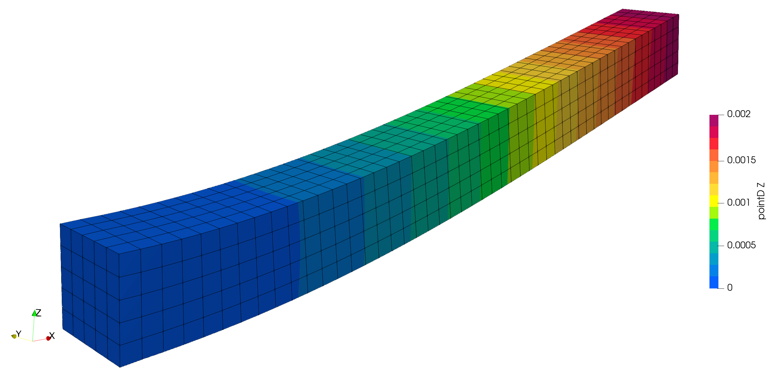
Figure 22.
Heart tissue beam: Time convergence study of the displacements for Euler and backward temporal schemes for (a) non-linear and (b) linear solver.
Figure 22.
Heart tissue beam: Time convergence study of the displacements for Euler and backward temporal schemes for (a) non-linear and (b) linear solver.
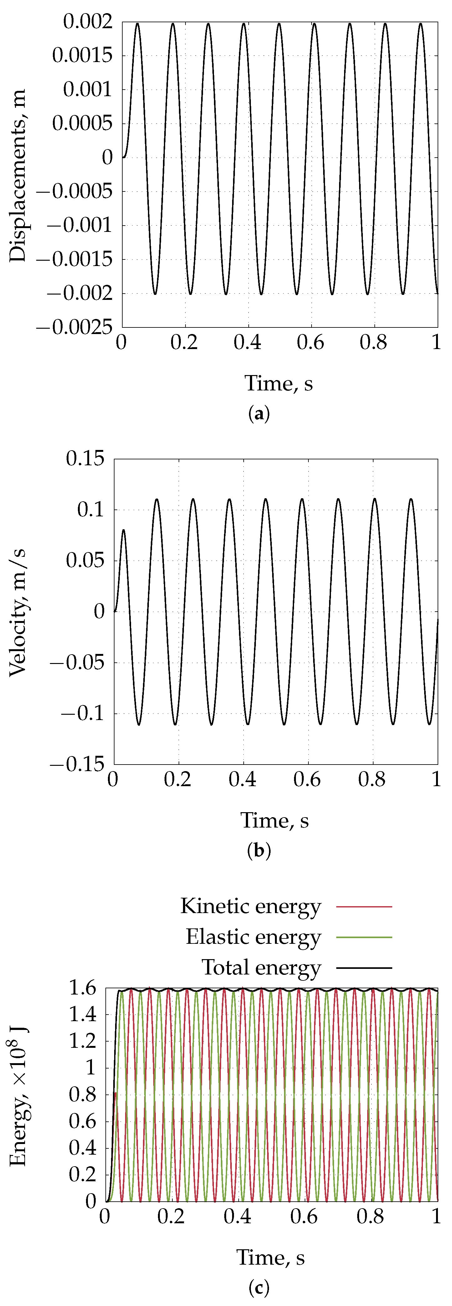
To check the stability of the solver for the long-term temporal response of the beam. The pressure, which is applied to the bottom side, is linearly increased to the maximum value of until , and then it is decreased back to until . Figure 24 and Figure 25 show the displacement and velocity of the tip of the beam, along with the kinetic, elastic, and total energy of the system, calculated using the Euler, backward, composite, and trapezoidal temporal schemes. Euler discretization scheme does not conserve the energy of the isolated system. In contrast, total energy remains constant after the force is no longer applied when using backward, Crank-Nicolson, and composite temporal discretisation schemes.
Figure 23.
Heart tissue beam: Error in maximal z-deflection at beam tip for different mesh densities for Neo-Hookean material law. Results converge to a consensus solution as the number of volumes increases.
Figure 23.
Heart tissue beam: Error in maximal z-deflection at beam tip for different mesh densities for Neo-Hookean material law. Results converge to a consensus solution as the number of volumes increases.
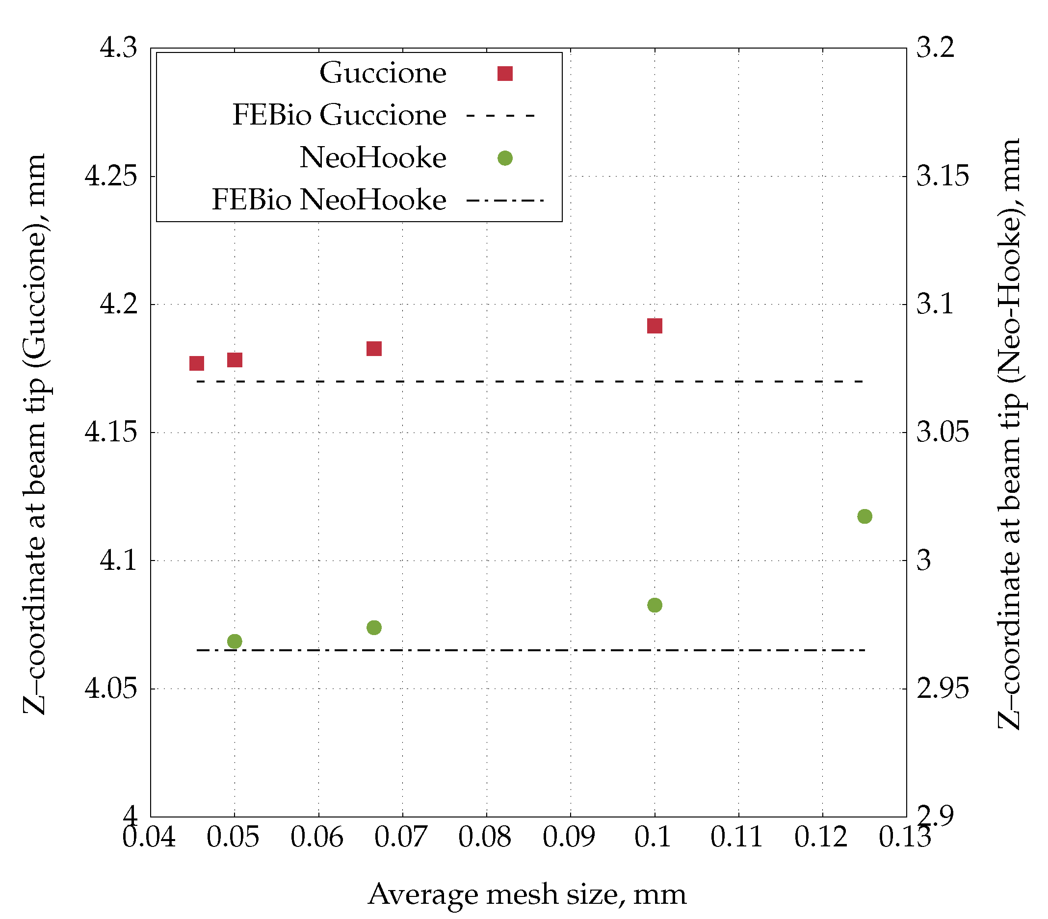
Figure 24.
Heart tissue beam: Displacements, velocity, and energy of the system with Euler temporal discretization.
Figure 24.
Heart tissue beam: Displacements, velocity, and energy of the system with Euler temporal discretization.
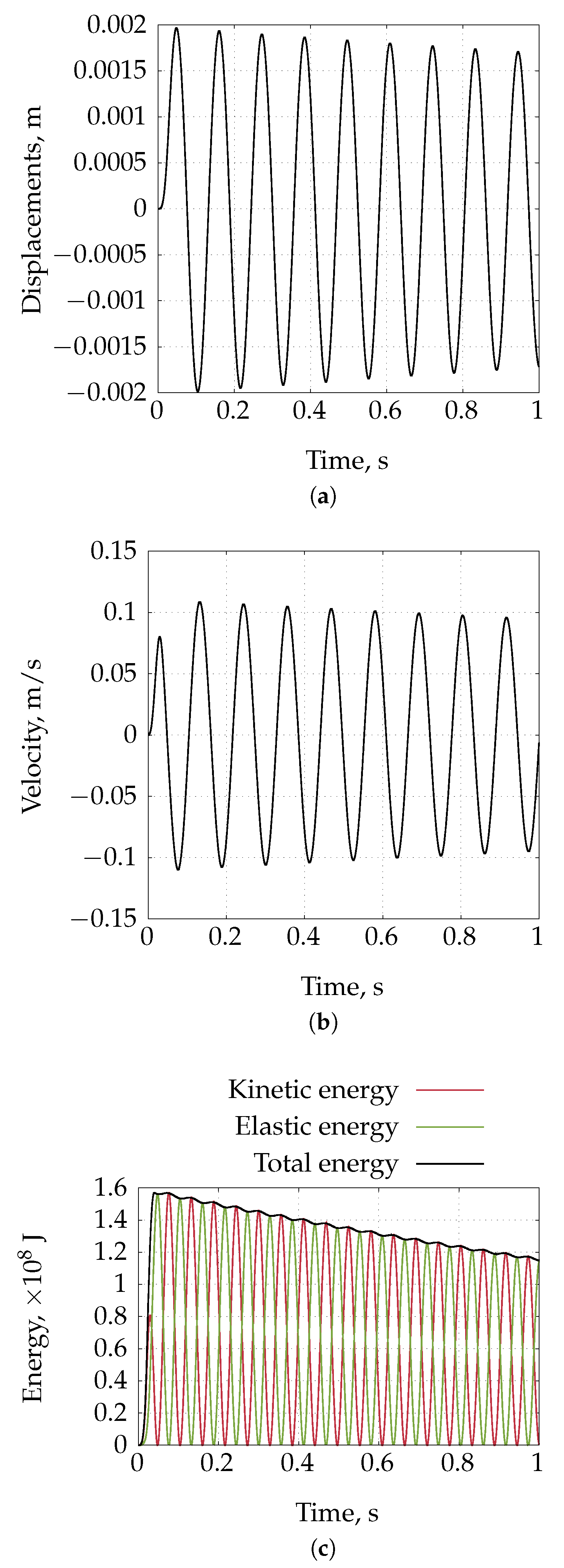
Figure 25.
Heart tissue beam: Displacements, velocity, and energy of the system with backward temporal discretization.
Figure 25.
Heart tissue beam: Displacements, velocity, and energy of the system with backward temporal discretization.
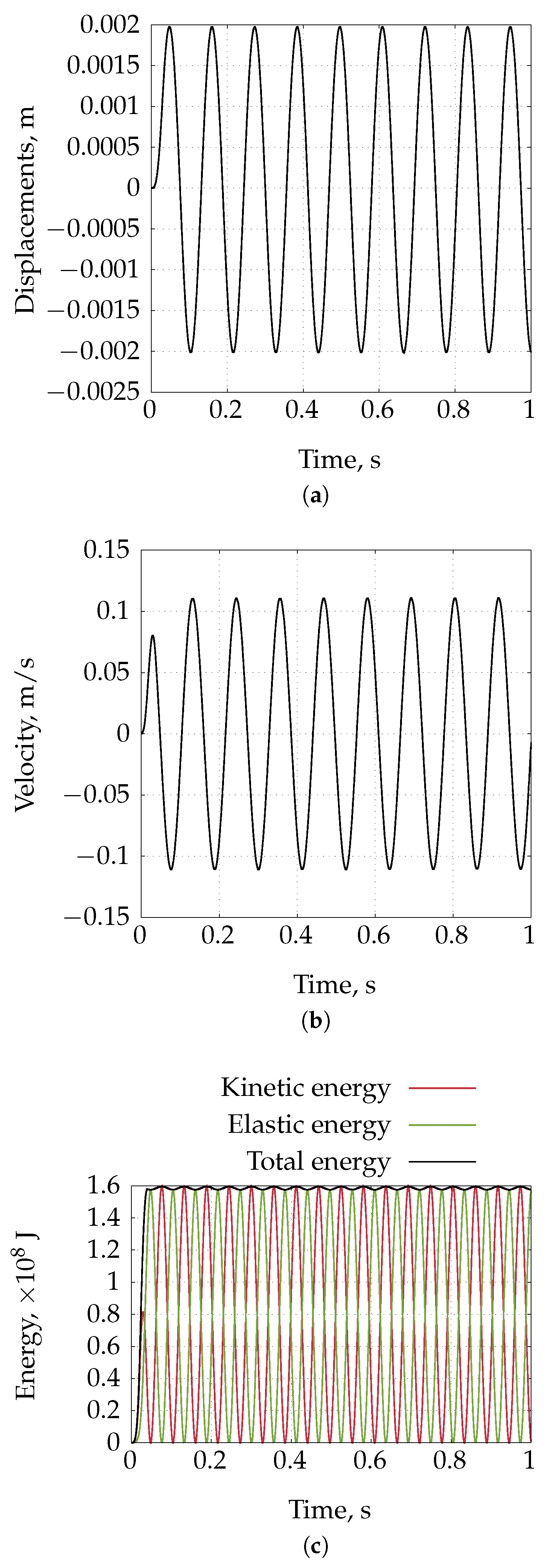
Figure 26.
Heart tissue beam: Displacements, velocity, and energy of the system with composite temporal discretization.
Figure 26.
Heart tissue beam: Displacements, velocity, and energy of the system with composite temporal discretization.
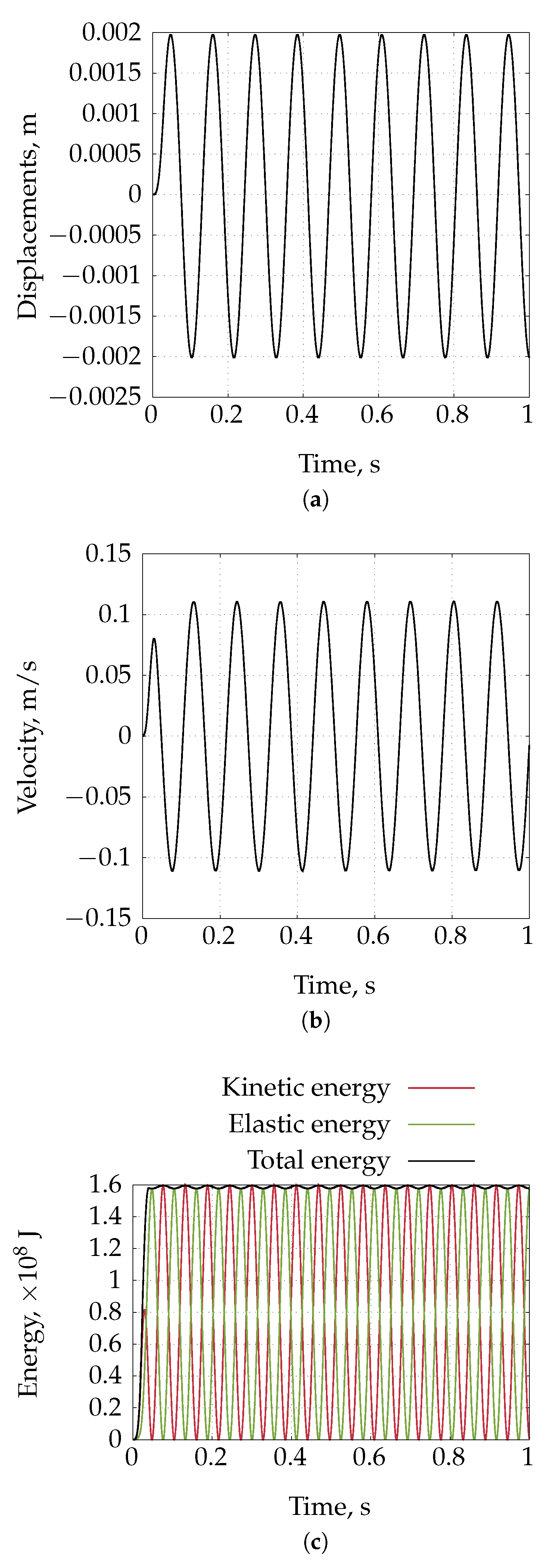
Figure 27.
Heart tissue beam: Displacements, velocity, and energy of the system with trapezoidal temporal discretization.
Figure 27.
Heart tissue beam: Displacements, velocity, and energy of the system with trapezoidal temporal discretization.
4.5. Inflation of a Rat Carotid Artery
This test case is based on the experimental study reported in [29], where carotid arteries were harvested from rats and subjected to internal pressurization, during which the outer radius was measured as a function of the applied pressure. Based on these experimental data, the HGO material model [15] was calibrated in [30]. This constitutive model effectively captures the anisotropic mechanical response of arterial walls by decomposing the strain energy density function into two components: an isotropic part, dominant at low pressures and consistent with a Neo-Hookean material behavior, and an anisotropic part, which becomes prominent at higher pressures which models the effect of progressive straightening of helically oriented collagen fibres. The material parameters were defined as follows [30]: Young’s modulus , , and . The collagen fibers were assumed to be symmetrically oriented at with respect to the circumferential direction.
In this study, numerical simulations of the rat carotid artery inflation, as described above, are performed following a similar FE study by Sun et al. [31]. The computational domain is defined as a cylindrical segment with an inner radius of , an outer radius of , and a length of . Axial displacements are constrained. Owing to geometric and loading symmetry, only one quarter of the domain is modeled, as illustrated in Figure 28, with appropriate symmetry boundary conditions applied on the corresponding planes. The outer wall is assumed to be traction-free, while an internal pressure of is applied to the inner wall through 100 loading steps.
Figure 28 also shows the deformed geometry at the final loading step. The evolution of the inner and outer radii of the cylindrical surfaces as a function of the applied inner pressure, obtained with the FV solver, is presented in Figure 29. Results for the inner surface are compared with experimental data from [29] and FE results from [31], while results for the outer surface are compared against FE results only. Overall, good agreement is observed.
4.6. Inflation of an Idealised Ventricle
Inflation of an idealised ventricle (Figure 30) was proposed by Land et al. [28] as a benchmark problem for cardiac mechanics software. The case is three-dimensional and static, with finite hyperelastic deformation. The initial geometry is defined as a truncated ellipsoid:
The endocardial (inner) surface is defined as , , , and . The epicardial (outer) surface is defined as , , , and . The implicitly defined base plane is positioned at . The behavior of hyperelastic material is described by the transversely isotropic incompressible Guccione model [16], where the parameters are , (the specified parameters produce isotropic behavior).
Although the geometry is axisymmetric, one quarter of the domain is modeled, as shown in Figure 30. The geometry is discretized entirely with hexahedral prisms. The epicardial surface is modelled as traction-free, while a fixed displacement boundary condition is prescribed on the top base plane. Symmetry boundary conditions are applied to the two cutting planes used to extract the quarter section of the ventricle. The endocardial surface is subjected to an internal pressure of . The internal pressure value of proposed in [28] could not be reached with the proposed FV solver due to the occurrence of unphysical pressure oscillations.
The load is applied incrementally in steps of . Simulations are performed on three successively refined meshes containing 2728, 16992, and 38292 cells. The reference solution is obtained using the FEBio software on the finest mesh. Figure 31 shows the magnitude of the apex displacement at the endocardial and epicardial surfaces as a function of the pressure load applied to the endocardial surface. The solution obtained using the proposed FV solver consistently converges with mesh refinement toward the reference FE solution. Figure 32 shows a comparison of the ventricle shape at loading pressure of . Figure 32a shows ventricle wall midline in its undeformed and deformed configurations obtained using FV and FEBio solvers. Similarly, Figure 32b shows undeformed and deformed configuration for a line on the endocardial surface. In both cases one can observe very good agreement between FV and FE results.
The simulations described above (performed using incompressible Guccione constitutive model) were repeated with the incompressible Neo-Hookean constitutive model, with the shear modulus set to , corresponding to the initial shear modulus of the Guccione model. The maximum achievable pressure load on the endocardial surface was for both the proposed FV solver and the FE solver. The remaining boundary conditions were identical to those described previously.
Figure 33 illustrates the apex displacement magnitude at the endocardial and epicardial surfaces as a function of the applied internal pressure load, showing convergence toward the reference results with mesh refinement. Figure 34 compares the overall ventricle shape at an internal pressure of , as computed with the proposed FV solver and the FEBio tool. Figure 34a presents the deformed configuration of the ventricle wall midline, while Figure 34b examines the deformed shape of a line on the endocardial surface. In both cases, the FV and FE results demonstrate very good agreement.
Acknowledgments
This work was supported by grants from the Croatian Science Foundation (projects IP-2020-02-4016 and DOK-2021-02-3071, PI: Ž Tuković; projects IP-2018-01-3796 and DOK-2020-01-5698, PIs: D. Ozretić and I. Karšaj).
Abbreviations
The following abbreviations are used in this manuscript:
| FE | Finite Element |
| CSM | Computational Solid Mechanics |
| FV | Finite Volume |
| SIMPLE | Semi-Implicit Method for Pressure Linked Equations |
| FSI | Fluid-structure interaction |
| CV | Control volume |
| HGO | Holzapfel-Gasser-Ogden |
| CRC | Consistent Rhie-Chow |
Appendix A Instantaneous Shear Modulus Approximation
The instantaneous (effective) shear modulus, , is introduced in Equation (18) to account for the fact that the shear modulus generally changes during the deformation of a hyperelastic body. In the case of the Neo-Hookean constitutive model, the instantaneous shear modulus is constant and equal to the standard shear modulus . For other hyperelastic constitutive relations, the instantaneous shear modulus is approximated using the procedure described below.
The approximated value of the instantaneous shear modulus is calculated by numerically performing a simple shear test in three mutually perpendicular planes at the cell centers, taking into account the current state of deformation. In this way, three different values of the shear modulus are obtained, and the maximum value is taken as the effective shear modulus.
The above-described procedure is performed at the end of every time step, and the obtained effective shear modulus is then used in the calculations of the following time step. It is important to note that the value of the effective shear modulus does not influence the final solution; it only affects the efficiency of the solution procedure (i.e., the number of iterations required to reach convergence).
Appendix B Linear System Coefficients
The discretized momentum equation for an arbitrary cell P is expressed by Equation (34), where the central (diagonal) and neighbour (off-diagonal) tensorial () coefficients associated with the unknown displacement increment field read as follows:
Corresponding vectorial () coefficients associated with the unknown pressure increment field read as follows:
Finally, right-hand side (source) vector in Equation (34) reads as follows:
The discretized incompressibility condition for an arbitrary cell P is expressed by Equation (39), where the central (diagonal) and neighbour (off-diagonal) scalar coefficients associated with the unknown pressure increment field read as follows:
The vectorial coefficients related to the unknown displacement increment field are:
while the right-hand side term reads:
where is the displacement increment gradient evaluated on the intermediate configuration corresponding to the time instance .
Appendix C Consistent Rhie-Chow Interpolation
In this work, the temporally consistent Rhie-Chow interpolation is achieved by adding an explicit correction term, , to the right-hand side of Equation (37). The derivation of this correction term follows the approach proposed in Bartholomew et al. [14], adjusted to the particular problem considered in this work. The final form of the correction term for the case of the Euler temporal discretisation scheme reads as follows:
where is the cell-face velocity obtained by linear interpolation with skewness correction of the cell-center velocity and is the cell-face velocity calculated by taking the temporal derivative of the conservative cell-face displacement. The same procedure is used to derive the correction therm for the remaining temporal discretisation schemes.
Appendix D Material Laws
Appendix D.1. HGO Model
The Holzapfel–Gasser–Ogden (HGO) constitutive model is widely used to describe the nonlinear mechanical response of arterial tissue. In this implementation, the model is formulated with three material parameters and uses two families of collagen fibers. The fibers are assumed to be arranged symmetrically around the circumferential axis at angles . They reinforce the isotropic matrix and make the tissue stiffer and highly anisotropic.
The strain energy density function is defined as
where is the shear modulus of the isotropic ground matrix, and are material parameters associated with the collagen fibers, and , , and are strain invariants.
The invariants are computed as
where is the right Cauchy–Green deformation tensor, and , are unit vectors in the reference configuration defining the preferred fiber directions.
The corresponding Cauchy stress tensor is obtained as:
Appendix D.2. Guccione Model
To describe the mechanical behavior of cardiac tissue, the Guccione constitutive model was implemented. This model takes into account the presence of collagen fibers, which reinforce the tissue matrix and contribute to its stiffness and strength. As a result, the tissue exhibits anisotropic behavior, specifically transverse isotropy, due to the directional alignment of fibers.
The strain energy density function is defined as:
where k is a material constant and Q is a scalar function representing the anisotropic response of the tissue, given by:
Here, , , and are material parameters, and , , , and are invariants of the Green-Lagrange strain tensor . The Green-Lagrange strain is computed from the deformation gradient as:
with the deformation gradient defined as:
Where is the displacement vector and is the reference configuration. The strain invariants are computed as follows:
where is a unit vector of reference fiber direction.
The second Piola–Kirchhoff stress tensor is then obtained by differentiating the strain energy density concerning :
The derivative of Q with respect to the Green-Lagrange strain is:
Appendix A Pressurized Cylinder Equations
The strain energy density for an incompressible neo-Hookean material is:
where is the shear modulus. From the strain energy density function Eq. (A22), the Cauchy stress from can be written as:
The loading case and the geometry of the cylinder are shown on (Figure 15) in the reference configuration in a -section view. Based on this, the current configuration coordinates can be defined with respect to the reference configuration ones:
where is the axial stretch of the cylinder. The deformation gradient tensor can then be written as:
hence, the stretches are:
but considering that the material is incompressible, that the radial stretch is:
By using Eqs. (A25), (A26) and (A27) the left Cauchy-Green tensor can be written as:
while the components of the Cauchy stress tensor from Eq. (A23) become:
The equilibrium equation is:
which, when combined with Eq. (A29), leaves only the radial component as the non-trivial solution:
with the following boundary conditions
where a and b are the inner and outer radii of the cylinder in the current configuration respectively. Similarly, A and B are the inner and outer radii of the cylinder in the reference configuration.
By integrating Eq. (A27) from the internal surface up to some radius:
the current and reference configuration radii can be written as functions of one another:
By using Eq. (A33) the stretches from Eq. (A26) can be rewritten as functions of the reference configuration radius:
By integrating Eq. (A31) from the internal to the external surface, the following is obtained:
and by using Eq. (A33), after some rearranging, this becomes:
For practical reasons, define the variable as:
Hence, by prescribing the inner radius in the current configuration and the axial stretch , the loading pressure can be computed from Eq. (A38), assuming that the reference geometry of the cylinder is known, i.e. A and B.
Usually, though, the loading pressure p is known, and the geometry in the current configuration needs to be computed. If the inner radius in the current configuration is known, then it is easy to compute various other values (e.g. the deformed outer radius and the stress distribution). Consequently, Eq. (A38) can be used to compute the deformed inner radius if the loading pressure is known.
Using Eq. (A38), define the function:
by solving Eq. (A39) for a given geometry, loading pressure and axial stretch, the deformed internal radius a is obtained. This can be done by employing any number of methods, for example Newton’s method, for which the derivative of is required:
The distribution of the radial component of the Cauchy stress can be obtained by integrating Eq. (A31) from the internal surface up to some arbitrary radius:
which, upon further integration and after some rearranging yields:
note that p in Eq. (A42) refers to the internal loading pressure. Also note that by using Eq. (A33), Eq. (A42) can be expressed in terms of the reference configuration radius.
References
- Sussman, T.; Bathe, K.J. A finite element formulation for nonlinear incompressible elastic and inelastic analysis. Computers and Structures 1987, 26, 357–409. [Google Scholar] [CrossRef]
- Cardiff, P.; Demirdžić, I. Thirty Years of the Finite Volume Method for Solid Mechanics. Archives of Computational Methods in Engineering 2021, 28, 3721–3780. [Google Scholar] [CrossRef]
- Wheel, M.A. A mixed finite volume formulation for determining the small strain deformation of incompressible materials. International Journal for Numerical Methods in Engineering 1999, 44, 1843–1861. [Google Scholar] [CrossRef]
- Bijelonja, I.; Demirdžić, I.; Muzaferija, S. A finite volume method for large strain analysis of incompressible hyperelastic materials. International Journal for Numerical Methods in Engineering 2005, 64, 1594–1609. [Google Scholar] [CrossRef]
- Bijelonja, I.; Demirdžić, I.; Muzaferija, S. A finite volume method for incompressible linear elasticity. Computer Methods in Applied Mechanics and Engineering 2006, 195, 6378–6390. [Google Scholar] [CrossRef]
- Bijelonja, I.; Demirdžić, I.; Muzaferija, S. Mixed finite volume method for linear thermoelasticity at all Poisson’s ratios. Numerical Heat Transfer, Part A: Applications 2017, 72, 215–235. [Google Scholar] [CrossRef]
- Patankar, S.; Spalding, D. A calculation procedure for heat, mass and momentum transfer in three-dimensional parabolic flows. International Journal of Heat and Mass Transfer 1972, 15, 1787–1806. [Google Scholar] [CrossRef]
- Rhie, C.M.; Chow, W.L. Numerical study of the turbulent flow past an airfoil with trailing edge separation. AIAA Journal 1983, 21, 1525–1532. [Google Scholar] [CrossRef]
- Darwish, M.; Sraj, I.; Moukalled, F. A coupled finite volume solver for the solution of incompressible flows on unstructured grids. Journal of Computational Physics 2009, 228, 180–201. [Google Scholar] [CrossRef]
- Mangani, L.; Alloush, M.M.; Lindegger, R.; Hanimann, L.; Darwish, M. A Pressure-Based Fully-Coupled Flow Algorithm for the Control Volume Finite Element Method. Applied Sciences 2022, 12, 4633. [Google Scholar] [CrossRef]
- Uroić, T.; Jasak, H. Block-selective algebraic multigrid for implicitly coupled pressure-velocity system. Computers & Fluids 2018, 167, 100–110. [Google Scholar] [CrossRef]
- Fernandes, C.; Vukčević, V.; Uroić, T.; Simoes, R.; Carneiro, O.; Jasak, H.; Nóbrega, J. A coupled finite volume flow solver for the solution of incompressible viscoelastic flows. Journal of Non-Newtonian Fluid Mechanics 2019, 265, 99–115. [Google Scholar] [CrossRef]
- Weller, H.G.; Tabor, G.; Jasak, H.; Fureby, C. A tensorial approach to computational continuum mechanics using object-oriented techniques. Computers in Physics 1998, 12. [Google Scholar] [CrossRef]
- Bartholomew, P.; Denner, F.; Abdol-Azis, M.H.; Marquis, A.; van Wachem, B.G. Unified formulation of the momentum-weighted interpolation for collocated variable arrangements. Journal of Computational Physics 2018, 375, 177–208. [Google Scholar] [CrossRef]
- Holzapfel, G.A.; Gasser, T.C.; Ogden, R.W. A new constitutive framework for arterial wall mechanics and a comparative study of material models. Journal of Elasticity 2000, 61, 1–48. [Google Scholar] [CrossRef]
- Guccione, J.M.; McCulloch, A.D.; Waldman, L.K. Passive material properties of intact ventricular myocardium determined from a cylindrical model. Journal of Biomechanical Engineering 1991, 113, 42–55. [Google Scholar] [CrossRef]
- Cardiff, P.; Karač, A.; De Jaeger, P.; Jasak, H.; Nagy, J.; Ivanković, A.; Tuković, Ž. An open-source finite volume toolbox for solid mechanics and fluid-solid interaction simulations, 2018. [CrossRef]
- Cardiff, P.; Batistić, I.; Tuković, Ž. solids4foam: A toolbox for performing solid mechanics and fluid-solid interaction simulations in OpenFOAM. Journal of Open Source Software 2025, 10, 7407. [Google Scholar] [CrossRef]
- Demirdžić, I.; Cardiff, P. Symmetry plane boundary conditions for cell-centered finite-volume continuum mechanics. Numerical Heat Transfer, Part B: Fundamentals 2022, 83, 12–23. [Google Scholar] [CrossRef]
- Bathe, K.J.; Baig, M.M.I. On a composite implicit time integration procedure for nonlinear dynamics. Computers & Structures 2005, 83, 2513–2524. [Google Scholar] [CrossRef]
- Bathe, K.J.; Noh, G.C. On a composite implicit time integration procedure for nonlinear dynamics. Computers & Structures 2005, 83, 251–268. [Google Scholar] [CrossRef]
- Tuković, Ž.; Perić, M.; Jasak, H. Consistent second-order time-accurate non-iterative PISO-algorithm. Computers & Fluids 2018, 166, 78–85. [Google Scholar] [CrossRef]
- Demirdžić, I.; Muzaferija, S. Numerical method for coupled fluid flow, heat transfer and stress analysis using unstructured moving meshes with cells of arbitrary topology. Computer Methods in Applied Mechanics and Engineering 1995, 125, 235–255. [Google Scholar] [CrossRef]
- Tuković, Ž.; Karač, A.; Cardiff, P.; Jasak, H.; Ivanković, A. OpenFOAM Finite Volume Solver for Fluid-Solid Interaction. Transactions of FAMENA 2018, 42, 1–31. [Google Scholar] [CrossRef]
- Maas, S.A.; Ellis, B.J.; Ateshian, G.A.; Weiss, J.A. FEBio: Finite Elements for Biomechanics. Journal of Biomechanical Engineering 2012, 134. [Google Scholar] [CrossRef]
- Maas, S.A.; Ateshian, G.A.; Weiss, J.A. FEBio: History and Advances. Annual Review of Biomedical Engineering 2017, 19, 279–299. [Google Scholar] [CrossRef]
- Timoshenko, S.; Goodier, J. Theory of Elasticity; McGraw-Hill Book Company, 1970.
- Land, S.; Gurev, V.; Arens, S.; Augustin, C.M.; Baron, L.; Blake, R.; Bradley, C.; Castro, S.; Crozier, A.; Favino, M.; et al. Verification of cardiac mechanics software: benchmark problems and solutions for testing active and passive material behaviour. Proceedings of the Royal Society A: Mathematical, Physical and Engineering Sciences 2015, 471, 20150641. [Google Scholar] [CrossRef]
- P., F.; A., M.; H., M.; JJ., M.; K., H.; N., S. Short-Term biomechanical adaptation of the rat carotid to acute hypertension: contribution of smooth muscle. Annals of Biomedical Engineering 2001, 29, 26–34. 2001, 29, 26–34. [CrossRef]
- Zulliger, M.A.; Fridez, P.; Hayashi, K.; Stergiopulos, N. A strain energy function for arteries accounting for wall composition and structure. Journal of Biomechanics 2004, 37, 989–1000. [Google Scholar] [CrossRef]
- Sun, W.; Chaikof, E.L.; Levenston, M.E. Numerical Approximation of Tangent Moduli for Finite Element Implementations of Nonlinear Hyperelastic Material Models. Journal of Biomechanical Engineering 2008, 130, 061003. [Google Scholar] [CrossRef]
| 1 | When there is no difference between initial and current configuration like in the case of linear elasticity, subscript next to the ∇ operator is omitted. |
| 2 | Discretisation of temporal solution domain will be described later, but one can define here previous time instance , while current time instance is , where is the time-step size. |
| 3 | In the Neo-Hookean model, the shear modulus remains constant. In contrast, for example, in the HGO model the shear modulus coincides with that of the Neo-Hookean model in the undeformed state, but it evolves with deformation of the elastic body |
| 4 | It is usual practice to use iterative solution procedure to solve non-linear problems in computational mechanic. Even in the case of linear problems, iterative solution procedure have to be used in the framework of FV method since different kinds of corrections related to preservation of accuracy are applied using differed correction approach. |
| 5 | In the remainder of this manuscript, the operator denotes the calculation of cell-face values by linear interpolation of neighbouring cell-centre values without skewness correction, as defined in Equation (27), whereas the operator denotes the linear interpolation with skewness correction, as defined in Equation (26). Left-hand side superscript in the above operators indicates mesh configuration on which linear interpolation is performed and on which gradient for skewness correction is calculated. |
| 6 | The contribution arising from the normal derivative of the normal displacement increment is neglected, as it is tensorial in nature and would significantly increase the complexity of deriving the pressure increment equation. |
| 7 | In reality, the mesh is 3-D and consists of one layer of prismatic cells with quadrilateral, triangular and polygonal base. |
Figure 1.
An example of a polyhedral control volume (cell) P with its neighbour cell centre N and the shared face f.
Figure 1.
An example of a polyhedral control volume (cell) P with its neighbour cell centre N and the shared face f.
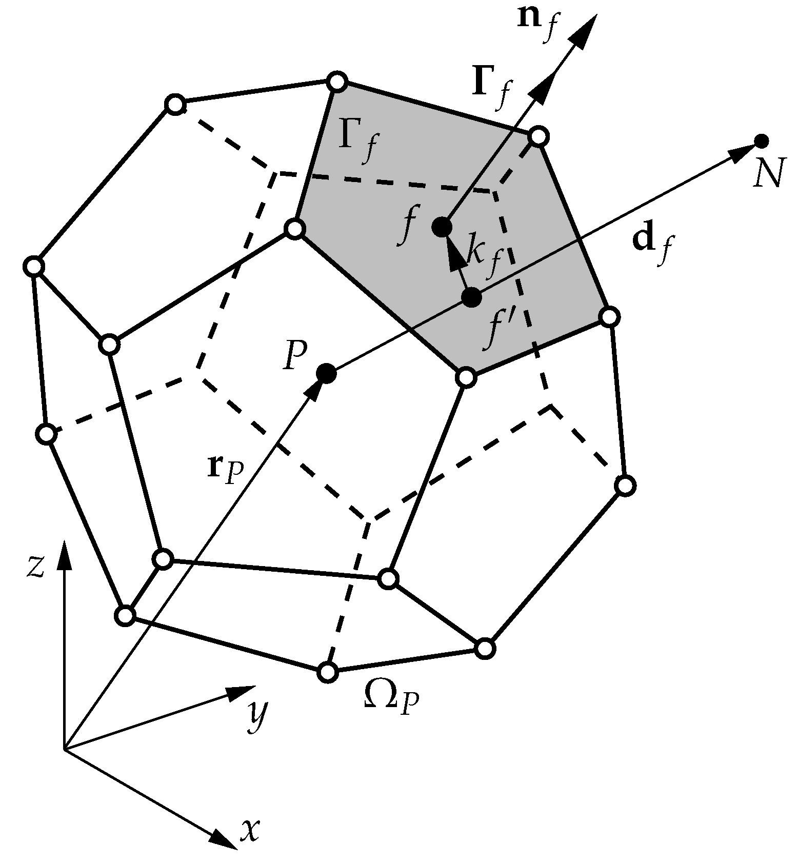
Figure 2.
Diagonal matrix coefficient of the block matrix at the node P, consisting of corresponding diagonal coefficients of the discretised linear momentum and pressure increment equations.
Figure 2.
Diagonal matrix coefficient of the block matrix at the node P, consisting of corresponding diagonal coefficients of the discretised linear momentum and pressure increment equations.
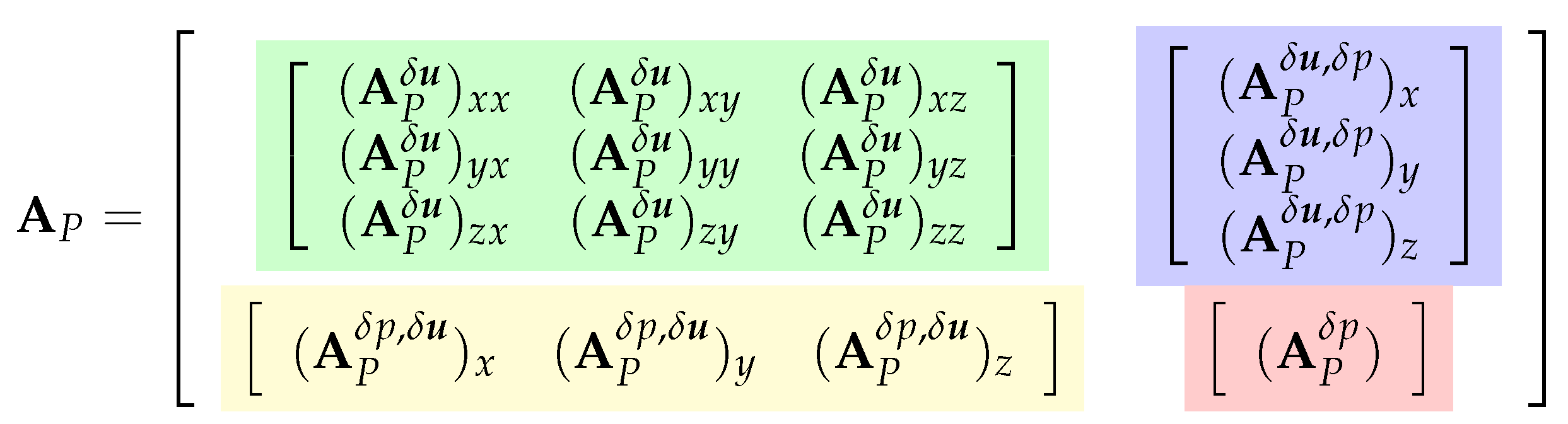
Figure 3.
Geometry of the spatial computational domain for the flat plate with a circular hole (, , , , ).
Figure 3.
Geometry of the spatial computational domain for the flat plate with a circular hole (, , , , ).
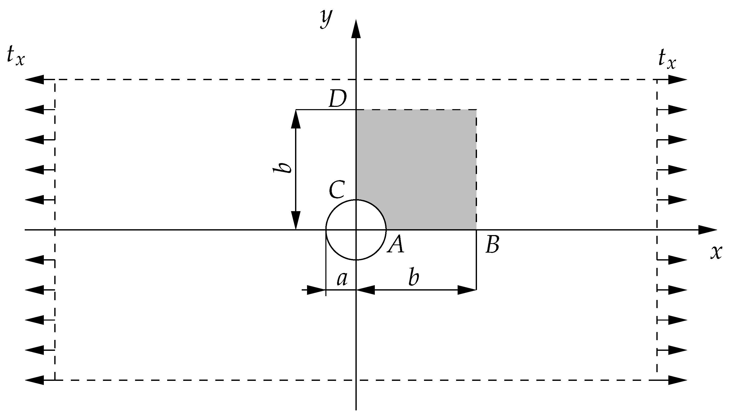
Figure 4.
Plate with a circular hole discretised using three cell types at comparable resolution: (a) quadrilateral cells, (b) triangular cells, and (c) polygonal cells.
Figure 4.
Plate with a circular hole discretised using three cell types at comparable resolution: (a) quadrilateral cells, (b) triangular cells, and (c) polygonal cells.
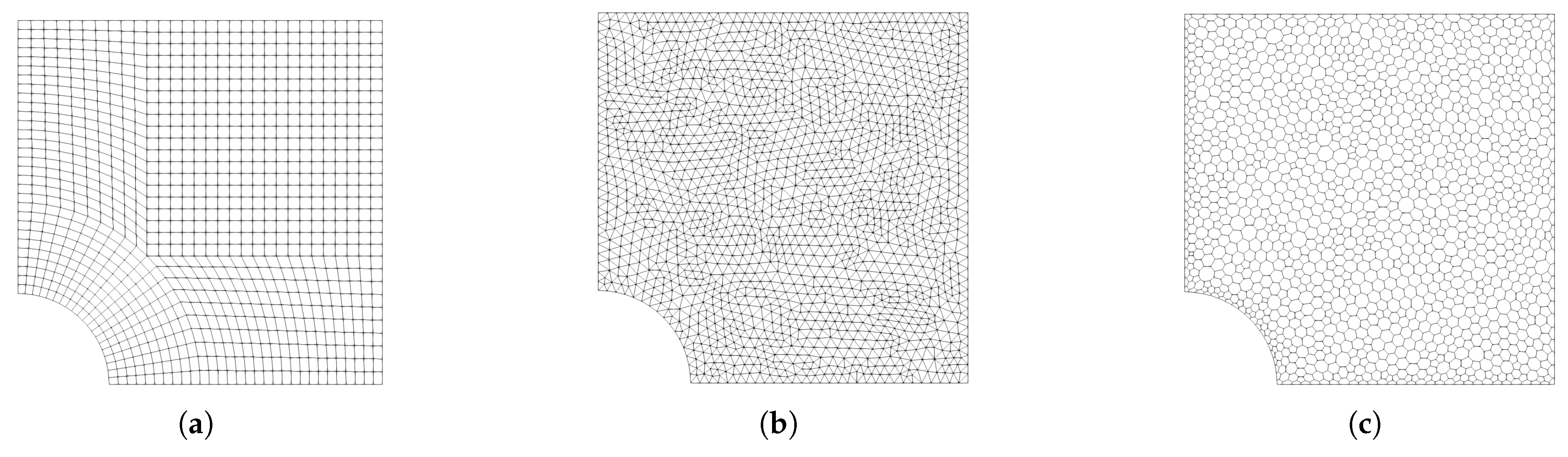
Figure 5.
Plate with a circular hole. Comparison of (a) the x-component of the displacement and (b) the -component of the Cauchy stress along the boundary of the spatial domain (see Figure 3).
Figure 5.
Plate with a circular hole. Comparison of (a) the x-component of the displacement and (b) the -component of the Cauchy stress along the boundary of the spatial domain (see Figure 3).
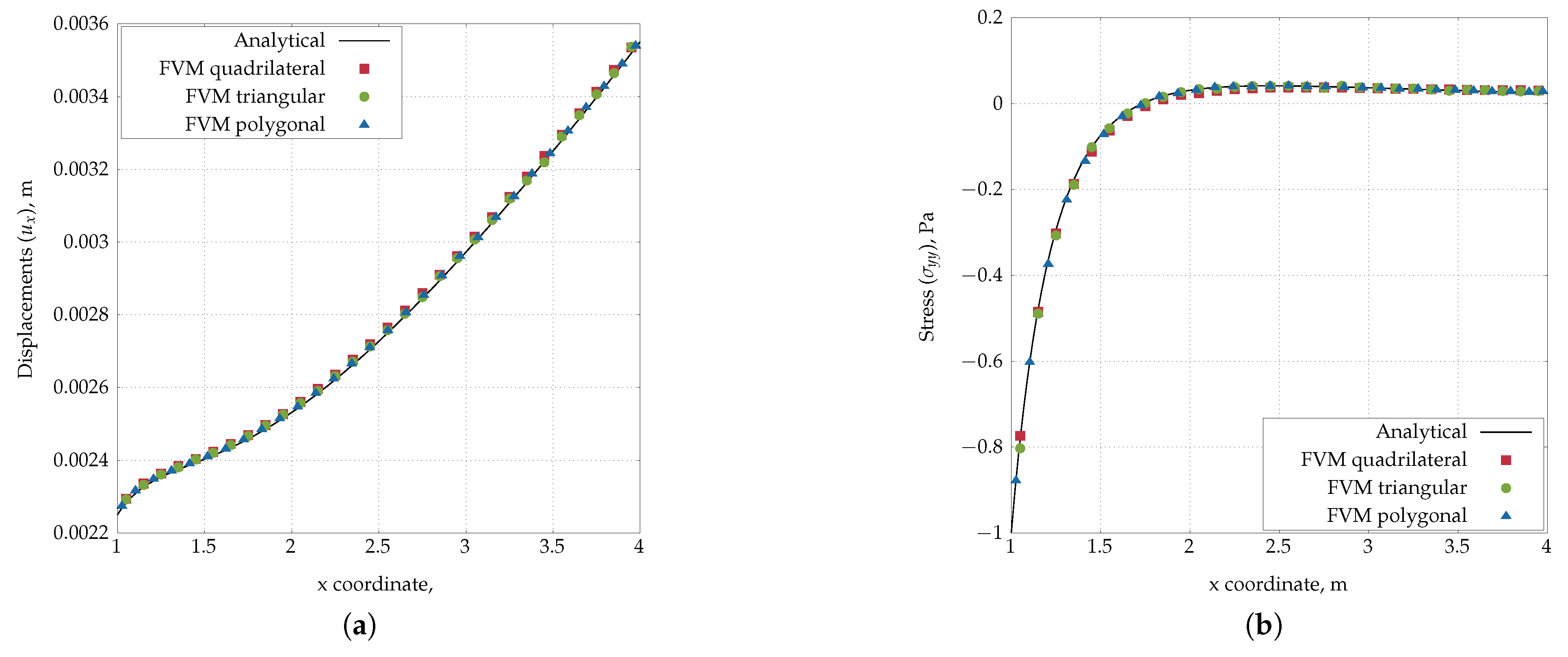
Figure 6.
Plate with a circular hole. Comparison of (a) the y-component of the displacement and (b) the -component of the Cauchy stress along the boundary of the spatial domain (see Figure 3).
Figure 6.
Plate with a circular hole. Comparison of (a) the y-component of the displacement and (b) the -component of the Cauchy stress along the boundary of the spatial domain (see Figure 3).
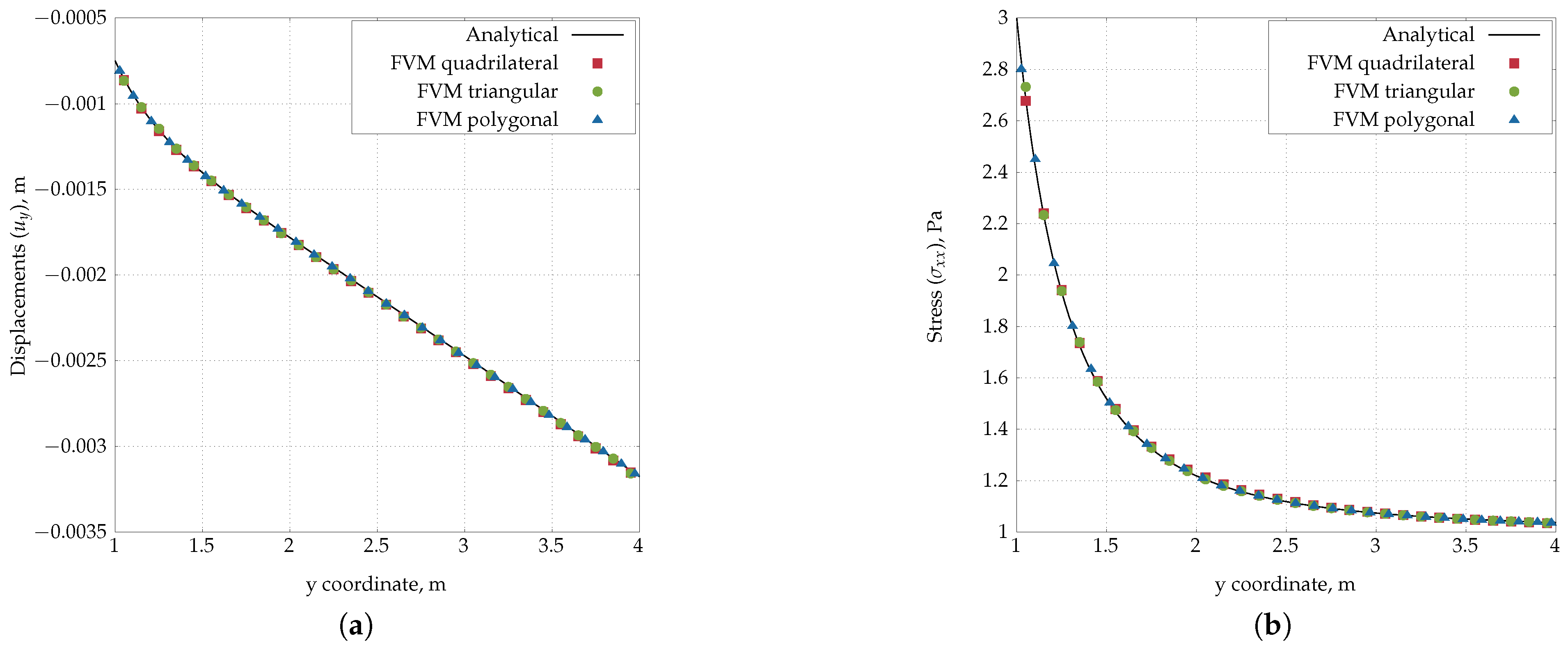
Figure 7.
Plate with a circular hole. Errors of (a) the displacement magnitude and (b) the -component of the Cauchy stress, calculated with respect to the analytical solution and evaluated by the , , and norms.
Figure 7.
Plate with a circular hole. Errors of (a) the displacement magnitude and (b) the -component of the Cauchy stress, calculated with respect to the analytical solution and evaluated by the , , and norms.
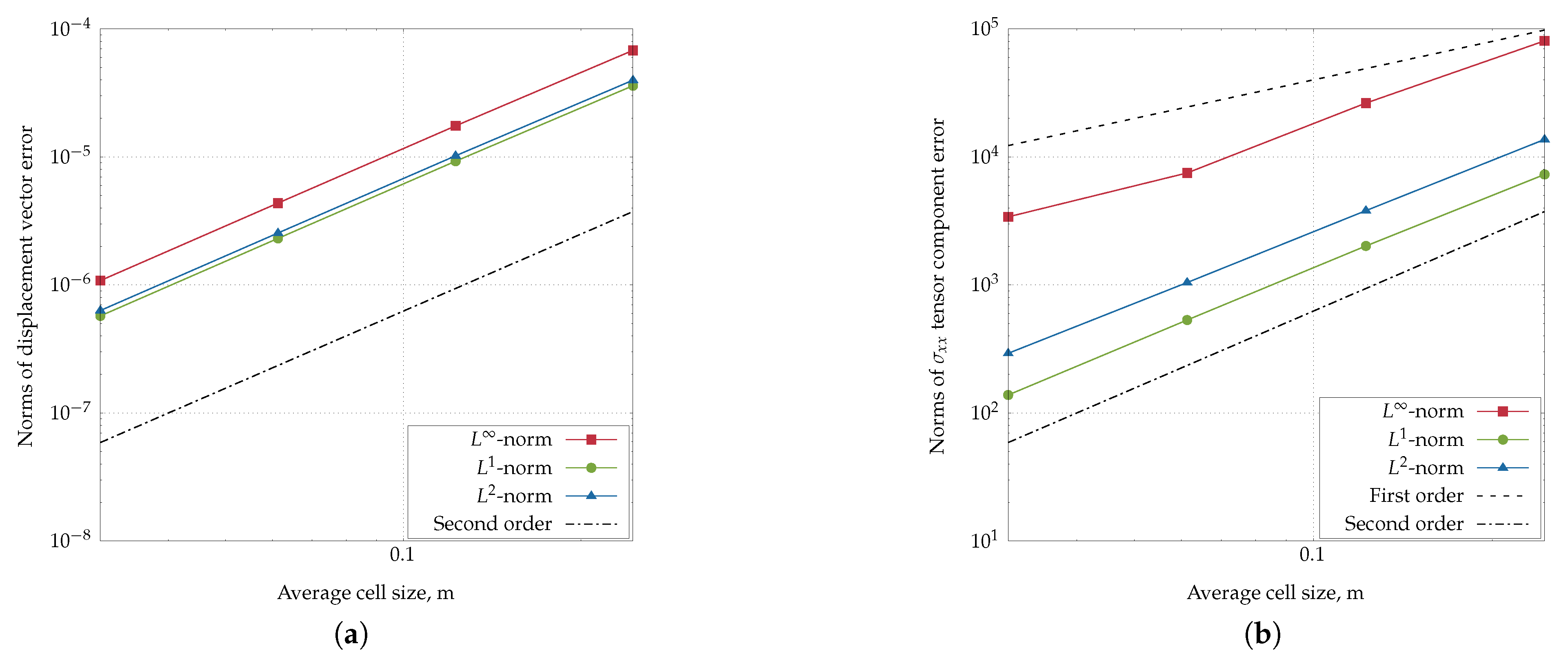
Figure 8.
Uniaxial extension of a block. Spatial domain in reference configuration and boundary conditions.
Figure 8.
Uniaxial extension of a block. Spatial domain in reference configuration and boundary conditions.
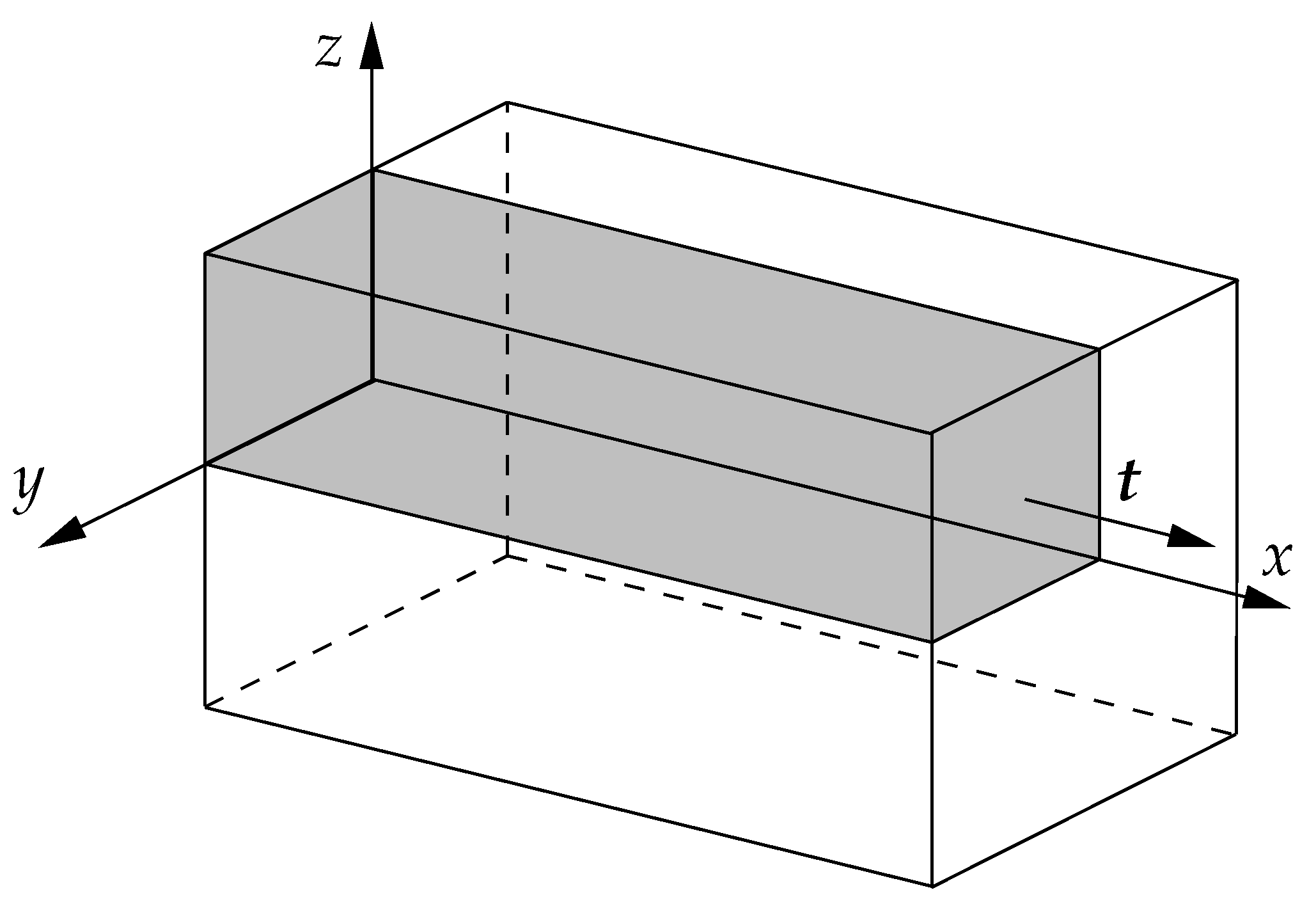
Figure 9.
Uniaxial extension of a block: reference configuration (black outline) and displacement field on the deformed configuration for .
Figure 9.
Uniaxial extension of a block: reference configuration (black outline) and displacement field on the deformed configuration for .
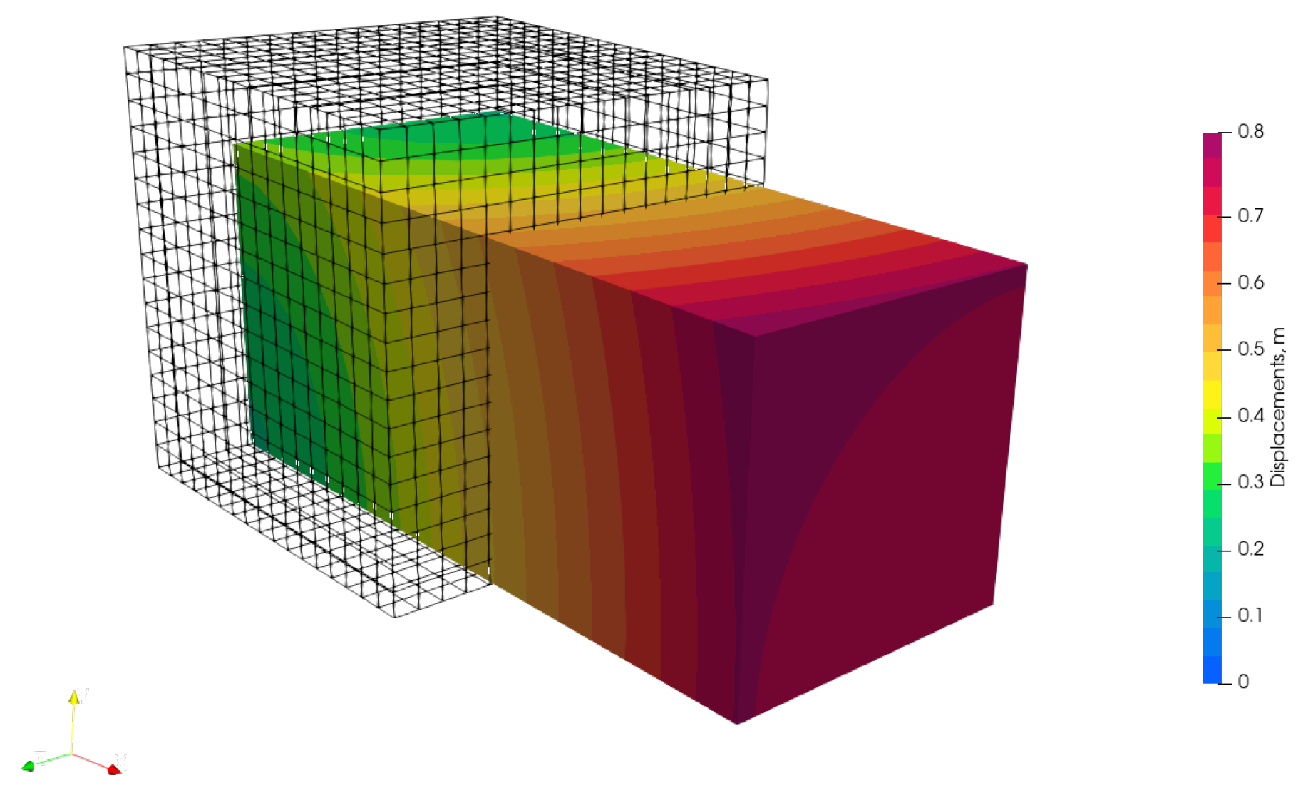
Figure 10.
Uniaxial extension of a block: analytical vs numerical results for the incompressible Neo-Hookean material. Plots of , , and pressure p as a functions of .
Figure 10.
Uniaxial extension of a block: analytical vs numerical results for the incompressible Neo-Hookean material. Plots of , , and pressure p as a functions of .
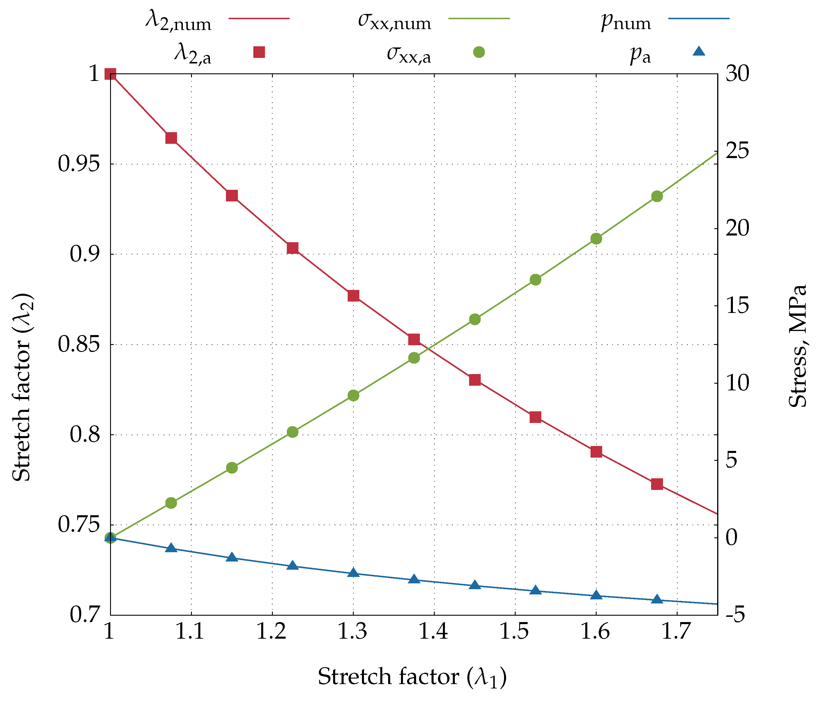
Figure 11.
Uniaxial extension of a block: analytical vs numerical results for the incompressible Guccione material. Plots of , , and pressure p as a functions of .
Figure 11.
Uniaxial extension of a block: analytical vs numerical results for the incompressible Guccione material. Plots of , , and pressure p as a functions of .
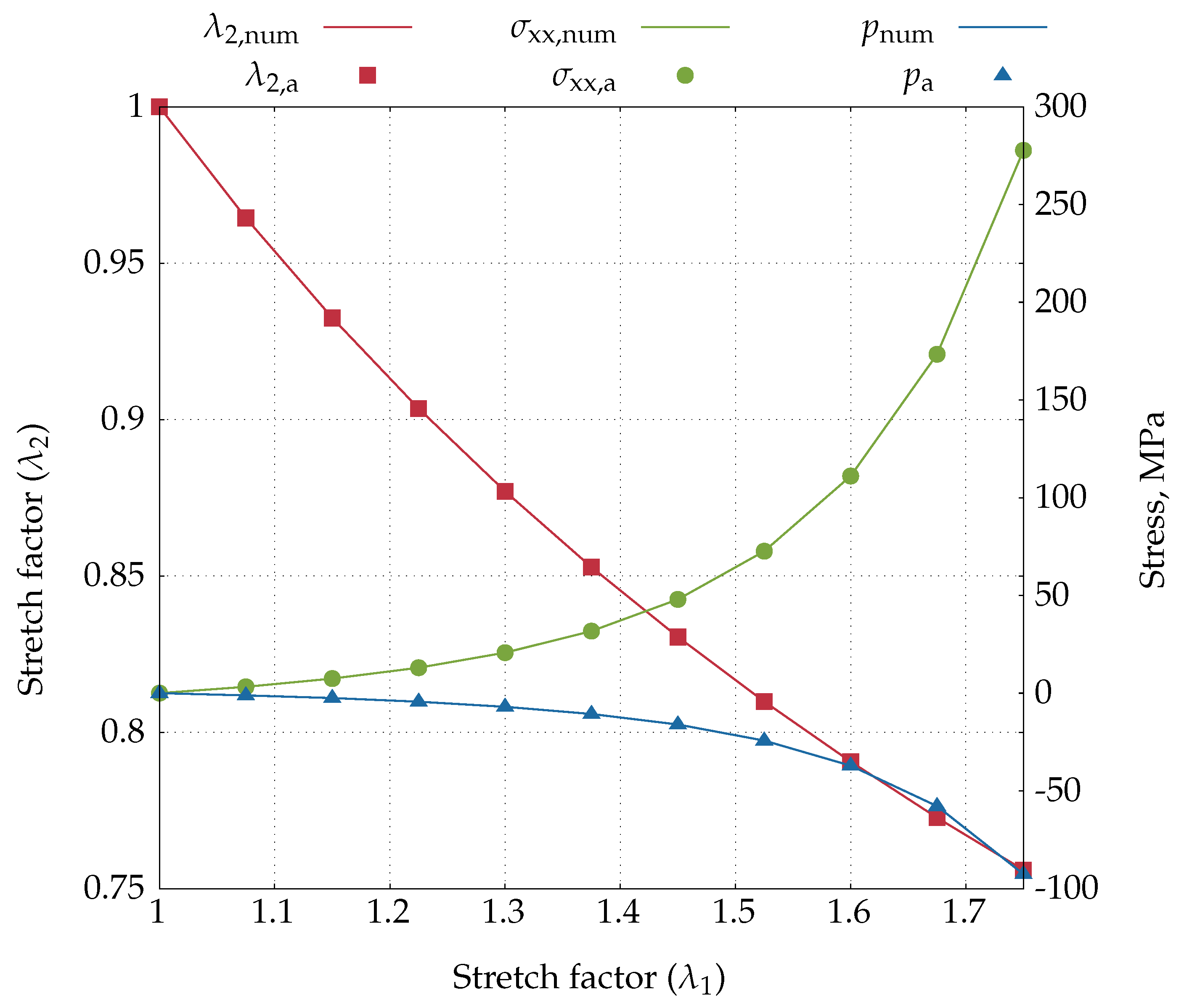
Figure 12.
Simple shear test of a unit cube: reference configuration and boundary conditions.
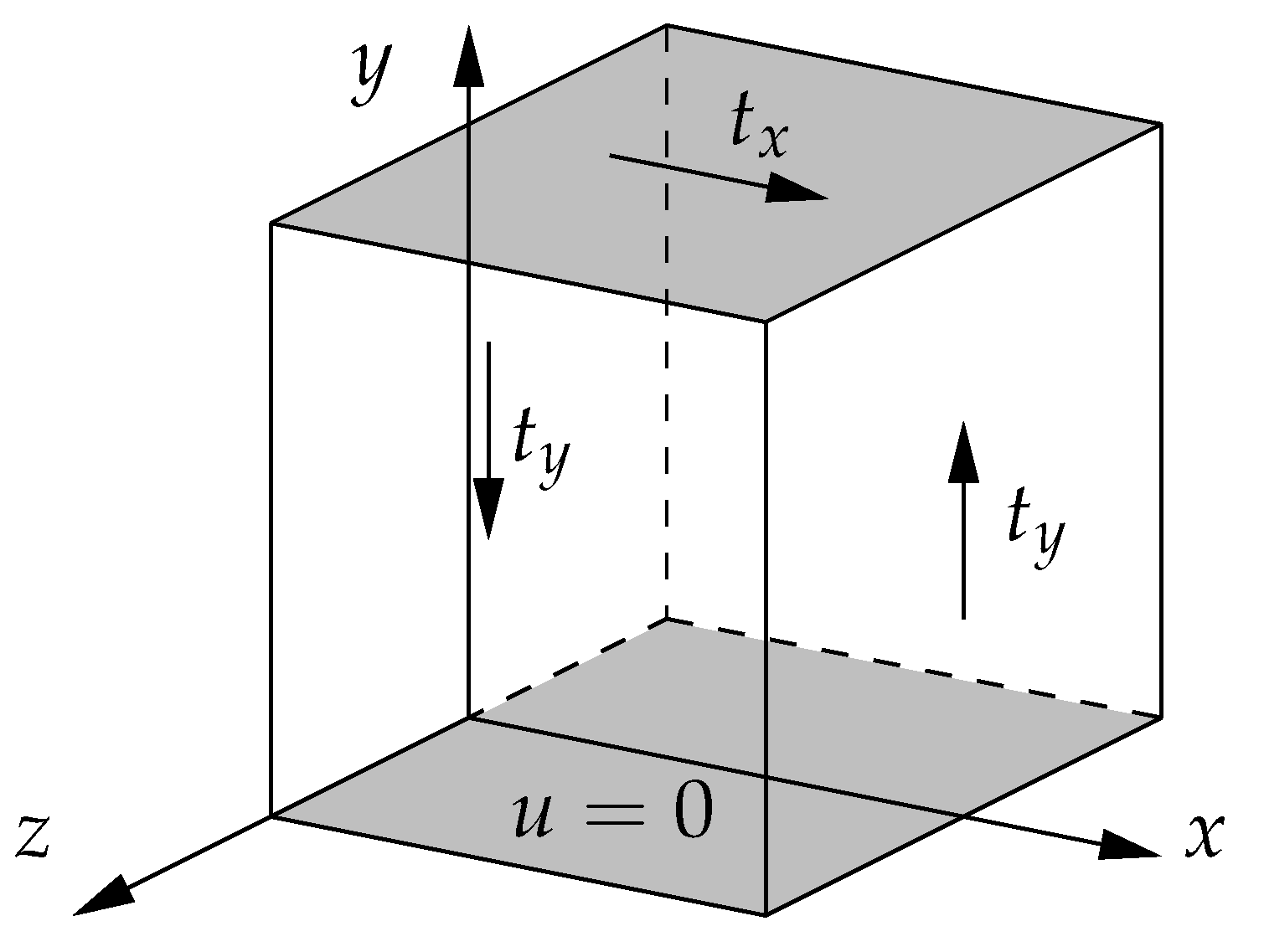
Figure 13.
Simple shear test: Current and reference configuration of the cube for shear strain obtained with the Neo-Hookean material model.
Figure 13.
Simple shear test: Current and reference configuration of the cube for shear strain obtained with the Neo-Hookean material model.
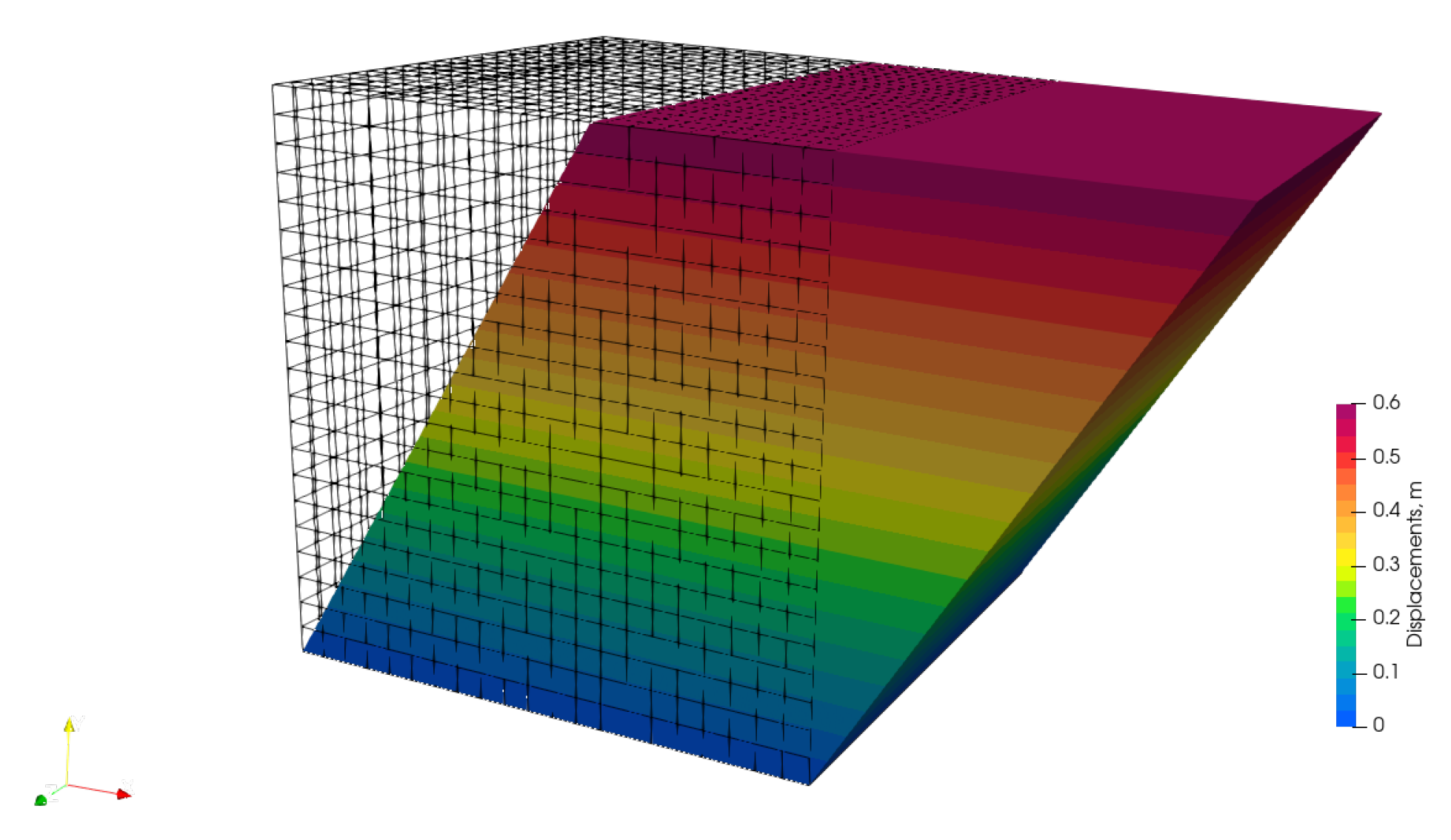
Figure 14.
Simple shear test: comparison of numerically computed top-surface displacement with the exact solution as a function of shear strain , for Neo-Hookean and Guccione material laws.
Figure 14.
Simple shear test: comparison of numerically computed top-surface displacement with the exact solution as a function of shear strain , for Neo-Hookean and Guccione material laws.
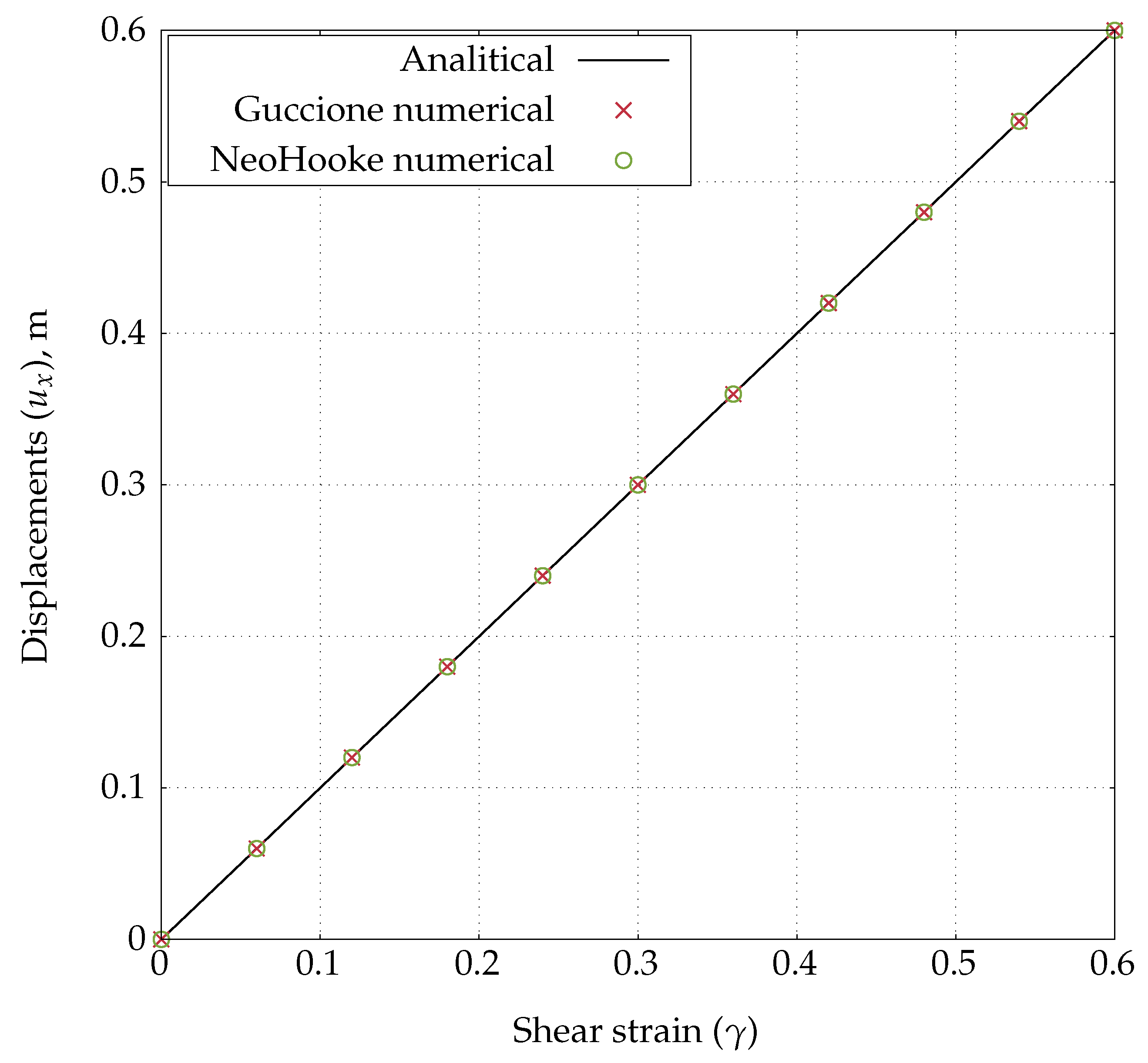
Figure 15.
Inflation of a pressurized cylinder: -section in reference configuration.
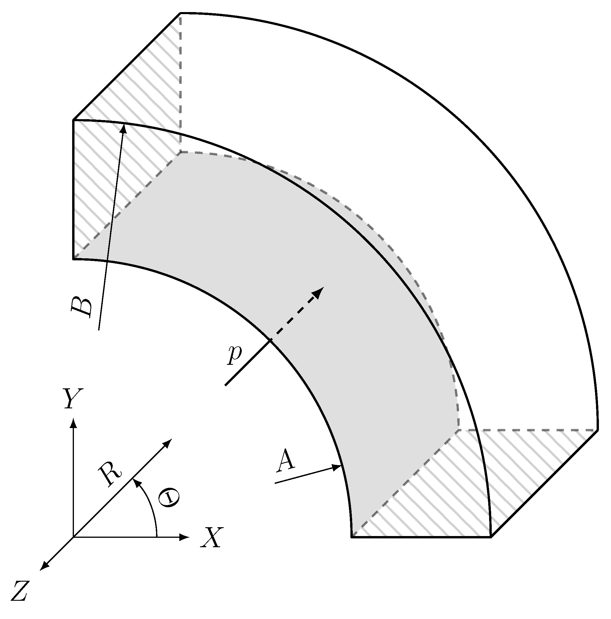
Figure 16.
Inflation of a pressurized cylinder: coarsest hexahedral mesh with 65 cells (a) and polyhedral mesh with 1,338 cells (b) used in the test case.
Figure 16.
Inflation of a pressurized cylinder: coarsest hexahedral mesh with 65 cells (a) and polyhedral mesh with 1,338 cells (b) used in the test case.
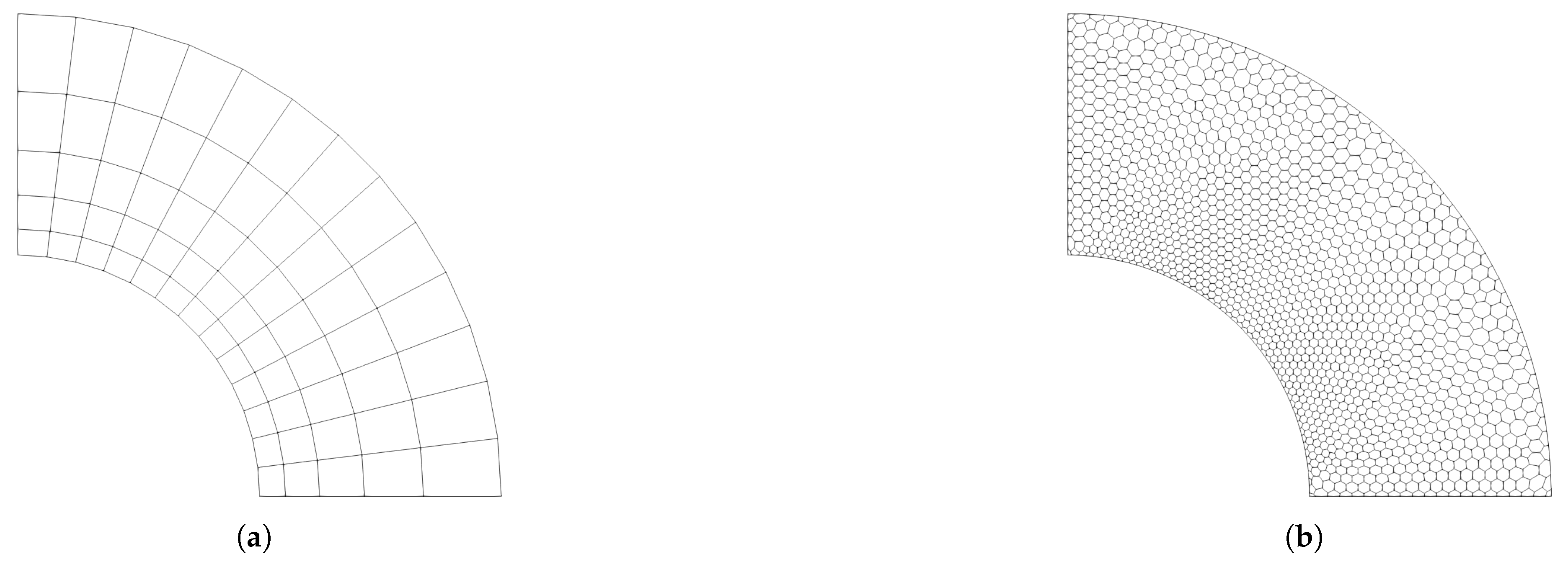
Figure 17.
Inflation of a pressurized cylinder: predicted results for three hexahedral meshes and one polyhedral mesh compared to the analytical solution.
Figure 17.
Inflation of a pressurized cylinder: predicted results for three hexahedral meshes and one polyhedral mesh compared to the analytical solution.
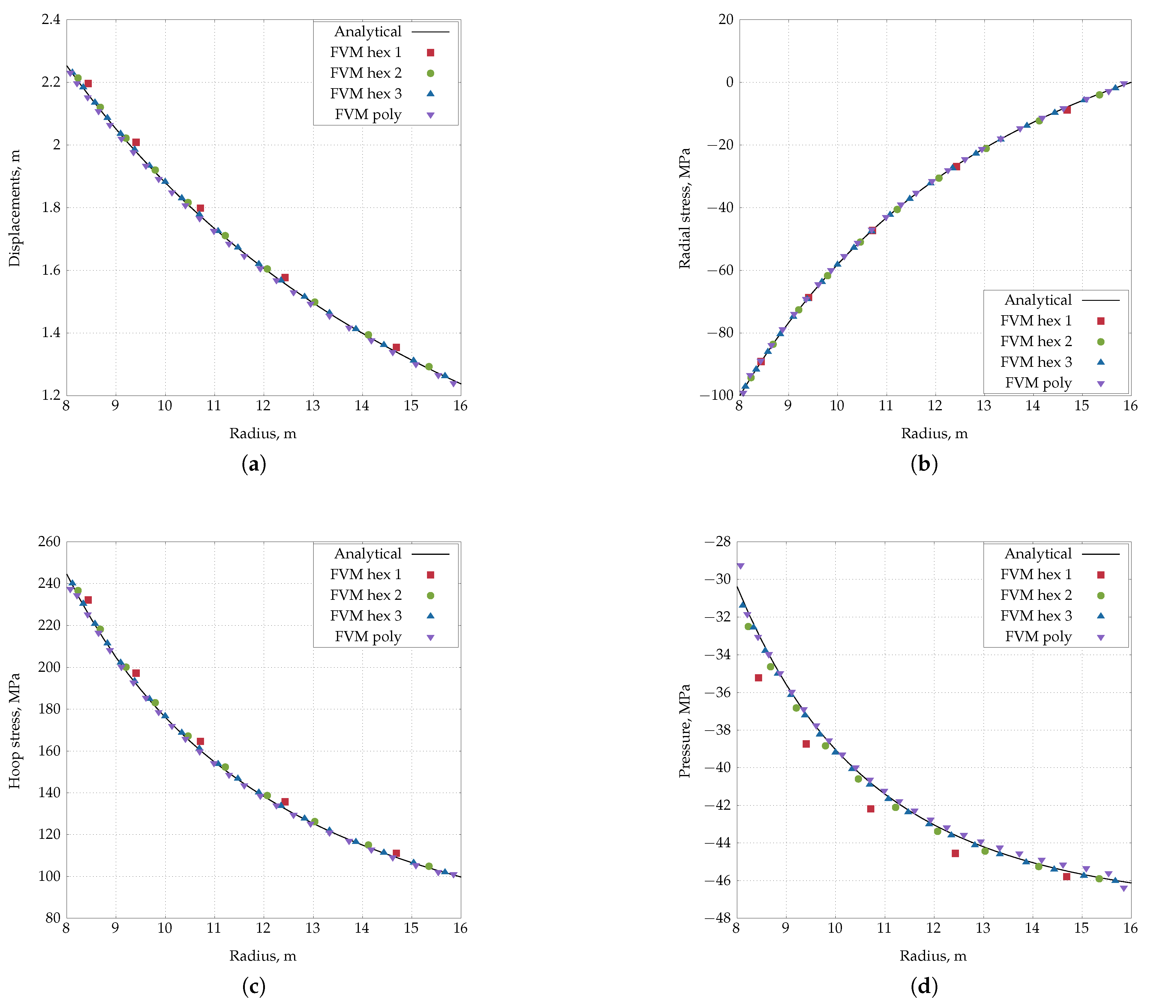
Figure 18.
Inflation of a pressurised cylinder: temporal accuracy study for Euler, backward Euler, composite, and Crank–Nicolson schemes using (a) the non-linear solver and (b) the linear solver.
Figure 18.
Inflation of a pressurised cylinder: temporal accuracy study for Euler, backward Euler, composite, and Crank–Nicolson schemes using (a) the non-linear solver and (b) the linear solver.
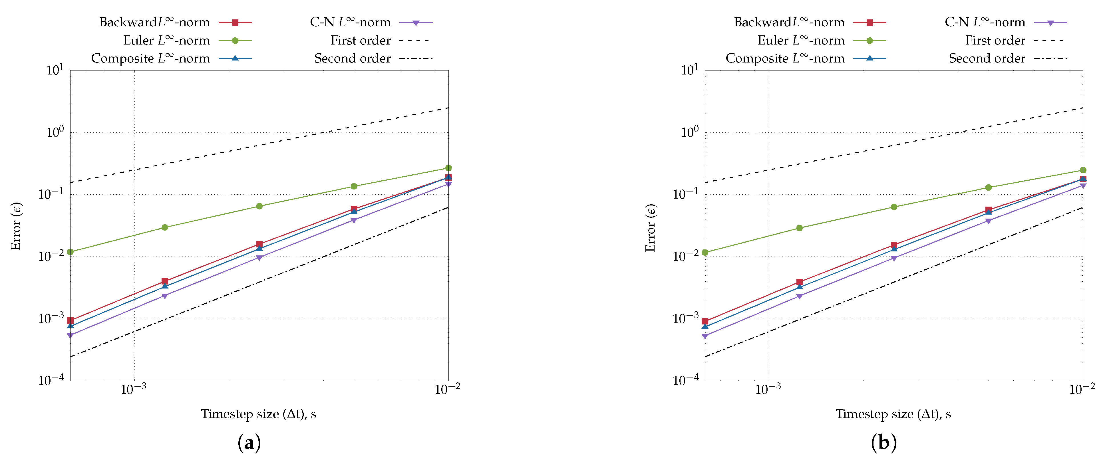
Figure 19.
Inflation of a pressurised cylinder: temporal evolution of the kinetic, elastic, and total energy of the system for the long-term response obtained using the backward temporal discretisation scheme.
Figure 19.
Inflation of a pressurised cylinder: temporal evolution of the kinetic, elastic, and total energy of the system for the long-term response obtained using the backward temporal discretisation scheme.
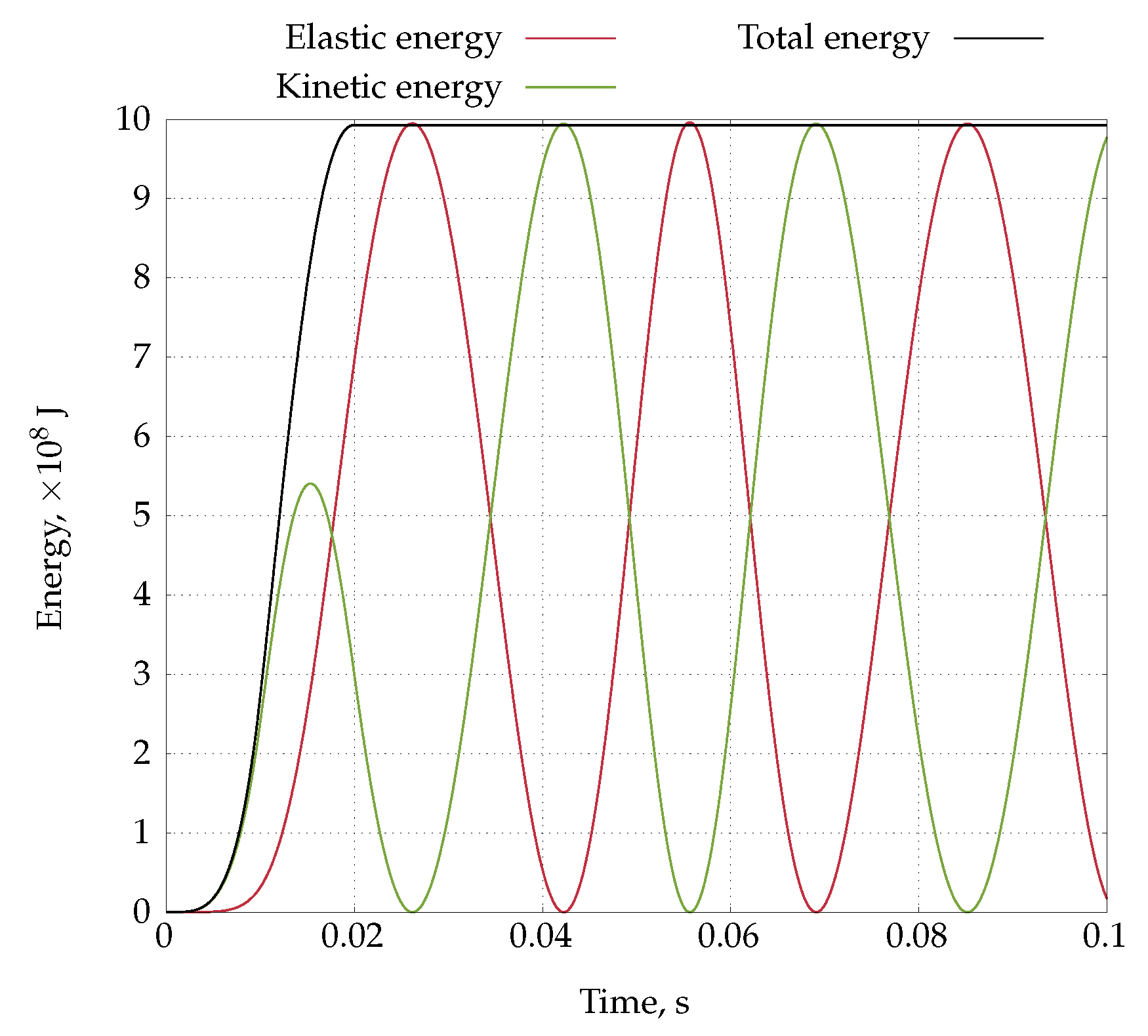
Figure 28.
Inflation of a rat carotid artery: reference configuration with mesh (one-quarter cylindrical domain) and deformed configuration at the final loading step, coloured by the displacement field.
Figure 28.
Inflation of a rat carotid artery: reference configuration with mesh (one-quarter cylindrical domain) and deformed configuration at the final loading step, coloured by the displacement field.
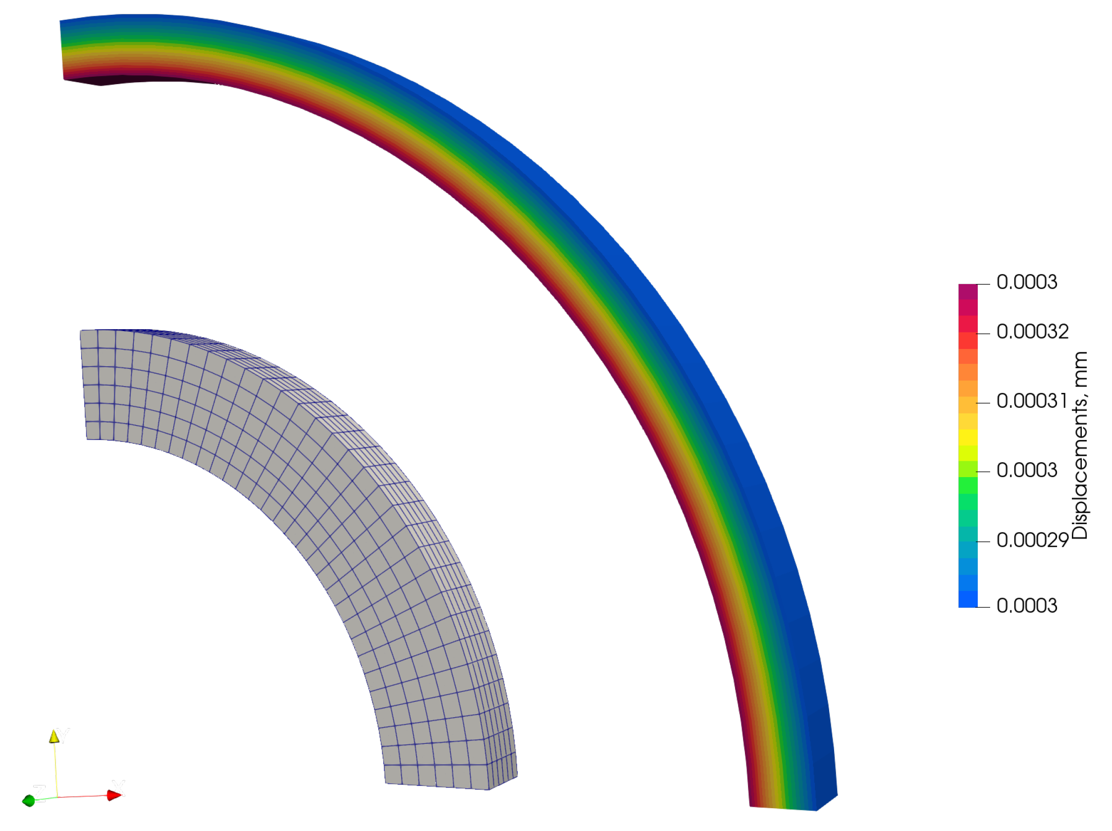
Figure 29.
Inflation of a rat carotid artery: the variation of the inner radius with respect to internal pressure (a), and the corresponding variation of outer radius (b).
Figure 29.
Inflation of a rat carotid artery: the variation of the inner radius with respect to internal pressure (a), and the corresponding variation of outer radius (b).
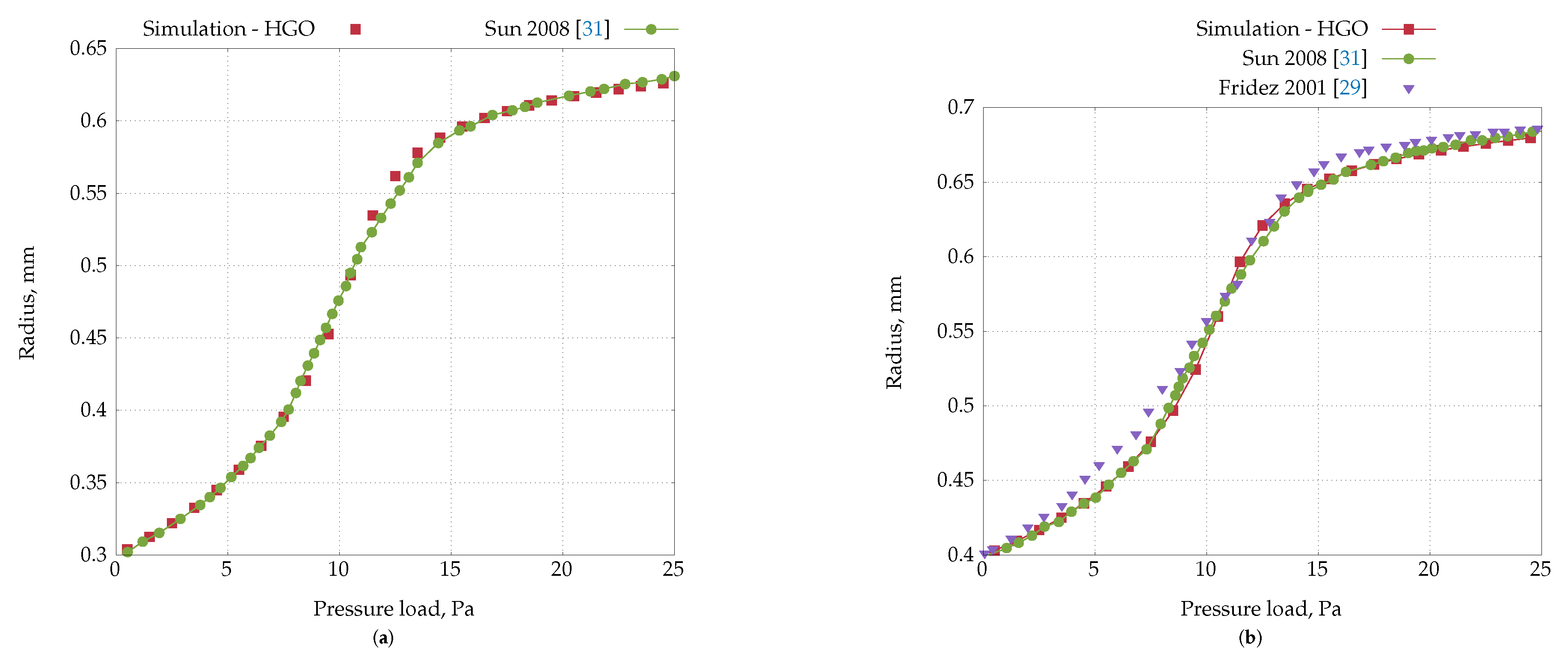
Figure 30.
Inflation of an idealized ventricle in the reference configuration. The entire domain is shown on the left; the computational domain (one quarter of the whole domain) is shown on the right.
Figure 30.
Inflation of an idealized ventricle in the reference configuration. The entire domain is shown on the left; the computational domain (one quarter of the whole domain) is shown on the right.
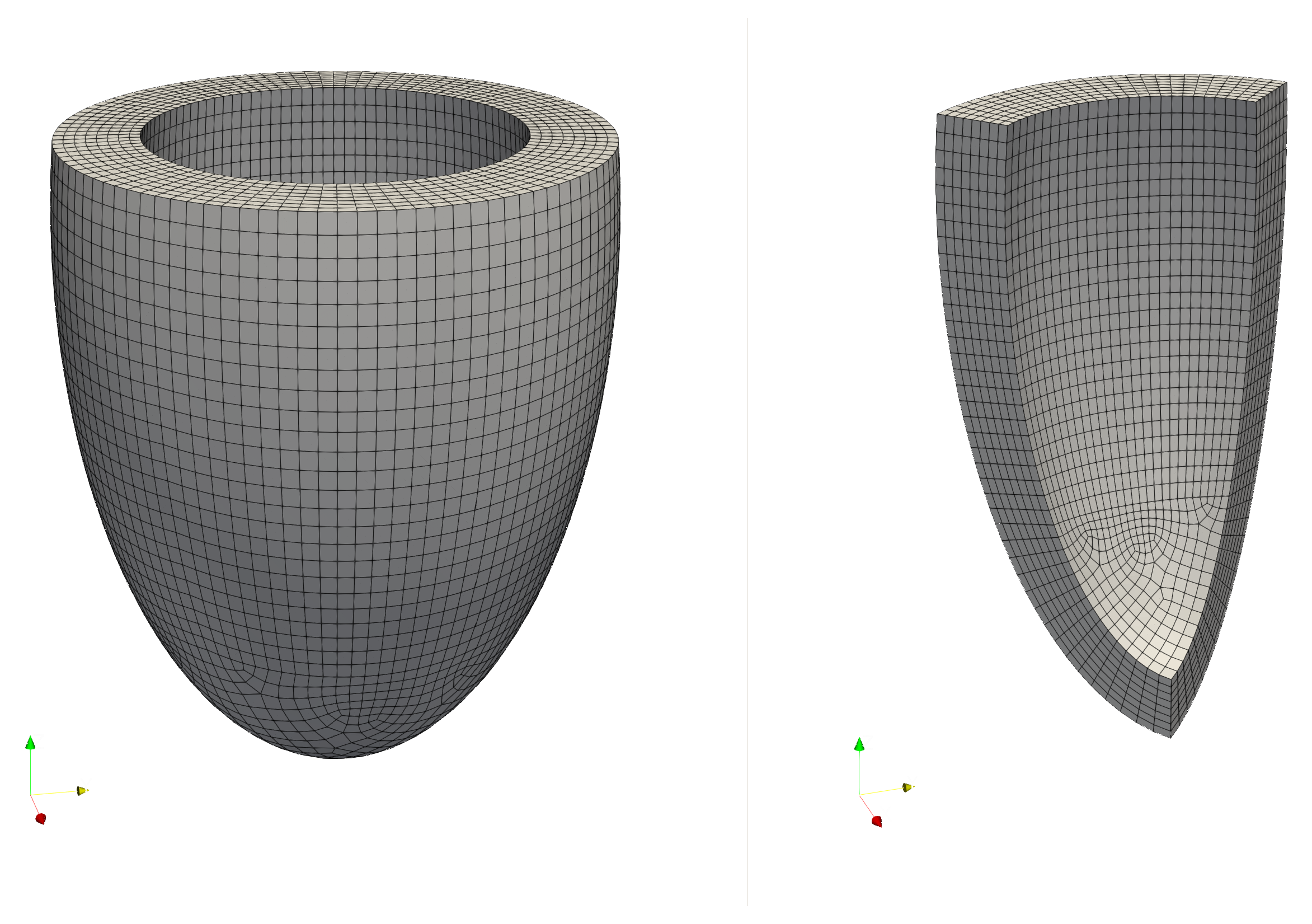
Figure 31.
Ventricle inflation: comparison of the apex displacement at the endocardial and epicardial surfaces during ventricular inflation, obtained using FV and FE simulations.
Figure 31.
Ventricle inflation: comparison of the apex displacement at the endocardial and epicardial surfaces during ventricular inflation, obtained using FV and FE simulations.
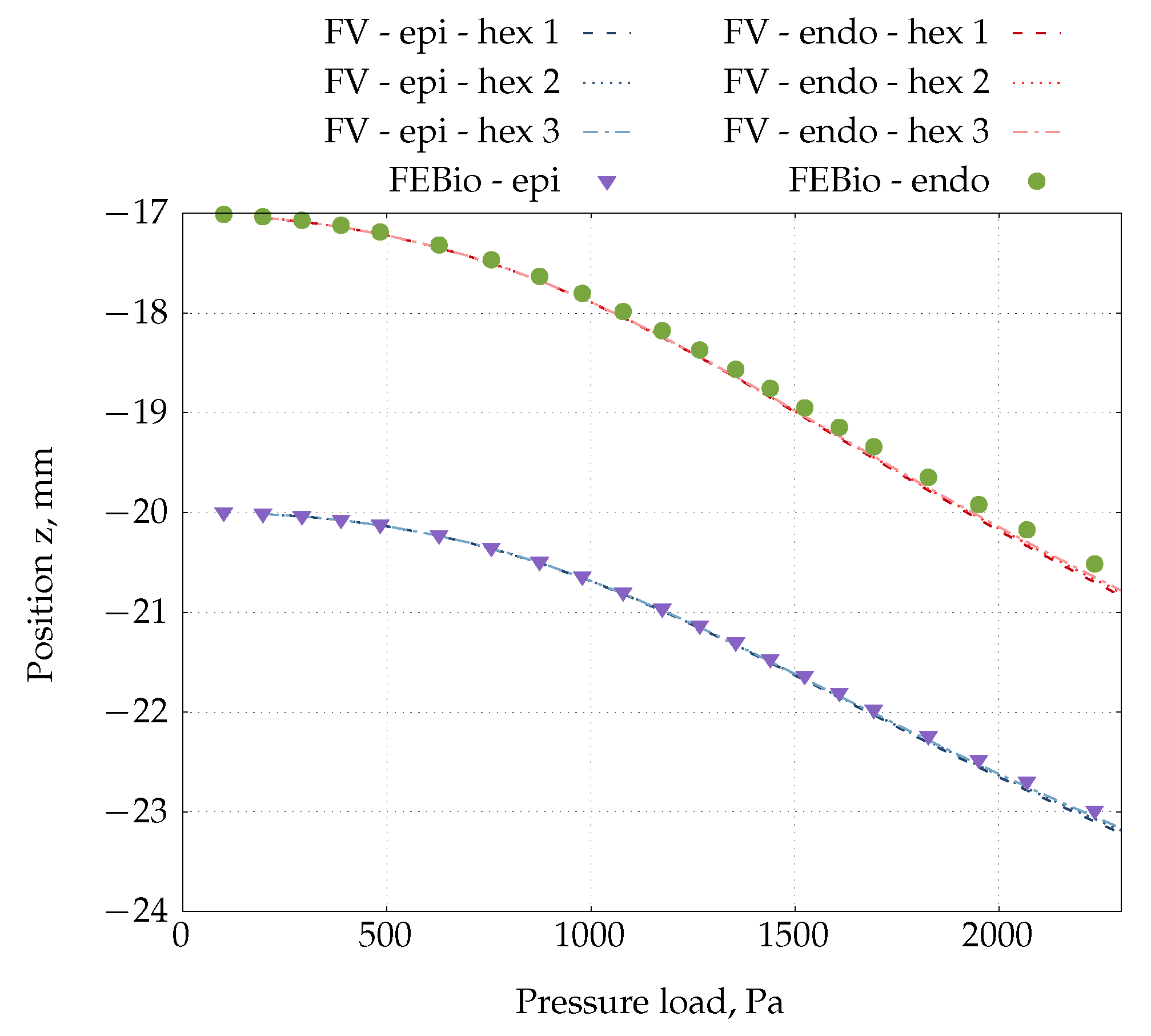
Figure 32.
Inflation of an idealised ventricle: deformed configuration of the ventricle wall midline obtained using FV and FE solvers for loading pressure .
Figure 32.
Inflation of an idealised ventricle: deformed configuration of the ventricle wall midline obtained using FV and FE solvers for loading pressure .
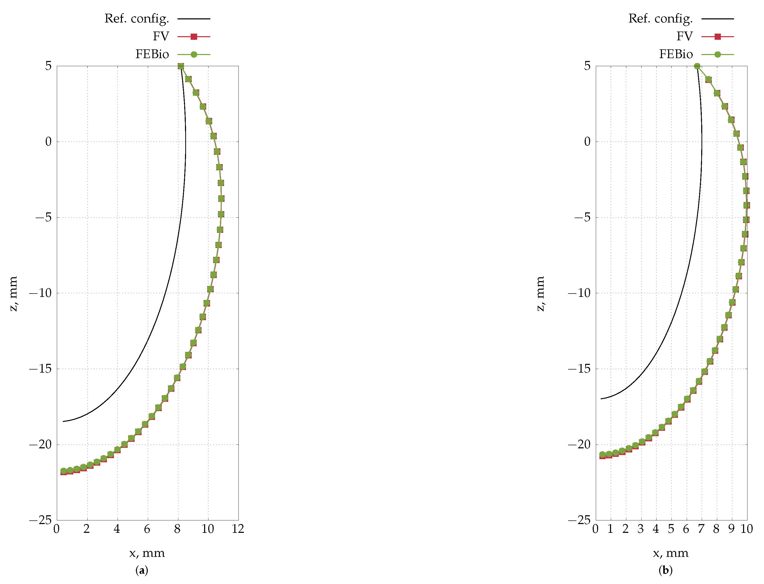
Figure 33.
Inflation of an idealised ventricle: comparison of the apex displacement at the endocardial and epicardial surfaces during ventricular inflation, obtained using FV and FE simulations for Neo-Hookean material.
Figure 33.
Inflation of an idealised ventricle: comparison of the apex displacement at the endocardial and epicardial surfaces during ventricular inflation, obtained using FV and FE simulations for Neo-Hookean material.
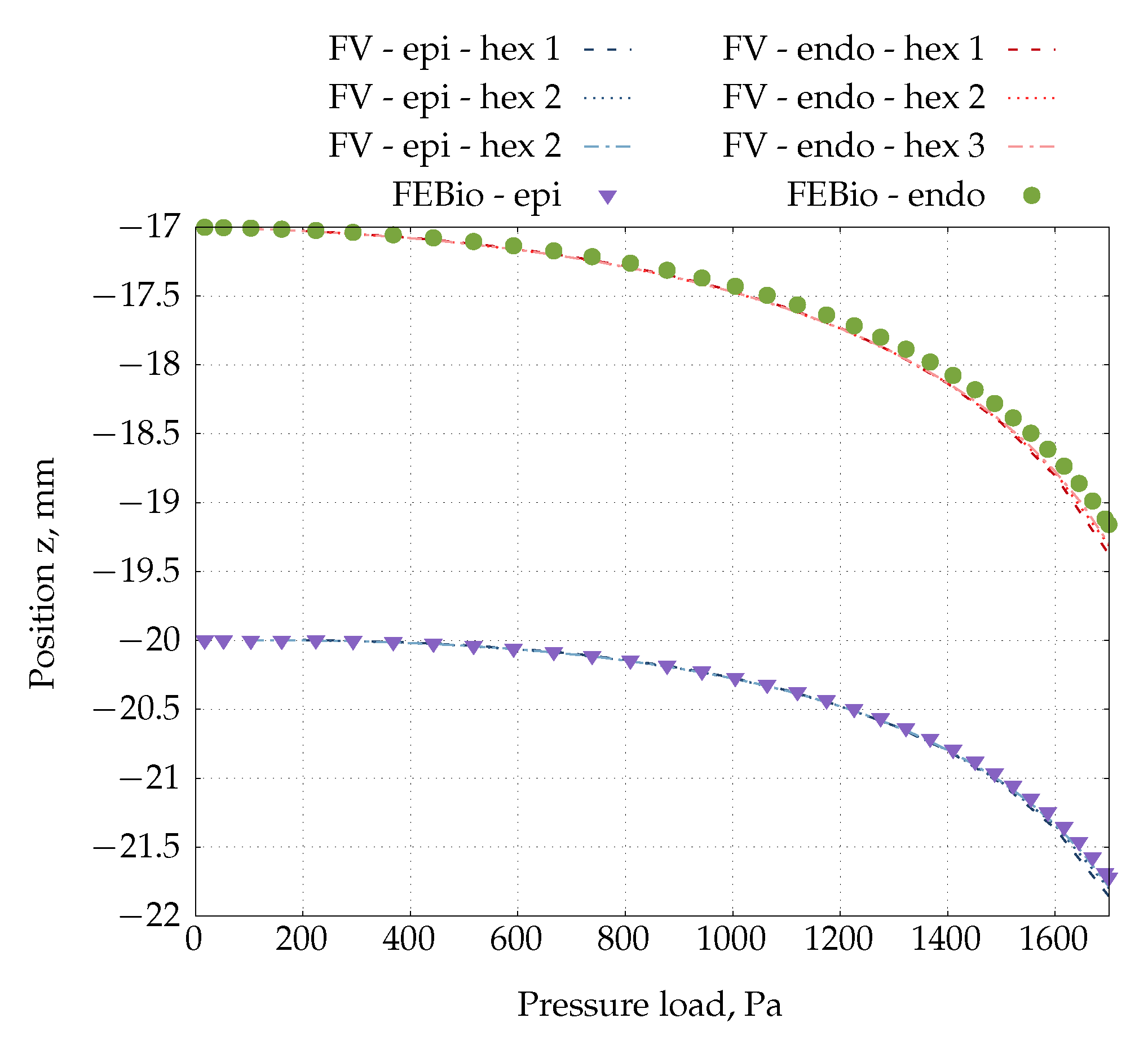
Figure 34.
Inflation of an idealised ventricle: deformed configuration of the ventricle wall midline obtained using FV and FE solvers for loading pressure with Neo-Hookean material.
Figure 34.
Inflation of an idealised ventricle: deformed configuration of the ventricle wall midline obtained using FV and FE solvers for loading pressure with Neo-Hookean material.
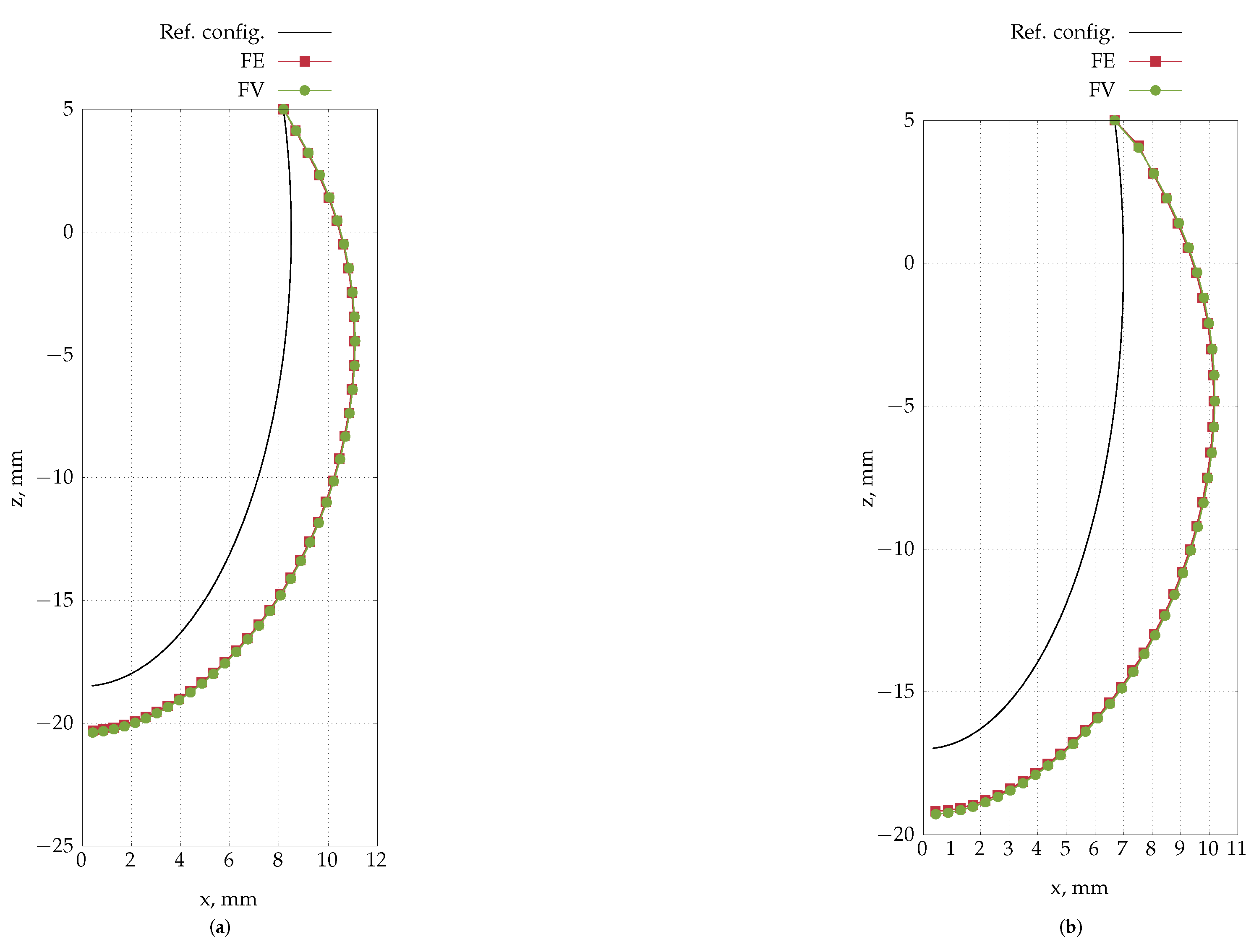
Disclaimer/Publisher’s Note: The statements, opinions and data contained in all publications are solely those of the individual author(s) and contributor(s) and not of MDPI and/or the editor(s). MDPI and/or the editor(s) disclaim responsibility for any injury to people or property resulting from any ideas, methods, instructions or products referred to in the content. |
© 2025 by the authors. Licensee MDPI, Basel, Switzerland. This article is an open access article distributed under the terms and conditions of the Creative Commons Attribution (CC BY) license (http://creativecommons.org/licenses/by/4.0/).
Copyright: This open access article is published under a Creative Commons CC BY 4.0 license, which permit the free download, distribution, and reuse, provided that the author and preprint are cited in any reuse.


