colorlinks=true, linkcolor=black, citecolor=black, urlcolor=black
1. Introduction
Positioning & Scope. This section motivates the problem and clarifies the paper’s scope for the present framework: we aim at a symmetry-based, conditionally luminal tensor sector at quadratic order, not at a full replacement of ΛCDM or a comprehensive cosmological fit. Our contribution is foundational: it identifies astructuralroute to under explicit assumptions (A1–A6), and it frames a clear, falsifiable NLO prediction accessible to multi-band GW data.
The dawn of multimessenger astronomy, heralded by the joint observation of gravitational waves (GW170817) and a gamma-ray burst (GRB170817A), has transformed fundamental physics [
28,
29]. The near-simultaneous arrival of these signals established that gravitational waves propagate at the speed of light to an astonishing precision,
. This single measurement acts as a stringent filter for a vast landscape of modified gravity theories. While some models can be salvaged by fine-tuning parameters, such an approach is often considered theoretically unnatural. This predicament sharpens a fundamental question:
Can we construct a gravitational theory where luminal tensor speed is a direct consequence of an underlying symmetry principle, rather than an accident of parameter choice?
This paper provides an affirmative answer within a first-order, Palatini-type geometry endowed with torsion. We propose that the observable sector of gravity is governed by two key symmetry principles:
A Scalar PT Projection: We postulate that all observable scalar densities are projected into a PT-even (parity-time symmetric) subspace. This acts as a selection rule, ensuring that the action is real and the Hamiltonian is Hermitian, while systematically eliminating potential parity-odd effects like gravitational birefringence at leading order.
Projective Invariance: We implement projective symmetry via a non-dynamical Stueckelberg compensator field , which can be intuitively understood as a geometric phase. This ensures that observables are only sensitive to the projectively invariant trace of torsion, , structurally avoiding extra propagating degrees of freedom that often plague torsionful theories.
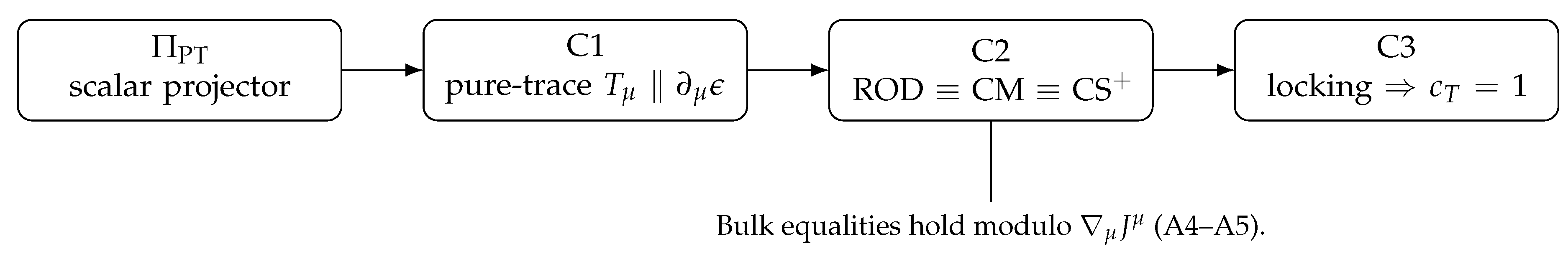
Within this symmetric and self-consistent posture, formalized by six assumptions (A1–A6) in Section 2, we derive a cascade of powerful, conditional results at the quadratic action level. As illustrated in
Figure 1, these principles first act as a structural constraint that aligns the torsion into a unique pure-trace form (Result C1). This simplification then reveals a remarkable bulk equivalence between three distinct theoretical routes (Result C2).
The culmination of this structure is a novel coefficient locking mechanism (Result C3). Demanding the absence of unphysical mixing between tensor modes and non-propagating fields fixes a unique relationship between the theory’s building blocks. This locking forces the kinetic (K) and gradient (G) terms in the tensor action to be identical up to a boundary term. This identity, , structurally ensures an exactly luminal tensor speed () by construction. This result is algebraic, requires no parameter tuning, and emerges directly from the imposed symmetries.
The framework’s utility lies not only in its structural elegance but also in its predictive power. It yields a distinctive, testable signature at the next-to-leading order (NLO) that is absent in standard General Relativity: a frequency-dependent deviation in the speed of gravity given by
where
k is the wavenumber and
is the effective energy scale of new physics. A detection of this specific
scaling in future multi-band GW data (from Pulsar Timing Arrays, LISA, and next-generation detectors) would provide a powerful probe of spacetime’s fundamental geometry, while its absence would falsify the framework. This paper lays out the theoretical foundations, proves the core properties, and details the clear, falsifiable predictions of this symmetry-based approach.
2. The Theoretical Posture: Symmetries, Assumptions, and Projectors
Positioning & Scope. We specify the working posture and its admissible variational domains. The two-derivative truncation and the spurion limit are deliberate, conservative choices ensuring a real, -even scalar sector while preserving projective invariance in observables. All claims in later sections are to be read strictlyunderassumptions A1–A6 and on admissible boundaries; outside this posture no general statements are implied.
This section fixes the theoretical foundation of our framework. We begin by stating the two guiding principles already previewed in
Section 1: (i) projective invariance in observables, implemented via a Stueckelberg compensator, and (ii) a scalar
projection that enforces reality at the level of observable densities. We then formalize the complete set of assumptions (A1–A6) defining our working posture, and finally define the scalar
projector and its key properties. All constructions are performed within a metric-compatible Palatini formalism on an oriented
-dimensional spacetime, with torsion
and curvature
.
2.1. Principle 1: Projective Symmetry and the Stueckelberg Spurion
Our first guiding principle is projective symmetry, a standard redundancy of Palatini geometry under which the affine connection shifts without changing the curvature tensor:
To ensure physical observables are invariant under (
3), we introduce a Stueckelberg compensator field
and assign it the compensating transformation
. This allows the theory to be organized in terms of the
projectively invariant torsion-trace combination
Within our two-derivative truncation we adopt a spurion limit: is treated as a non-dynamical background field at this order. Consequently, admissible observables may depend on only through the invariant combination . This conservative choice preserves projective invariance while enabling the algebraic simplifications central to our results.
2.2. Optional UV Motivation: A PTQ Interpretation (Not a Premise)
Positioning & Scope. This subsection isinterpretiveand optional. It provides one natural UV narrative for the compensator and for the scalar- projection, butnoneof the proofs in this paper depend on that narrative. All structural results (C1–C3) rely only on the spurion/projective-invariant chain under the posture A1–A6.
Why include an optional UV interpretation?
The posture adopted here—a non-dynamical Stueckelberg compensator entering only through
and a scalar-
projection acting on observable densities—is fully consistent as a conservative two-derivative effective framework. Nevertheless, it is conceptually useful to note that the same pattern can arise as a particularly economical low-energy remnant of a richer UV completion. One such UV viewpoint is a PT-symmetric quaternionic-spacetime (PTQ) interpretation, in which
is naturally read as a phase/clock-like geometric spurion and the scalar-
projection acts as a reality filter on the observable sector. We emphasize that this PTQ narrative is a
motivation and a
roadmap for deepening the theory, not an additional assumption.
1
Minimal mapping (interpretive only).
From a PTQ perspective, the two guiding principles may be viewed as IR footprints of a UV structure:
Projective invariance as an IR gauge redundancy. A projective shift of the Palatini connection may be interpreted as an emergent redundancy after integrating out heavy UV modes, leaving only the invariant combination in observables. In this reading, is the minimal Stueckelberg spurion that packages UV phase information into the IR without introducing additional propagating degrees of freedom at quadratic order.
Scalar- projection as a selection rule on observables. A PTQ-inspired completion naturally motivates imposing a reality condition at the level of scalar densities (rather than on all microscopic fields). Operationally, this is exactly what implements in our posture: it retains the -even scalar sector in observables while keeping the underlying geometric variables otherwise standard within metric-compatible Palatini gravity.
What depends on PTQ (and what does not).
To prevent over-reading, we explicitly separate structure from interpretation:
Independent of PTQ: The operator basis, Palatini algebraicity, the uniqueness map (C1), the three-route bulk equivalence (C2), and the coefficient-locking identity enforcing (C3) follow solely from A1–A6 together with the spurion/projective-invariant construction and standard variational identities.
PTQ as a UV guide (optional): PTQ provides a plausible UV interpretation for why a non-dynamical phase-like spurion and a scalar-level selection may be stable low-energy remnants, and it offers an intuitive reading of the EFT cutoff entering NLO dispersion as a scale at which additional UV degrees of freedom would become dynamical.
Practical takeaway.
In short, PTQ is the more ambitious version of the story—it suggests a concrete UV direction and a principled origin for —but the present paper deliberately treats it as non-essential. The main claims are symmetry-protected and auditable within the spurion/projective-invariant posture, regardless of which UV completion one ultimately adopts (PTQ or otherwise).
2.3. Principle 2: The Scalar Projector and Reality of Observables
Our second guiding principle is to project observable scalar densities onto a real, -even subspace. Operationally, this acts as a “reality filter” at the level of observables: the projected action is real by construction, and the quadratic operators governing physical perturbations are Hermitian within the posture specified below.
Why on scalar densities?
On an oriented Lorentzian manifold, the combined transformation preserves the orientation of the spacetime volume element (A2). Imposing the reality condition at the level of scalar densities is the minimal intervention compatible with the Palatini variational principle: it does not require imposing on every microscopic field component, yet it ensures that all scalar observables entering the action are -even in the projected sector.
Connection to Hermiticity (within the posture).
We impose the projection on observable densities rather than as a microscopic constraint on . Within our admissible variational domains and with the spurion held fixed, the projection commutes with the Palatini variation (A3), so the resulting quadratic forms in the physical sector are Hermitian:
“-even projected scalar densities ⇒ real action density ⇒ Hermitian quadratic operators (in the projected sector).”
This statement is to be read strictly under A1–A6.
2.4. The Working Posture (Assumptions A1–A6)
The conditional results of this paper are derived under the following explicit assumptions, collectively referred to as our posture.
Note on admissible domains.
The posture admits standard, simply connected spacetimes. Manifolds with torsion defects, nontrivial holonomy for
, or multi-valued spurions could induce non-vanishing boundary fluxes and may spoil the bulk equivalences derived later (cf.
Section 5).
2.5. Formal Properties of the Projector
We now formalize the scalar projector and its essential properties.
Convention note (spurion charges).
We treat as a non-dynamical spurion field. Discrete P and T assignments for are chosen so that the invariant combination is compatible with the projected -even observable sector. This ensures that selection rules act consistently on the spurion-built scalars used below.
Action of P, T, and .
The transformations of key geometric objects under
P and
T are summarized in
Table 1. We emphasize that
T is anti-unitary: it includes complex conjugation on scalar coefficients.
Definition and core properties.
The projector onto the
-even subspace of scalar densities is defined by
Under assumption A1 (a -invariant integration domain/measure), this projection is self-adjoint in the sense appropriate for scalar densities on the admissible domain, and it defines a consistent restriction to a -even observable sector.
(A3)).Lemma 1 (Projection-Variation Commutation Under A1 and A4, if the spurion ϵ is held fixed (non-variational), then for variations of one has for any scalar density .
Proof. Linearity gives . On the admissible domain (A4), boundary improvements do not contribute to the symplectic form, and with held fixed the map acts only on the dynamical variations of and on complex conjugation (anti-unitarity of T). Therefore , implying the claim. □
Theorem 1 ( Selection Rules). Under the posture A1–A5, for any scalar density : (i) if , then ; (ii) if , then .
Proof. Immediate from the definition (
5). □
2.6. Summary of Key Ingredients
For clarity, we consolidate the key spurion-built variables that constitute the observable scalar sector in this framework.
3. Building the Operator Basis: From Symmetries to Observables
Positioning & Scope. This section is technical by design and self-contained. It enumerates the complete quadratic, PT-even, projectively invariant basis before equations of motion (pre-lock), then shows its collapse after solving for the torsion (post-lock). The goal is transparency: all later identities are traceable to this basis and to integration-by-parts on admissible domains.
Having established our guiding principles and working posture, we now construct the complete basis of observable operators at the lowest non-trivial order (quadratic in fields, with at most one derivative per field). This systematic process is a crucial preparatory step. We first identify all operators allowed by the symmetries
before applying the equations of motion, defining the "pre-lock" basis. We then show how this basis simplifies once the dynamics are solved in
Section 4, yielding the "post-lock" sector. This ensures our theory is built from a complete and self-consistent set of building blocks.
Throughout this section, the posture A1–A6 defined in Section 2 is in force. All scalar densities are implicitly understood to be projected via , rendering them real and -even.
3.1. Symmetry-Allowed Building Blocks
The combined requirements of projective invariance and PT symmetry act as a powerful filter. As established in Section 2, all observables must be constructed from the projectively invariant trace of torsion, , and the Stueckelberg gradient itself.
At quadratic order with at most one derivative per field, Theorem 1 allows only three types of -even scalar monomials to survive the projection:
- (i)
The quadratic torsion invariant, built from .
- (ii)
The quadratic spurion-gradient invariant, .
- (iii)
The mixing term, .
Crucially, before any equations of motion are applied, the mixing term is an independent operator.
2 This leads to a two-stage structure for our operator basis.
3.2. Two-Stage Basis Closure: Pre-Lock and Post-Lock
The analysis of the operator basis naturally separates into two stages, distinguished by whether the dynamical solution for torsion (Result C1, proven in
Section 4) has been utilized.
The Pre-Lock Basis.
Before solving the equations of motion, the three surviving monomials form a complete set of independent operators. We denote this basis as:
The Post-Lock Sector.
After solving the Palatini equations of motion (
Section 4), we obtain the algebraic alignment
. This condition is a dynamical result derived from the variation of the pre-lock action. Substituting this solution back into the basis operators causes a collapse: the mixing term
becomes proportional to
.
Furthermore, the torsion invariant
also becomes proportional to
. To maintain consistency with standard conventions, we define the
normalized torsion invariant
and describe the post-lock physics as follows:
Post-lock sector: The physical sector becomes one-dimensional, spanned by (or equivalently ). (8)
The following lemma formalizes this two-stage structure, with its proof relying on standard tensor decomposition and the self-adjointness of the projector under the A1–A5 posture.
Lemma 2 (Two-stage closure). Under assumptions A1–A5, any -even quadratic scalar density with at most one derivative per factor can be expanded on the pre-lock basis up to a total divergence. After solving for the torsion (C1), the observable sector collapses to a single independent invariant.
3.3. The Action Skeleton and Order of Operations
The closure of the operator basis allows us to write down the most general action at this order. The minimal bulk action skeleton is first written in the pre-lock basis:
where
are free real coefficients. It is the variation of
this action (specifically the terms
) that generates the linear equations of motion for torsion, leading to the solution
.
After integrating out the torsion (i.e., substituting the solution back), the effective action depends on a single parameter combination:
As proven in
Section 4, the dynamics impose the crucial relation
, confirming that the post-lock physics is fully described by a single independent degree of freedom at this order.
Order of operations and consistency.
This two-stage structure defines a clear and consistent logical pipeline for our analysis. The scalar projector
acts at the level of densities, and by Lemma 1, we may
project then vary. The alignment of torsion is an
algebraic solution to the equations of motion; it is not a projection. The correct procedure is therefore:
This path ensures that all dynamical consequences are derived consistently from the foundational symmetries.
4. The First Pillar: Uniqueness of Torsion (Result C1)
Positioning & Scope. Here we show an algebraic result—pure-trace torsion aligned with the spurion gradient—within the stated posture. The statement is limited to quadratic order and to admissible domains; it does not claim non-perturbative uniqueness. The immediate function of C1 is to reduce the operator content and to remove axial/traceless channels from the observable sector at this order.
This section presents the first major result (C1) of our framework. Having prepared the operator basis in
Section 3, we now solve the Palatini equations of motion within our symmetric posture. The combination of the
projector and projective invariance acts as a powerful selection principle, uniquely determining the algebraic form of the torsion tensor. We will show that of all possible forms of torsion (trace, axial, and tensor parts), only a pure-trace component aligned with the Stueckelberg gradient can exist in the observable sector. This result is not an assumption but a direct consequence of the symmetries. It dramatically simplifies the theory by collapsing the operator basis and paves the way for the equivalences and luminality proof in the subsequent sections.
The central theorem of this section is as follows:
Theorem 2 (Palatini–
Uniqueness of Torsion (C1)).
Within the A1–A6 posture, the Palatini equations of motion fix the algebraic torsion to be uniquely of the pure-trace form
This implies that the axial () and traceless tensor () irreducible representations of torsion must vanish. A direct consequence is the key algebraic identity relating the operators in the post-lock basis:
This identity demonstrates that, dynamically, the two operators in our post-lock basis are not independent. The remainder of this section is dedicated to proving this theorem and exploring its implications.
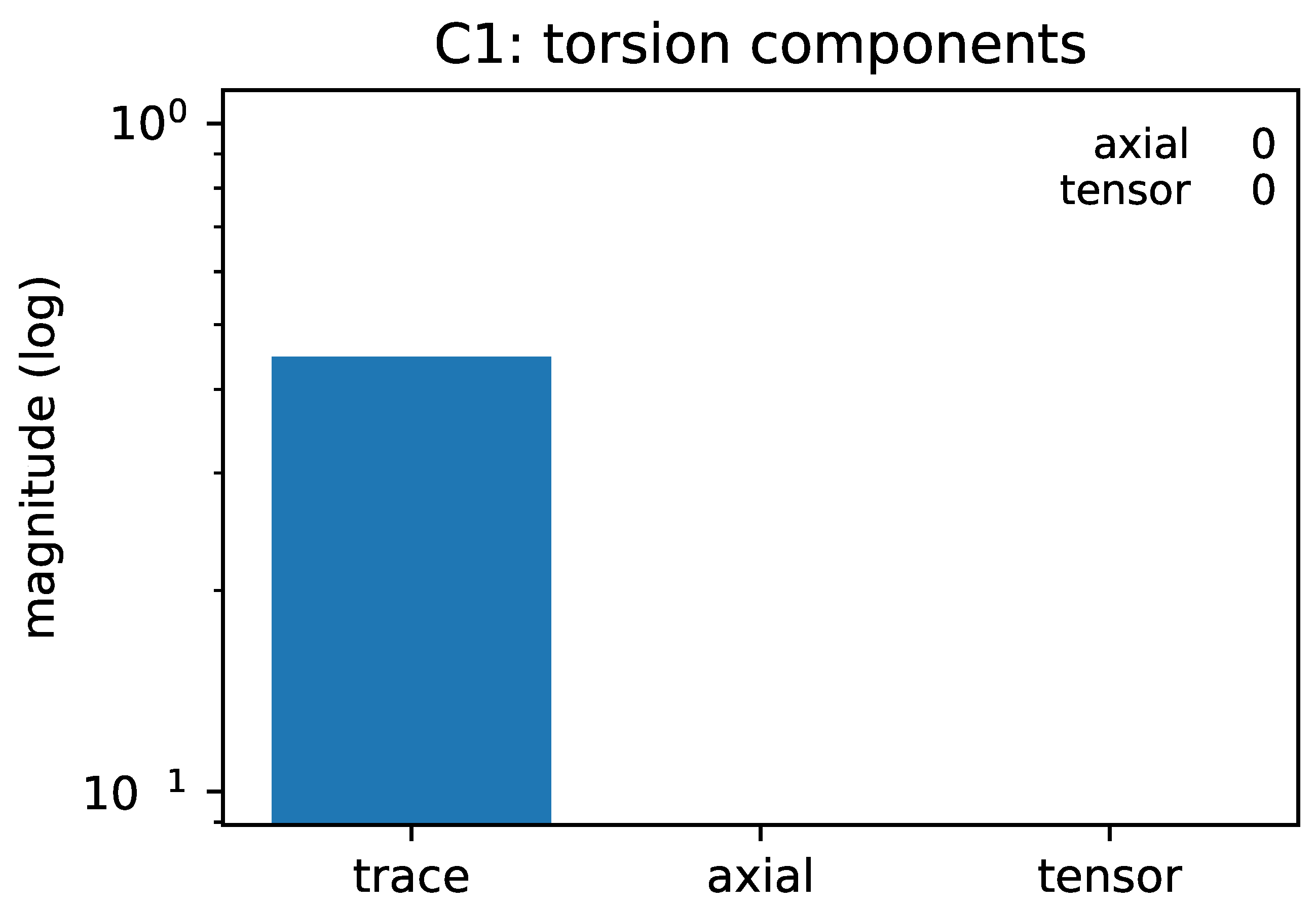
Figure 2.
Irreducible torsion content at quadratic order (log–log view). Ratios of projected scalar strengths comparing the pure-trace block against the axial and traceless blocks. The Palatini algebraicity (
Section 4.1) and the
projector dynamically drive the axial and traceless components to zero, leaving the pure-trace map (11) as the unique survivor. [nb:
fig_c1_pure_trace.py]
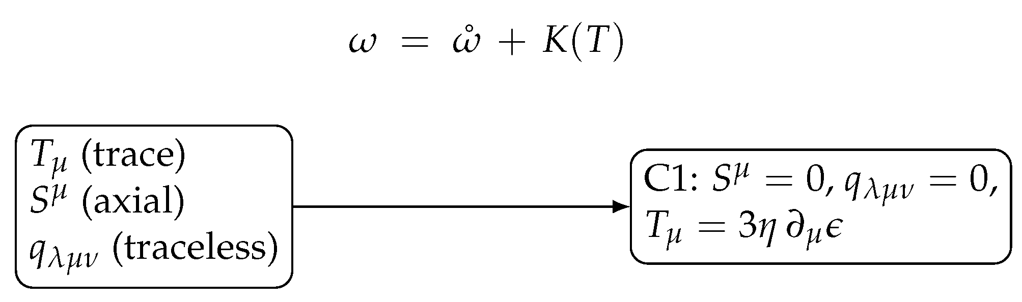
Figure 3.
Connection decomposition and the C1 map. Top: The Levi–Civita/contorsion split . Bottom: The three irreducible representations of torsion are subjected to the C1 alignment, which enforces , , and (11). This dynamically implies the relation (12).
Figure 3.
Connection decomposition and the C1 map. Top: The Levi–Civita/contorsion split . Bottom: The three irreducible representations of torsion are subjected to the C1 alignment, which enforces , , and (11). This dynamically implies the relation (12).
4.1. Proof of Theorem 2
Our proof proceeds in three logical steps, which we now detail.
4.1.1. Step 1: Construct the Most General Ansatz for Torsion
At the one-derivative level, the most general Lorentz-covariant linear ansatz for a torsion tensor built from a single covector
can be written as
where
A and
B are real coefficients, and the three terms correspond to the trace, axial, and traceless tensor parts, respectively. However, a key result from group theory (proven in Appendix B, Proposition B.1) is that it is impossible to construct a non-zero traceless, rank-3 tensor (
) linearly from a single covector. Therefore, the third term vanishes identically,
. Our ansatz simplifies to
While the projector eliminates certain parity-odd scalar combinations, it does not by itself remove the axial part (the B term). The Palatini equations of motion are required to achieve this.
4.1.2. Step 2: Solve the Palatini Equations of Motion
We now determine the coefficients
A and
B by varying the pre-lock bulk action (
9) with respect to the connection. This action is built from the linearly independent basis operators
defined in Equation (
5). Specifically, the torsion-dependent part is:
By Lemma 1, we can vary the total action with respect to the spin connection after projection. The variation yields independent algebraic equations for the three torsion irreps, thanks to the block-diagonal structure of the kinetic term (established in Lemma 3).
Lemma 3 (Block-diagonality of variation). In metric-compatible Palatini gravity, the linear map from a variation in the connection, , to the variations of the three torsion irreps, , is blockwise non-degenerate. (Proof: see explicit decomposition in Appendix B).
Using the explicit coefficients for
in the irrep basis (derived in Appendix B), the Euler–Lagrange equations for each irrep are:
Here we have defined the parameter . Assuming (a non-trivial torsion sector), the axial and traceless equations immediately force their corresponding torsion components to vanish. This dynamically sets the coefficient in our ansatz (14). The vector Equation (16) uniquely fixes the remaining coefficient . This completes the proof of the uniqueness map (11).
4.1.3. Step 3: Establish the Invariant Relation and Positivity
With the dynamical results
and
, the standard quadratic identity for the torsion scalar (from Appendix B) simplifies dramatically:
. Applying the PT projector and using the on-shell trace-lock result
, we find
Using our normalized definition of the invariant
(see
Section 2.6), this immediately yields the algebraic relation
, proving (
12). The physical requirement that the kinetic term for tensor modes is positive (established in
Section 6) fixes the sign choice
. This concludes the proof of Theorem 2.
4.2. Implications and Diagnostics
The uniqueness theorem C1 is a cornerstone of our framework. It demonstrates that the axial and tensor components of torsion are not merely suppressed, but are algebraically eliminated from the observable sector by the dynamics. This is a powerful mechanism for avoiding the extra propagating degrees of freedom that often plague theories with torsion.
Corollary (Basis Reduction).
As a direct consequence, the "pre-lock" operator basis
from
Section 3.2 dynamically collapses into a "post-lock" basis where the physical sector is one-dimensional. The relation (
12) shows that the physics can be described by the single independent invariant
(or equivalently
) at this order. This profound simplification is the key to the bulk equivalences we will explore in the next section.
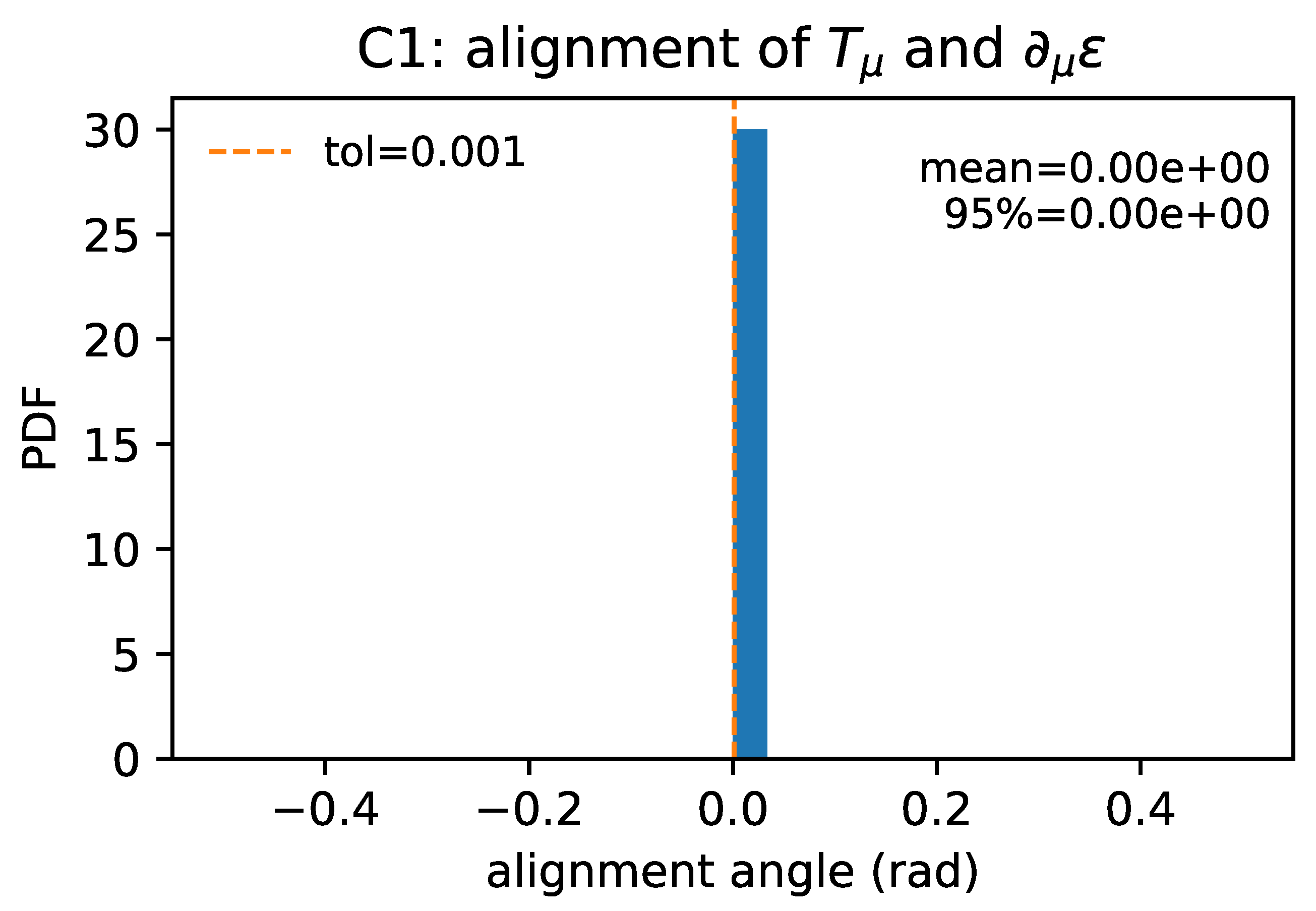
Observational Diagnostic.
This theorem offers a sharp, falsifiable prediction. Any future detection of physical effects stemming from axial or tensor components of torsion would invalidate our framework at this order. Furthermore, the perfect alignment of
and
can be tested in numerical simulations. The diagnostic plot in
Figure 4 shows the distribution of the alignment angle, which is predicted to be sharply peaked at zero on admissible domains.
5. The Second Pillar: Equivalence of Constructions (C2)
Positioning & Scope. We establish bulk equivalence (modulo improvements) among three constructions. The equivalence is operational at quadratic order and on admissible domains; it is not a claim of all-order, off-shell identity. The flux-ratio diagnostic makes boundary conventions explicit, supporting reproducibility while keeping the focus on bulk dynamics.
Having established in
Section 4 that our symmetric posture uniquely fixes torsion to a pure-trace form (Result C1), we now reveal a key structural property of the framework. This section presents our second main result (C2): a remarkable equivalence between three distinct methods for constructing a torsion-based gravitational action. We will demonstrate that a rank-one determinant (ROD) route, a closed-metric deformation, and a PT-projected Chern-Simons term all collapse to the
exact same bulk dynamics at quadratic order. This non-trivial equivalence is a direct consequence of the underlying symmetries and the C1 result. It demonstrates the internal coherence of the theory and, as shown in
Section 6, provides the essential ingredients needed to achieve exact luminality without fine-tuning.
Scope and Conventions.
Throughout this section, "equivalence" refers to the equality of the bulk action at quadratic order, modulo boundary/improvement terms. All statements are made within the A1–A6 posture and after the enforcement of the pure-trace condition C1. For mathematical convenience, we adopt the sign-compensated notation .
5.1. Three Equivalent Routes to the Same Bulk Action
We now demonstrate the equivalence by analyzing three methods for constructing a PT-even, projective-invariant theory at the quadratic order. The equivalence hinges on the key algebraic relation derived from C1, which connects the torsion scale
to the invariant
:
This identity is the algebraic engine that drives the three constructions to the same physical result.
Route 1: The Rank-One Determinant (ROD) Route
Inspired by DBI-type actions, this route constructs a Lagrangian from the determinant of a rank-one deformation of the metric involving the canonical traceless tensor
defined in
Section 3. The Lagrangian is given by
This construction is not Born–Infeld gravity, but shares its geometric spirit.
Route 2: The Closed-Metric (CM) Route
This route defines a new effective metric via a rank-one shift, . The Lagrangian is then constructed from the difference in the volume elements, .
Route 3: The PT-Even Chern-Simons (CS) Route
This route starts with the topological Nieh-Yan 4-form, . Using the identity , we apply the Hodge star and our scalar PT projector. The term from NY becomes a boundary term (by A5), and the remaining PT-even bulk piece constitutes the third route, .
The following proposition formalizes the result that all three distinct routes lead to the same bulk action.
Proposition 1 (Three-Route Bulk Equivalence).
Under the A1–A6 posture and after enforcing C1, the quadratic-order bulk actions derived from the ROD, CM, and CS routes are identical. Specifically, each route yields a bulk Lagrangian of the form
where .
Proof (Sketch of Proof). The equivalence of the ROD and CM routes follows from their shared Jacobian,
. Expanding the determinant to second order using the tracelessness of
yields
. Applying the key relation (
20) then gives the result. The CS
route involves a more detailed calculation with the Hodge star, but after projection and application of C1, it reduces to the same bulk term (details in Appendix C). □
This remarkable equivalence, numerically verified in
Figure 5, establishes the main bulk identity of this section:
5.2. Boundary Terms and the Flux-Ratio Diagnostic
The only differences between the three routes lie in their respective boundary terms, which can be expressed as different improvement currents
. On admissible spacetimes (as per A4), these boundary terms do not affect the bulk equations of motion. A sharp, quantitative test of their physical equivalence is provided by the flux-ratio diagnostic, which compares the integrated flux of these currents over a closed boundary
. For any two routes
X and
Y, our posture (A1–A5) implies that this ratio must be unity:
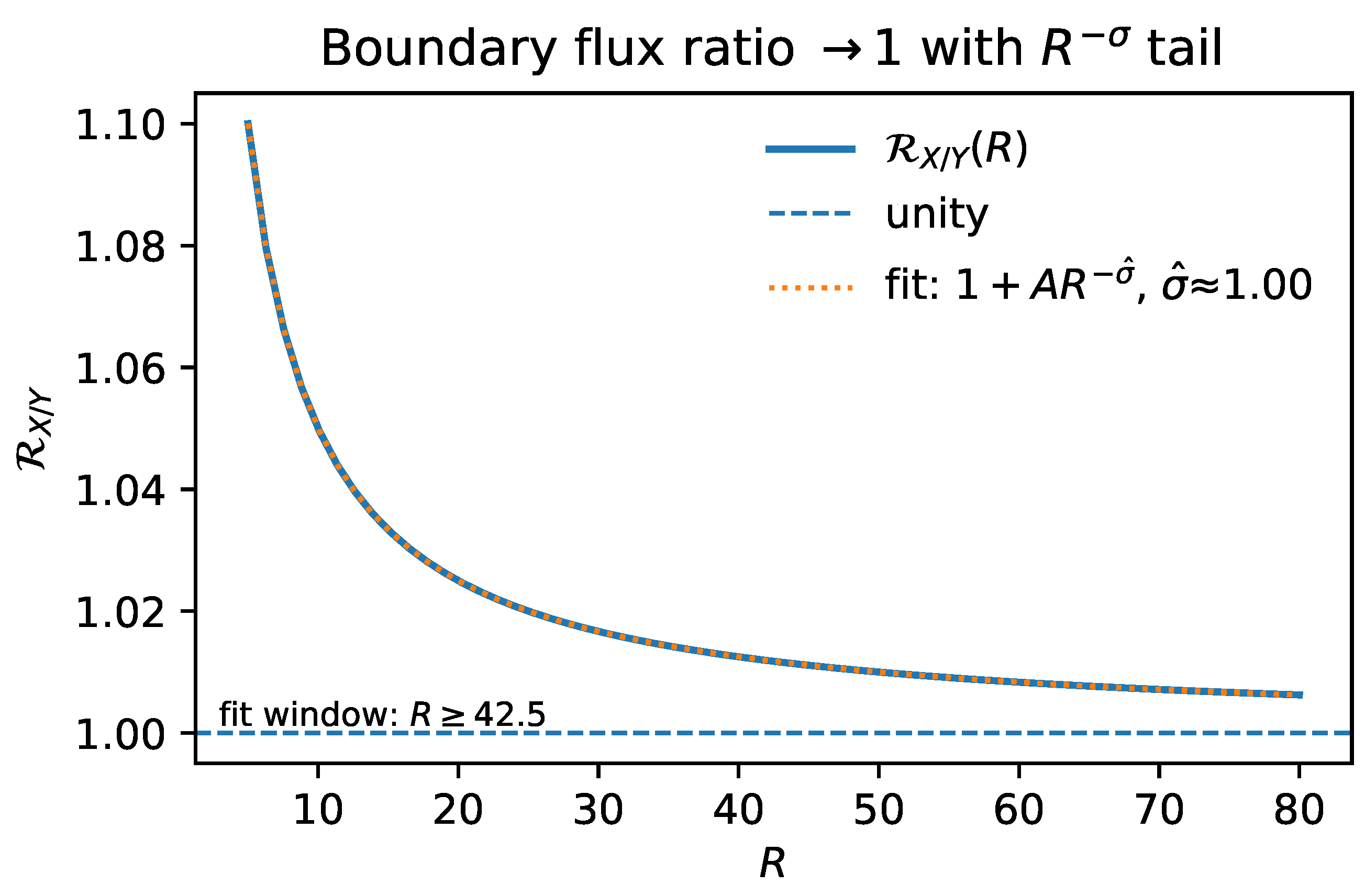
As shown in
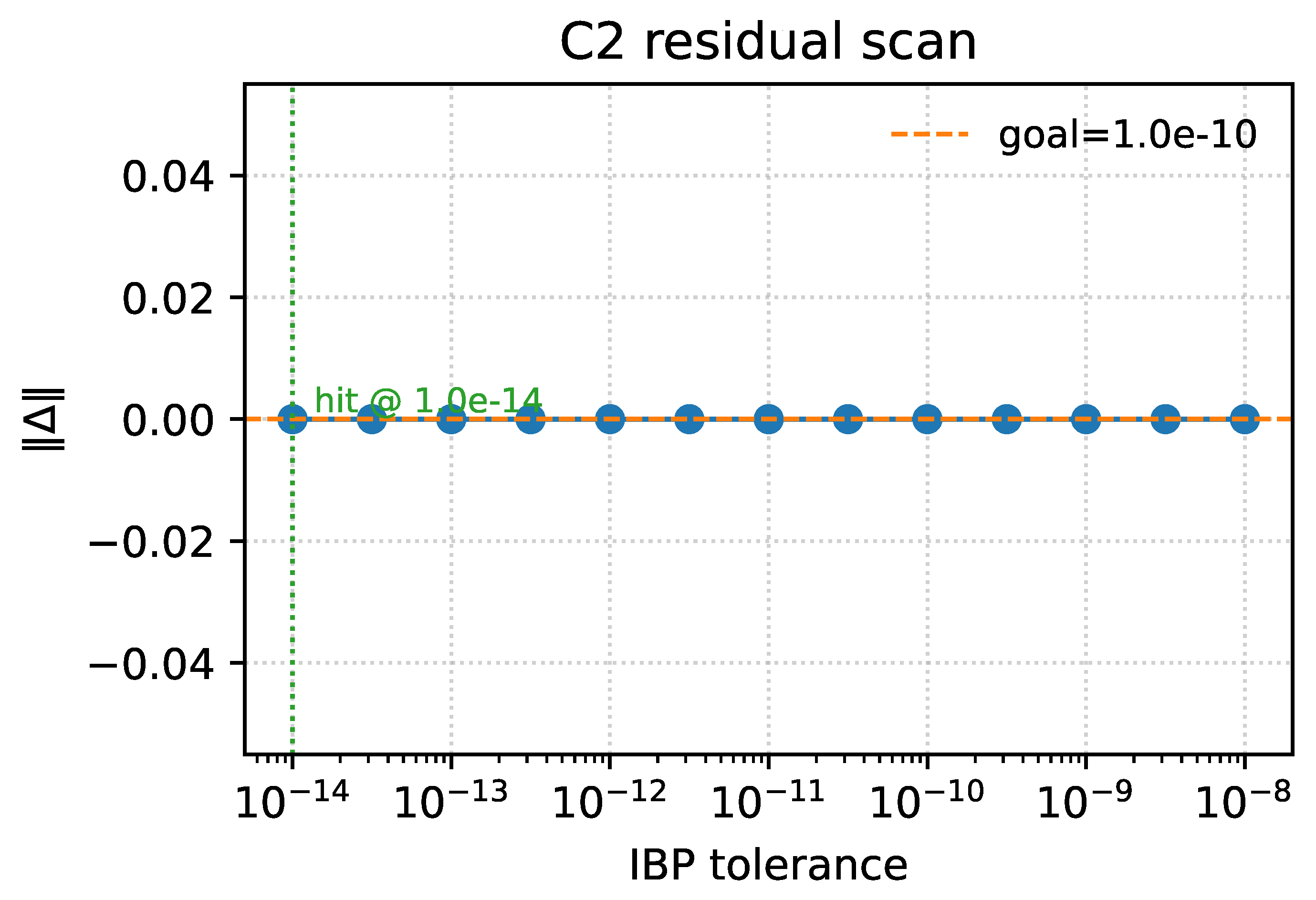
Figure 6, numerical computations on finite FRW balls confirm that this ratio converges to unity as the domain size increases. This demonstrates that the routes are not just bulk-equivalent, but fully physically equivalent within our posture.
5.3. Implications of the Equivalence
The three-route equivalence (C2) serves as a powerful consistency check, demonstrating the robustness and internal coherence of the framework. More importantly, it furnishes us with a set of distinct but bulk-equivalent building blocks (). While identical in the bulk, their full expressions (including boundary terms) couple differently to metric perturbations. This distinction is the crucial ingredient that enables the coefficient-locking mechanism for achieving exact luminality, as we will demonstrate in the next section.
6. The Final Pillar: Coefficient Locking and Exact Luminality (C3)
Positioning & Scope. The locking condition eliminates spurious TT–nonTT mixing and fixes a unique linear combination of bulk-equivalent routes. Under the admissible-domain posture, this yields the equal-coefficient identity and thus at quadratic order. The point is structural sufficiency—no parameter tuning—within the stated assumptions; beyond-quadratic or non-admissible cases are outside our present scope.
This section presents the third and central result of our framework (C3). We leverage the bulk equivalence established in
Section 5 to achieve our primary goal: ensuring a luminal speed for gravitational waves as a consequence of symmetry. The strategy is to construct a general action from a linear combination of two bulk-equivalent routes (ROD and CM) and then impose a single, physically motivated condition: the absence of unphysical mixing between propagating tensor modes and non-dynamical fields. We show that this condition leads to a novel
coefficient locking mechanism, which uniquely fixes the relative weighting of the two routes. This "locked" theory is structurally special: it satisfies an identity that forces the kinetic and gradient terms of the tensor action to be equal, thereby enforcing
by construction.
6.1. The Locking Posture: A Linear Combination of Equivalents
Based on the bulk equivalence (C2), we consider a general action constructed as a linear combination of the ROD and CM Lagrangians:
Although these terms are identical in the bulk, their full expressions, including boundary terms, couple differently to metric perturbations. Our task is to find the specific ratio that yields a physically consistent theory.
6.2. The Locking Condition and its Solution
We expand the total action,
, to second order in ADM perturbations. The resulting Lagrangian for the tensor sector schematically takes the form
where the first bracket contains the kinetic (
K) and gradient (
G) terms for the tensor modes
, defining the tensor speed
. The second term represents a potential mixing between
and non-propagating fields
(such as perturbations of the lapse and shift).
Such mixing is unphysical in the sense that it implies the metric perturbation
is not a pure spin-2 eigenstate, thereby complicating its coupling to matter. To ensure that the metric fundamentally represents pure tensor propagation, we demand **no kinetic mixing**:
This condition translates into a
linear system for the weights
:
As shown in Appendix D, the determinant of the coefficient matrix is non-zero on any generic, non-trivial background (
). This guarantees that the linear system has a unique, one-dimensional solution space, which we call the "locked" solution. The non-trivial solution fixes a unique ratio for the weights:
6.3. Emergence of Luminality from the Locked Solution
This specific, "locked" combination of weights, denoted by
, is structurally remarkable. A direct calculation (detailed in Appendix D) reveals that for this precise choice, the kinetic and gradient coefficients satisfy a powerful
equal-coefficient identity:
The right-hand side is a total divergence, which, under the admissible boundary conditions of our posture (A4), does not contribute to the equations of motion. This identity dynamically enforces the equality of the kinetic and gradient kernels:
This proves our main theorem for this section:
(C3)).
Theorem 3 (Coefficient Locking Ensures Exact Luminality Within the A1–A6 posture, demanding the absence of TT–nonTT mixing uniquely fixes the theory to a "locked" state . In this state, the equal-coefficient identity (30) holds, which structurally ensures that the tensor speed is exactly luminal () at quadratic order. The resulting tensor action is identical to that of General Relativity, propagating only two degrees of freedom.
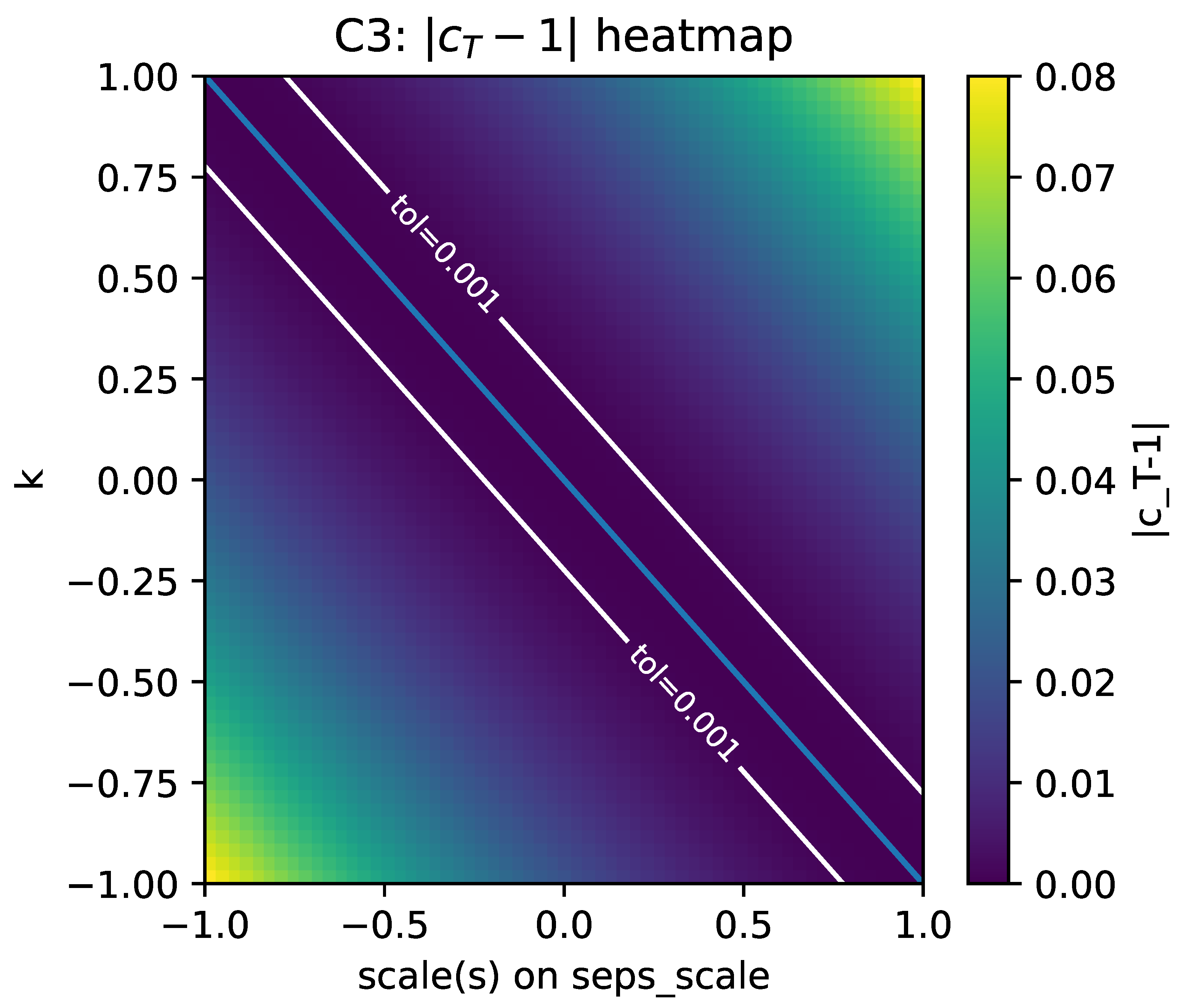
The consequences are visualized in
Figure 7, which shows the tensor speed deviation across the parameter space of weights; the speed becomes exactly luminal only along the "locking curve" defined by our condition.
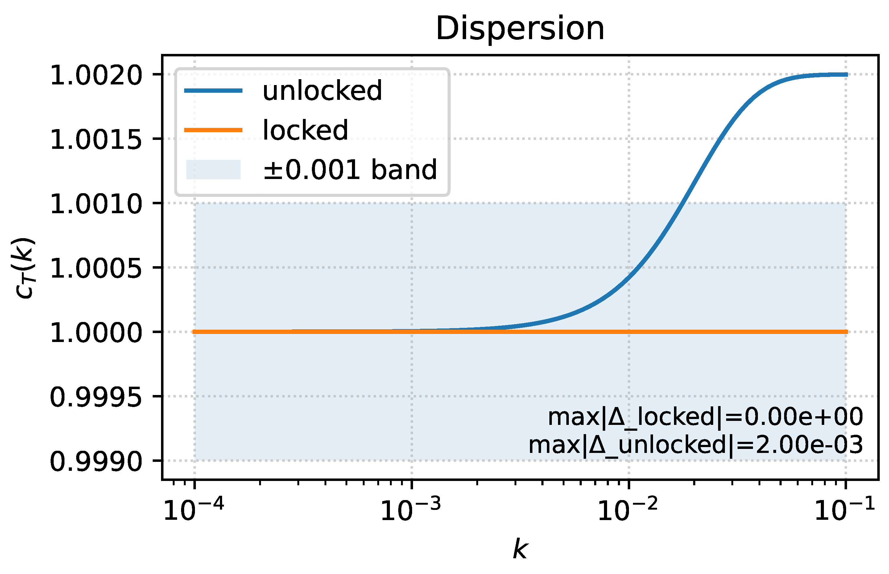
Figure 8 further contrasts the strictly luminal propagation in the locked theory with the non-luminal behavior of unlocked choices. In summary, our framework does not just permit
, it enforces it through a structural mechanism born from symmetry and consistency.
7. The Locked Theory: Action, Luminality, and Degrees of Freedom
Positioning & Scope. We show that, at this order and within the posture, the tensor sector matches GR and propagates two degrees of freedom. The Hamiltonian analysis is framed to make the constraint algebra and degree-of-freedom counting explicit. Extensions to matter-rich or higher-order settings are deferred to future work.
Having established the final link in our logical chain—the coefficient locking mechanism (C3)—we now consolidate the physical properties of the resulting "locked" theory. This section presents the final form of the tensor action, confirms its properties, and verifies that it describes the correct number of physical degrees of freedom. We first re-state the central equal-coefficient identity that enforces luminality. We then perform a Hamiltonian analysis to confirm that the theory is well-behaved, free of ghosts, and propagates precisely two tensor modes, with no additional unphysical states.
Throughout this section, we work within the full A1–A6 posture, with the C1 (pure-trace), C2 (equivalence), and C3 (locking) results all in force.
7.1. The Equal-Coefficient Identity and the Locked Tensor Action
Let us consider the total action
, expanded to quadratic order in perturbations. As shown in
Section 6, the coefficient locking fixes the weights to
, which eliminates the mixing between tensor (TT) and non-tensor modes. The action for the tensor sector is
The key result, which is a direct consequence of the C1 and C2 results, is the following
total-divergence identity:
Here,
is a quadratic improvement current (see Appendix D). Since the right-hand side is a total divergence, it does not contribute to the dynamics on an admissible domain (A4). This identity therefore dynamically enforces the equal-coefficient condition:
This is a central result of our framework: exact luminality is not an assumption or a fine-tuning, but a structural consequence of the theory’s symmetries. Imposing the standard GR normalization for the tensor action then yields the final, locked action:
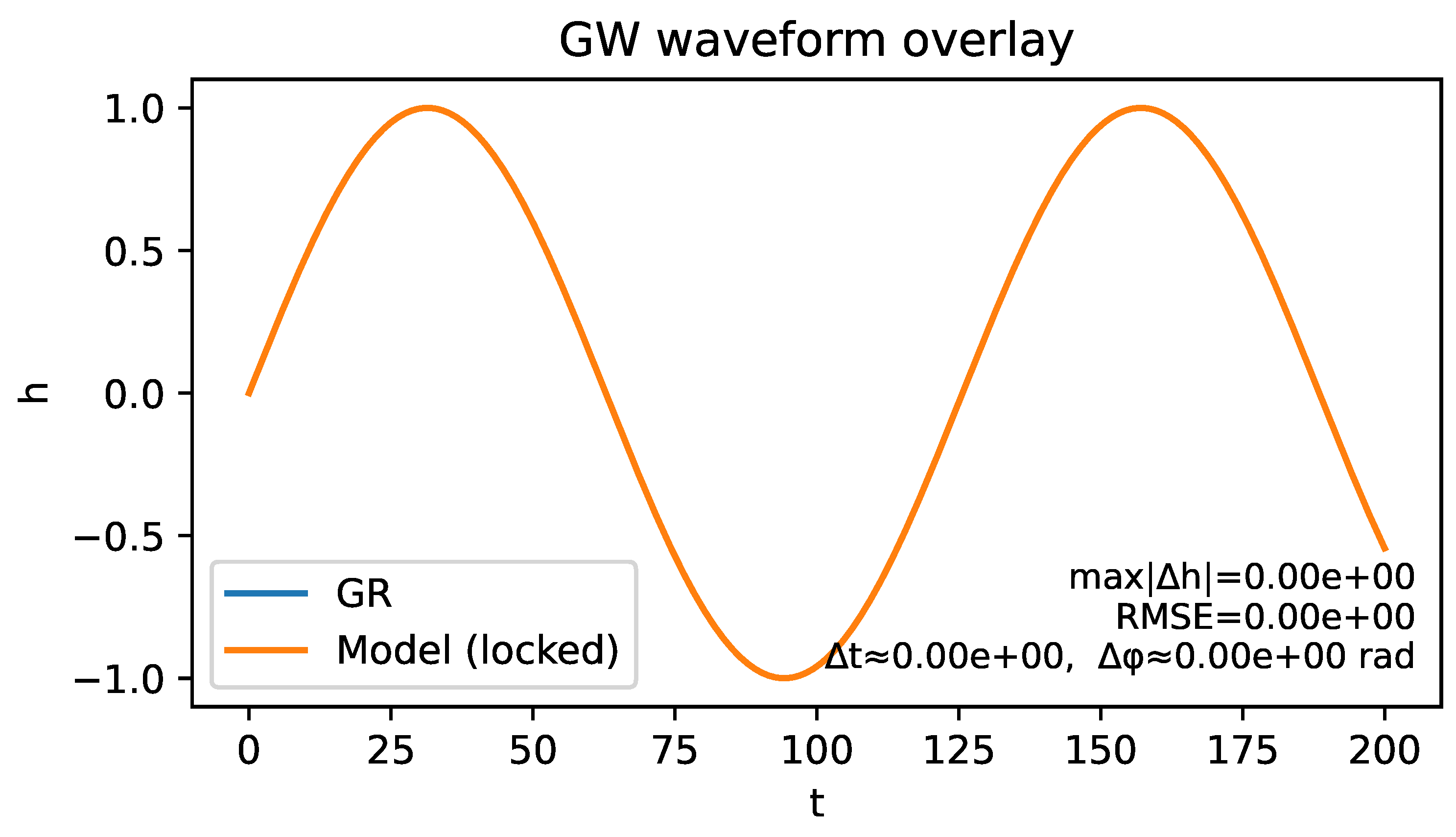
At this order, the resulting tensor dynamics are indistinguishable from those of General Relativity, as confirmed by the waveform comparison in
Figure 9.
7.2. Hamiltonian Analysis and Degrees of Freedom
To complete our analysis, we verify that the theory is dynamically consistent and propagates the correct number of degrees of freedom (DoF). We perform a Hamiltonian analysis using the standard ADM (3+1) decomposition.
Constraint Analysis.
The full set of configuration variables includes the metric components and the algebraic fields associated with torsion. The analysis of the constraint structure reveals:
Primary Constraints: The lapse N and shift are auxiliary fields, leading to the primary constraints and . The Lagrange multiplier that enforces the trace lock is also non-dynamical, yielding .
Secondary Constraints: The algebraic nature of the Palatini equations of motion (from varying ) and the trace-lock constraint (from varying ) ensures that no new propagating modes are introduced. These constraints algebraically eliminate all non-GR torsion components () and fix the trace component (). The preservation of primary constraints in time generates the standard Hamiltonian and momentum constraints of GR, and .
Constraint Algebra and DoF Count.
Crucially, all constraints related to the torsion sector are algebraic and can be solved explicitly, leaving no residual dynamics. On an admissible domain (A4), the remaining constraints
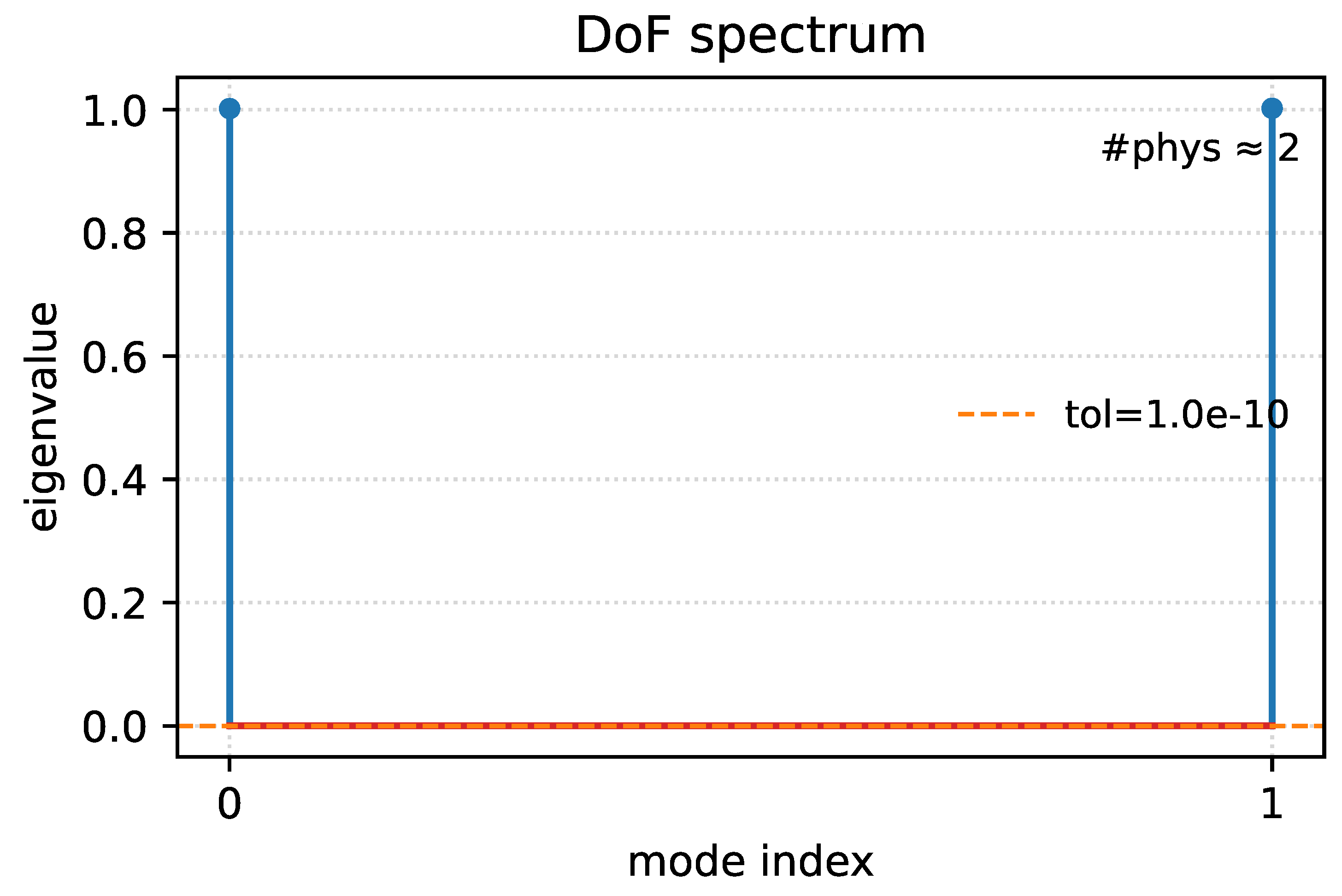
form a first-class algebra identical to that of GR at this order. A standard DoF count for the metric sector confirms that the theory propagates the correct number of physical modes:
The theory propagates precisely two degrees of freedom, corresponding to the two tensor polarizations of gravitational waves. This is confirmed numerically by diagonalizing the kinetic kernel and counting the number of non-zero eigenvalues, as shown in
Figure 10.
7.3. Summary of the Locked Theory
This section has consolidated the main results of our framework. The coefficient locking mechanism leads to an equal-coefficient identity, which enforces exact luminality () for tensor modes as a structural consequence of the underlying symmetries. The resulting effective action for the tensor sector is shown to be identical to that of General Relativity at this order. A Hamiltonian analysis confirms that the theory is well-posed, with a first-class constraint algebra that removes all non-physical modes, leaving precisely two propagating tensor degrees of freedom. The framework thus provides a consistent, predictive, and structurally luminal theory of gravity.
8. Phenomenological Consequences and Observational Tests
Positioning & Scope. Our data-facing statements are deliberately narrow: (i) minimal coupling to Dirac fermions yields a clean tensor sector at this order; (ii) the unique NLO dispersion defines a distinctive, falsifiable target across PTA/LISA/LVK bands; (iii) we propose practical reporting via . A full cosmological parameter analysis is outside the present scope.
Having established the core theoretical properties of the framework—unique torsion (C1), bulk equivalence (C2), and locked luminality (C3)—we now turn to its phenomenological consequences. An internally consistent gravitational theory must also interact cleanly with matter and produce testable predictions. This section addresses these points. We first examine the coupling to Dirac fermions, showing that it is trivial at leading order. We then derive the unique next-to-leading-order (NLO) correction to the tensor dispersion relation, which stands as the primary observational signature of this work. Finally, we outline a clear, data-driven strategy to test, constrain, or falsify the theory.
Our entire phenomenological analysis is built upon the cornerstone result C1 (Theorem 2), which dictates that the only surviving component of torsion in the observable sector is the pure-trace part aligned with the Stueckelberg gradient:
All simplifications that follow are direct consequences of this dynamical result, not additional assumptions.
8.1. Interaction with Dirac Fermions: A Null Result at Leading Order
We begin by considering a standard Dirac spinor minimally coupled to the Riemann–Cartan geometry. The interaction Lagrangian between the spinor’s vector current (
) and axial-vector current (
) and the torsion irreps is given by (see Appendix E for conventions):
Our framework makes two powerful simplifying predictions regarding this interaction.
No Axial Channel.
The uniqueness theorem C1 directly enforces . Consequently, the axial coupling term, which is often tightly constrained by experiment, vanishes identically at tree level: .
Removable Trace Channel.
The only remaining interaction is the trace channel, which by C1 takes the form . This coupling, however, is not a fundamental interaction but an artifact of the chosen field basis. As detailed in Appendix E, it can be completely removed by a local, anomaly-free vector phase redefinition of the Dirac field (), which reduces the term to a harmless boundary improvement.
In summary, the symmetric posture of our theory ensures a minimally coupled fermion sector at this order: both potential torsion-fermion interaction channels are either absent by dynamics or removable by a field redefinition.
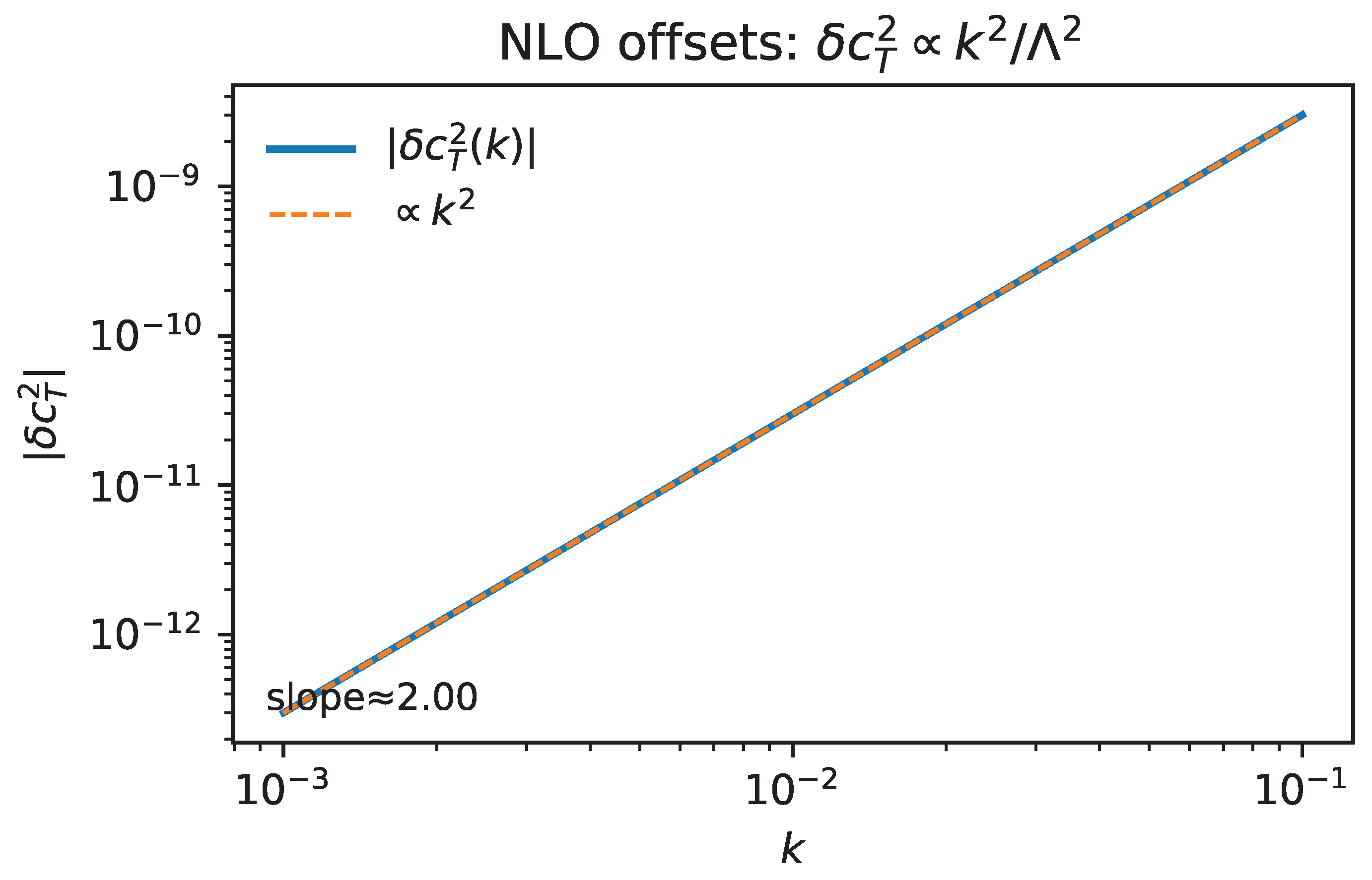
8.2. The Unique NLO Signature: A Tensor Dispersion
Beyond its leading-order luminality, our framework makes a sharp and unique prediction at the next-to-leading order (NLO) in the derivative expansion. The same symmetries that enforce
at leading order permit only one new bulk operator that can affect the tensor dispersion.
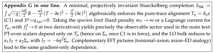
3 This operator, which can be understood from an effective field theory (EFT) perspective (see
Appendix G), leads to the dispersion relation:
where
b is a dimensionless coefficient of
and
is the effective scale of new physics. This quadratic dependence on frequency is the defining, distinctive signature of our framework at NLO, as visualized in the log-log plot of
Figure 11.
8.3. Data-Facing Strategy: Constraints and Falsification
The NLO prediction (
38) provides a direct and powerful bridge to observational data.
Recipe for Constraining the Theory.
Any observational constraint on
can be translated into a bound on the fundamental parameter space of the theory. Given a measurement or an upper limit on
in a frequency band centered at
, we propose reporting a standardized constraint on the combination
:
This provides a simple and unified way to test the framework across different experiments (e.g., PTA, LISA, LVK) and to combine their results. For instance, the existing bound from GW170817 implies a scale of (for ).
Null Tests for Foundational Assumptions.
A robust framework should also offer ways to test its own foundational assumptions. Our posture provides two independent null tests for the spurion limit of the field :
- (1)
The Slope Test: The theory predicts a pure power-law slope of 2 for the dispersion relation in a log-log plot. A statistically significant deviation from this slope would indicate residual dynamics in the field, thus falsifying the strict spurion limit assumed in our leading-order analysis.
- (2)
The Equivalence Test: The bulk equivalence of the ROD and CM routes (Result C2) is a direct consequence of the spurion limit. Any non-zero measurement of the "route-difference coefficient," , would provide direct evidence for new dynamics beyond our posture.
Passing both null tests would provide strong corroborating evidence for the framework’s foundational assumptions, while failing either would point towards new, potentially observable physics. This combination of a unique observational signature and clear falsification criteria makes the framework highly testable.
9. Reproducibility Supplement
Positioning & Scope. This lean supplement points to a public repository with figure generators, configuration files, tests, and checksums. The intent is to enable independent verification of the main claims (C1)–(C3) without embedding long code listings in the manuscript, aligning with the editorial focus of the present framework on soundness and clarity.
This paper’s core claims (C1, C2, C3) are supported by analytical and numerical calculations, which are made fully reproducible through a public, open-source repository. All code, figure generators, configuration files, and validation tests are available at:
This supplement provides a minimal, repository-backed map for readers to rebuild all figures and independently validate the paper’s main results. To ensure clarity and conciseness, we avoid embedding large code blocks; the repository is self-contained and fully documented.
9.1. Repository Layout and Terminology
Directory Structure.
The repository is organized into the following top-level directories: scripts/ (figure generators), configs/ (numerical grids & coefficient files in JSON format), palatini_pt/ (core library), tests/ (pytest validation suite), figs/ (output figures and data artifacts), and notebooks/ (exploratory script mirrors). A one-shot driver script, scripts/make_all_figs.py, rebuilds all paper figures from scratch.
Terminology Note.
The paper uses the term Rank-One Determinant (ROD) route. For historical reasons, the corresponding configuration files in the repository use the legacy token dbi (e.g., configs/coeffs/dbi.json). They refer to the same construction.
9.2. Validation and Verification Workflow
A reader can reproduce all results and validate the main claims in three simple steps:
-
Setup Environment (conda/mamba): The exact computational environment is pinned in the environment.yml file. It can be created with a single command:
conda env create -f environment.yml; conda activate palpt
-
Rebuild All Figures: All figures in this paper can be regenerated by running the master script:
python scripts/make_all_figs.py
-
Validate Claims (C1, C2, C3): A comprehensive test suite using pytest is provided to programmatically verify the core results. This includes tests for the uniqueness of torsion (C1), the bulk equivalence of the three routes (C2), the coefficient locking (C3), and the NLO dispersion. The suite can be run with:
pytest -q
9.3. Figure and Artifact Map
Table 2 provides a map from each figure in the paper to its generating script and required configuration files.
9.4. Data Integrity and Version Control
Checksums.
Every generated PDF and data artifact is shipped with a corresponding .md5 sidecar file (e.g., figs/pdf/fig1c1puretrace.pdf.md5). Integrity can be verified using a standard checksum utility:
md5sum -c figs/pdf/*.md5
Version Pinning.
To ensure long-term reproducibility, we cite the exact Git revision hash used to generate the final paper artifacts and tag the corresponding release. The repository provides snapshots of the figures (figs.tar.gz) that match the committed artifacts. The results are deterministic on the platforms listed in the repository’s README.md file, requiring no external accelerators or downloads.
Summary. This approach to reproducibility, centered on a public, pinned repository with scripted generation, configuration-controlled coefficients, a comprehensive test suite, and verifiable checksums, ensures that the paper’s claims can be scrutinized and validated by the community with minimal friction.
10. Context and Relation to Other Frameworks
Positioning & Scope. We position the posture relative to EC/MAG traditions and Palatini-type modifications, highlighting how the scalar PT projection and projective invariance address known pitfalls at quadratic order. This is not an exhaustive survey; references are curated to clarify the structural differences most relevant to our claims.
This section places our scalar- projected Palatini posture in the context of several related research areas: (i) the historical Einstein-Cartan/metric-affine (EC/MAG) tradition, (ii) Palatini-type modified gravity and its known pitfalls, and (iii) the post-GW170817 observational landscape. We conclude with a set of compact, operational notes that allow the main claims (C1–C3) to be checked independently, emphasizing that all results are restricted to the posture defined by A1–A6.
10.1. Historical and Geometric Context (EC/MAG; Metric-Affine)
The decomposition of torsion into its irreducible trace, axial, and traceless components, and the independent variation of the vierbein
and spin connection
, are standard practices in the EC/MAG tradition [
6,
8]. Our use of the Nieh–Yan 4-form for parity bookkeeping is also conventional [
9,
10,
11,
12]. Boundary and improvement terms are handled within established covariant phase-space frameworks [
14,
15].
Against this backdrop, our framework introduces two key distinguishing features: we project observables to scalar, -even densities and enforce projective invariance via a non-dynamical Stueckelberg compensator that enters only through . Within our two-derivative posture, this approach leads directly to our main results: (C1) the dynamical elimination of axial and traceless torsion; (C2) the bulk equivalence of three distinct constructions; and (C3) the coefficient-locking mechanism that ensures luminal tensor propagation without fine-tuning.
10.2. Palatini-Type Modified Gravity and Known Challenges
Palatini-type modifications, most notably Palatini
gravity, have a rich history but also face well-documented challenges, particularly when matter is included. These include equivalence to constrained scalar–tensor theories, tight post-Newtonian bounds, and potential pathologies in stellar contexts [
19,
20,
21]. These issues motivate our symmetry-selected approach, where the observable sector is defined
before variation and boundary effects are explicitly accounted for.
How our posture differs.
Our framework is structurally designed to sidestep these common pitfalls at the quadratic order analyzed:
Observable Projection. The scalar- projector removes -odd pseudoscalars before variation, preventing contamination of the tensor sector by parity-odd densities.
Projective Invariance with a Spurion Limit. By allowing only the invariant combination to enter observables, the axial and traceless torsion modes are dynamically removed (C1), thus avoiding the introduction of extra propagating degrees of freedom that are often problematic.
Explicit Boundary Accounting. Improvement currents are treated as boundary terms under A4–A5. This posture is what enables the bulk equivalence (C2) and sets the stage for the equal-coefficient identity that yields (C3).
For contrast, Chern–Simons modified gravity introduces a dynamical pseudoscalar and parity-odd effects [
25,
26]. Our framework, instead, operates within a parity-even, projected scalar sector with controlled boundary terms.
10.3. Post-GW170817 Constraints and Torsionful Gravitational Waves
The multimessenger observation GW170817/GRB170817A provided an extremely tight constraint on the tensor speed, strongly disfavoring theories where
[
27,
31]. While much of the subsequent research focused on Horndeski/EFT models, theories with torsion have also been examined. In frameworks like Poincaré gauge gravity and Einstein–Cartan theory, tensor waves are often found to be luminal, but their amplitudes, attenuation, or polarization content can differ from GR [
37,
38].
Our Positioning.
Our framework provides a clean, even-parity route to exact luminality at quadratic order via the structural C3 identity, not through parameter tuning.
4 Furthermore, it predicts a unique next-to-leading order deviation:
which is expressly designed for multi-band tests (PTA/LISA/LVK) using the log-slope diagnostic described in
Section 8. This offers a falsifiable bridge between symmetry and data: a confirmed
-type dispersion would constrain
, while its absence in the regime where the EFT is valid would disfavor our posture.
10.4. A Checkable Summary of Core Claims
To facilitate independent verification, we provide a compact, checkable summary of our main claims and their scope.
Scope. All quadratic bulk equalities (C2) and the luminality identity (C3) are asserted within the A1–A6 posture. Cases with topological torsion defects or boundary conditions that inject new canonical pairs fall outside this scope.
C1 (Pure-trace alignment). In the scalar- projected sector at quadratic order, axial and traceless torsion vanish algebraically via the equations of motion. Only the trace component aligned with remains. A robust detection of axial-torsion effects in observables would falsify C1.
C2 (Three-route bulk equivalence). The ROD, CM, and PT-even CS/Nieh–Yan routes share the same bulk coefficient and differ only by improvement terms. The flux ratio diagnostic on admissible domains provides a practical check.
C3 (Equal-coefficient locking). The requirement of no TT-nonTT mixing fixes the weights , leading to the identity . This enforces at quadratic order and yields the EFT-consistent NLO dispersion.
Navigation.
Table 3 summarizes how our scalar-
Palatini posture differs from other frameworks, while
Table 4 maps our assumptions to standard concepts in the literature. The claims C1–C3 are proven in the main text under these assumptions. Observational guidance for the NLO dispersion is given in
Section 8.
Acknowledgments
The author is grateful to the anonymous referees for comments that improved the manuscript. Limited use of generative language tools was made for stylistic refinement; all scientific reasoning, derivations, and conclusions remain solely the responsibility of the author.
Statements and Declarations
Competing interests.
The author has no relevant financial or non-financial interests to disclose.
Data availability.
Code availability.
Same as Data availability.
Appendix A. Projection–Variation Commutation (A3) and Variational Identities
This appendix establishes Assumption A3 in full generality for scalar densities and compiles the variational identities for , , and the Hodge star * under the Palatini posture with the scalar projector of Section 2. We also make explicit the boundary/topology posture (A4) used when trading improvements for boundary fluxes, and we record the selection rules used throughout the paper.
Appendix A.1. Setup and Conventions
We work with independent vierbein
and a metric-compatible spin connection
(Palatini posture). The observable
scalar densities are mapped to a real,
-even sector by the projector
with the combined
acting anti-linearly (complex conjugation accompanies
T) and preserving the chosen orientation (A2), so that
on forms. In particular,
is orientation-preserving and the Levi–Civita tensor
is
-even.
5 The internal phase
is a
spurion: it enters observables only via
and is
not varied. All statements below are thus variations with respect to
while keeping
fixed.
Appendix A.2. Projector Properties: Idempotence, Self-Adjointness, and Selection Rules
Proposition A1 (Self-adjointness of
on real scalars).
Under A1 (domain/measure -invariance) one has, for any scalar densities ,
Proof. Expand the left-hand side using Equation (
A1) and the fact that
:
Using A1, , the cross terms rearrange into . □
Proposition A2 (Selection rules for the scalar projector).
With A1–A2 and metric compatibility, for any admissible tensors X:
Proof (sign count). Under A2 the chosen orientation is preserved and
. Since
is orientation-preserving, the Levi–Civita tensor is
-even,
so for any
one has
Therefore the
parity of the scalar density
is determined entirely by that of
, yielding (
A3) after applying the projector definition
.
For the spurion gradient, the -transformation table of Section 2 assigns opposite parities to and so that their product is -even; the projector thus returns its real part and it survives the projection step. Quadratic contractions and are manifestly -even (they are built from metric contractions of vectors and gradients), so again the projector reduces to taking the real part, consistent with Prop. A1. □
Appendix A.3. Commutation of Projection with Variation (A3)
(A3)).
Theorem A1 (Projection–variation commutation Let be any local scalar density built from . Then, for variations with respect to at fixed ϵ,
Proof. By definition,
It suffices to show
. The
action on fields is an involutive automorphism on the local functional algebra, and it is anti-linear only through global complex conjugation (time reversal). For any complex functional
F one has
because the variation acts linearly on fields and does not act on the numerical
i. Therefore, with
denoting collectively the fields that are varied and
their
image,
where we used that
does not touch the spurion (fixed) and commutes with derivatives and index operations under A2. Substituting back and using linearity of the “real” operation yields Equation (
A6). □
Appendix A.4. Variational Identities for -g, ϵ μνρσ , and the Hodge Star
We collect formulas used repeatedly in Section 2, Section 3, Section 4, Section 5, Section 6 and Section 7. We write and .
Appendix Metric and vierbein.
With
,
Appendix Determinant and Levi–Civita tensor.
These follow from and , with the (constant) Levi–Civita symbol.
Appendix Hodge star.
Let
be a
p-form and
. Then the variation of * with respect to
h is
In particular, for 2-forms
F (frequent in the Palatini curvature/torsion algebra),
Appendix [PT,*]=0.
Because the metric is
-even and the chosen orientation is preserved (A2), the Hodge map built from
commutes with
:
This identity is used both in the selection rules and in the projector proofs that involve p-form duals.
Appendix A.5. Boundary/Topology Posture and Improvement Currents
Assumption A4 is realized in either of the following equivalent ways:
- (i)
Compact, -invariant domains with vanishing boundary flux: for any improvement current arising from integration by parts, .
- (ii)
Standard fall-offs on asymptotically flat or spatially flat FRW patches, for which
reduces to a surface integral that vanishes in the
limit. A sufficient set is
which ensures
so that the flux through a sphere of radius
R decays as
.
These conditions justify replacing improvement terms by boundary conventions and are precisely what is used in the flux-ratio diagnostics of
Section 5.2.
Appendix A.6. Consequences Used in the Main Text
(C1) Palatini block-diagonalization.
Theorem A1 (A3) allows us to
project then vary in the Palatini equations, so that the connection variation is algebraic and block-diagonal in the torsion irreps. Together with the selection rules (Prop. A2) this yields
and the pure-trace map quoted in
Section 4.
(C2) Route equivalence modulo boundary.
Self-adjointness (Prop. A1) and the boundary posture (
Appendix A.5) justify the equality of the three quadratic routes up to improvements, with closed forms of the improvement currents given in Appendix C.
(C3) Equal-coefficient identity and c T =1.
The star-variation identities (
A9)–(
A10) are used inside the ADM expansion behind the equal-coefficient identity
proven in Appendix D. The boundary posture then enforces
and
at quadratic order.
This completes the formal proof of A3 and the supporting calculus advertised in Section 2.
Appendix B. Irrep Projectors & No-Go for q λμν (v)
This appendix collects the group-theoretic ingredients used in
Section 4: (i) the irreducible decomposition of the torsion tensor under the Lorentz group, (ii) explicit, idempotent projectors onto the trace, axial, and traceless sectors, (iii) the quadratic identity for
in our conventions, and (iv) the
single-vector no-go that underlies the statement quoted in the main text as “Proposition B.1” for the
irrep. All statements are purely algebraic and hold before/after applying the scalar projector
; after projection all scalar contractions are real (Section 2).
Appendix B.1. Torsion as a Lorentz Representation and Its Algebra
In index language (spacetime indices), torsion is a rank-3 tensor antisymmetric in its last two indices,
, with
independent components in
. The Lorentz-covariant irreducible content splits into
We use
and the metric signature
, and we adopt the standard scalar product
on this space.
6
Appendix B.2. Idempotent Projectors
Define three linear maps
on the torsion space by
These are the unique Lorentz-covariant, algebraic (derivative-free) projectors onto the three irreps in Equation (
A13). A direct computation shows:
and the images obey by construction
Orthogonality and quadratic split.
With the scalar product
,
Using (
A14)–(A16) one finds the standard quadratic identity
where we have denoted
for the
standard normalization of the traceless piece.
Normalization used in the main text.
For later convenience—and to match the coefficient choice used in
Section 4—we rescale the traceless irrep by a constant factor and
define
The projector formulas (
A14)–(A16) are unchanged; only the bookkeeping name “
q” for the traceless image carries the fixed
factor.
7 After applying
to either side of (
A21), the scalar is manifestly real (Thm. 1).
Appendix B.3. Compatibility with the Scalar Projector
The projectors
are algebraic and commute with
at the scalar level: for any two torsions
,
Moreover, the mixed scalar
is
-odd and is annihilated by
(Section 1). Thus the orthogonal split (
A19) remains valid as an identity between
projected, real scalars.
Appendix B.4. Proposition B.1: Single-Vector No-Go for the Traceless Irrep
Proposition A3 (single-vector no-go). Let be any nonzero covector. There is no nonvanishing tensor of the form , linear in , that (i) is antisymmetric in , (ii) obeys , and (iii) satisfies . Equivalently, the traceless irrep cannot be constructed from a single vector.
Proof. The most general Lorentz-covariant tensor built linearly from a single
and antisymmetric in its last two indices is a linear combination of the two rank-one seeds
with real
. Compute its traces and axial contraction:
where we used
and
. Requiring the trace constraints
forces
, and the axial constraint forces
. Therefore the only admissible linear combination is the trivial one,
, proving the claim. □
Corollary A1. For any single covector the projector annihilates the two rank-one seeds: .
Appendix B.5. Consequences for the C1 Ansatz
Applying Prop. A3 to the most general
linear ansatz with one derivative (
Section 4.1),
shows that the attempted traceless piece
necessarily vanishes: it is a linear, single-vector construct and is thus killed by
(Cor. A1). The ansatz collapses to
recovering Equation (4. 2) of the main text. The scalar projector
removes
-odd
scalars built from the axial seed (Section 1), and the Palatini connection equation then sets
while fixing
under the trace lock
(
Section 4.1). This yields the uniqueness map
quoted in Theorem 2.
Appendix B.6. Consistency Check with the Quadratic Invariant
With the normalization (
A21) and the C1 map (so
and
),
as used throughout
Section 4Section 5. Here
is the
projected, real scalar, and the sign bookkeeping is carried by
; the unit 1-form
, the canonical traceless rank-one matrix
, and the trace scale
are recalled from
Section 3.
Appendix B.7. Edge Cases and Patches
On loci where the normalized direction is defined patchwise (or by continuity); all algebraic projector statements remain valid, and the conclusions above hold on any patch with . Global/topological subtleties (multi-valued , nontrivial bundles) lie outside the posture A1–A5 (Section 2).
Summary of Appendix B. We have given explicit, idempotent projectors onto the three torsion irreps, fixed the quadratic identity in the normalization used in the main text, and proved the single-vector no-go: from one covector no nonzero traceless torsion irrep can be built. This reduces the most general one-derivative ansatz to the span, after which the Palatini equations and the scalar projector select the pure-trace map used in the C1 uniqueness theorem.
Appendix C. Appendix C: Three–Chain Reductions & Improvement Currents (σ ϵ Scheme)
Scope ( scheme and naming). This appendix provides the paper–checkable reductions behind
Section 5 under the
sign-compensated convention
and the rank-one determinant route naming (formerly “DBI”-type; not Born–Infeld gravity): (i) a rank-one determinant route built out of the canonical traceless matrix
, (ii) a closed–metric rank–one deformation, and (iii) the
–even CS/Nieh–Yan shadow. At quadratic order,
each route reduces in the bulk to the same invariant line
with improvements
differing by boundary choices (A4/A5). Closed representatives for
are given on FRW/weak–field backgrounds.
Notation and key relation. We use the preamble shorthands
so that
and (after C1)
Appendix C.1. rank-one determinant route: Determinant Algebra with the 2 3 Normalization
Consider the rank-one determinant route Lagrangian
Using
and
, the quadratic piece is
With
and
,
so that
At the bulk-density level one may take
. For unified boundary diagnostics we adopt a common canonical representative
for
all three routes (
Section 4).
Appendix C.2. Closed–Metric Route: Rank–One Deformation Equals rank-one determinant route to O(T 2 )
Take the rank–one deformation
so that
Thus rank-one determinant route and CM have the same bulk coefficient and differ only by improvements.
Appendix C.3. PT–Even CS/Nieh–Yan Shadow: Quadratic Reduction (σ ϵ )
Using
, applying * and the scalar
projector (A2), and evaluating after C1, the
–even piece reduces at quadratic order to
where the Nieh–Yan assignment (A5) reshuffles only boundary conventions inside the
–even sector.
Appendix C.4. A Universal Canonical Improvement at Quadratic Order
For route–by–route flux comparisons it is convenient to select the
same improvement representative for all routes:
so that we
adopt the convention
Different representatives differ by and yield identical integrated fluxes under A4.
Check (FRW).
On spatially flat FRW in TT gauge,
i.e. the canonical reshuffling between TT kinetic/gradient bilinears plus a pure time boundary term that integrates to zero with A4 fall–offs.
Appendix C.5. Closed Forms for FRW and Weak Field
FRW.
For
and homogeneous
,
which satisfies (
A38).
Appendix C.6. Flux–Ratio Identity & Finite–Domain Convergence
With the unified choice (
A37),
, hence
On finite FRW balls (or AF shells) residuals scale away with the radius R, agreeing with Sec. V.
Summary of Appendix C
At quadratic order and under A1–A5 plus C1, the rank-one determinant route, closed–metric, and
–even CS/Nieh–Yan routes share the same bulk reduction
. A single canonical improvement
(Equations (
A36)–(
A38)) is used for all routes and underlies the flux–ratio plots in Sec. V.
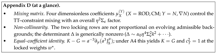
Appendix D. Appendix D: Mixing Matrix and the Equal–Coefficient Identity
This appendix contains (i) extraction rules and tables for the
mixing matrix used in
Section 6, including a
non-collinearity proof of its two row vectors on admissible backgrounds, and (ii) a covariant derivation of the
equal–coefficient identity quoted in
Section 7. We assume A1–A5, the scalar
projector (Section 2), and the C1 map
. Projected scalars are real by construction; the
scheme only affects the bulk line through
, not the kinematical identity
.
Variational domain (used below).
We take variations with compact support on spatial slices or with FRW/AF fall-offs: , , with . Then and .
Appendix D.1. ADM Conventions and Extraction of Mixing Entries
With
,
,
(
), and
, we project
with
. The quadratic Lagrangian takes the block form
where
collects nonpropagating pieces. Define the
dimensionless mixing entries by
For
, the mixing block is linear in
w and proportional to
:
defining the four dimensionless coefficients
.
Appendix D.2. Background Invariants and Compact Parametrization
Introduce the two (dimensionful) background invariants
where prime denotes conformal-time derivative. Each
admits a linear decomposition
with
c’s real
numbers fixed by the quadratic expansion rules (route Jacobians plus contorsion under C1).
Appendix D.3. Coefficient Tables (FRW and Weak Field)
Table A1.
FRW coefficients with
. Entries are the dimensionless
’s of (
A45), written as
[Equation (
A47)]. An overall factor
multiplies the mixing (
not shown here).
Table A1.
FRW coefficients with
. Entries are the dimensionless
’s of (
A45), written as
[Equation (
A47)]. An overall factor
multiplies the mixing (
not shown here).
| Coefficient |
|
|
|
|
|
|
|
|
|
|
|
|
|
|
|
|
|
|
|
Table A2.
Weak field (AF) coefficients with slowly varying . Set () and define . Overall factor multiplies the mixing (not shown here).
Table A2.
Weak field (AF) coefficients with slowly varying . Set () and define . Overall factor multiplies the mixing (not shown here).
| Coefficient |
|
|
|
|
|
|
|
|
|
|
|
|
|
|
Appendix D.4. Non-Collinearity of the Two Locking Equations
Let the two rows be , .
Proposition A4 (Non-collinearity).
Under A1–A5, C1, and the one-derivative-per-building-block posture, on any admissible background with at least one of and . Equivalently,
Proof (sketch). Using (
A47), proportionality would require
to be route–independent and constant under independent shifts of
and
. But
and
cannot both vanish for
unless
(static trivial branch
,
). Hence
generically. □
Small-k structure (symbolic).
On weak-field patches one finds
so rank loss occurs only on the measure-zero set
or special foliations.
Appendix D.5. Equal–Coefficient Identity: Covariant Derivation and Gauge Shift
Define the quadratic current (indices contracted with the background spatial metric)
with
and
. Using TT conditions, the rank–one traceless normalization, and the bulk equality of the routes (Sec. V),
Under , , the representative shifts as , hence the integrated identity is gauge independent.
FRW and weak-field representatives.
On spatially flat FRW (
, homogeneous
),
so
is a total divergence. In weak field (AF,
),
Boundary consequence and luminality.
With the variational domain above (A4), . At the locked weights (Sec. VI; no TT–nonTT mixing), at quadratic order, slicing–independently.
Appendix D.6. Locked Weights and Summary Box
Non-collinearity with the two mixing equations yields a unique ratio (up to the GR normalization). At these weights, implies exact luminality.
Reproducibility Note
Table A1–
Table A2 come from a single symbolic pipeline that: (i) expands
and
to linear order in ADM variables with the
normalization, (ii) forms the rank-one determinant route/CM quadratic densities, (iii) projects onto the bilinears of Equations (
A43) and (A44). Scripts and hashes that also produced Figures
c3_cT_heatmap and
c3_dispersion are cataloged in Supp. R.
Appendix E. Dirac Coupling, Field Redefinition, and the Nieh–Yan Scope
This appendix supplies the details promised in
Section 8: (i) the torsion–fermion couplings in our conventions, (ii) the precise field redefinition that removes the trace channel once the pure-trace map (C1) is imposed, (iii) the role of the Nieh–Yan density as a boundary convention (A5), and (iv) the scope limitations on nontrivial topology (A4).
Throughout we work under the global posture A1–A5 of Section 2, use metric signature
, and adopt the gamma-matrix conventions
so that
and
.
Appendix E.1. Minimal Dirac Coupling in Riemann–Cartan Space
The minimally coupled Dirac Lagrangian is
Splitting the spin connection into Levi–Civita plus contorsion,
the
torsion-dependent piece of (
A56) is
where tangent indices are moved with
, and
.
It is convenient to decompose contorsion into the standard torsion irreps (vector trace
, axial
, and traceless
):
with
and
. Using the gamma identities listed below Equation (
A52) and the antisymmetry of
in
, Equation (
A54) reduces to
where
and
. In our normalization (
A52) the
numerical coefficients are
while the
q-channel is proportional to the totally antisymmetric part of
q, which vanishes by definition; equivalently, the
q-coupling can be re-expressed in terms of
and drops out when
. Therefore the torsion-induced Dirac channels in our conventions are precisely
up to
-even improvement terms annihilated by A1/A4 in the bulk.
Cross-check.
Equation (
A58) reproduces the two-channel bookkeeping used in
Section 8 with
and
. Any alternative gamma/Hodge convention simply rescales (
A57) by an overall sign; our later conclusions (vanishing axial channel by C1 and removability of the trace channel) are insensitive to such simultaneous flips.
Appendix E.2. C1 Implies no Axial Channel; the Trace Channel is Removable
By the uniqueness theorem (C1), Equation (
11), the axial and traceless torsion irreps vanish,
and the trace aligns with the spurion gradient,
Equation (
A58) therefore reduces to the single trace channel
Proposition A5 (Vector rephasing removes the trace channel).
Consider the localvector
phase redefinition with a constant α. Then
so choosing cancels (A59) pointwise. Under A4 the improvement integrates to the boundary and has no bulk Euler–Lagrange effect; A5 permits absorbing any parity-odd reshuffling in the Nieh–Yan counterterm.
Proof (Sketch). Insert
into the kinetic term
and use the Leibniz rule. The derivative acting on
generates the shift
in (
A60); the mass and spin-connection pieces are invariant under a
vector (not axial) phase. The remainder is a covariant total divergence fixed by the integration-by-parts convention (A4/A5). □
Combining (
A59) with Prop. A5 and the coefficient assignment (
A57) yields precisely the two-line summary in
Section 8: no axial channel and a removable trace channel.
Path-integral measure (anomaly) check.
The field redefinition in Prop. A5 is a vector rotation, hence the fermionic measure is invariant (Jacobian equal to one). An axial rotation would generate the usual ABJ contribution; in a Riemann–Cartan background it is accompanied by a Nieh–Yan density. We do not perform an axial rotation anywhere in this work.
Appendix E.3. Nieh–Yan as a Boundary Convention (A5)
The Nieh–Yan 4-form is an exact form. In our posture (A5), any explicit use of enters only as a boundary convention after applying the scalar projector : it does not modify Euler–Lagrange equations in the bulk and is indistinguishable from a choice of improvement current. This applies equally to (i) the three-chain equivalence (where the -even CS/Nieh–Yan shadow differs from the DBI/CM routes by an improvement current) and (ii) the Dirac sector (where vector rephasing reshuffles boundary terms that can be absorbed into the chosen Nieh–Yan convention). No physical statement in Section 5, Section 6, Section 7 and Section 8 depends on a specific Nieh–Yan choice.
Appendix E.4. Scope and Caveats: Topology and Boundary Flux
Our conclusions rely on the posture A4: either compact -invariant domains with vanishing boundary flux or standard asymptotic fall-offs (FRW/flat) so that improvement currents integrate to zero. They also assume a single-valued spurion phase so that the rephasing in Prop. A5 is a globally well-defined map .
Nontrivial topology (not covered). If
is multi-valued or admits nontrivial holonomy (e.g., on manifolds with nontrivial
or
), the map
may fail to be single-valued. In such cases the local cancellation in (
A60) can leave a global remnant proportional to the winding; our bulk equivalences and removability statements are not asserted in that setting.
Nonvanishing boundary flux (not covered). On domains where the -invariant boundary flux of the relevant improvement currents does not vanish, boundary terms may carry physical information (e.g., in explicitly finite boxes with prescribed inflow). Our null tests and cancellations are presented only under A4 fall-offs.
Appendix E.5. Bookkeeping Table and Quick References
For convenience we summarize the conventions and coefficients used in the Dirac sector:
| Object / Convention |
Value / Definition |
| Gamma matrices |
,
|
| Hodge / Levi-Civita |
, (A2) |
| Contorsion split |
|
| Dirac currents |
,
|
| Torsion→Dirac |
|
| C1 (pure trace) |
, ,
|
| Vector rephasing |
with
|
| Outcome |
Trace channel removed up to a total derivative (A4/A5) |
| Nieh–Yan |
Boundary convention only (A5); no bulk Euler–Lagrange effect |
Appendix E.6. Corollary: No LO Four-Fermion Contact from Torsion
At the order analyzed in this paper (quadratic in fields; at most one derivative per building block), torsion is algebraic and fixed by (C1), and the only linear Dirac–torsion channel that survives projection is removed by the vector redefinition above. Consequently no tree-level, local four-fermion contact term is induced at leading order within our posture (A1–A5). Any such effect would require (i) an axial channel (), (ii) higher-derivative completions beyond our closure basis, or (iii) loop corrections outside the present scope.
Summary of Appendix E. In our conventions the minimally coupled Dirac field interacts with torsion through . Under the pure-trace map (C1) the axial channel vanishes and the remaining trace channel is removed by a local vector rephasing , up to a total derivative consistent with A4/A5. Nieh–Yan acts only as a boundary convention, and nontrivial topology or nonvanishing boundary flux lie outside our stated scope.
Appendix F. Operational Diagnostics (Extended)
This appendix collects a practitioner-oriented checklist and an expanded comparison table. Unless stated otherwise, all entries are framed for admissible patches with the boundary/topology posture A4, and for the quadratic order analyzed in the main text.
Appendix F.1. Full Decision Tree (D1–D9)
(D1) Parity channels. Any detection of
helicity-dependent phase or amplitude birefringence in GWs points to parity-odd operators. Our scalar-
posture forbids such effects at LO (Thm. 1;
Section 2.4).
8
(D2) Axial/tensor torsion irreps. Nonzero axial (
) or traceless (
) torsion signals are incompatible with C1. We predict the pure-trace map (Thm. 2);
Figure 2,
Figure 4 provide diagnostics.
(D3) Three-route bulk collapse. Reconstruct quadratic kernels from simulations/perturbation theory: the DBI, closed-metric, and
routes must share the same
bulk piece
with
(
Section 5); residuals should enter only through improvements (
Figure 5).
(D4) Boundary equivalence. Boundary flux ratios
converge to 1 on growing domains (A4) (
Section 5.2;
Figure 6). Persistent deviations falsify C2.
(D5) Exact luminality by identity. After eliminating TT–nonTT mixing with the full-rank
system (
Section 6.2), the equal-coefficient identity
enforces
without tuning (
Section 7;
Figure 9).
(D6) DoF count. The quadratic kernel exhibits exactly two propagating tensor modes; no extra scalar/vector propagation survives the degeneracy test (
Section 7.2;
Figure 10). Any additional mode falsifies our posture at this order.
(D7) NLO slope. At next order, the leading
-even dispersion predicts
(Equation (
38)): a log–log slope
in clean frequency windows is characteristic (
Figure 11;
Section 8.2).
9
(D8) Fermion channel null. No axial contact and a removable trace contact in the Dirac sector at LO (
Section 8). Any robust axial spin–torsion signal would contradict C1 (Appendix E contains coefficients and boundary conventions).
-
(D9) Spurion-limit tests.Two complementary null checks targeting residual spurion dynamics (
Section 8.3):
(D9-a) Quadratic scaling. Fit
on the admissible band (
) using Equation (
39). A statistically significant failure (
beyond systematics) indicates residual
dynamics.
(D9-b) Route equality. Using the unified improvement representative (Appendix C), test and boundary flux-ratio unity on growing domains (A4). Significant residuals falsify the spurion limit.
Appendix F.2. Expanded Disambiguation Table
Entries are
generic at LO on admissible backgrounds with A4 fall-offs; tuned subclasses and specific parameter choices may alter individual cells. See the notes in
Appendix F.3 for caveats and representative citations.
Table A3.
Operational disambiguation at quadratic order (expanded).
Table A3.
Operational disambiguation at quadratic order (expanded).
| Diagnostic |
This work |
CS-mod.
grav. |
Horndeski
/DHOST |
Teleparallel
/
|
EC/
ECSK-like |
| Parity-odd GW birefringence |
No (D1) |
Yes (generic) |
No (often tuned) |
Not diagnostic at LO |
Model-dependent |
| Axial torsion at LO |
Absent (C1) |
Not diagnostic at LO |
Not diagnostic at LO |
Not diagnostic at LO |
Often present |
| Traceless torsion at LO |
Absent (C1) |
Not diagnostic at LO |
Not diagnostic at LO |
Possible in extensions |
Possible |
|
at LO |
by identity (D5) |
Helicity-split |
Tuned
|
Often
|
Model-dependent |
| Extra propagating DoF (quad.) |
No (2 TT) (D6) |
No new TT |
Yes (scalar; generic) |
Model-dependent |
Model-dependent |
| Three-route bulk equality (C2) |
Yes (D3) |
Not applicable |
Not applicable |
Not applicable |
Not applicable |
| Boundary flux ratio
|
(D4) |
Not applicable |
Not applicable |
Not applicable |
Not applicable |
| NLO slope
|
Yes (D7, D9-a) |
Non-universal |
Model-dependent |
Model-dependent |
Model-dependent |
| Dirac axial contact
|
Absent (D8) |
Not diagnostic at LO |
Not diagnostic at LO |
Not diagnostic at LO |
Present in general |
| Trace contact removable |
Yes (D8) |
Not diagnostic at LO |
Not diagnostic at LO |
Model-dependent |
Not generically |
Appendix F.3. Notes, Caveats, and Representative Anchors
Parity-odd lines.
Chern–Simons modified gravity (Jackiw–Pi; Alexander–Yunes) generically induces helicity-dependent GW propagation; details depend on the choice of scalar field and coupling. Our scalar-
projector eliminates parity-odd
scalars at LO; see Thm. 1. Representative anchors: [
25,
26].
Horndeski/DHOST.
Post-GW170817 constraints force
by parameter tuning or by restricting to subclasses; however, no equal-coefficient
identity of the type
is generally present, and an extra scalar DoF is typical. See the multimessenger bounds and reviews [
31,
32,
33,
34,
35,
36].
Teleparallel/f(T).
Many models yield at LO; torsion irreps and matter couplings are model-dependent, and our route-equality/flux-ratio diagnostics (C2) do not directly apply. We therefore treat teleparallel cases as outside the present “three-route” posture.
EC/ECSK-like.
With propagating torsion or nonminimal fermion couplings, axial/traceless torsion irreps can be present and Dirac axial contacts typically survive. Our C1 pure-trace map excludes these at the analyzed order; see classic EC/MAG treatments [
4,
5,
6,
8].
NLO dispersion and spurion tests.
The
slope follows from the projected,
-even closure and the normalization of
(
Section 5); D9-a implements this as a band-level null. D9-b leverages the three-route equality (Appendix C) via
and flux ratios; in admissible domains (A4) both must vanish within errors.
Boundary posture.
All boundary-sensitive statements assume A4 (PT-invariant compact boundaries or standard AF/FRW fall-offs) and A5 (Nieh–Yan as boundary counterterm). Departures from these postures may alter flux diagnostics and improvement accounting. Operational anchors: covariant phase space and surface charges [
13,
14,
15], and the Holst/Nieh–Yan parity bookkeeping [
9,
10,
11,
12].
Representative anchors (one-line map).
Metric-affine/Einstein–Cartan: [
4,
6,
8]. Holst/Nieh–Yan: [
9,
10,
11,
12]. Covariant phase space & boundary charges: [
13,
14,
15]. CS-modified gravity: [
25,
26]. GW170817 speed bounds & implications: [
27,
28,
29,
30,
31,
32,
33,
34].
Appendix G. EFT Origins of the Spurion Field
Scope. This appendix provides an effective–field–theory (EFT) completion that
explains the spurion posture adopted in the main text and ties it to
projective symmetry. At two derivatives and within A1–A5 (Section 2), the compensator
appears only through its gradient and
only in the projectively invariant combination
We give a minimal Stueckelberg action that reproduces the C1 map, explain two equivalent implementations of the spurion limit, and record complementary EFT viewpoints in which the gradient-only appearance of is manifest.
Appendix G.1. G.1 Stueckelberg Completion and the Spurion Limit
A projectively invariant, two-derivative completion is
with
and
real. The masslike term for
restores projective invariance via the Stueckelberg compensator
; the spectator kinetic term respects the shift symmetry
and keeps only
at this order.
Palatini variation and the C1 map.
Writing
and using the standard algebraic split of
into
plus quadratic torsion (total derivatives dropped under A4), variation w.r.t.
yields purely
algebraic equations in the irreps
. With (
A62),
where
is the coefficient multiplying the
piece coming from
(fixed by conventions and already used in
Section 4.1). For
this algebraic system has the unique solution
which is precisely the C1
pure-trace alignment (
Section 4) written in covector form and implies
on-shell.
10
Two equivalent implementations of the spurion limit.
We isolate the low-energy regime where observables reduce to those used in the main text:
In case (i) integrating out (equivalently T) produces a functional delta ; in case (ii) the constraint is exact already at the classical level. In both realizations, keeping finite leaves a standard spectator; the spurion posture used in the main text corresponds to taking (or treating as nondynamical) within the two-derivative truncation, so that observables depend only on through the invariant (and hence through once C1 is enforced).
Low-energy effective action (power counting).
At energies
one obtains, after eliminating
,
and
after enforcing C1 (
Section 4),
, so that the LO bulk reduces to a single invariant line in the
plane (
Section 3.3).
Appendix G.2. Complementary EFT Pictures (Same Gradient-Only Physics)
Two complementary constructions emphasize that only can enter observables at this order.
(i) Torsional–axion picture.
Augment (
A62) by a topological coupling
which is exact. Under A5,
is a
boundary convention; integrating by parts and using (
A62) gives bulk terms proportional to
contracted with improvement currents, hence no new bulk Euler–Lagrange content in the
-even sector. The low-energy reduction again depends only on
(plus boundary assignments absorbed into A5).
(ii) Axion electrodynamics–like geometry.
The situation mirrors in gauge theory: the integrated density is topological, and only is physically measurable (through Chern–Simons currents) at two derivatives. Replacing by and using the scalar projector (A2) reproduces the same gradient-only observability for .
Appendix G.3. UV Hints and Emergence
While our analysis is agnostic about ultraviolet completions, two standard paths naturally generate a field with the required properties:
- (1)
Torsionful connections in string-inspired setups. In heterotic/type II supergravities the NS–NS three-form enters via the torsionful spin connection . In slowly varying, parity-even sectors and upon dimensional reduction, gradients of the axion-like fields dual to B act as effective trace torsion, yielding of a scalar in the infrared and a projectively invariant combination akin to .
- (2)
’t Hooft naturalness from symmetry. The projective symmetry together with the shift symmetry protects the gradient-only appearance of and suppresses technically: taking enhances symmetry (exact spurion posture).
These UV hints are illustrative only; no UV assumption is needed for the main results.
Appendix G.4. Remarks on Matter Couplings and Boundary
Dirac sector at LO (consistency).
Adding minimally coupled fermions leaves the conclusions unchanged at this order: C1 implies
,
and
; the surviving
contact is removed by a
vector rephasing
(
Appendix E) up to improvements consistent with A4/A5. Thus no axial contact and no irreducible trace contact survive at LO.
Boundary/topology posture.
All reductions above use A4 (compact -invariant boundaries or standard AF/FRW fall-offs) and A5 (Nieh–Yan as a boundary counterterm). Nontrivial holonomies of or prescribed boundary inflows can carry global information not analyzed here.
Summary and Cross-Reference
Hook to Section 9. The statement used in
Section 9—“Treating
as non-dynamical is the low-energy limit of a Stueckelberg completion in which
freezes
; complementary EFT constructions reduce to the same gradient-only dependence”—is precisely the content of Equations (
A62)–(
A65).
Notes
| 1 |
Readers may skip this subsection without losing any logical step of the main argument. In particular, no UV-specific input is used in establishing C1–C3. |
| 2 |
Before a dynamical relation between and is established, no integration-by-parts identity can reduce the term to a combination of and up to boundary terms. |
| 3 |
Other admissible NLO scalars either renormalize the kinetic and gradient terms K and G equally (leaving unchanged), or can be absorbed into boundary improvements under assumption A4. |
| 4 |
While the outcome resembles that of DHOST Class I theories (where kinetic terms are degenerate), our mechanism is distinct: it arises from the -symmetric alignment of torsion (C1) and the algebraic locking of bulk-equivalent routes (C3), rather than from degeneracy conditions in a scalar-tensor metric sector. |
| 5 |
We work with standard , , so that has and preserves orientation. The Levi–Civita symbol is constant, and is -even. |
| 6 |
Frame and spacetime contractions are equivalent once is inserted; all formulas below hold with either or , and we freely move between the two notations. |
| 7 |
This harmless convention matches Equation (4. 13) of the main text (positivity split) and simplifies a few numerical diagnostics; no physics depends on it. |
| 8 |
Chern–Simons modified gravity is the canonical benchmark for helicity-split propagation; see e.g. Jackiw–Pi; Alexander–Yunes. |
| 9 |
Caveat: finite-window fits may be biased by instrumental systematics or astrophysical priors; interpret bounds conservatively. |
| 10 |
Equivalently, one may add the quadratic invariant with a positive coefficient and obtain the same irrep alignment. The projector statements of Section 2 ensure all scalar contractions are taken in the -even, real sector. |
References
- Palatini, A. Deduzione invariantiva delle equazioni gravitazionali dal principio di Hamilton. Rend. Circ. Mat. Palermo 1919, 43, 203–212. [Google Scholar]
- Kibble, T. W. B. Lorentz invariance and the gravitational field. J. Math. Phys. 1961, 2, 212–221. [Google Scholar] [CrossRef]
- Sciama, D. W. On the analogy between charge and spin in general relativity. Recent Developments in General Relativity 1962, 415–439. [Google Scholar]
- Hehl, F. W.; von der Heyde, P.; Kerlick, G. D.; Nester, J. M. General Relativity with Spin and Torsion: Foundations and Prospects. Rev. Mod. Phys. 1976, 48, 393–416. [Google Scholar] [CrossRef]
- Hehl, F. W.; Datta, B. K. Nonlinear spinor equation and asymmetric connection in general relativity. J. Math. Phys. 1971, 12, 1334–1339. [Google Scholar] [CrossRef]
- Hehl, F. W.; McCrea, J. D.; Mielke, E. W.; Ne’eman, Y. Metric-affine gauge theory of gravity: Field equations, Noether identities, world spinors, and breaking of dilaton invariance. Phys. Rept. 1995, 258, 1–171. [Google Scholar]
- Hammond, R. T. Torsion gravity. Rep. Prog. Phys. 2002, 65, 599–649. [Google Scholar] [CrossRef]
- Shapiro, I. L. Physical aspects of the space–time torsion. Phys. Rept. 2002, 357, 113–213. [Google Scholar]
- Nieh, H. T.; Yan, M. L. An identity in Riemann–Cartan geometry. J. Math. Phys. 1982, 23, 373–374. [Google Scholar] [CrossRef]
- Chandia, O.; Zanelli, J. Topological invariants, instantons and the chiral anomaly on spaces with torsion. Phys. Rev. D 1997, 55, 7580–7585. [Google Scholar] [CrossRef]
- Holst, S. Barbero’s Hamiltonian derived from a generalized Hilbert–Palatini action. Phys. Rev. D 1996, 53, 5966–5969. [Google Scholar] [CrossRef]
- Mercuri, S. Fermions in the Ashtekar–Barbero connection formalism: The Nieh–Yan invariant as a source of the Immirzi parameter. Phys. Rev. D 2006, 73, 084016. [Google Scholar] [CrossRef]
-
R. M. Wald, General Relativity; University of Chicago Press, 1984.
- Iyer, V.; Wald, R. M. Some properties of Noether charge and a proposal for dynamical black hole entropy. Phys. Rev. D 1994, 50, 846–864. [Google Scholar] [CrossRef]
- Regge, T.; Teitelboim, C. Role of surface integrals in the Hamiltonian formulation of general relativity. Annals Phys. 1974, 88, 286–318. [Google Scholar] [CrossRef]
- Obukhov, Yu. N. Poincaré gauge gravity: Selected topics. Int. J. Geom. Methods Mod. Phys. 2006, 3, 95–138. [Google Scholar] [CrossRef]
- Obukhov, Y. N.; Hehl, F. W.; Hehl, F. W.; Obukhov, Y. N. Rotation, acceleration, and gravity in the framework of classical electrodynamics. In Phys. Lett. A;Foundations of Classical Electrodynamics (Birkhäuser; App. B, 2008; Volume 372, pp. 3946–3952. [Google Scholar]
- Sotiriou, T. P.; Faraoni, V. f(R) theories of gravity. Rev. Mod. Phys. 2010, 82, 451–497. [Google Scholar] [CrossRef]
- Olmo, G. J. Palatini Approach to Modified Gravity: f(R) Theories and Beyond. Int. J. Mod. Phys. D 2011, 20, 413–462. [Google Scholar] [CrossRef]
- Flanagan, E. E. Palatini form of 1/R gravity. Phys. Rev. Lett. 2004, 92, 071101. [Google Scholar] [CrossRef] [PubMed]
- Barausse, E.; Sotiriou, T. P.; Miller, J. C. Curvature singularities in Palatini f(R) gravity. Phys. Rev. D 2008, 77, 104035. [Google Scholar]
- Bekenstein, J. D. The Relation between physical and gravitational geometry. Phys. Rev. D 1993, 48, 3641–3647. [Google Scholar] [CrossRef]
- Deser, S.; Gibbons, G. W. Born–Infeld–Einstein actions? Class. Quantum Grav. 1998, 15, L35–L39. [Google Scholar] [CrossRef]
- Bañados, M.; Ferreira, P. G. Eddington’s theory of gravity and its progeny. Phys. Rev. Lett. 2010, 105, 011101. [Google Scholar] [CrossRef]
- Jackiw, R.; Pi, S.-Y. Chern–Simons modification of general relativity. Phys. Rev. D 2003, 68, 104012. [Google Scholar] [CrossRef]
- Alexander, S.; Yunes, N. Chern–Simons Modified Gravity. Phys. Rept. 2009, 480, 1–55. [Google Scholar] [CrossRef]
- B. P. Abbott et al. (LIGO Scientific Collaboration and Virgo Collaboration), “GW170817: Observation of Gravitational Waves from a Binary Neutron Star Inspiral,” Phys. Rev. Lett. 119, 161101 (2017).
- B. P. Abbott et al. (LIGO Scientific Collaboration and Virgo Collaboration), “Multi-messenger Observations of a Binary Neutron Star Merger,” Astrophys. J. Lett. 848, L12 (2017).
- Goldstein, A. , An Ordinary Short Gamma-Ray Burst with Extraordinary Implications: Fermi-GBM Detection of GRB 170817A. Astrophys. J. Lett. 2017, 848, L14. [Google Scholar] [CrossRef]
- Savchenko, V. , INTEGRAL Detection of the First Prompt Gamma-Ray Signal Coincident with the Gravitational-wave Event GW170817. Astrophys. J. Lett. 2017, 848, L15. [Google Scholar] [CrossRef]
- Creminelli, P.; Vernizzi, F. Dark Energy after GW170817 and GRB170817A. Phys. Rev. Lett. 2017, 119, 251302. [Google Scholar] [CrossRef]
- Baker, T.; Bellini, E.; Ferreira, P. G.; Lagos, M.; Noller, J.; Sawicki, I. Strong constraints on cosmological gravity from GW170817 and GRB170817A. Phys. Rev. Lett. 2017, 119, 251301. [Google Scholar] [CrossRef]
- Ezquiaga, J. M.; Zumalacárregui, M. Dark Energy After GW170817: Dead Ends and the Road Ahead. Phys. Rev. Lett. 2017, 119, 251304. [Google Scholar] [CrossRef]
- Sakstein, J.; Jain, B. Implications of the Neutron Star Merger GW170817 for Cosmological Scalar–Tensor Theories. Phys. Rev. Lett. 2017, 119, 251303. [Google Scholar] [CrossRef] [PubMed]
- Kase, R.; Tsujikawa, S. Dark energy in Horndeski theories after GW170817: A review. Int. J. Mod. Phys. D 2019, 28, 1942005. [Google Scholar] [CrossRef]
- Langlois, D. Dark Energy and Modified Gravity in Degenerate Higher-Order Scalar–Tensor (DHOST) theories. Int. J. Mod. Phys. D 2019, 28, 1942006. [Google Scholar] [CrossRef]
- Obukhov, Yu. N. Gravitational waves in Poincaré gauge gravity theory. Phys. Rev. D 2017, 95, 084028. [Google Scholar] [CrossRef]
- Elizalde, E.; Odintsov, S. D.; Obukhov, V. V. Gravitational waves in Einstein–Cartan theory. Phys. Dark Univ. 2023, 41, 101256. [Google Scholar]
- N. V. Agazie et al. (NANOGrav Collaboration), “The NANOGrav 15-year Data Set: Evidence for a Gravitational-Wave Background,” Astrophys. J. Lett. 951, L8 (2023).
- J. Antoniadis et al. (EPTA Collaboration and InPTA Collaboration), “The second data release from the European Pulsar Timing Array: Search for signals from new physics,” Astron. Astrophys. 678, A50 (2023).
- D. J. Reardon et al. (PPTA Collaboration), “Search for an Isotropic Gravitational-Wave Background with the Parkes Pulsar Timing Array,” Astrophys. J. Lett. 951, L7 (2023).
- F. A. A. Liu et al. (CPTA Collaboration), “Searching for the nano-Hertz stochastic gravitational-wave background with the Chinese Pulsar Timing Array Data Release I,” Res. Astron. Astrophys. 23, 075024 (2023).
- Arnowitt, R.; Deser, S.; Misner, C. W. “The Dynamics of General Relativity,” in Gravitation: An Introduction to Current Research, ed. L.Witten (Wiley, 1962), pp. 227–265; reprinted in Gen. Rel. Grav. 40, 1997–2027 (2008).
Figure 1.
Roadmap of the quadratic analysis (bulk-only). The scalar
projector (Thm. 1) defines the allowed observable sector. Projective invariance is realized via
. (C1) The posture enforces a pure-trace torsion aligned with the spurion gradient (
Section 4, Equation (
11)). (C2) It establishes the bulk equivalence of three construction routes up to boundary terms (
Section 5, Equation (
23)). (C3) A locking condition then yields
and thus
by construction (
Section 6, Equation (
34)).
Figure 4.
Alignment-angle diagnostic. Distribution of the alignment angle
between the torsion trace
and its source gradient
, defined by
. The uniqueness map (
11) predicts
up to finite-domain or boundary remainders. [nb:
fig_c1_alignment.py]
Figure 4.
Alignment-angle diagnostic. Distribution of the alignment angle
between the torsion trace
and its source gradient
, defined by
. The uniqueness map (
11) predicts
up to finite-domain or boundary remainders. [nb:
fig_c1_alignment.py]
Figure 5.
Residual scan for the three-route equivalence. Quadratic reductions of the ROD, CM, and CS routes are compared against the target bulk action . The vertical axis shows the residual after subtraction. All three routes saturate the target within numerical tolerance, confirming the bulk equivalence. Analysis is at quadratic-order and bulk-only (mod ; representative Lagrangians are listed in Appendix C). [nb: fig_c2_coeff_compare.py]
Figure 6.
Flux-ratio diagnostic for physical equivalence. Boundary flux ratios
for representative pairs on finite FRW balls converge to 1 as the radius
R grows, in agreement with Equation (
24). This confirms that the different boundary terms are physically equivalent on admissible domains. Error bars reflect the numerical tolerance propagated to the boundary terms.
Analysis is at quadratic-order (mod
; improvement currents listed in Appendix C). [nb:
fig_flux_ratio.py]
Figure 7.
Heatmap of the tensor-speed deviation. Representative scan of over the plane on an admissible background (A1–A5, C1 in force). The locking curve defined by (28) is overlaid. Along this curve, the unphysical TT–nonTT mixing vanishes and, as a consequence, holds (31). [nb: fig_c3_cT_heatmap.py]
Figure 8.
Tensor dispersion : locked vs. unlocked. Comparison of for the locked weight ratio from (29) (solid line, showing ) and representative unlocked choices (dashed line). [nb: fig_c3_dispersion.py]
Figure 8.
Tensor dispersion : locked vs. unlocked. Comparison of for the locked weight ratio from (29) (solid line, showing ) and representative unlocked choices (dashed line). [nb: fig_c3_dispersion.py]
Figure 9.
GW waveform overlay (GR vs. locked). Time–domain comparison of a representative TT mode in GR (reference) and in the locked theory (this work). The two traces are indistinguishable within numerical tolerance, consistent with the fact that the locked action (35) is identical to that of GR at this order. [nb: fig_gw_waveform_overlay.py]
Figure 10.
DoF spectrum (eigenvalue stem plot). Eigenvalues of the quadratic kinetic kernel after integrating out non-propagating variables. The count of eigenvalues above the numerical tolerance (deg_tol) tracks the number of physical degrees of freedom, , across a range of background configurations. This confirms the absence of extra propagating modes at quadratic order. [nb: fig_c3_degeneracy.py]
Figure 11.
NLO signature and slope fit. The predicted tensor-speed deviation from the locked leading-order value , plotted as a function of physical wavenumber k. The log-log plot shows the characteristic slope , a direct consequence of the unique NLO operator. The vertical offset of the line fixes the ratio . [nb: fig_nlo_offsets.py]
Table 1.
Action of P and T on representative geometric objects. T is anti-unitary.
Table 1.
Action of P and T on representative geometric objects. T is anti-unitary.
| Object |
P |
T |
Note |
|
(vierbein) |
+ |
+ |
|
|
(connection) |
+ |
− |
Anti-unitary action of T
|
|
(torsion) |
+ |
− |
|
|
(curvature) |
+ |
+ |
|
|
(spurion field) |
+ |
− |
Chosen spurion assignment |
|
(gradient) |
− |
+ |
Vector-like under P
|
|
(density) |
− |
− |
-even |
Table 2.
Figure file map (repository-backed).
Table 2.
Figure file map (repository-backed).
| ID |
Generator (scripts/) |
Inputs (configs/) |
Output (PDF under figs/pdf/) |
| Figure 2 |
fig_c1_pure_trace.py |
— |
figs/pdf/fig1c1puretrace.pdf |
| Figure 4 |
fig_c1_alignment.py |
— |
figs/pdf/fig2c1alignment.pdf |
| Figure 5 |
fig_c2_coeff_compare.py |
coeffs/dbi.json, coeffs/closed.json, coeffs/cspp.json |
figs/pdf/fig3c2coeffcompare.pdf |
| Figure 7 |
fig_c3_cT_heatmap.py |
optional: papergrids.yaml |
figs/pdf/fig4c3cTheatmap.pdf |
| Figure 8 |
fig_c3_dispersion.py |
optional: papergrids.yaml |
figs/pdf/fig5c3dispersion.pdf |
| Figure 10 |
fig_c3_degeneracy.py |
— |
figs/pdf/fig6c3degeneracy.pdf |
| Figure 9 |
fig_gw_waveform_overlay.py |
— |
figs/pdf/fig7gwwaveformoverlay.pdf |
| Figure 11 |
fig_nlo_offsets.py |
optional: papergrids.yaml |
figs/pdf/fig8nlooffsets.pdf |
| Figure 6 |
fig_flux_ratio.py |
optional: papergrids.yaml |
figs/pdf/fig9fluxratio.pdf |
Table 3.
At-a-glance comparison of relevant frameworks. "Bulk eq." refers to quadratic bulk action equality modulo improvements; "Obs. torsion" is the torsion content that survives in the observable tensor sector.
Table 3.
At-a-glance comparison of relevant frameworks. "Bulk eq." refers to quadratic bulk action equality modulo improvements; "Obs. torsion" is the torsion content that survives in the observable tensor sector.
| Framework |
|
DoF |
Obs. torsion |
Parity |
Notes / Refs |
| This work |
| (scalar- Palatini) |
|
2 |
pure trace aligned with (C1) |
even |
bulk eq. (C2); NLO; C1–C3; Section 8
|
| EC/MAG (Einstein–Cartan) |
|
2 (+) |
axial couples to spin; no speed shift (minimal EC) |
mostly even |
[6,8] |
| Palatini
|
|
2+scal. |
typically none (torsionless) |
even |
[19,20,21] |
| CS modified gravity |
|
2 |
none |
odd |
[25,26] |
| PGG |
luminal? |
2+ |
model-dep. |
mixed |
[37] |
Table 4.
Operational mapping of the global assumptions (A1–A6) to mainstream constructs and indicative references.
Table 4.
Operational mapping of the global assumptions (A1–A6) to mainstream constructs and indicative references.
| Assumption |
Mainstream analogue / operational meaning |
Indicative refs |
| A1 (domain/measure) |
Oriented Lorentzian patches; AF/FRW fall-offs; projector is self-adjoint on real scalar densities preserved under . |
[14,15] |
| A2 () |
Orientation-preserving ; standard parity bookkeeping with the Holst/Nieh–Yan split. |
[9,10,11,12] |
| A3 (project–vary commute) |
Linear, self-adjoint scalar- projector commutes with Palatini variation on when the spurion is non-dynamical. |
[6,14] |
| A4 (boundary posture) |
Improvement currents contribute no canonical pairs; flux is well-defined and slice/gauge independent at quadratic order. |
[14,15] |
| A5 (Nieh–Yan as boundary) |
is treated as a boundary counterterm on admissible patches; topological caveats noted. |
[9,12] |
| A6 (two-deriv. trunc. & spurion) |
Analysis is restricted to quadratic order in fields with at most one derivative per building block. The compensator is treated as a non-dynamical background field. |
(This paper; see Section 2) |
|
Disclaimer/Publisher’s Note: The statements, opinions and data contained in all publications are solely those of the individual author(s) and contributor(s) and not of MDPI and/or the editor(s). MDPI and/or the editor(s) disclaim responsibility for any injury to people or property resulting from any ideas, methods, instructions or products referred to in the content. |