
Submitted:
29 September 2025
Posted:
30 September 2025
You are already at the latest version
Abstract
In response to the growing need for flexible parametric models for skewed and heavy-tailed data, this paper introduces a novel goodness-of-fit test for the Skew-$t$ distribution, a widely used flexible parametric probability distribution. Traditional methods often fail to capture the complex behavior of data in fields such as engineering, public health, and the social sciences. Our proposed test, based on energy statistics, provides a robust and powerful tool for practitioners to assess the suitability of the Skew-$t$ distribution for their data. We present a comprehensive methodological evaluation, including a comparative study that highlights the advantages of our approach over traditional tests. The results of our simulation studies demonstrate a significant improvement in power, leading to more reliable inference. To further showcase the practical utility of our method, we apply our test to two real-world datasets, offering a valuable contribution to both the theoretical and applied aspects of statistical modeling for non-normal data.
Keywords:
skew-t distribution
; goodness-of-fit
; energy statistics
; skewness
; empirical distribution function (EDF)
; probability density function (PDF)
; cumulative density function (CDF)
; Akaike information criterion (AIC)
; Schwarz information criterion (SIC)
1. Introduction
Skewed and heavy-tailed data are prevalent in various applied domains, including econometrics, environmental science, and risk analysis. Income distributions, housing prices, and insurance claims often display asymmetry and excess kurtosis; the tail behavior encodes meaningful extremes, such as financial losses or contaminant spikes, that should not be dismissed as outliers; see, for example, [1,2,3] and Ahmad et al. [4].
A natural starting point for modeling asymmetry is the skew-normal distribution introduced by Azzalini [5] (see also [6]). By augmenting the normal distribution with a skewness parameter, the skew-normal preserves analytical tractability while allowing controlled departures from symmetry. However, because the skew-normal remains light-tailed, it is ill-suited to settings where leptokurtosis is intrinsic to the data-generating process.
To address heavy tails alongside asymmetry, the Skew-t family extends the t distribution by introducing a skewness parameter. An influential approach views Skew-t laws as scale mixtures of skew-normal variables [5,7], a perspective adopted and elaborated by several authors, including Hasan et al. [8]. Related extensions, such as extended skewt (EST) and alternative parameterizations, further enhance the modeling flexibility (see, for example, [9]). Empirically, Skew-t models have seen broad application, from financial time series and risk assessment to environmental monitoring and robust analysis under truncation or censoring [10,11]. Noncentral variants expand the toolkit and have been studied in detail, with their properties and use cases documented in Hasan et al. [8], Hasan [12].
Despite this progress, the assessment of the Skew-t model remains essential. In practice, misspecification of tail weight or asymmetry can distort inference on extremes, dependence, and risk. This motivates rigorous goodness-of-fit (GoF) procedures tailored to Skew-t families—methods that can diagnostically test statistical adequacy against alternatives that differ in tail behavior, asymmetry, or both.
In this paper, we develop an energy-based goodness of fit test for Azzalini’s standard Skew- distribution proposed in [6] and defined as a random variable with probability density function (pdf) that takes the following form:
where g and G are the regular probability density function (PDF) and the cumulative distribution function (CDF) of the Student’s t distribution. Parameters and are referred to as skewness and degrees of freedom, respectively. We will denote this density by . The special case for reduces to the standard Student’s t distribution with degrees of freedom. The corresponding CDF of the skew t distribution is given by:
which does not have a closed form. Its first moment is given as
where , . It should be noted that the PDF given in equation (Section 1) is referred to as the standard Azzalini’s Skew-t distribution. In the literature, a scale-location extension has been proposed. The reader is referred to [6,13] for more details. Figure 1 provides density estimates of the Skew-t distribution for varying degrees of freedom () when the skewness parameter is held constant.
There is limited research on the goodness-of-fit test for Azzalini’s Skew-t distributions except those based on empirical distribution functions (EDFs) such as Kolmogorov-Sminorv, Cramer-von-Mises, etc., discussed and modified in [14,15]. Recently, [16] proposed a goodness-of-fit test for Azzalini’s Skew-t distribution based on the correlation coefficient (r). Most studies related to Skew-t distributions focus on properties, extensions, generalizations, change point analysis, and applications; see for example, [12,17,18], and [19], among many others. We therefore develop the goodness-of-fit test for the Skew-t distribution using these well-established properties to achieve desirable powers for any given sample size and the chosen parameters and .
In this article, we propose a new one-sample (univariate) energy goodness-of-fit test based on energy statistics proposed by [20] and [21]. In the most recent work, Opperman and Ning [22,23], and [24] proposed goodness-of-fit tests based energy statistics for the Skew-normal, Inverse Gaussian, and Lindley distributions, respectively. For a given sequence of independent random variables of size n and with a cdf G, the test statistic based on energy statistics will reject the null hypothesis that for large values of the test statistic. If the null distribution, F, and the given data come from the same underlying distribution G, then the values of the test statistic are expected to be smaller. Furthermore, there have been numerous studies involving energy statistics such as testing for multivariate normality ([25,26]), testing for equality of distributions ([27,28]), one-sample goodness-of-fit tests ([22,24,29,30]), change point analysis ([31,32,33,34]), among many others.
The energy distance is defined as a statistical distance between the distributions of random vectors which characterizes equality of distributions, see for example [29,35] and [21]. The concept of energy statistics described by Sźekely [21] is based on the notion of Newton’s gravitational potential energy, which is a function of the distance between two bodies. The idea of energy statistics, therefore, is to consider statistical observations as heavenly bodies governed by a statistical potential energy, which is zero if and only if an underlying statistical null hypothesis is true, see for example [29,36].
Definition 1.
Sźekely and Rizzo [35] defined the energy distance between distributions of two independent and univariate random samples X and Y with finite expectations as follows
, and equality holds if and only if X and Y are identically distributed.
1.1. Contribution and Novelty
In this work, we propose a procedure that is more superior for goodness-of-fit test for the Skew-t distribution based on energy distance statistics [35] and [13] definition of the Skew-t distribution. Unlike the proposed method based on energy statistics, many existing methods depend on the distribution function of random variables. Energy statistic-based tests have been shown to be typically more powerful against general alternatives than corresponding tests based on classical statistics (non-energy type) such as Kormogorov-Smirnov, Correlation, Anderson Darling, and Cramer-Von-Mises. In addition, energy statistic-based tests have an invariance property with respect to any distance-preserving transformation of the data set, see for example [29,33,36]. This makes it possible to extend studies involving energy statistics to multivariate and high dimensional settings.
In Section 2, we propose a test procedure based on energy statistics for the goodness-of-fit of Azzalini’s Skew-t distribution and discuss its theoretical properties. We perform various simulations in Section 3 to compare the approach with other existing methods. In Section 4, we apply our method to two real-life datasets. The conclusion is provided in Section 5.
2. Proposed Energy-based Goodness of Fit Test
We propose a one-sample univariate goodness-of-fit test based on the energy statistics proposed by [26,35] for the Skew-t distribution. The null hypothesis is that the data X follow the null distribution which is a Skew-t distribution, against the alternative that the Skew-t distribution is a poor fit for the data.
Definition 2.
Let be a random sample from a univariate population with distribution F and let be the observed values of the random variables in the sample. Then, the one-sample energy statistic goodness-of-fit test for testing the hypothesis vs is defined as follows.
where X and are independent and identically distributed variables with distribution , and the expectations are taken with respect to the null distribution .
The null hypothesis, is rejected for large values of the test statistic . Under the null hypothesis, the limiting distribution of is a quadratic quantity of the form such that are i.i.d. standard normal random variables and are nonnegative constants that depend on the null distribution. Thus, the goodness-of-fit test can be implemented by finding the constants . In practice, this could be difficult, and we therefore resort to the use of empirical critical values of so that This fact is guaranteed since the test based on is a consistent goodness-of-fit test, see for example, [26] and [25].
The goodness of fit test statistic based on energy statistics is dependent on the derivation of the expected values of and where X and are independent and identically distributed random variables from the null distribution
Proposition 1.
Let where is defined in Eq. (2). Then, for any fixed
where is the CDF of the Skew-t distribution.
Proof
(Proof of Proposition 1). Let . Then, for every fixed real number x we have
where the integral term can be numerically evaluated in R using the command dst() available in Azzalini sn package. □
Sometimes the derivation of the second term in Eq. (5) may not be analytically feasible and, therefore, we can use the following approximation as suggested in [22].
Proposition 2.(Quantile-based Approximation) Let X and be independent and identically distributed random variables with a well-defined cumulative distribution function, . Given that the quantile or inverse CDF function of X exists, we have the following.
where m is the number of equally sized sub-intervals of and is chosen from the sub-interval. It is worth noting that the Proposition 2 applies for all distribution functions.
Proof.
This proof is provided by Opperman and Ning [22]. □
3. Simulations and Results
This section presents a simulation-based assessment of the proposed goodness-of-fit (GoF) test for Azzalini’s Skew-t distribution, built upon the energy distance framework. We evaluate the test’s performance across varying values of the skewness parameter () and degrees of freedom (). Simulations are conducted under both the null hypothesis and multiple alternative distributions, and Type I error and empirical power are computed.
In this simulation study, we calculate two key quantities. The size of the test (type I error) and the empirical power (1-type II error). We used R (R version 4.4.2) and the sn package https://cran.r-project.org/web/packages/sn/refman/sn.html to carry out the simulations. Due to the complexity of repeatedly evaluating the Skew-t CDF and performing numerical integration, all simulations were parallelized using the foreach and doParallel R packages. Simulations were distributed across available cores, significantly accelerating the evaluation of the test under various scenarios.
3.1. The Univariate Energy Test Statistic
The univariate energy test statistic is derived from the expected pairwise distances between observations and a reference Skew-t distribution. Let be the cumulative distribution function (CDF) of Azzalini’s Skew-t distribution with parameter vector . The test statistic for a sample is:
This expression is approximated using the following.
- (1)
- A term involving the integral of up to each data point.
- (2)
- A quantile-based approximation for the inter-distributional expectation .
- (3)
- A linear-order statistic approximation for the within-sample expectation .
According to Rizzo [20], the last term of the test statistic in Eq. (5) can be linearized in order to reduce the computational complexity of the test from to which is useful during extensive simulations and applications. Let be the ordered sample of the random sample . Then the linearization of the double sum of the test is given as
3.2. Critical Value Simulation Under Varying and
In this section, we conduct a simulation study to estimate the critical values for the energy-based goodness-of-fit test under Azzalini’s skew t distribution. The critical value simulations are summarized in Table 1. We selected degrees of freedom to account for different levels of heavy tail behavior and skewness coefficient to cover the three possible scenarios of right skew, symmetry, and left skew. We used 5,000 replicates in this study, with sample sizes . Table 2 presents the results of Type I error simulations, illustrating that the empirical values are very close to the theoretical value of 0.05, regardless of the sample size and the parameter values chosen for each sample.
3.3. Type I Error Control
To explore the sensitivity of the test, we vary the skewness parameter and degrees of freedom . For each combination of , we:
- (1)
- Generate samples of size from the Skew-t distribution with parameters .
- (2)
- Estimate the parameters using the maximum penalized likelihood method available in the sn package.
- (3)
- Standardize the data to standard Skew-t random variables and compute the energy goodness-of-fit statistic using the formula in equation (8).
- (4)
- Determine the empirical percentile critical value under the null hypothesis.
The empirical Type I error is then evaluated across different parameter settings to confirm robustness
Table 2 shows that the proposed energy-based test maintained the nominal significance level in all examined configurations. For , the empirical Type I error was close to 0.05, although slightly conservative in extreme skewness or low degrees of freedom. As the sample size increased, the test stabilized and consistently aligned with the theoretical level.
Figure 2 shows critical values with varying for and sample size . For each selected level of significance (), the critical values seem to stabilize as the skewness parameter progresses further from 0. At , we see a dramatic increase in the simulated critical value. Note that Azzalini’s skew t distribution reduces to the classic Student t distribution when . In this special case, Azzalini’s skewness t might be an overfitting model for the data because the skewness parameter is no longer needed, and Student’s t distribution is a better fit for the data. If , the critical value stabilizes. This implies that for a fixed predetermined confidence level, the actual value of the skewness parameter has little to no effect on the critical value as long as ; in other words, the data exhibit noticeable skewness.
Figure 2 shows critical values with varying for and sample size . When the degrees of freedom , Azzalini’s skew t distribution reduces to Cauchy’s distribution, and this is why we see higher critical values for the goodness-of-fit test. As the degrees of freedom increase , critical values for a predetermined significance level stabilize as depicted by the nearly horizontal lines in Figure 2.
3.4. Power Analysis under Various Alternatives
The simulation findings demonstrate the superior statistical power of the proposed energy-based goodness-of-fit,, test statistic compared to several established goodness-of-fit tests, including Anderson-Darling (A-D), Cramér-von Mises (CvM), Watson, Kolmogorov-Smirnov (K-S), and Kuiper tests. The analysis was conducted across various alternative distributions with sample sizes (n) of 50, 100, 150, and 200.
For power studies, samples are drawn from alternative distributions that deviate from Azzalini’s Skew-t distribution family. These include:
- Chi-square: asymmetric, heavy-tailed.
- Standard Gusset’s t: symmetric, heavy-tailed.
- Exponential: lighter tail, positive skew.
- SHASH: The SHASH (Sinh-Arcsinh) distribution that was discussed in [37] is a highly flexible statistical distribution defined by four parameters that separately control the location, scale, skewness, and kurtosis of a variable.
- Generalized t (GT): to assess sensitivity to misspecification.
- Log-normal: asymmetric, heavy-tailed.
For each setting, the test statistic is calculated and compared to the critical value obtained under the corresponding null distribution with (, ). Empirical power is computed as the proportion of times the null is rejected across repetitions. Table 3 summarizes the results of the power comparison simulations. For each case, the bold font indicates the highest power achieved at the combination of sample size and alternative distribution displayed in the row heading, and for each of the tests shown in the column heading.
3.5. Superior Performance of the Test
As illustrated in Table 3, across all scenarios, the energy-based test exhibited the highest power. This dominance is particularly evident in cases of heavy-tailed and skewed distributions.
- For the Log-Normal () distribution, the test achieved a power of 0.9701 at a sample size of just 50, far exceeding the next best test, Watson test, which had a power of 0.3988.
- Against the GT() distribution, the test reached a power of 1.0000 for sample sizes of 150 and 200, indicating perfect detection in the simulation.
- For the Exponential (Exp(1)) distribution, the power of ranged from 0.8413 to 0.9848, consistently outperforming all other competitors.
The K−S and A−D tests underperformed in almost all scenarios, especially for skewed and heavy-tailed data. The correlation-based test was competitive but slightly less sensitive to departures in kurtosis. The energy test consistently ranked among the top-performing methods in all conditions.
3.6. Effect of Sample Size and Parameters
As anticipated, the power for all tests increased with the sample size. For instance, in the case of the SHASH distribution, the power of the test rose from 0.5734 for to 0.6749 for . It should be noted that for the standard distribution, which is a special case of Azzalini’s t distribution when the skewness coefficient , all tests showed very low power. The highest power achieved was only 0.2790 by the test at . This suggests that all tests face difficulties in distinguishing the two distributions, although the test still holds a relative advantage. The proposed energy-based test achieved the highest power under conditions of high skewness () and low degrees of freedom (). As increased, the power decreased slightly. This decrease in power is likely because the Skew t distribution converges to the Skew-normal family as the degrees of freedom, , making it harder to distinguish Skew-normal from Skew-t distribution as the degrees of freedom increase.
3.7. Summary
In summary, the simulation results provide strong evidence that the energy-based, , statistic is a more powerful goodness-of-fit test than the other methods considered in the study, especially for non-normal distributions with skewness or heavy tails. Overall, the energy-based GoF test for the Skew-t distribution demonstrates:
- Robust control of Type I error
- Superior power in a wide range of alternatives
- Flexibility for skewed, heavy-tailed, and multi-modal data
Its simplicity and effectiveness make it a promising tool for model validation in applied settings. Although the proposed method relies on a Monte Carlo approximation for expectation terms, the computational cost is manageable and can be parallelized. Use of linearized summation and pre-simulated reference distributions further improves efficiency.
4. Real Data Application
To evaluate the practical utility of the proposed test, we applied it to two real-world datasets. These two datasets are: body mass index (BMI) for 102 male Australian athletes (Cook and Weisberg [38]) and the daily rate of returns for Apple stock Macrotrends [39], which provides the historical price of the stock.
Since the underlying distributions of these datasets are not exactly known in advance, we use the bootstrap algorithm to determine whether or not they come from Azzalini’s Skew-t distribution. The bootstrap procedure is performed to approximate the associated p-value of the proposed test as given below.
- (1)
- Fit the real data with an Azzalini’s Skew-t distribution in Eq. (Section 1), and obtain the maximum likelihood estimates (MLEs) of and from the Azzalini’s sn package available in R.
- (2)
- Use the formula in Eq. (8) to calculate the energy goodness-of-fit statistic of the real data and denote it .
- (3)
- Simulate , a random sample of size from the Azzalini Skew-t distribution with parameters specified as and that were obtained in step 1.
- (4)
- Standardize the data to standard Skew-t distribution and compute the energy goodness-of-fit statistic for the simulated data using the formula in Eq. (8) and denote this value as .
- (5)
- Repeat this process for B times and obtain B energy goodness-of-fit statistics and denote them by .
- (6)
- The bootstrap p-value is therefore approximated aswhere is an indicator function that takes the value of one when and zero otherwise.
In the application, the first dataset represents the body mass index (BMI) of male Australian athletes recorded in Table A1 and is available in the dr package in R, see for example [38]. This dataset was previously analyzed by Maghami and Bahrami [16] with the correlation coefficient as the measure of goodness-of-fit. The dataset exhibits moderate skewness and potential heavy tails, making it an ideal candidate for Skew-t modeling. The second dataset consists of the closing prices of Apple Inc. stock. This data was used as part of [19] analysis for detecting structural changes in the distribution via the MIC-based method. The dataset is obtained from [39], which provides historical stock price information. We limited the data to the range from January 31, 2019, to January 24, 2020 to avoid the heterogeneity introduced by change points. The stock price shows a general upward trend with some noticeable fluctuations. Given that stock prices exhibit time dependence, we transform the raw closing prices, , into daily returns, defined as
This transformation allows us to analyze relative price changes rather than absolute levels. The resulting data consist of 248 daily return observations, which we suspect follow a Skew-t distribution. The complete transformed data is available in Table A2 in the Appendix.
4.1. Model Fitting
The histograms of the data in Figure 3 and Figure 4 reveal skewness; thus, distributions such as the Skew-t, Skew-normal, Skew-Cauchy, and Normal distributions can be good candidates for modeling these datasets. Parameter estimation is conducted using the maximum likelihood method. The results of the penalized maximum likelihood estimates (PMLE), log-likelihood (LogL), Akaike information criterion (AIC), and Schwarz information criterion (SIC) are reported in Table 4 and Table 5. In both datasets, the Skew-t distribution yielded the lowest AIC values, suggesting a better fit overall. Surprisingly, the skew-normal distribution gave a lower SIC value for the body mass index (BMI) dataset.
In the first dataset (BMI), our proposed test statistic is 1.7109, and its corresponding p-value is 0.5840, supporting the assertion that the BMI data follow the Skew-t distribution. Other tests considered in the study also supported the null hypothesis that body mass index (BMI) data can be modeled using the Skew-t distribution (Table 6). In the second data, the test statistic of the proposed procedure is 3.9635, and the corresponding p-value is given as 0.5473. These results support the fact that the data follow the Azzalini’s Skew-t distribution. Similar results are observed for the empirical distribution function (EDF) tests, as they suggest that the data can be modeled with the Skew-t distribution. These results are summarized in Table 6 and Table 7. Furthermore, density estimates and empirical cumulative functions suggest that the Azzalini Skew-t distribution fits the datasets adequately, as shown in Figure 3 and Figure 3 for the BMI dataset and in Figure 4 and Figure 4 for the Apple stock prices dataset, respectively.
4.2. Discussion
In both applications, the Skew-t distribution fits the data adequately and has the minimum AIC value compared to other distributions. This assertion is also well confirmed by the density and empirical CDF estimates as shown in Figure 3 and Figure 4. Through simulations, 2000 bootstrap samples are drawn from the Skew-t distribution with the specified parameter estimates in Table 4 and Table 5 and the approximate p-values of the proposed test for BMI and Apple stock daily return datasets are obtained as 0.5840 and 0.5473, respectively. We thus fail to reject the null hypothesis and conclude that both data can be modeled with the Skew-t distribution.
This case study highlights the test’s ability to validate Skew-t modeling in real data scenarios, particularly where skewness and heavy tails are present. It further illustrates the utility of energy distance-based approaches in detecting misfit across a range of candidate models.
5. Conclusions
We have developed a new goodness-of-fit test for Azzalini’s Skew-t distribution based on the energy distance framework. This method offers a flexible and powerful alternative to traditional EDF-based and correlation-based GoF tests. Our simulations demonstrate strong control of Type I error and superior power in a wide range of alternatives, particularly those involving skewness, heavy tails, or multi-modal distributions.
The proposed test performs reliably even in small to moderate sample sizes and is computationally feasible through bootstrap calibration and efficient implementation strategies. Real data analysis confirms its practical value in model validation contexts where accurate distributional assumptions are critical.
Future research directions include extensions to multivariate Skew-t distributions and further exploration of analytic approximations to the energy statistic under complex parametric families. In general, the energy-based goodness-of-fit test provides a robust and versatile tool for statistical modeling in both the theoretical and applied domains.
Author Contributions
Conceptualization, J.N. and A.H.; methodology, J.N. and A.H.; software, J.N. and A.H.; validation, J.N. and A.H.; formal analysis, J.N. and A.H.; investigation, J.N. and A.H.; resources, J.N. and A.H.; data curation,J.N. and A.H.; writing—original draft preparation, J.N. and A.H.; writing—review and editing, J.N. and A.H.; visualization, J.N. and A.H.; All authors have read and agreed to the published version of the manuscript.
Funding
This research received no external funding
Data Availability Statement
The source of the datasets are provided in the article.
Acknowledgments
The authors have reviewed and edited the output and take full responsibility for the content of this publication.
Conflicts of Interest
The authors declare no conflicts of interest.
Appendix A
We present the two datasets used in our applications.

Table A1.
Body Mass Index for 102 Male Australian Athletes
| 22.46 | 23.88 | 23.68 | 23.15 | 22.32 | 24.02 | 23.29 | 25.11 | 22.81 | 26.25 |
|---|---|---|---|---|---|---|---|---|---|
| 21.38 | 22.52 | 26.73 | 23.57 | 25.84 | 24.06 | 23.85 | 25.09 | 23.84 | 25.31 |
| 19.69 | 26.07 | 25.50 | 23.69 | 26.79 | 25.61 | 25.06 | 24.93 | 22.96 | 20.69 |
| 23.97 | 24.64 | 25.93 | 23.69 | 25.38 | 22.68 | 23.36 | 22.44 | 22.57 | 19.81 |
| 21.19 | 20.39 | 21.12 | 21.89 | 29.97 | 27.39 | 23.11 | 21.75 | 20.89 | 22.83 |
| 22.02 | 20.07 | 20.15 | 21.24 | 19.63 | 23.58 | 21.65 | 25.17 | 23.25 | 32.52 |
| 22.59 | 30.18 | 34.42 | 21.86 | 23.99 | 24.81 | 21.68 | 21.04 | 23.12 | 20.76 |
| 23.13 | 22.35 | 22.28 | 23.55 | 19.85 | 26.51 | 24.78 | 33.73 | 30.18 | 23.31 |
| 24.51 | 25.37 | 23.67 | 24.28 | 25.82 | 21.93 | 23.38 | 23.07 | 25.21 | 23.25 |
| 22.93 | 26.86 | 21.26 | 25.43 | 24.54 | 27.79 | 23.58 | 27.56 | 23.76 | 22.01 |
| 22.34 | 21.07 |
Table A2.
AAPL Daily Returns (Jan 31, 2019 – Jan 24, 2020)
| 0.72012 | 0.04807 | 2.84050 | 1.71094 | 0.03445 | -1.89394 | -0.31005 | -0.57509 | 0.86172 | -0.41548 |
|---|---|---|---|---|---|---|---|---|---|
| 0.36433 | -0.22248 | 0.29926 | 0.64354 | -0.56386 | 1.11657 | 0.72845 | 0.05740 | 0.30976 | -0.98359 |
| 1.05112 | 0.50295 | -0.18198 | -0.57540 | -1.15746 | 0.23768 | 3.46422 | 1.12354 | 0.44221 | 1.11165 |
| 1.30082 | 1.02085 | -0.79247 | 0.87386 | 3.68303 | -2.07084 | -1.20911 | -1.03317 | 0.89941 | 0.13265 |
| 0.65176 | 0.67913 | 1.45367 | 0.68550 | 0.17404 | 0.66942 | 1.57361 | -0.29985 | 0.56140 | -0.83242 |
| -0.04021 | 0.18102 | 0.01004 | 1.94730 | 0.35937 | 0.32866 | 1.44233 | -0.15423 | -0.90751 | -0.47739 |
| 0.15174 | -1.92561 | 4.90856 | -0.65078 | 1.24313 | -1.54428 | -2.69570 | 0.01971 | -1.07442 | -1.76365 |
| -5.81194 | 1.58303 | 1.19792 | -0.43997 | -0.56818 | -3.12699 | 1.91710 | -2.04716 | -1.70697 | -0.38406 |
| -0.41348 | -0.47691 | 0.51866 | -1.81155 | -1.01103 | 3.65839 | 1.61434 | 1.46818 | 2.66170 | 1.27794 |
| 1.15796 | -0.31825 | -0.02060 | -0.72624 | 0.59666 | 2.35185 | -0.29227 | 0.80356 | -0.34092 | -0.10061 |
| -1.51576 | 2.16291 | -0.03003 | -0.91119 | 1.83408 | 0.58546 | 0.82869 | -0.08806 | -2.06140 | 0.60994 |
| 0.98887 | -0.72824 | 0.76828 | 0.93950 | -0.34599 | -0.56234 | 1.13597 | -1.49276 | 2.28541 | 0.78178 |
| -0.08140 | -0.79072 | 0.34779 | 0.93385 | -0.42922 | 2.04042 | -2.16391 | -2.11581 | -5.23478 | 1.89304 |
| 1.03553 | 2.20559 | -1.19942 | -0.25375 | 4.23484 | -2.97650 | -0.49815 | 2.35947 | 1.86441 | 0.00475 |
| 1.08386 | -0.08465 | -4.62205 | 1.89992 | -1.12838 | 0.67104 | 1.69318 | -0.12918 | -1.45636 | 1.69665 |
| 1.95516 | -0.00938 | 0.42671 | 1.18130 | 3.17951 | -0.22362 | -1.94540 | 0.52571 | 0.36380 | 0.93793 |
| -0.81250 | -1.46181 | 0.45469 | -0.47550 | 1.53896 | -0.51577 | -0.48660 | 2.35353 | 0.27682 | -2.50678 |
| 0.84947 | 2.80318 | 0.02203 | -1.17150 | 1.17202 | 1.34784 | 2.65983 | -0.14394 | -0.23317 | -0.40371 |
| 0.38828 | 0.48028 | 1.73427 | -0.22868 | 1.34188 | 0.16449 | 1.23163 | 1.00170 | -2.31279 | -0.01233 |
| 2.26096 | 2.83808 | 0.65671 | -0.14369 | 0.04278 | 0.85135 | 0.27369 | 0.79188 | -0.09154 | 0.95816 |
| -0.69194 | 1.18793 | 0.50421 | -0.30326 | -1.16415 | -0.44834 | -0.08779 | 1.75338 | -0.78086 | 1.34322 |
| -0.22028 | -1.15622 | -1.78301 | 0.88263 | 1.46710 | 1.93162 | -1.40001 | 0.58444 | 0.85294 | 0.25483 |
| 1.35932 | 1.71179 | 0.19653 | -0.23894 | 0.10009 | -0.20712 | 1.63183 | 0.09507 | 1.98403 | -0.03795 |
| 0.59351 | 0.73065 | 2.28163 | -0.97220 | 0.79682 | -0.47030 | 1.60863 | 2.12408 | 0.22607 | 2.13644 |
| -1.35033 | -0.42855 | 1.25265 | 1.10710 | -0.67769 | 0.35695 | 0.48159 | -0.28820 |
References
- Ibragimov, M.; Ibragimov, R.; Walden, J. Heavy-tailed distributions and robustness in economics and finance; Vol. 214, Springer, 2015.
- Guo, Z.Y. Heavy-tailed distributions and risk management of equity market tail events. Journal of Risk & Control 2017, 4, 31–41. [Google Scholar]
- Cortés, I.; Reyes, J.; Iriarte, Y.A. A Weighted Skew-Logistic Distribution with Applications to Environmental Data. Mathematics 2024, 12, 1287. [Google Scholar] [CrossRef]
- Ahmad, Z.; Mahmoudi, E.; Dey, S. A new family of heavy tailed distributions with an application to the heavy tailed insurance loss data. Communications in Statistics-Simulation and Computation 2022, 51, 4372–4395. [Google Scholar] [CrossRef]
- Azzalini, A. A class of distributions which includes the normal ones. Scandinavian journal of statistics 1985, pp. 171–178.
- Azzalini, A.; Capitanio, A. The Skew-Normal and Related Families; Cambridge University Press: New York, 2014. [Google Scholar]
- Henze, N. On a Skew-t Distribution. Scandivanian Journal of Statistics 1986, 13, 271–275. [Google Scholar]
- Hasan, A.; Ning, W.; Gupta, A. A New Approach for the Skew t Distribution with Applications to Environmental Data. Advances and Applications in Statistics 2016, 49, 117–136. [Google Scholar] [CrossRef]
- Arellano-Valle, R.B.; Azzalini, A. The centred parameterization and related quantities of the skew-t distribution. Journal of Multivariate Analysis 2013, 113, 73–90. [Google Scholar] [CrossRef]
- Tagle, F.; Castruccio, S.; Genton, M.G. A hierarchical bi-resolution spatial skew-t model. Spatial Statistics 2020, 35, 100398. [Google Scholar] [CrossRef]
- Galarza, C.E.; Matos, L.A.; Castro, L.M.; Lachos, V.H. Moments of the doubly truncated selection elliptical distributions with emphasis on the unified multivariate skew-t distribution. Journal of Multivariate Analysis 2022, 189, 104944. [Google Scholar] [CrossRef]
- Hasan, A. A study of Non-central Skew t Distributions and their Applications in Data Analysis and Change Point Detection. PhD thesis, Bowling Green State University, 2013.
- Azzalini, A.; Capitanio, A. Distributions generated by perturbation of symmetry with emphasis on a multivariate Skew t-distribution. Journal of the Royal Statistical Society Series B: Statistical Methodology 2003, 65, 367–389. [Google Scholar] [CrossRef]
- Stephens, M.A. Edf statistics for goodness of fit and some comparisons. Journal of the American Statistical Association 1974, 69, 730–737. [Google Scholar] [CrossRef]
- Stephens, M.A. Tests Based on EDF Statistics. In Goodness-of-Fit Techniques; D’Agostino, R.B., Stephens, M.A., Eds.; Marcel Dekker: New York, 1986; pp. 97–193. [Google Scholar]
- Maghami, M.; Bahrami, M. Goodness of Fit Test for the Skew-T Distribution. Journal of Mathematics and Computer Science 2015, 14, 274–283. [Google Scholar] [CrossRef]
- Hasan, A.; Ning, W.; Gupta, A.K. An information-based Approach to the Change-point Problem of the Non-central Skew t Distribution with Applications to Stock Market Data. Sequential Analysis 2014, 33, 458–474. [Google Scholar] [CrossRef]
- Kim, H.J. On a Skew-t Distribution. Journal of the Korean Communications in Statistics 2001, 8, 867–873. [Google Scholar]
- Hasan, A.; Chen, Y. On The Modified Information-Based Approach to The Change Point Detection (CPD) Problem under The Non-Central Skew t Distribution. J Stat Theory Pract 2025, 19. [Google Scholar] [CrossRef]
- Rizzo, M.L. A new rotation invariant goodness-of-fit test. Ph.D Thesis: Bowling Green State University 2002.
- Sźekely, G.J. E-statistics: Energy of statistical samples. Technical Report 03-05, BGSU, Department of Mathematics and Statistics 2000.
- Opperman, L.; Ning, W. Goodness-of-fit test for skew normality based on energy statistics. Random Operators and Stochastic Equations 2020, 28, 227–236. [Google Scholar] [CrossRef]
- Ofosuhene, P. The energy goodness-of-fit Test for the Inverse gaussian distribution. Ph.D Thesis: Bowling Green State University 2020.
- Njuki, J.; Avallone, R. Energy Statistic-Based Goodness-of-Fit Test for the Lindley Distribution with Application to Lifetime Data. Stats 2025, 8. [Google Scholar] [CrossRef]
- Móri, F.T.; Sźekely, G.J.; Rizzo, M.L. On energy tests of normality. Journal of Statistical Planning and Inference 2021, 213, 1–15. [Google Scholar] [CrossRef]
- Sźekely, G.J.; Rizzo, M. A new test for multivariate normality. Journal of Multivariate Analysis 2005, 93, 58–80. [Google Scholar] [CrossRef]
- Rizzo, M.L. A test of homogeneity for two multivariate populations, Physical and Engineering Sciences section.; In: 2002 Proceedings of American Statistical Association: American Statistical Association, Alexandria, VA, 2003. [Google Scholar]
- Sźekely, G.J.; Rizzo, M.L. Testing for Equal Distributions in high Dimension. InterStat 2004, 11. [Google Scholar]
- Sźekely, G.J.; Rizzo, M.L. The Energy of Data and Distance Correlation, 1st ed.; Chapman and Hall: London, UK, 2023. [Google Scholar]
- Rizzo, M.L. New goodness-of-fit tests for Pareto distributions. ASTIN Bulletin: The Journal of the IAA 2009, 39, 691–715. [Google Scholar] [CrossRef]
- Njuki, J.; Ning, W. Energy statistic-based modified information criterion for detecting the change in distribution. Journal of Applied Statistics 2025, pp. 1–23.
- Njuki, J.M. Nonparametric Sequential tests for Change Point Analysis Using Energy Statistics. Ph.D Thesis: Bowling Green State University 2022.
- Matterson, D.S.; James, N.A. A nonparametric Approach for Multiple Change Point Analysis of Multivariate Data. Journal of the American Statistical Association 2014, 109, 334–345. [Google Scholar] [CrossRef]
- Kim, A.Y.; Marzban, C.; Percival, D.B. ; Stuetzle, W. Using labeled data to evaluate change detectors in a multivariate streaming environment. Signal Processing 2009, 89(12), 2529–2536. [Google Scholar] [CrossRef]
- Sźekely, G.J.; Rizzo, M. A Class of Statistical Based on Distances. Journal of Statistical Planning and Inference 2013, 143, 1249–1272. [Google Scholar] [CrossRef]
- Sźekely, G.J.; Rizzo, M.L. The Energy of Data. Annual Review of Statistics and Its Application 2017, 4, 447–479. [Google Scholar] [CrossRef]
- Jones, M.C. A family of distributions on the real line with four parameters. In Statistical Models and Methods for Financial Markets; Bali, T.G.; Lim, E., Eds.; Springer, 2006; pp. 75–93.
- Cook, R.D.; Weisberg, S. Bayesian density estimation using skew Student-t-normal mixtures. An Introduction to Regression Graphics; John Wiley and Sons, New York, 1994.
- Macrotrends. Apple - Stock Price History, 2025. Accessed: March 10, 2025.
Figure 1.
Azzalini’s Standard Skew-t Density Curves when The Skewness Parameter , and the Different Degrees of Freedom, , varies over .
Figure 1.
Azzalini’s Standard Skew-t Density Curves when The Skewness Parameter , and the Different Degrees of Freedom, , varies over .
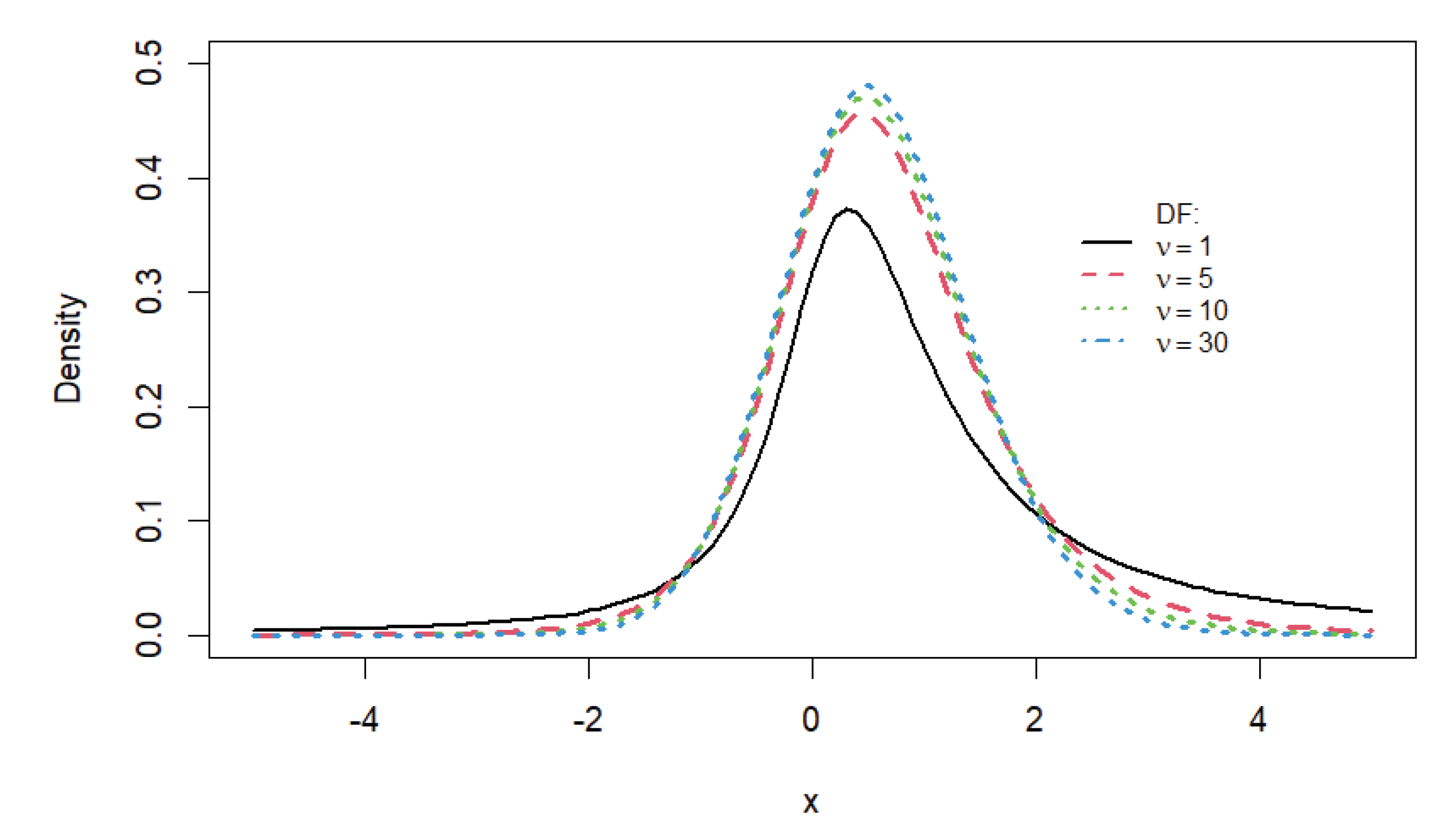
Figure 2.
Critical values for various parameter values. at sample size at levels of significance
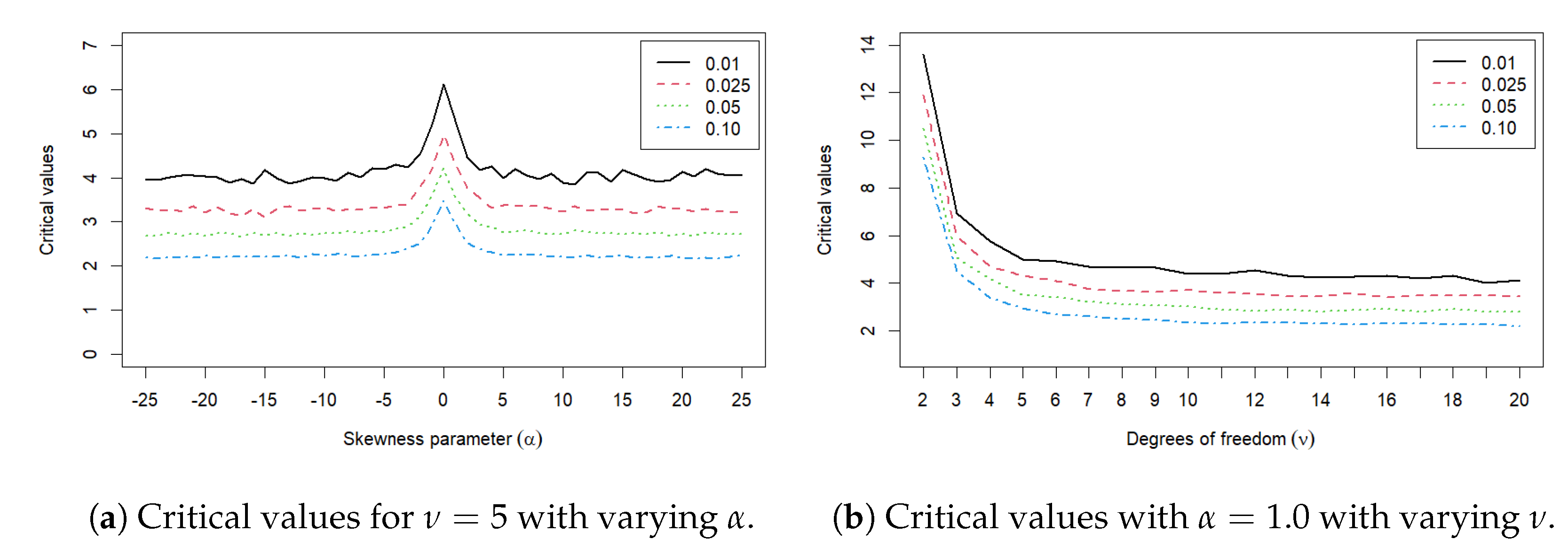
Figure 3.
Histogram, density curves, and CDFs of The body mass index (BMI) of 102 male Australian Athletes.
Figure 3.
Histogram, density curves, and CDFs of The body mass index (BMI) of 102 male Australian Athletes.
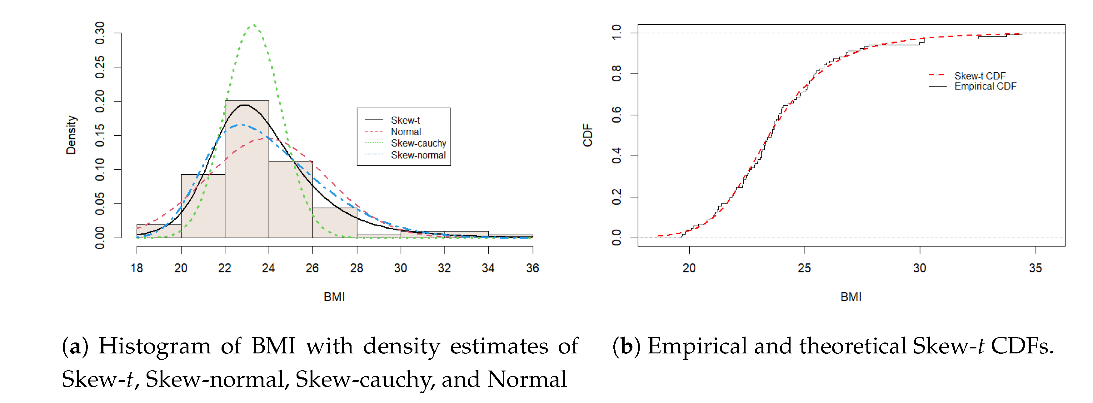
Figure 4.
Histogram, density curves, and CDFs of Apple’s daily returns with 248 observations.
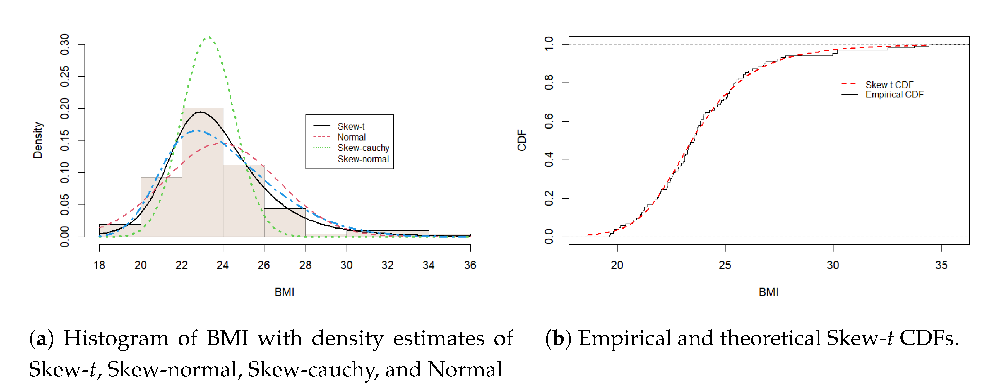
Table 1.
Simulated Critical Values for Energy Statistic of Skew- Distribution
| n | (1,5) | (0,5) | (-1,5) | (1,10) | (0,10) | (-1,10) | (1,30) | (0,30) | (-1,30) | |
| 50 | 3.7856 | 3.8663 | 4.0781 | 2.0441 | 1.9596 | 1.9143 | 1.3624 | 1.3332 | 1.3421 | |
| 100 | 4.5742 | 4.6635 | 4.6401 | 2.3416 | 2.3314 | 2.3443 | 1.6584 | 1.5815 | 1.6448 | |
| 150 | 5.3913 | 5.6910 | 5.3485 | 2.8291 | 2.8642 | 2.8279 | 2.0239 | 2.0291 | 2.0270 | |
| 200 | 6.3893 | 6.6986 | 6.3946 | 3.3414 | 3.4878 | 3.3710 | 2.4003 | 2.4172 | 2.3981 | |
Table 2.
Simulated size of the test for Skew- Distribution
| n | (1,5) | (0,5) | (-1,5) | (1,10) | (0,10) | (-1,10) | (1,30) | (0,30) | (-1,30) | |
| 50 | 0.0508 | 0.0532 | 0.0513 | 0.0476 | 0.0508 | 0.0513 | 0.0510 | 0.0484 | 0.0540 | |
| 100 | 0.0484 | 0.0476 | 0.0492 | 0.0511 | 0.0487 | 0.0503 | 0.0501 | 0.0558 | 0.0488 | |
| 150 | 0.0496 | 0.0506 | 0.0524 | 0.0513 | 0.0509 | 0.0491 | 0.0478 | 0.0492 | 0.0508 | |
| 200 | 0.0503 | 0.0494 | 0.0506 | 0.0505 | 0.0498 | 0.0501 | 0.0497 | 0.0496 | 0.0499 | |
Table 3.
Power Comparison with
| Distribution | Sample size n | ||||||
|---|---|---|---|---|---|---|---|
| 50 | 0.8369 | 0.2248 | 0.2134 | 0.2809 | 0.2460 | 0.3878 | |
| 100 | 0.8933 | 0.2924 | 0.2832 | 0.3850 | 0.3298 | 0.5061 | |
| 150 | 0.9559 | 0.4018 | 0.3638 | 0.5103 | 0.4288 | 0.6223 | |
| 200 | 0.9715 | 0.4973 | 0.4418 | 0.6184 | 0.5069 | 0.7270 | |
| 50 | 0.1066 | 0.0342 | 0.0396 | 0.0332 | 0.0382 | 0.0372 | |
| 100 | 0.1736 | 0.0356 | 0.0418 | 0.0392 | 0.0380 | 0.0384 | |
| 150 | 0.2268 | 0.0360 | 0.0398 | 0.0334 | 0.0382 | 0.0378 | |
| 200 | 0.2790 | 0.0387 | 0.0410 | 0.0413 | 0.0393 | 0.0397 | |
| 50 | 0.8413 | 0.2640 | 0.2491 | 0.3069 | 0.2692 | 0.4092 | |
| 100 | 0.9152 | 0.5090 | 0.4924 | 0.5538 | 0.5140 | 0.6128 | |
| 150 | 0.9655 | 0.6496 | 0.6224 | 0.7012 | 0.6486 | 0.7702 | |
| 200 | 0.9848 | 0.7439 | 0.7169 | 0.8012 | 0.7421 | 0.8601 | |
| 50 | 0.5734 | 0.1145 | 0.1292 | 0.1345 | 0.1302 | 0.1545 | |
| 100 | 0.6045 | 0.2131 | 0.2154 | 0.2546 | 0.2328 | 0.261 | |
| 150 | 0.6401 | 0.3032 | 0.3072 | 0.3844 | 0.3498 | 0.3958 | |
| 200 | 0.6749 | 0.4166 | 0.4196 | 0.5184 | 0.4742 | 0.5261 | |
| 50 | 0.9596 | 0.1128 | 0.1166 | 0.1306 | 0.1188 | 0.3350 | |
| 100 | 0.9916 | 0.1562 | 0.1860 | 0.2004 | 0.1966 | 0.4480 | |
| 150 | 1.0000 | 0.2306 | 0.2756 | 0.3228 | 0.3232 | 0.5816 | |
| 200 | 1.0000 | 0.3030 | 0.3798 | 0.4278 | 0.4292 | 0.6720 | |
| 50 | 0.9701 | 0.3331 | 0.1950 | 0.3988 | 0.2304 | 0.4611 | |
| 100 | 0.9931 | 0.33691 | 0.2092 | 0.3974 | 0.2441 | 0.4644 | |
| 150 | 0.9995 | 0.3449 | 0.2179 | 0.4102 | 0.2586 | 0.4775 | |
| 200 | 0.9998 | 0.3639 | 0.2409 | 0.4429 | 0.2818 | 0.5155 |
Table 4.
MLE, LogL, AIC and SIC values for BMI dataset
| Skew-t | Normal | Skew-cauchy | Skew-normal | |
|---|---|---|---|---|
| 21.6490 | 23.9036 | 22.7889 | 20.8765 | |
| 2.6570 | 2.7403 | 1.3762 | 4.0610 | |
| 1.6421 | - | 0.5126 | 3.2992 | |
| 4.5503 | - | - | - | |
| LogL | -236.0511 | -248.0613 | -247.5519 | -237.9670 |
| AIC | 480.1022 | 500.1227 | 501.1037 | 481.9341 |
| SIC | 490.6020 | 505.3726 | 508.9787 | 489.8090 |
Table 5.
MLE, LogL, AIC and SIC values for Apple stock daily return dataset
| Skew-t | Normal | Skew-cauchy | Skew-normal | |
|---|---|---|---|---|
| 0.5254 | 0.2749 | 0.1798 | 1.3519 | |
| 1.1514 | 1.4259 | 0.7655 | 1.7858 | |
| -0.2285 | - | 0.1191 | -1.1688 | |
| 5.3556 | - | - | - | |
| LogL | -431.3161 | -440.3975 | -461.9316 | -438.1367 |
| AIC | 870.6321 | 884.795 | 929.8633 | 882.2733 |
| SIC | 884.6858 | 891.8219 | 940.4036 | 892.8136 |
Table 6.
Summary of test statistics and corresponding p-values of BMI data
| Test | ||||||
|---|---|---|---|---|---|---|
| Statistic value | 1.7109 | 0.0454 | 0.8731 | 0.0295 | 0.0290 | 0.2321 |
| P-value | 0.5840 | 0.9847 | 0.9847 | 0.9827 | 0.9840 | 0.9807 |
Table 7.
Summary of test statistics and p-values of Apple daily return data
| Test | ||||||
|---|---|---|---|---|---|---|
| Statistic value | 3.9635 | 0.0357 | 1.0576 | 0.0291 | 0.0290 | 0.1737 |
| P-value | 0.5473 | 0.8260 | 0.8167 | 0.9381 | 0.9380 | 0.9913 |
Disclaimer/Publisher’s Note: The statements, opinions and data contained in all publications are solely those of the individual author(s) and contributor(s) and not of MDPI and/or the editor(s). MDPI and/or the editor(s) disclaim responsibility for any injury to people or property resulting from any ideas, methods, instructions or products referred to in the content. |
© 2025 by the authors. Licensee MDPI, Basel, Switzerland. This article is an open access article distributed under the terms and conditions of the Creative Commons Attribution (CC BY) license (http://creativecommons.org/licenses/by/4.0/).
Copyright: This open access article is published under a Creative Commons CC BY 4.0 license, which permit the free download, distribution, and reuse, provided that the author and preprint are cited in any reuse.


