
Submitted:
23 September 2025
Posted:
24 September 2025
You are already at the latest version
Abstract
The article considers the description of a macrosystem in terms that do not depend on the nature of the macrosystem. The results obtained can be used to describe macrosystem models of thermodynamic processes, and to create interdisciplinary models that take into account interactions of various nature. The macrosystem model is based on its representation in the form of a self-similar coloured oriented multigraph, for each node of which the equation of state is fulfilled, which connects extensive variables. One of the extensive variables is entropy, the maximum of which corresponds to the state of equilibrium. For processes in which fluxes are linearly dependent on driving forces, Onsager's relations are shown to be true, which makes it possible to prove that in the space of stationary processes, entropy production in a closed macrosystem is a metric similar to the Mahalanobis metric, which determines the distance between processes. Zero in such a space are reversible processes, thus the production of entropy shows the degree of irreversibility, as the distance from a researched process to a reversible one.
Keywords:
thermodynamic processes
; macrosystem
; entropy production
; extensive variables
; intensive variables
; measure space
1. Introduction
Thermodynamics has historically been the first and main research field of the complex systems [1]. It is thermodynamic analogies that are used in the description of other systems such as economic, social, informational, algorithmic ones, when control is only possible in an averaged sense. We mean averaged because it is impossible to observe or control the state and behaviour of individual elementary particles, whose large aggregate forms a complex system.
In a thermodynamic system, the elementary particles are molecules. The reason of phenomenological (i. e., experimentally observable) patterns related to the state of a thermodynamic system is carried out through dynamic or statistical averaging of the interactions between individual molecules. However, such averaging is only possible under a priori assumptions about the nature of such interactions as they cannot be verified due to the incredibly large number of molecules in the system and their extremely small size, which makes them neither observable nor controllable [2].
The validity of such a framework is supported by the existence of phenomenological laws. However, in this case, the assumptions about the properties of individual molecular interactions must be derived from the observations of thermodynamic systems as they cannot serve as proof of the truth of the phenomenological laws per se.
The approach suggested in this work is the reverse one, based on a structural induction, where the basic point is any scale level at which the properties of the system can be experimentally verified. This presupposes the fulfilment of the self-similarity condition, which is generally defined as follows: A set X is self-similar if there exists a finite set K indexing a collection of injective and non-surjective mappings , such that [3]. The self-similarity condition is actively used in thermodynamics [4], even though it is strictly fulfilled only when the set of subsystems whose union forms the given thermodynamic system is a continuum. This assumption is too strong for real thermodynamic systems but can be considered a good approximation.
The approach considered below is not limited to describing thermodynamic systems alone, but is intentionally extended to a more general representation. This allows for the consideration of a class of macrosystem models that includes thermodynamic systems.
2. Definition of Macrosystems
When analysing patterns that arise in the exchange processes in systems of various nature: physical, chemical, economic, informational, and social, it is often advisable to use a macrosystem approach.
Macrosystems are systems for which the following conditions are satisfied:
- Macrosystems consist of a large number of elementary objects, and this number is so large that any macrosystem can be considered as a continuum and can be divided into any finite number of subsystems, including those sufficient to determine the statistical characteristics of any given accuracy; each of the subsystem can be considered as a macrosystem. Any macrosystem is a nonempty collection of subsets of closed under complement, countable unions, and countable intersections. is a σ-algebra and ordered pair is a measurable space. The macrosystem can be considered as a union of a finite number of a lower level macrosystems : . This condition is called the self-similarity condition [5].
- The macrosystem state is determined by the vector of state variables. They are assumed to satisfy the conservation law; therefore, we can consider them as a vector of extensive variables. Because of non-negativity and countable additivity, vector is a vector measure and is a measure space. In thermodynamic macrosystems extensive variables are internal energy, mass, and volume [6], which the macrosystem can exchange with its external environment [7]; we will also consider the external environment as a set of macrosystems (and a higher level macrosystem is the union of the macrosystem and its external environment). In the process of interaction between the subsystems X and Y, the values of the vectors and change over time. In this way, exchange processes and their corresponding fluxes are formed, understood as the rates of change of the extensive quantities. We will denote fluxes between subsystems and as .
-
It is impossible to control each elementary object due to their extremely large number [7]. The macrosystem control can be organized only by impact on the parameters averaged over a set of elementary objects, namely:
- -
- change in the parameters of the macrosystem’s external environment, the interaction with which determines the change in the stock of extensive variables in the macrosystem;
- -
- change in the stock of extensive variables (for example, their extraction) in the macrosystem due to external interventions;
- -
- changing the characteristics of the exchange infrastructure to accelerate or, conversely, slow down the exchange processes.
3. Representation of the Macrosystem as a Multigraph
The macrosystem can be represented as a self-similar oriented weighted multigraph, the nodes of which correspond to the subsystems and the macrosystem’s external environment, and the edges correspond to the fluxes between the subsystems and between the subsystems and the macrosystem’s external environment. Each graph node (each subsystem) is characterized by a vector , and fluxes between subsystems can be functionally unrelated to each other.
Self-similar – each graph node can be represented as a graph that describes the interaction of subsystems that form this node with each other and with their environment. Let us consider two interacting (vector of fluxes of extensive variables is ) macrosystems and . Due to self-similarity condition we can introduce sets corresponding to these macrosystems. Each subsystem is characterized by its own stock: for and for . Flux is formed between subsystems from different sets and . In this notation, following equations are valid:
Oriented – the direction of each edge determines the positive sign of each flux; thus, if the edges are directed from node to node , then:
However, edges of different colours corresponding to different extensive variables can be either co-directed or opposite.
Weighted – the weight of the edge shows the flux intensity: the positive value of the -th flux , if the real flux of the extensive variable is directed towards the edge, , if it is opposite to the edge’s direction. In addition, a matrix of infrastructure coefficients is determined for all fluxes between nodes and (that is, for all fluxes ). This matrix is the metadata for the edges connecting nodes and , and determines both facility of exchange process and complementary or substitutionary features of the extensive variables [8].
Multigraph – two graph nodes can be connected both by edges of different colours, and by groups of edges of different colours, which corresponds to multiple contact points between subsystems. The absence of edges between the multigraph’s nodes means that the nodes are isolated from each other.
Figure 1 shows an example of the self-similar oriented weighted multigraph of a part of a macrosystem.
4. Equilibrium State of the Macrosystem
Let us assume that two macrosystems and exchange the vector of the extensive variables . At each moment of time t, the reserves of the extensive variables describing the state of macrosystems are equal to . We represent macrosystems as a union of a finite set of subsystems: , respectively. An equilibrium state shall be a state in which the sum of fluxes at each moment of time for each
Thus, the equilibrium in the macrosystem is considered as dynamic. The equilibrium condition can be defined as follows: at the any level of sets of subsystems vector of fluxes is described by a time-independent distribution with expectation .
Note that the fluxes , , and the random variable , which describes the subsystem fluxes distribution, are vectors. At this level of subsystems, we can assume a large number of factors affecting the distribution of fluxes, which means that the distribution can be described by a multivariate normal distribution. The parameters of this distribution are the expectation , which determines fluxes at the level of subsystems and in accordance with (3), and the covariance matrix .
Assuming that fluxes arise due to the activity of some driving forces, which we can also consider at the subsystem level as a random vector, such that:
- -
- fluxes are linearly dependent on the exchange driving forces [6]: – under this assumption and suggesting that the matrix of infrastructure coefficients is constant, the driving forces distribution is also normal;
- -
- the covariance matrix of subsystems of the macrosystem depends on the driving forces intensity , causing these fluxes, so that the matrices and are jointly normalizable (their eigenvectors coincide) – due to the linear relationship between fluxes and driving forces;
- -
- limits of correlation coefficients corresponding to the covariance matrix for any : due to the redistribution of the extensive variables over a variety of subsystems, depending on the number of intermediate nodes of a given colour in the multigraph chain to the contact point.
If the equilibrium condition is satisfied for a macrosystem when interacting with each macrosystem from its environment, then such a macrosystem is called closed. If for a macrosystem all its subsystems are in equilibrium when interacting with each other (but not necessarily with the environment of the macrosystem ):
then we call this macrosystem to be in a state of internal equilibrium. For a macrosystem in internally equilibrium, all fluxes can be observed only at the boundaries of the macrosystem and its environment.
5. Extensive and Intensive Variables
Let us assume that two macrosystems and exchange the vector of the extensive variables . At each moment of time , the stocks of the extensive variables describing the state of macrosystems.
The macrosystem shall be described by a set of extensive and intensive variables:
- -
- extensive variables are such that for any two macrosystems and (not necessarily in equilibrium)due to conservation law all the stocks of the extensive variables are extensive variables;
- -
- intensive variables are such that for any two systems X and Y that are in equilibrium,
Extensive variables satisfy the neutral scale effect condition: if all extensive variables in all subsystems of the macrosystem are increased by times, then the fluxes intensities in the macrosystem will not change. In particular, such a proportional increase in the extensive variables will not bring the macrosystem out of the internal equilibrium state, if before that the system was in internal equilibrium. The proof of this assertion is given in Section 6.
As a consequence of (6) intensive variables dependences on the extensive variables stock that determine the macrosystem state, should be homogeneous functions of the zero-order.
6. Entropy of the Macrosystem
The set of extensive variables describes the macrosystem state. Among the extensive variables we single out the value , which characterizes the objective function of the system. and other extensive variables are functionally related: , . We call this equation the system state equation.
The choice of S as the objective function is determined by the Levitin–Popkov Axioms [9], which impose the following conditions on this variable:
- For a controlled system, given a fixed deterministic control , its stochastic state which is characterized by a vector flux is transformed into a deterministic vector , called the steady or stationary state, which belongs to the admissible set .
-
For any fixed vector , there exists a vector of a priori probabilities for the distribution of fluxes in the system , such that the stationary state of the macrosystem under the given fixed control is the optimal solution to the entropy-based optimization problem: , where is the entropy operator defined asThus, the pair simultaneously provides both the required vector of prior probabilities and the corresponding stationary state vector.
- There exists a inverse mapping such that the desired pair is the unique solution to the system of the relations:
Within the framework of the considered model, these statements can be interpreted as follows:
- For any fixed deterministic control , there exists a stable steady state .
- The stable steady state is a state of an internal equilibrium corresponding to the maximum of .
- The stable steady state is unique.
For a closed system, the condition , determines the spontaneous direction of exchange of extensive variables. However, a question arises about the homogeneity of the function : entropy is a homogeneous function of degree one only in the systems that are in a state of internal equilibrium. In cases where the distribution is scale-invariant but does not correspond to internal equilibrium, a fractal structure of the macrosystem is observed, in which is a homogeneous function with a degree of homogeneity less than one. Taking this remark into account, entropy can still be considered an extensive quantity. The question to use the degree of homogeneity as a measure of equilibrium of the macrosystem should be given further consideration.
Since is an extensive variable in the condition of internal equilibrium, then is a homogeneous function of the first-order: when scaling the system by times or combining identical macrosystems in the equilibrium state:
In accordance with the Euler relations for homogeneous functions
Let us denote . Since is a homogeneous function of the first-order, then are homogeneous of the zero-order, i. e. they are intensive variables: for any value . This means that a proportional increase in the extensive variables will not bring the macrosystem out of the internal equilibrium state, if before that the system was in internal equilibrium.
Under the assumption that the function is differentiable and its partial derivatives are continuous, in accordance with the necessary condition for the function to be differentiable, there exists a total differential
Two consequences of equation (11) can be formulated:
Consequence 1. By differentiating the Euler relation (10) we obtain:
By comparing (11) and (12) we see that the second term in (12) should be equal to zero:
Consequence 2. The exchange process between subsystems and (with a positive direction of fluxes from to ) can be described using equations (2) and (11) as follows:
The parameter is extensive variable and its dependence on other state variables is objective function for spontaneous processes in the macrosystem.
From the established relations, the following conclusion can be drawn:
Let Q be a vector measure on a measurable space .. Then, the entropy of a subsystem is defined as a function , such that:
- -
- , where is the entropy of X under internal equilibrium of all subsystems X;
- -
- , where is the entropy of a subsystem with a zero-vector measure;
- -
- For any two subsystems such that , , it holds that .
These properties correspond to Shannon – Khinchin Axioms for entropy [10]. So statistically corresponds to the entropy of the distribution of state parameters of subsystems of the macrosystem. Let us explain this statement. Since there are no restrictions on the possible random vector values with a finite variance, the normal distribution corresponds to the maximum entropy value (this can be considered as a justification for the distribution law of subsystems parameters that form a macrosystem).
The entropy of the normal distribution consists of two terms: , where is the correlation matrix, the first addend corresponds to the complete independence of the system elements and characterizes the structure of the macrosystem, and the second describes the relationships in the macrosystem. As the correlation between fluxes increases, which is observed with the growing magnitude of the exchange driving forces . Figure 2 illustrates the kind of dependency of . The second term of entropy expression, always negative at , ( is the identity matrix), decreases. This explains the statement about as an objective function that reaches its maximum when the macrosystem reaches an equilibrium state, and a state function that sets the direction of processes in a closed system, increasing the dispersion of low-level subsystem parameters while simplifying the macrosystem structure at a high level.
In the process of spontaneous, not forced exchange, the value of a closed macrosystem cannot decrease, since is the objective function for the system behaviour. In order for the value , called the entropy production, to be positive during the any process of given non-zero intensity, it is sufficient to fulfill the condition
If the process duration is infinitely long, then the macrosystem’s natural evolution leads it to a state of internal equilibrium, which corresponds to the achievement of the maximum value. This is equivalent to the statement that in the internal equilibrium state is maximum.
Intensive variables can be considered as specific potentials. Their difference according to (15) is the driving force of the exchange process. The fluxes are directed from subsystems with lower values of intensive parameters to subsystems with higher values of intensive parameters. Thus, equation (14) can be rewritten as follows:
where is the matrix of infrastructure coefficients. Note that infrastructure of the exchange process involves wide variety of features of the subsystems’ boundaries medium. For example, in thermodynamic macrosystems these features are surface area, roughness, etc. All these parameters can be controls in the corresponding optimization problems, but here is assumed to be constant. If the driving force during the process is constant, then such a process is called stationary. Among the stationary processes, we single out the classes of reversible () processes and processes of minimal dissipation .
7. Differential Form of the State Equation
The state function can be given in differential form as is typical for thermodynamic systems:
This is thermodynamic point of view: there is no state function described in the terms of extensive variables. This poses the question about the integrability of the function . Equation (17) is the Pfaffian form. A Pfaffian form is said to be holonomic if there exists an integrating multiplier such that
The Pfaffian form of two independent variables is always holonomic, that is, there is always an integrating multiplier . However, for , the integrating multiplier exists if the holonomy conditions are satisfied: for any three different
These conditions are obtained from the equality of the second mixed derivatives with respect to any variable pairs (Maxwell’s relations)
and by exclusion of the integrating factor from these equalities. In addition to conditions (19), it is necessary that all products be homogeneous of zero-order homogeneity.
8. Concavity of Entropy Function
The function gradient determines the intensive variables vector of the macrosystem. As the extensive variables increases, the value also increases, but at a slower rate (the diminishing returns law), so that for all . Moreover, the Hessian matrix for homogeneous functions of the first-order homogeneity is negative semi-definite. Indeed, it follows from the Euler relations (10): differentiating both parts of this equation per it turns out that
For an arbitrary vector , the necessary conditions for the extremum of a quadratic form in
which corresponds to the maximum point (according to the diminishing returns law) of the quadratic form . Since the product (21) is equal to zero, then at the maximum point is also equal to zero. Thus, for any value of , which was to be proved. Note that since the Hesse matrix is symmetric, then all its eigenvalues are real numbers.
The negative semi-definiteness of the Hessian matrix corresponds to the upward convexity (concavity) of function and unimodality as the objective parameter. As the reserves of the extensive variables in the macrosystem increase, increases, and the intensive parameters decrease, reducing the magnitude of the resource exchange driving force. In accordance with (14), this behaviour of intensive parameters leads to the fact that when the macrosystem is affected, changing its internal equilibrium conditions, the resource exchange processes are directed towards counteracting changes, thus the Le Chatelier principle is fulfilled.
Partial derivatives describe the saturation of the system with the extensive variables, and determine the substitution and complementation of the extensive variables in the macrosystem. If the extensive variables are substitutes, then an increase in one of them reduces the intensive variables adjoined with the other extensive variable. If the extensive variables are complements, then an increase in one of them, on the contrary, increases the intensive variables adjoined with the other extensive variable.
9. Metric Features of Entropy
Let us consider a particular case of exchange processes in a macrosystem consisting of two subsystems and , where the fluxes linearly depend on the differences between the intensive variables of the subsystems:
where .
Proposition
Matrix is the matrix of infrastructure coefficients describing the exchange possibilities at the boundary between subsystems, and it is a symmetric matrix.
Proof.
Given the self-similarity property, the system can be divided into a statistically significant disjoint set of subsystems such that the characteristics of these subsystems form a representative sample of random variables , etc. The eigenvectors of the matrices and coincide and form a system of orthonormal vectors. Since the eigenvectors of any matrix and its inverse are the same, and are symmetric and commutative, so their product is a symmetric matrix. Since , the matrix of phenomenological coefficients is symmetric (Onsager conditions).
Proposition.
Matrix is a positive definite matrix.
Proof.
The right part of equation (16) under condition (24) is a quadratic form
For any positive values of the exchange driving forces , the entropy production is positive. Therefore, is a positive definite matrix. It means that of the dependencies and under the linear dependence of the flows on the driving forces are convex.
The consequence of this proposition is entropy production is a metric in the space of stationary processes and can be used to determine the distance between processes
Let us present some properties of this metric:
- -
- zero in the space of stationary processes is reversible processes for which . According to the third Levitin – Popkov axiom there is the only reversible process in the macrosystem;
- -
- the distance between two processes and is determined as . It is evident that ;
- -
- the distance satisfies the triangle inequality due to is a positive definite symmetric matrix, all its eigenvalues are positive real numbers.
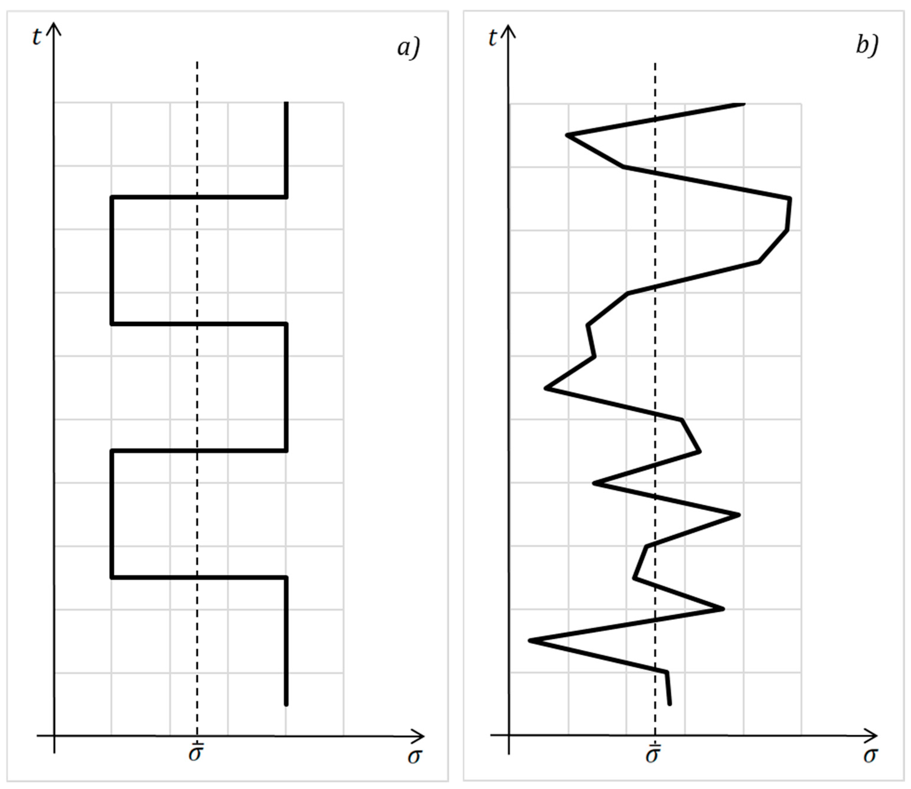
Thus, the entropy production in a macrosystem characterizes the distance of stationary exchange processes occurring in such a system from the corresponding reversible process. For linear systems it is possible to consider generalized, averaged over probability measure stationary process: . For cyclic and stochastic processes such an averaging is illustrated on Figure 3.
10. Trajectories of the Exchange Process
For non-stationary exchange processes, it is necessary to determine the trajectory of the process: the change in time of all subsystems parameters when approaching the equilibrium state. For a linear dependence between fluxes and driving forces (24), we derive a differential equation that determines the change in the driving forces of the exchange process in a macrosystem consisting of two subsystems and . Under given initial conditions , this equation describes all the parameters of the subsystems.
Full differentials of functions shall be written as:
Subtracting the equations for subsystem from the equations for subsystem , taking into account the linear dependencies of fluxes on driving forces (24) and the fact that the driving forces are the differences between the corresponding intensive variables of the subsystems: , we obtain
Equation (28), together with the initial conditions, determines the trajectory of the exchange process.
5. Conclusions
The metric properties of entropy production allow to determine both the class of minimally irreversible processes [11] and the quantitative distance between the processes. The stationarity restriction can be removed by averaging process parameters over time. A generalized, independent of the nature of the processes, macrosystem model is useful for formalization and investigation of extreme performance of complex, hierarchically related systems. In these macrosystem there is a vector of entropy functions and the distance between the processes is a vector too. It gives the macrosystem additional degree of freedom at the level of subsystems.
The given proofs of the phenomenological properties of macrosystems are valid for thermodynamic systems but can also be applied to the systems of a different nature, particularly economic systems [12,13], information exchange systems in communication networks [14], and high-performance computers [15], where the number of computational cores is already comparable to the number of molecules in 1 μm³ of gas. The main difference in the description of macrosystems of different natures lies in the definition of the extensive quantities that describe the state of a system and in the relationships between the fluxes that arise from interactions between subsystems. In thermodynamic macrosystems extensive variables are internal energy, mass, and volume [6], in economic macrosystems extensive variables are resources, goods and welfare [12], in information macrosystems like recommendation systems extensive variables are database size and the number of exposed marks [16], and so on. In information macrosystems we restrict ourselves to describe syntactic information exchange [17]. Social macrosystems with semantic and pragmatic information exchange processes require a special conceptual apparatus, markedly different from the one usually used in formal logic [18].
For signal transmission systems, the extensive variables are the number of processors of a given type, the amount of memory; the entropy properties of the computing power; and the intensive variables are determined by the contribution to the increase in computing power that each type of hardware provides. When modelling algorithms as complex systems, the extensive variables can be used as control values, the entropy corresponds to the objective function, and the intensive variables are the values of the Lagrange multipliers. Economic analogies of complex systems are often considered. At the micro level, extensive quantities include the stock of goods, while intensive quantities include the prices and the values of the goods. The welfare function has the properties of entropy in microeconomic systems. At the macro level, it is advisable to choose the gross regional product as the entropy, as a function of vector of production factors. The intensive variables in this model are prices in real terms.
The specific behaviour of individual elementary entities which is especially relevant for social systems, where free and often unmotivated decision-making is possible can complicate the application of the model. Nevertheless, the model can still be used to describe processes of various natures occurring simultaneously within a system. For example, a high-performance computer can be represented in this way as a macrosystem in which hardware, software, and engineering subsystems exchange energy, signals, and information, and the average intensities of the computational processes and heat transfer processes are considered to be given. Any computer does not perform mechanical work; therefore, all consumed electrical energy is converted into heat and must be dissipated into the surrounding environment.
Acknowledgments
The author have reviewed and edited the output and take full responsibility for the content of this publication. This research received no funding.
References
- Andresen, B.; Salamon, P. Future Perspectives of Finite-Time Thermodynamics. Entropy 2022, 24, 690. [CrossRef]
- Fitzpatrick, R. Thermodynamics and Statistical Mechanics. World Scientific Publishing Company, 2020, 360 p. ISBN: 978-981-12-2335-8.
- Prunescu, M. Self-Similar Carpets over Finite Fields. European Journal of Combinatorics 2009, vol. 30 (4), p. 866 – 878. [CrossRef]
- Tropea, C.; Yarin, A. L.; Foss, J. F. Springer Handbook of Experimental Fluid Mechanics. Springer-Verlag, 2007, 557 p. ISBN: 978-3-54-030299-5.
- Popkov, Yu. S. Macrosystem Models of Fluxes in Communication-Computing Networks (GRID Technology). IFAC Proceeding Volumes 2004, vol. 37 (19), pp. 47 – 57. [CrossRef]
- Rozonoér, L. I. Resource Exchange and Allocation (a Generalized Thermodynamic Approach). Automation and Remote Control 1973, vol. 34 (6), pp.915 – 927.
- Popkov, Yu. S. Macrosystems Theory and its Applications. Equilibrium Models. Ser.: Lecture Notes in Control and Information Sciences. 203. Springer Verlag: Berlin, 1995. 323 p. ISBN 3-540-19955-1.
- Amelkin, S. A.; Tsirlin, A. M. Optimal Choice of Prices and Fluxes in a Complex Open Industrial System. Open Systems & Information Dynamics 2001, vol. 08 (02), pp. 169-181. [CrossRef]
- Levitin, E. S.; Popkov, Yu. S. Axiomatic Approach to Mathematical Macrosystems Theory with Simultaneous Searching for Aprioristic Probabilities and Stochastic Flows Stationary Values. Proceedings of the Institute for System Analysis RAS 2014, vol. 64 (3), pp. 35 – 40.
- Khinchin, A. I. Mathematical Foundations of Information Theory. Dover, New York, 1957. 120 p. (Original publication in Russian is: Khinchin, A. I. The Concept of Entropy in Probability Theory. Uspekhi Matematicheskikh Nauk 1953, vol. 8, No. 3 (55), p. 3 – 20).
- Tsirlin, A. M. Minimum Dissipation Processes in Irreversible Thermodynamics. Journal of Engineering Physics and Thermophysics 2016, vol. 89 (5), pp. 1067 – 1078. [CrossRef]
- Tsirlin, A. M. External Principles and the Limiting Capacity of Open Thermodynamic and Economic Macrosystems. Automation and Remote Control 2005, vol. 66 (3), pp.449 – 464. [CrossRef]
- Tsirlin, A. M.; Gagarina, L. G. Finite-Time Thermodynamics in Economics. Entropy 2020, vol. 22 (8), 891. [CrossRef]
- Dodds, P.; Watts, D.; Sabel, C. Information Exchange and the Robustness of Organizational Networks. Proceedings of the National Academy of Sciences of the United States of America 2003, 100, 12516-21. https://www.pnas.org/doi/10.1073/pnas.1534702100.
- De Vos, A. Endoreversible Models for the Thermodynamics of Computing. Entropy 2022, 24, 690. [CrossRef]
- Pebesma, E.; Bivand, R. Spatial Data Science: With Applications in R. Chapman and Hall/CRC, Boca Raton, 2023, 314 p. [CrossRef]
- Martinás, K. Entropy and Information. World Futures 1997, vol. 50 (1 – 4), pp. 483 – 493. [CrossRef]
- Jøsang, A. Subjective Logic. A Formalism for Reasoning Under Uncertainty. Springer Cham, 2016, 337 p. ISBN: 978-3-319-42335-7. [CrossRef]
Figure 1.
An example of the self-similar oriented weighted multigraph corresponding to a macrosystem.
Figure 1.
An example of the self-similar oriented weighted multigraph corresponding to a macrosystem.
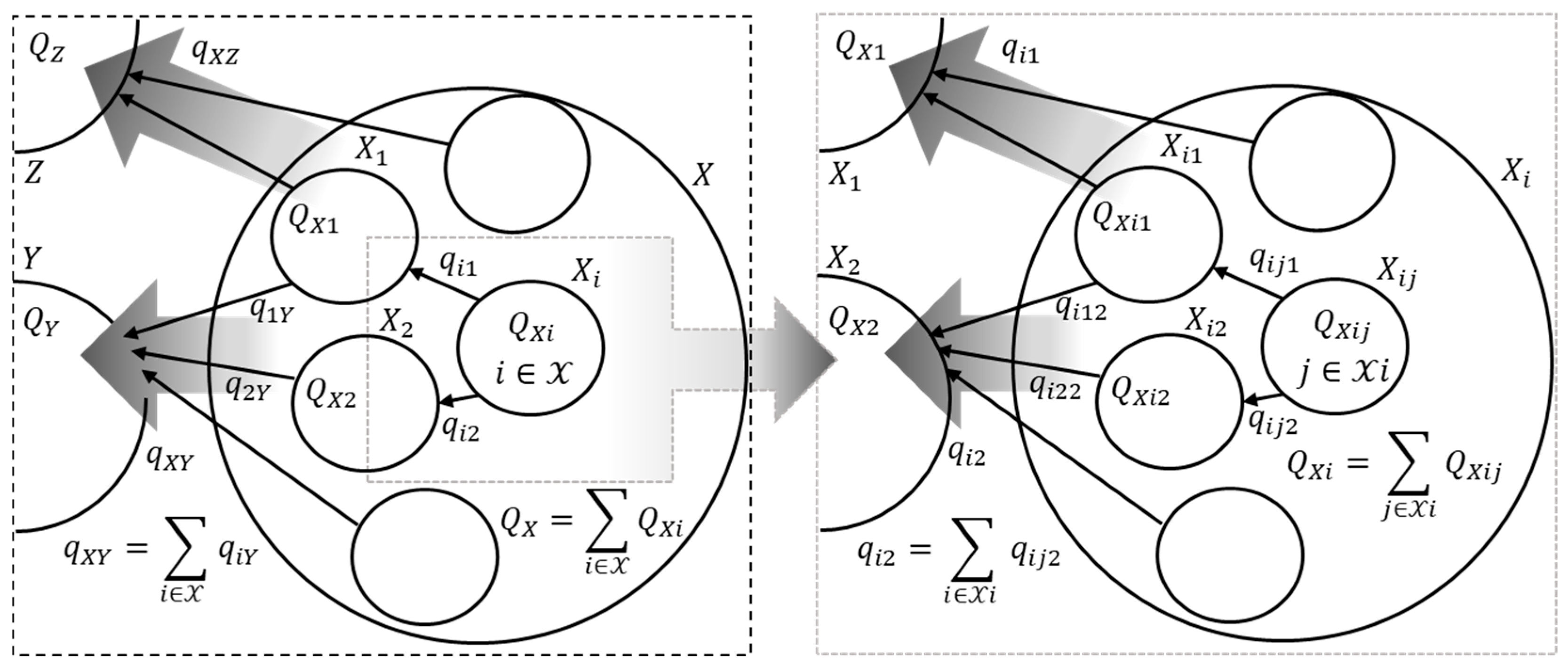
Figure 2.
Dependency of correlation between fluxes in a macrosystem.
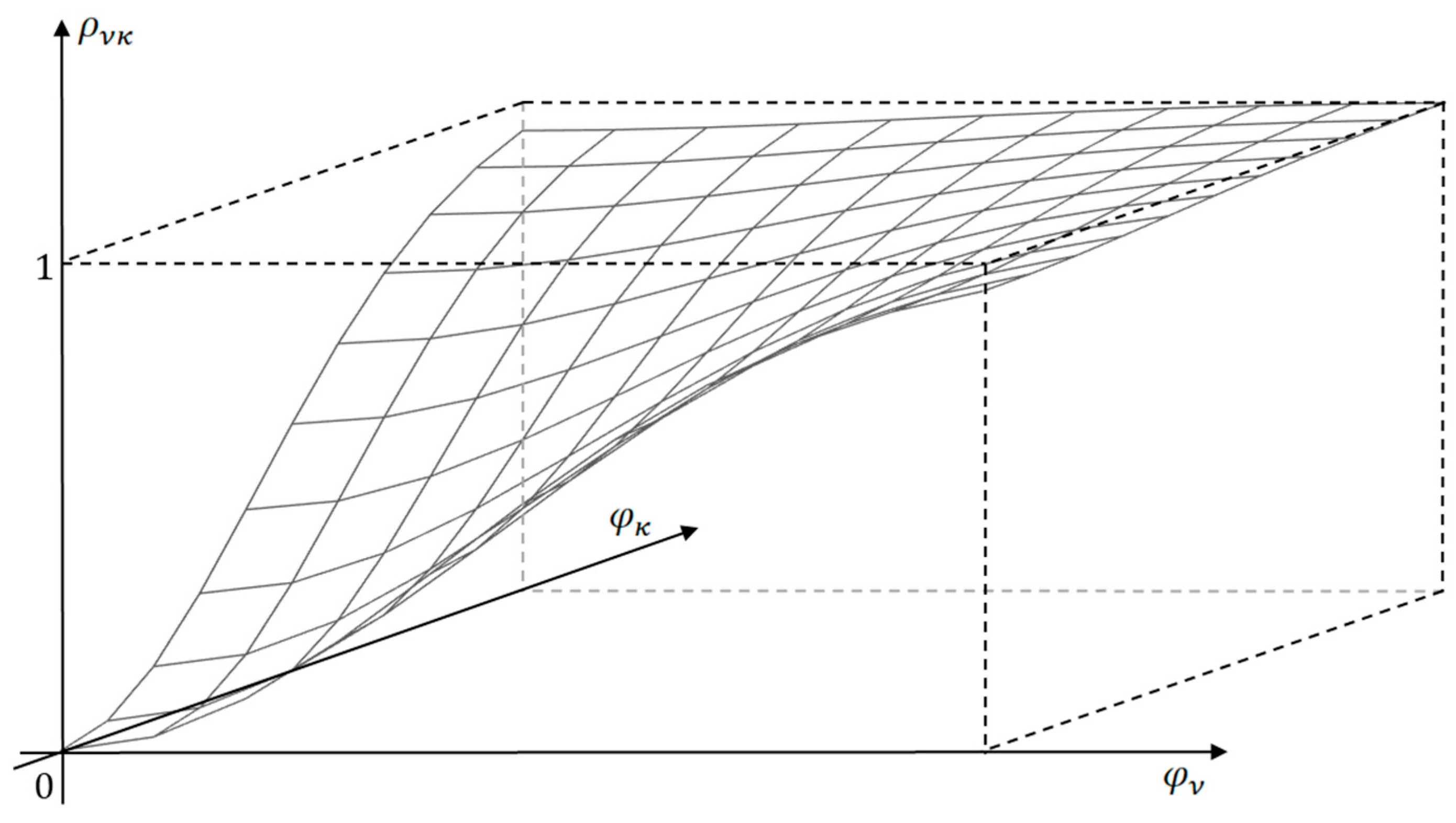
Figure 3.
Averaging of entropy production in cyclic (a), and stochastic (b) stationary processes.
Disclaimer/Publisher’s Note: The statements, opinions and data contained in all publications are solely those of the individual author(s) and contributor(s) and not of MDPI and/or the editor(s). MDPI and/or the editor(s) disclaim responsibility for any injury to people or property resulting from any ideas, methods, instructions or products referred to in the content. |
© 2025 by the authors. Licensee MDPI, Basel, Switzerland. This article is an open access article distributed under the terms and conditions of the Creative Commons Attribution (CC BY) license (http://creativecommons.org/licenses/by/4.0/).
Copyright: This open access article is published under a Creative Commons CC BY 4.0 license, which permit the free download, distribution, and reuse, provided that the author and preprint are cited in any reuse.


