Dynamic Balance: A Thermodynamic Principle for the Emergence of the Golden Ratio in Open Non-Equilibrium Steady States

1. Introduction

The golden ratio, $\phi \approx 1.618$, famously appears in the arrangement of leaves (phyllotaxis), the branching patterns of trees, blood vessels, lightning, and river deltas [1,2,3,4], and the logarithmic spiral arms of galaxies and hurricanes [5,6]. Yet its reach extends far beyond botany and geometry. Recent experiments have uncovered power-law exponents or geometric features related to $\phi$ in a surprising variety of complex systems— rotating turbulence [7,8,9], quantum critical chains [10,11], twisted bilayer graphene (TBG) [12,13,14], Fibonacci anyons [15,16], neural activity exponents [17,18], and more. These complex systems are open, constantly exchanging energy and matter with their environment (solar influx in planetary systems, gravitational potential in rotating systems, biochemical energy in cellular processes), while irreversibly dissipating part of it (thermal conduction, radiative cooling, viscous dissipation, heat in chemical reactions) to maintain their internal structure and optimal functionality. They thrive in this poised non-equilibrium steady-state between rigid order and chaotic disorder.

Classical equilibrium thermodynamics, although extremely powerful, fails to encapsulate many phenomenological aspect of these irreversible processes that we encounter everyday. In particular, the observation of fractals, spirals, branching patterns, and scale-invariant processes in open, driven-dissipative systems operating far-from-equilibrium [19]. The main issue is that the thermodynamic state variables typically used to describe a system (energy, temperature, entropy etc), can all vary widely over time or space in non-equilibrium processes. Therefore, measuring rates of energy input and entropy outflow is often simpler than determining absolute energies.

In this work, we define a dimensionless energy–entropy flux ratio $\alpha \left(t\right)$ that directly quantifies the real-time balance between the energy that goes into useful organization or work relative to the energy irreversibly lost to entropy production. A high $\alpha \left(t\right)$ means the system retains or utilizes a larger portion of its energy (lower relative dissipation), whereas $\alpha \left(t\right)$ close to 1 indicates most energy simply heats the environment with little left to build or maintain structure. Real systems inherently develop negative feedback loops or structural constraints to prevent collapse or complete saturation, thereby stabilizing their internal state. For example, either too high anabolism (structure building) or catabolism (dissipation) can be fatal to biological systems, so they self-regulate through metabolic constrains (hormonal regulation, growth factor inhibition, etc). Therefore, in a sustained non-equilibrium steady-state (NESS), $\alpha \left(t\right)$ will self-adjust to a specific constant value that optimally balances the competing needs for energy utilization vs. dissipation. To find this optimal value, we invoke a self-similarity or scale-invariance argument, requiring the system to reproduce its ratio $\alpha \left(t\right)$ at different scales.

Why Scale Invariance? Because these complex systems we are describing typically have many hierarchical levels—subsystems nested within larger subsystems—and near their critical operating point, they display power-law dynamics and fractal organization. Hence, scale invariance posits that $\alpha \left(t\right)$ remains the same across levels—the whole system’s ratio equals the subsystem’s ratio. Under these assumptions, the stable fixed point is the golden ratio, ${\alpha }^{★}=\phi$, the unique point at which the balance of energy and entropy fluxes is self-consistent across all length and timescales. Any other ratio would not be scale-invariant; for example, if $\alpha \left(t\right)$ were less than $\phi$, then the system is dissipating “too much” relative to structure – the next level down would have a higher ratio, causing $\alpha \left(t\right)$ to increase toward $\phi$. Conversely, if $\alpha \left(t\right)>\phi$, subsystems would dissipate too little (relative to their internal energy) and become prone to instabilities, driving $\alpha \left(t\right)$ down.

In our framework, energy flux space emerges as a distinctly non-equilibrium concept. It represents how energy flows dynamically in open, driven-dissipative systems through a given spatial region or boundary. In equilibrium, fluxes vanish, so this additional dimension collapses. Out-of-equilibrium, it appears to describe how systems move along gradients of energy flux toward a stable non-equilibrium self-dual attractor.

Example 1.

Bathtub Whirlpool Analogy. Imagine a faucet that drips water into a bath at a steady rate ($\dot{E}$) and drains at the bottom, generating entropy ($T\dot{S}$). When the ratio of inflow to outflow stabilizes near a fixed critical value, the water forms a scale-invariant spiraling vortex. This vortex does not arise at maximum or minimum flow ($\alpha \to 0^{+},\infty$), it emerges at a critical point, $\alpha =\phi$, where the system achieves dynamic balance, resulting in a visible, self-similar form. The convex structure of the bathtub keeps the water flow bounded and stable so we will define a scalar potential $R\left(\alpha \right)$ to mirror this convexity.

2. Results

2.1. Defining $\alpha \left(t\right)$

Throughout we consider a driven, open system whose coarse–grained energy and entropy fluxes are once–differentiable functions of time,

$${\dot{E}}_c\left(t\right),T\left(t\right){\dot{S}}_w\left(t\right)\in C^1\left([0,\infty )\right),{\dot{E}}_c\left(t\right),T\left(t\right){\dot{S}}_w\left(t\right)>0.$$

We define the dimensionless energy–entropy flux ratio:

$$\alpha \left(t\right)={\displaystyle \frac{{\dot{E}}_c\left(t\right)}{T\left(t\right){\dot{S}}_w\left(t\right)}}\in (0,\infty ),\alpha \in C^1.$$

(1)

The limits $\alpha \to 0^{+}$ and $\alpha \to \infty$ correspond, respectively, to pure dissipation (entropy dominated) and no entropy outlet (energy dominated), and are therefore forbidden by the second law in any sustained non-equilibrium steady state (see Appendix A).

• Energy Flux ($\dot{E}$): net rate of energy flow into a system (with units of power: Joules per second, or Watts). It quantifies how much external energy is available to maintain structure, perform work, and drive system dynamics.
• Entropy Flux ($T\dot{S}$): power irreversibly lost to the environment (or reservoir) through entropy production that carries heat away. Specifically, $\dot{S}$ is the rate of entropy generation (units of Joules per Kelvin per second), and T is an effective temperature characterizing internal microscopic fluctuations or noise intensity within the system. T is a parameter that shapes the distribution of microstates or the level of random excitations.

We will now show that applying $\gamma$ to (1) and imposing scale invariance gives $\alpha ={\phi }^2/\alpha \Rightarrow {\alpha }^2-\alpha -1=0,$ whose unique positive root is

$${\alpha }^{★}=\phi \simeq 1.618.$$

(2)

2.2. Derivation of $\alpha =\phi$ from Self-Similarity

We introduce a self-similar partition argument where the system fluxes self-organize into a scale-invariance structure:

Lemma 1.

The ratio of total energy to entropy-led dissipation equals the ratio of that dissipation to the leftover (structured) energy $\dot{E}:T\dot{S}:\dot{E}-T\dot{S}$.

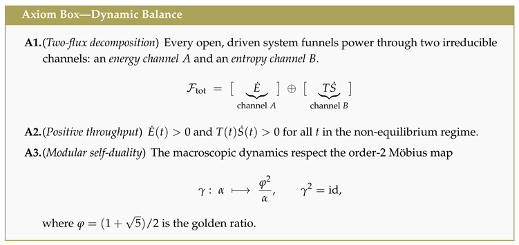
Under Axiom 1, we decompose the system’s energy fluxes into two portions: the energy dissipated in the entropy channel B (${\dot{E}}_B=T\dot{S}$), and the remaining effective work or structure energy ${\dot{E}}_A=\dot{E}-T\dot{S}$. This leftover energy is used to maintain organization, perform work, or is stored in structure. Therefore,

$$\dot{E}={\dot{E}}_A+{\dot{E}}_B=(\dot{E}-T\dot{S})+T\dot{S}.$$

Theorem 1.

Under the assumption of scale-invariant balancing in energy flux vs. heat dissipation across hierarchical levels, the NESS system’s dimensionless ratio must satisfy $\alpha =1/(\alpha -1)$, giving a unique interior attractor ${\alpha }^{★}\equiv \phi$. The key assumption is that the system self-organizes in such a way that the ratio of the total energy to the dissipated part is the same as the ratio of the dissipated energy to the free energy.

Proof. 

Requiring the system to reproduce its balance at different scales means the ratio $\alpha$ for the whole equals the ratio of the part to the remainder:

$$\alpha ={\displaystyle \frac{\dot{E}}{T\dot{S}}}={\displaystyle \frac{T\dot{S}}{\dot{E}-T\dot{S}}}={\displaystyle \frac{1}{\frac{\dot{E}-T\dot{S}}{T\dot{S}}}}={\displaystyle \frac{1}{\frac{\dot{E}}{T\dot{S}}-1}}={\displaystyle \frac{1}{\alpha -1}}.$$

The physically meaningful (positive) solution to the quadratic equation ${\alpha }^2-\alpha -1=0$ is,

$$\alpha ={\displaystyle \frac{1+\sqrt{5}}{2}}=1+{\displaystyle \frac{1}{1+\frac{1}{1+\frac{1}{1+\cdots }}}}=\phi \approx 1.618033...$$

the golden ratio $\phi$, an infinite fraction that captures the essence of self-similarity. This continued nested fraction emerges naturally, explicitly, and uniquely from the modular invariance condition in Axiom 3: $\phi =f\left(\phi \right)=f\left(f\right(\phi \left)\right)$ (see Appendix D). □

2.3. Cost Function $R\left(\alpha \right)$ and Boundary Divergences

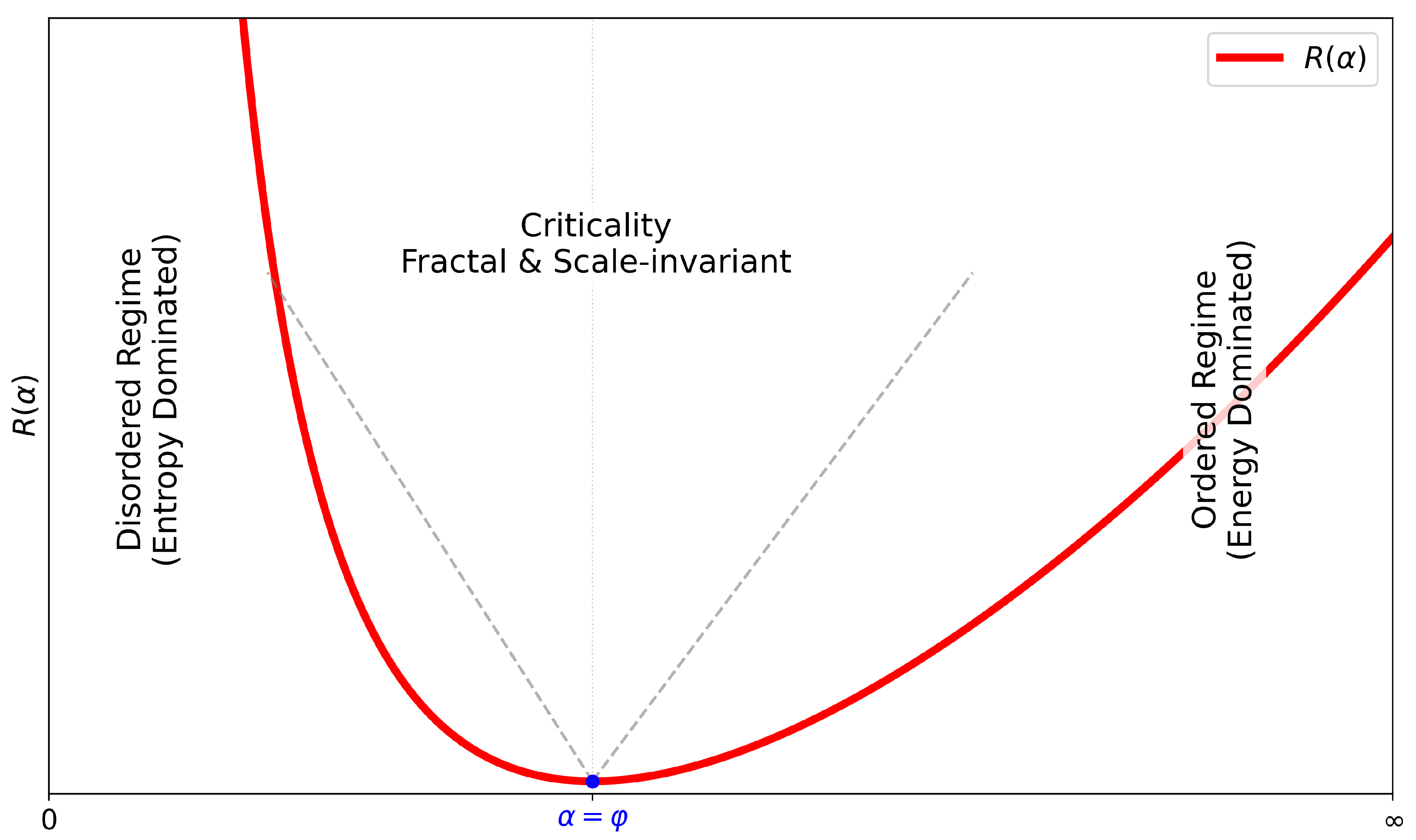
We define a scalar potential or cost function $R\left(\alpha \right)$ to mimic physical thermodynamic constraints and energetic penalties in non-equilibrium conditions. Under the requirements of (i) positivity, (ii) a single interior minimum, and (iii) $\gamma$-invariance, the unique$C^{\infty }$ scalar potential is:

$$R\left(\alpha \right)={\left({\displaystyle \frac{\alpha }{\phi }}-{\displaystyle \frac{\phi }{\alpha }}\right)}^2={\left(x-{\displaystyle \frac{1}{x}}\right)}^2,R\left(\alpha \right)\stackrel{\alpha \to 0^{+},\infty }{\to }\infty ,$$

(3)

which can be expressed in an scale-invariant way by using $x=\alpha /\phi$. We can check that $R\left(\alpha \right)$ vanishes only at ${\alpha }^{★}=\phi \approx 1.618$, and blows up at $0^{+}$ or ∞ (see Figure 1). The golden ratio is the global minimum of the function $R\left(\alpha \right)$ (see Appendix B).

$${\displaystyle \frac{dR\left(\alpha \right)}{d\alpha }}{|}_{\alpha =\phi }=2\left({\displaystyle \frac{\alpha }{\phi }}-{\displaystyle \frac{\phi }{\alpha }}\right)\left({\displaystyle \frac{1}{\phi }}-{\displaystyle \frac{\phi }{{\alpha }^2}}\right)=0,{\displaystyle \frac{d{R}^2\left(\alpha \right)}{d{\alpha }^2}}{|}_{\alpha =\phi }={\displaystyle \frac{8}{{\phi }^2}}\approx 3.055>0.$$

In the bathtub vortex example, no turbulent vortexes form when the water flow is in either extreme, but they spontaneously self-organize at an optimal flow ratio. The shape of the bathtub keeps the water flow bounded and stable, just as our thermodynamic function $R\left(\alpha \right)$, which encodes "hidden" constraints (limited enthalpy, potential energies, or resources) that appear macroscopically as negative feedback. At the stable fixed point ${\alpha }^{★}=\phi$, we have:

$${\displaystyle \frac{T\dot{S}}{\dot{E}}}={\displaystyle \frac{1}{\phi }}\approx 0.618,{\displaystyle \frac{\dot{E}-T\dot{S}}{\dot{E}}}={\displaystyle \frac{1}{{\phi }^2}}\approx 0.382.$$

suggesting that in a system where energy is optimally partitioned between order (free energy) and disorder (thermal entropy), the characteristic balance is given by:

• About 61.8% of energy is thermal entropy ($T\dot{S}$).
• About 38.2% of energy is effective free energy ($\dot{E}-T\dot{S}$).

A compelling body of research on microbial, animal, and plant physiology shows that a fraction ($\sim 60\%--70\%$) of energy inflow is inevitably dissipated as maintenance costs, with the remaining $\sim 30\%--40\%$ channeled into growth, structural buildup, or higher-level functions [20,21,22,23,24,25,26,27].

The ${\mathbb{Z}}_2$ invariance requirement $R\left(\alpha \right)=R({\phi }^2/\alpha )$ under the transformation $\alpha \mapsto {\phi }^2/\alpha$, mean that the global attractor ${\alpha }^{★}=\phi$ represents the unique self-dual point ($\phi$ is a stable, optimal equilibrium point in energy flux space that maps onto itself; see Appendix D). The core transformation is an inversion that flips big to small (order to disorder),

$$\alpha \mapsto {\displaystyle \frac{{\phi }^2}{\alpha }},R\left(\alpha \right)=R\left({\displaystyle \frac{{\phi }^2}{\alpha }}\right),{\dot{E}}_A\leftrightarrow {\dot{E}}_B,$$

(4)

At ${\alpha }^{★}=\phi$, energy and entropy fluxes are optimally balanced, producing stability and scale invariance across multiple scales. Just as the Ising model self-duality (Onsager’s solution), the electromagnetic duality, Kramers-Wannier duality, $S-$ and $T-$ dualities reveal deep universal symmetries in physics, the self-dual point in energy-entropy partitioning points towards universality, optimal efficiency, and emergence of fractals and scale-free structures [28,29].

Theorem 2.

The discrete order-two Möbius flip $\alpha \mapsto \frac{{\phi }^2}{\alpha }$ is a ${\mathbb{Z}}_2$ subgroup inside the general $\mathrm{PGL}(2,\mathbb{Q}\sqrt{5})$. This modular element dictates the optimal self-organization of energy flux and entropy production in open, driven-dissipative systems as they flow toward the unique self-dual point φ to maximize stability, efficiency and coherence. This is the foundational reason for fractal and scale-invariant behavior in open systems in nature at all energy and length scales.

2.4. Flow Equation for Non-Equilibrium Relaxation

For spatially extended media ($\mathbf{x}\in \mathrm{\Omega }\subset {\mathbb{R}}^d$) we promote $\alpha \to \alpha (\mathbf{x},t)$ and adopt the Lyapunov functional, 1

$$\mathcal{F}\left[\alpha \right]={\int }_{\mathrm{\Omega }}\left[\frac{\kappa }{2}{\left|\nabla \alpha (\mathbf{x},t)\right|}^2+R\left(\alpha (\mathbf{x},t)\right)\right]d^{d}x,\kappa >0.$$

(5)

where the term ${\kappa |\nabla \alpha |}^2$ describes spatial coupling and diffusive smoothing effects, penalizing steep gradients and ensuring spatial coherence. The coefficient $\kappa$ is proportional to the viscosity (or, more generally, momentum-transfer coefficient). So even if one region tried to move away, the surrounding regions with $\alpha >\phi$ would raise the local cost, triggering diffusion or feedback to re-balance. Ultimately, the system “smears out” extremes, converging to ${\alpha }^{★}=\phi$. From this functional, we derive the relaxation PDE that governs the time evolution of $\alpha (\mathbf{x},t)$,

$${\displaystyle \frac{\partial \alpha (\mathbf{x},t)}{\partial t}}=-\mathrm{\Gamma }{\displaystyle \frac{\delta \mathcal{F}\left[\alpha \right(\mathbf{x},t\left)\right]}{\delta \alpha (\mathbf{x},t)}}=\mathrm{\Gamma }\left[\kappa {\nabla }^2\alpha (\mathbf{x},t)-{\displaystyle \frac{dR\left(\alpha \right)}{d\alpha }}\right],(\mathrm{\Gamma }>0).$$

(6)

where $\mathrm{\Gamma }$ is a relaxation-rate parameter or kinetic coefficient. The integration by parts assumes Neumann boundary conditions ($\nabla \alpha ·\widehat{n}=0$) but other boundary conditions yield the same result. The nonlinear term $-{\displaystyle \frac{dR}{d\alpha }}$ drives the local field $\alpha (\mathbf{x},t)$ toward $\phi$, acting as the global negative feedback mechanism.

Global Lyapunov Stability. For any initial ${\alpha }_0\in (0,\infty )$, the macroscopic evolution of the flux ratio is a steepest-descent (Lyapunov) flow:

$$\begin{array}{cc}\hfill {\displaystyle \frac{d}{dt}}\mathcal{F}\left[\alpha \right]& ={\int }_{\mathrm{\Omega }}{\displaystyle \frac{\delta \mathcal{F}\left[\alpha \right]}{\delta \alpha }}{\partial }_t\alpha (\mathbf{x},t)d^{d}x\hfill \\ \hfill & =-\mathrm{\Gamma }{\int }_{\mathrm{\Omega }}{\left|{\displaystyle \frac{\delta \mathcal{F}}{\delta \alpha }}\right|}^2{d}^{d}x\le 0.\hfill \end{array}$$

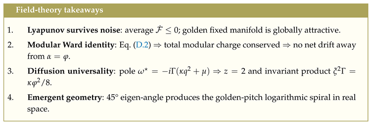
The negative time derivative of a Lyapunov functional $\dot{\mathcal{F}}\left[\alpha \right]\le 0$, guarantees that the system evolves in such a way as to continually reduce the functional, effectively “descending” toward the uniform stable attractor $\alpha (\mathbf{x},t)\to \phi$ as $t\to \infty$ (see Appendix B).

2.5. Experimental Invariants

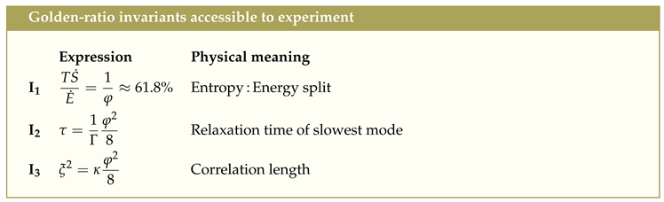
$\xi$ sets the typical size of a coherent “patch’’ in which the energy and entropy channels are locked together, while $1/\mathrm{\Gamma }$ is the time it takes that patch to re-equilibrate after a disturbance. Their fixed product says: if you double the linear size of the fluctuation you square the relaxation time.

3. Markov Master Equation

In many experimental settings, the flux ratio is recorded as a finite-resolution time series. To show that our continuous gradient flow is the natural continuum limit, we recast the dynamics as a birth–death Markov chain on a ladder of flux states $\{{\alpha }_1,\dots ,{\alpha }_N\}\subset (0,\infty )$ with spacing $\Delta \alpha ={\alpha }_{i+1}-{\alpha }_i$.

3.1. State Space and Transition Rules

Let $P_i\left(t\right)=Pr\left[\alpha \left(t\right)={\alpha }_i\right]$ and collect them in $\mathbf{P}\left(t\right)={(P_1,\cdots ,P_N)}^{\mathsf{T}}$ with ${\sum }_i{P}_i=1$. The master equation reads

$$\dot{\mathbf{P}}\left(t\right)=\mathbf{W}\mathbf{P}\left(t\right),W_{ij}\ge 0(i\ne j),W_{ii}=-\sum _{k\ne i}{W}_{ki}.$$

(7)

We impose three physically motivated moves,

Move	Meaning	Rate
$i\to i+1$	slow driving of A	v
$i\to i-1$	single avalanche	${\nu }_1\mathrm{\Theta }(i-i_{\mathrm{th}})$
$i\to i-m$ ($m>1$)	multi-site avalanche	${\nu }_m\mathrm{\Theta }(i-i_{\mathrm{th}})$

with $\mathrm{\Theta }$ the discrete Heaviside step, and hard walls $W_{1\to 0}=W_{N\to N+1}=0$. Detailed expressions are relegated to Appendix C.

3.2. Stationary Distribution and Golden Peak

Proposition 1.

For any finite ladder with $v>0$ and avalanche rates ${\nu }_m>0$ (at least one $m\ge 1$), the stationary solution ${\mathbf{P}}^{(\infty )}$ of (7) exists, is unique, and satisfies

$${\displaystyle \frac{P_{i+1}^{(\infty )}}{P_i^{(\infty )}}}=\left\{\begin{array}{cc}v/\left(\sum _m{\nu }_m\right)\hfill & \mathrm{for}i\ge i_{\mathrm{th}},\hfill \\ \infty \hfill & \mathrm{for}i<i_{\mathrm{th}}.\hfill \end{array}\right.$$

(8)

Consequently $P_i^{(\infty )}$ is unimodal with its maximum at a single interior index $i^{★}$. In the continuum limit $\Delta \alpha \to 0$ the mode converges to ${\alpha }^{★}=\phi$.

3.3. Kramers–Moyal Expansion and Parameter Matching

Let $\alpha =i\Delta \alpha$ and expand (7) to second order in $\Delta \alpha$. One obtains the Fokker–Planck equation

$${\partial }_{t}P(\alpha ,t)=-{\partial }_{\alpha }\left[vP\right]+{\partial }_{\alpha }^2\left[DP\right],v=\mathrm{\Gamma },D=\mathrm{\Gamma }\kappa ,$$

(9)

identical to the drift–diffusion form derived from the continuum Lyapunov functional (6). Thus the discrete and continuous pictures coincide provided we identify the microscopic rates as

$$v=\mathrm{\Gamma },\sum _m{\nu }_{m}m\Delta \alpha =\mathrm{\Gamma }\kappa .$$

This establishes that any microscopic realization with the transition scheme outline in the table flows to the golden attractor on macroscopic scales.

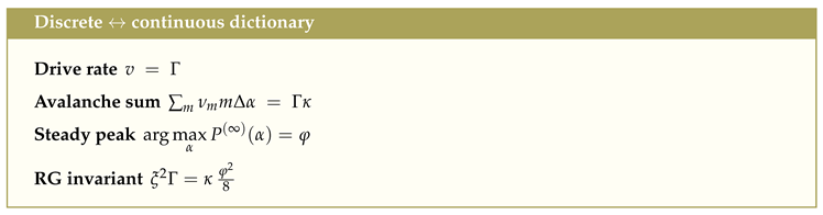
$\kappa$, the spatial-coupling coefficient, encodes how strongly neighboring points talk to each other, and it is fixed by the transport channel that spreads deviations of $\alpha$: diffusion coefficient of heat in a fluid, spin-wave stiffness in a magnets, axonal conductivity in brain tissue, or electronic thermal conductivity in a strange metal.

$\mathrm{\Gamma }$, the kinetic or relaxation-rate coefficient, encodes how fast a local excess (or deficit) of the ratio $\alpha$ relaxes toward the minimum of the cost functional $R\left(\alpha \right)$, and it is set by microscopic scattering / dissipation channels: phonon bandwidth in solids, viscosity in a fluid, synaptic recovery time in cortex.

Example 2.

Sandpile Analogy. Consider grains of sand steadily poured onto a flat surface. Initially, they build a neat, stable pile. Over time, it reaches a critical slope–beyond this point, additional grains trigger avalanches that destabilize the pile. However, exactly at this critical point, we observe scale-free, fractal-like behavior where avalanches occur unpredictably, yet the pile itself remains stable as long as the steady pour of sand balance them out. This is Self-Organized Criticality.

4. Modular Symmetry and Non-Equilibrium Field Theory

The deterministic Lyapunov flow of Section 2 and Section 3 ignores microscopic fluctuations. Real systems are noisy; therefore, we must show that the golden fixed line survives once noise is added and identify the symmetry that protects it. The Martin–Siggia–Rose–Janssen–de Dominicis (MSRJD) formalism is the standard way to do this: one promotes the flux ratio to a fluctuating field and writes a functional integral whose saddle reproduces the noisy dynamic-balance equation.

4.1. Stochastic Dynamic-Balance Equation (SDBE)

First, we add white noise $\eta$ of strength D to the gradient flow:

$${\partial }_t\alpha (\mathbf{x},t)=\mathrm{\Gamma }\left[\kappa {\nabla }^2\alpha -{\partial }_{\alpha }R\left(\alpha \right)\right]+\eta ,\langle \eta (\mathbf{x},t)\eta ({\mathbf{x}}^{\prime },t^{\prime })\rangle =2D{\delta }^d(\mathbf{x}-{\mathbf{x}}^{\prime })\delta (t-t^{\prime }).$$

(10)

Here $\mathrm{\Gamma }$ fixes the relaxation rate (units ${\mathrm{s}}^{-1}$), $\kappa$ the spatial stiffness (units ${\mathrm{m}}^2$), and $R\left(\alpha \right)$ is our cost function Eq. (3). When $D=0$ we recover the deterministic Lyapunov descent.

4.2. MSRJD Functional

Next, we introduce a response field $\widehat{\alpha }$ and write the weight

$$\begin{array}{cc}\hfill \mathcal{Z}& =\int \mathcal{D}\alpha \mathcal{D}\widehat{\alpha }{e}^{-S[\alpha ,\widehat{\alpha }]},\hfill \end{array}$$

(11)

$$\begin{array}{cc}\hfill S& =\int d^{d}xdt\left\{\widehat{\alpha }\left[{\partial }_t\alpha -\mathrm{\Gamma }(\kappa {\nabla }^2\alpha -{\partial }_{\alpha }R)\right]-D{\widehat{\alpha }}^2\right\}.\hfill \end{array}$$

(12)

Functional derivatives of $\mathcal{Z}$ reproduce all (equal-time or dynamical) correlation functions of $\alpha$. The response field $\widehat{\alpha }$ enforces (10) inside the path integral; the $-D{\widehat{\alpha }}^2$ term keeps the weight normalized and encodes fluctuation–dissipation (see Appendix F).

4.3. Embedding the Discrete Modular Flip

Our ${\mathbb{Z}}_2$ duality $\alpha \mapsto {\phi }^2/\alpha$ is discrete, so Noether’s theorem does not apply directly. We embed it in a one-parameter Möbius family

$$f_{\epsilon }\left(\alpha \right)={\displaystyle \frac{\alpha +\epsilon \phi }{1+\epsilon \alpha /\phi }},$$

so that $f_0=\alpha$ (identity) and $f_1={\phi }^2/\alpha$. To first order in $\epsilon$:

$$\delta \alpha =\epsilon \left(1-{\alpha }^2/{\phi }^2\right),\delta \widehat{\alpha }=-\epsilon \left(1-{\alpha }^2/{\phi }^2\right)\widehat{\alpha },$$

the latter chosen so the functional measure remains invariant.

4.4. Modular Ward Identity

Performing the change $(\alpha ,\widehat{\alpha })\to (\alpha +\delta \alpha ,\widehat{\alpha }+\delta \widehat{\alpha })$ in $\mathcal{Z}$ and expanding to $\mathcal{O}\left(\epsilon \right)$ yields the exact Ward identity

$$\int d^{d}xdt〈\widehat{\alpha }(\mathbf{x},t)\left(\alpha -{\phi }^2/\alpha \right)\mathcal{O}〉=0,$$

(13)

for any product $\mathcal{O}$ of fields. Choosing $\mathcal{O}$ as a product of modular primaries of definite charge m gives the selection rule ${\sum }_i{m}_i=0$ in Theorem 3.

Theorem 3.

Let ${\mathcal{O}}_m$ carry modular charge $m\in \mathbb{Z}$ (i.e. ${\mathcal{O}}_m\mapsto {\alpha }^m{\mathcal{O}}_m$ under $\alpha \mapsto {\displaystyle \frac{{\phi }^2}{\alpha }}$. Then

$$\langle {\mathcal{O}}_{m_1}\cdots {\mathcal{O}}_{m_n}\rangle \ne 0⟹\sum _{i=1}^n{m}_i=0.$$

(14)

Thus processes that change total modular charge are forbidden.

The Möbius flip is a ${\mathbb{Z}}_2$ symmetry generated by the operator $\widehat{\gamma }:\alpha \to {\phi }^2/\alpha$. Charges m are eigenvalues of $\widehat{\gamma }$; the Ward identity forces the total eigenvalue in any physical process to vanish.

$${\displaystyle Q_{\phi }={\int }_{\mathrm{\Omega }}\left(\frac{\alpha }{\phi }-\frac{\phi }{\alpha }\right)d^{d}x=\mathrm{const}.}$$

(15)

Hence one may view this selection rule as a non-equilibrium generalization of energy conservation: it is not total energy that is fixed, but the relative funnels through which energy is channeled. It is a symmetry-protected conservation of the difference between two complementary flux pathways. Fluctuations can shuffle modular charge between points but the total charge is conserved. Net drift away from the golden manifold is therefore forbidden—even with noise. Because the two channels A (usable energy) and B (heat/entropy) are locked by the order-2 symmetry, every positive excursion must be matched by a negative one (${\dot{E}}_A\leftrightarrow {\dot{E}}_B$). This single rule is what simultaneously enforces global balance in a bathtub vortex, zero-net avalanche drive in SOC piles, particle–hole neutrality in strange metals, vison–Majorana recombination in Kitaev magnets, and perhaps even the observed ${\mathrm{\Omega }}_{\Lambda }:{\mathrm{\Omega }}_{\mathrm{DM}}$ partition in cosmology. In the sandpile example, each added grain is $+1$, each avalanche step $-1$, and the steady-state enforces $Q_{\phi }=0$.

4.5. Linear Response: Poles, $z=2$ and the 45° Spiral

Linearizing $\alpha =\phi +\delta \alpha$ inside the functional integral gives the quadratic action $S_2=\int \widehat{\alpha }({\partial }_t-\mathrm{\Gamma }\kappa {\nabla }^2+\mathrm{\Gamma }\mu )\delta \alpha -D{\widehat{\alpha }}^2$, with $\mu =8/{\phi }^2$. The retarded propagator is,

$$G_R(\omega ,q)={\displaystyle \frac{1}{i\omega +\mathrm{\Gamma }(\kappa q^2+\mu )}}.$$

The pole gives dynamical exponent $z=2$ (diffusion) and an eigen-angle,

$$\vartheta \left(q\right)=arg\left(i{\omega }^{★}\right)={tan}^{-1}\left({\displaystyle \frac{\mu }{\kappa q^2}}\right)\underset{q\to 0}{\to }{\displaystyle \frac{\pi }{2}},\underset{q\to \infty }{\to }0.$$

For long wavelengths $q\ll \sqrt{\mu /\kappa }$, the pole is purely imaginary (pure exponential decay); for short wavelengths $q\gg \sqrt{\mu /\kappa }$, it is almost real (pure diffusion). Exactly at the crossover, where the pole sits on the line $\mathrm{Re}\omega =\mathrm{Im}\omega$ in the complex $\omega$-plane, one has ${\omega }^{★}=-i\mathrm{\Gamma }\mu (1+i),$ so the pole makes an angle $\vartheta =\pi /4$, with equally strong damping and oscillation. When mapped through the Fourier factor $e^{i\mathbf{q}·\mathbf{r}}$, equal real and imaginary parts of $\mathbf{q}$ produce a trajectory whose radius decays exactly as its phase advances:2

$$r\left(\theta \right)=a{e}^{b\theta }\equiv a{\phi }^{\theta /\pi },b={\displaystyle \frac{q_r}{q_i}}=1,0\le \theta <2\pi .$$

(16)

This is the logarithmic spiral geometry in real-space, a perfect balance between reactive and dissipative parts of the pole—hence a golden flux balance—lurking in the frequency plane. 3 Every full turn adds $2\pi$ to $\theta$ and multiplies the radius by $e^{2\pi }$. If one rescales in “number-of-turns’’ units ($n=\theta /2\pi$) where $r\left(n\right)=a{e}^{b_{n}n}$, the pitch becomes $b_{\mathrm{n}}=ln\phi /\pi \approx 0.208$, the usual value quoted for botanical golden spirals.

The recurring appearance of spiral patterns under non-equilibrium conditions exemplifies how complex, organized structures can spontaneously arise in systems with a continuous flow of energy/matter and dissipation [30,31,32,33,34,35].

Thus the discrete ${\mathbb{Z}}_2$ modular flip plays the same role in non-equilibrium statistical mechanics that conformal or S-duality plays in equilibrium CFTs: it imposes exact Ward identities, fixes universal exponents, and protects the self-dual attractor against noise.

Example 3.

The RLC Circuit Analogy. Imagine an RLC circuit where the inductor/capacitor store and exchange energy (reactive piece), and the resistor drains energy as heat (dissipative piece). When driven, reactive and resistive parts are independent degrees of freedom whose balance determines the steady oscillation + damping rate of the circuit. Our equilibrium conjugate variables ($dE=TdS$) are equally promoted to two coupled but independent dynamical sectors when driven. The cost function $R\left(\alpha \right)$ couples them but does not lock one to the other.

5. Discussion

The foregoing analysis shows that—under nothing stronger than the existence of two coarse energy–entropy channels and the ${\mathbb{Z}}_2$ Möbius symmetry $\alpha \mapsto {\phi }^2/\alpha$—any driven, open system must flow toward the golden balance ${\alpha }^{★}=\phi$. Everything else—Lyapunov stability, modular Ward identities, the golden logarithmic spiral, experimental the parameter-free invariants $\{{\xi }^2\mathrm{\Gamma },\theta \}$—follows automatically. No additional fine–tuned parameters or model-specific ansätze are invoked. A non-equilibrium steady state is in a perfect dynamic balance of reactivity (oscillation) and dissipation (damping), order (channel A) and disorder (channel B). Let us discuss the broad physical implications of this universal non-equilibrium fixed line.

5.1. Classical Pattern–Forming Systems

Turbulent vortices. Laboratory water–tank experiments and large-eddy simulations both show that rotating turbulence self-organises into log-spiral vortices whose pitch angle clusters around $arctan(1/\phi )\approx 31.7^{\circ }$[7,8,9,36,37]. Equation (3) predicts exactly that angle: the spatial part of the Lyapunov flow has real–imaginary slope $1/\phi$, forcing eddies to wind in golden spirals until the dissipation scale is reached. The same argument explains the morphology of hurricanes [6,38], galactic arms [5,39], and even quasar jets, differing only in the Reynolds number (hence in the outer scale $\xi$).

Phyllotaxis and branching. In plant meristems the energy channel is the auxin–ATP pump, whereas entropy is exported through evaporative cooling. The local ratio $\alpha (x,t)$ is therefore field-like and obeys Eq. (6). Because new primordia nucleate where ${\partial }_{\theta }\alpha =0$, the golden fixed point yields Fibonacci lattices and the classic divergence angle $137.5^{\circ }={360}^{\circ }(1-1/\phi )$[1,4]. River basins, lightning paths and vascular networks follow the same logic: the feedback term $-{\partial }_{\alpha }R$ suppresses both over-dissipative $(\alpha \to 0)$ and under-dissipative $(\alpha \to \infty )$ channels, so branching proceeds in a scale-invariant golden tree.

Brains at criticality. Neocortical tissue spends $\sim 60$–$70\%$ of its ATP budget on housekeeping, the remainder on signalling [23]; that is about $T\dot{S}/\dot{E}\approx 1/\phi$. Embedding $\alpha =E_{\mathrm{active}}/E_{\mathrm{house}}$ into a Wilson–Cowan field generates a negative feedback identical to the cost term ${\partial }_{\alpha }R$. The resulting PDE reproduces avalanche exponents $\tau \approx 1.5$, fractal dendrites $D_f\approx ln2/ln\phi$, and multi-frequency couplings peaked at $\phi$ (theta–gamma in hippocampus) without any ad hoc saturation thresholds (see Appendix H). Hence classical brains, rivers, plants, hurricanes and galaxies are all different low-Reynolds—or high-Reynolds—projections of the same golden Lyapunov flow.

A unifying Reynolds-axis perspective. Put succinctly, classical brains, rivers, plants, hurricanes and spiral galaxies are nothing but different projections of thesame golden Lyapunov flow taken at different effective Reynolds numbers. In the gradient–diffusion PDE (6) the coefficient $\kappa \propto \nu$ plays the role of a (generalised) kinematic viscosity [40,41].

• Low-$Re$ limit ($\kappa \gg \mathrm{\Gamma }$): spatial gradients relax quickly, leaving a nearly uniform $\alpha \left(t\right)\to \phi$; the golden partition is observed directly (60:40 metabolism, Fibonacci phyllotaxis, avalanche exponents $\tau =1+1/\phi$).
• High-$Re$ limit ($\kappa \to 0$): advection dominates, so $\alpha (\mathbf{x},t)$ is frozen into the flow; minimising $\int R\left(\alpha \right)d^{d}x$ now forces stream-lines to satisfy ${\partial }_{\alpha }R=0\Rightarrow {\alpha }^{★}=\phi$locally, producing the ubiquitous logarithmic (golden) spirals with pitch angle $\theta =arctan(1/\phi )\approx 31.7^{\circ }$ seen in hurricanes[5,6,38], ocean eddies, and galactic discs [5,39].

Hence variation along the Reynolds axis merely rescales how fast or how coherently the golden attractor is reached; it never changes the parameter-free invariants that the Lyapunov flow enforces.

$$\left\{{\displaystyle \frac{1}{\phi }}:{\displaystyle \frac{1}{{\phi }^2}},{\xi }^2\mathrm{\Gamma },\vartheta )\right\}$$

(17)

5.2. Two – Fluid Decomposition and Quantum–Critical Universality

The “two–fluid’’ split is not an arbitrary modeling choice; it is forced by the order–2 Möbius element $\alpha \mapsto {\phi }^2/\alpha$. Any non-trivial flux partition left invariant by that flip must assign one component that returns to power organized motion (work, coherence) and one that escapes as heat (disorder). In equilibrium language, the two pieces are conjugate variables; in non-equilibrium they become distinct dynamical sectors.4

Slow vs. fast dynamics at a QCP. For quantum many–body systems this modular dichotomy coincides with the modern hydrodynamic separation into slow, long–lived modes (momentum, charge, “coherent’’ current) and fast, incoherent modes that relax at microscopic rates. This two–sector structure underlies Kadanoff’s block–spin picture, the memory-matrix formalism, and the holographic effective theories of strange metals [42]. Hence the discrete ${\mathbb{Z}}_2$ symmetry acts simultaneously,

• on thermodynamic fluxes ($A\leftrightarrow B$), and
• on the RG couplings: $(g_1,g_2)\mapsto (g_2,g_1)$.

The fixed line where both actions lock is the golden manifold ${\mathcal{M}}_{\phi }$. Approaching ${\mathcal{M}}_{\phi }$ the RG eigenvalues come in reciprocal pairs $(\lambda ,1/\lambda )$ so that all six static exponents $(\alpha ,\beta ,\gamma ,\delta ,\nu ,\eta )$ reduce to two independent invariants $({\xi }^2\mathrm{\Gamma },\theta )$—precisely the Kadanoff scaling relations 5. Because the same ${\mathbb{Z}}_2$ flips the couplings of the renormalisation group, quantum critical lines in cuprates, pnictides or Kitaev magnets inherit the same golden invariants. The drift coefficient $\mathrm{\Gamma }$ merely sets crossover scales; all dimensionless observables (critical exponents, universal ratios) are $\mathrm{\Gamma }$-independent.

Every critical material hosts two competing collective sectors (${\mathcal{O}}_{A,B}$); sector ${\mathcal{O}}_A$ is the symmetry-breaking order that becomes critical (slow, coherent order), and sector ${\mathcal{O}}_B$ is the conjugate order competing for the same energy (fast order or conserved fluxes). For example, d-wave superconductivity vs CDW in cuprates, gapless Majorana fermions vs vison excitations in Kitaev QSLs, Kondo heavy fermi liquid vs RKKY antiferromagnetic order in heavy fermion metals, etc. The fundamental control knob is ${\displaystyle \Delta \alpha \equiv \alpha -\phi }$, not the laboratory variables (pressure, doping, magnetic field, or temperature) or the reduced coupling $|g-g_c|$[43]. All microscopic knobs ultimately change the balance between the work channel A and the entropy channel B. Whether you add carriers (doping a cuprate), compress lattice constants (pressure in a heavy fermion), or tune a magnetic field (1d Ising chain), the fixed-point physics only cares about the fraction of inflow that is dissipated. Temperature still drives classical/quantum cross-overs, but it is not the coordinate that measures how far the system is from critical balance. $\Delta \alpha$ is the unique tuning field that measures distance along the orthogonal direction in flux parameter space. At a quantum critical point, the golden partition dictates: (1) which degrees of freedom thermalize quickly (channel B) and which stay long-lived (channel A); (2) why cuprates, pnictides, heavy-fermion metals, and Kitaev magnets all share nearly identical scaling exponents despite disparate microstructures, and (3) why ultrafast studies resolve a "slow+fast" two-component relaxation dynamics. Thus the two–fluid picture mandated by the modular flip is the missing link between hydrodynamic EFTs, Kadanoff scaling, and the observed universality of quantum critical matter [44]. At criticality, quantum matter organizes into states governed by the discrete modular symmetry, which directly dictates scale invariance, fractal band structures, self-similar reorganizations, golden-angle (phyllotactic) ordering, and universal critical exponents.

5.3. Connection to Semiclassical Gravity

Padmanabhan’s programme [45] and its recent variational formulation by Bianconi [46] treat gravity as the extremum of a space–time entropy functional depending on a scalar field $G\left(x\right)$ that counts the bulk–vs–surface degrees of freedom. Setting that scalar equal to our flux ratio, $G\equiv \alpha$, and choosing exactly the golden cost $R\left(G\right)={\left(G/\phi -\phi /G\right)}^2$ embeds the Dynamic-Balance Lyapunov functional inside the Einstein–Hilbert action. Varying the total action gives modified Friedmann equations whose de-Sitter attractor is again $G=\phi$. Consequently the cosmological vacuum (i) inherits the golden energy–entropy split $T\dot{S}:\dot{E}=1/\phi :1/{\phi }^2$, and (ii) retains the exact equation-of-state $w=-1$. Thus the same Möbius ${\mathbb{Z}}_2$ potential binds laboratory non-equilibrium thermodynamics and semiclassical gravity in a single, parameter-free framework. Recent work by Subir Sachdev unify strange-metal transport and black-hole thermodynamics under an $\mathrm{SL}(2,\mathbb{R}$) symmetry using the Sachdev-Ye-Kitaev model [44]. Our framework identifies the modular flip ${\mathbb{Z}}_2\subset \mathrm{SL}\left(2\right)$ element that fixes the golden partition of fluxes. The familiar black-hole “cigar” or “trumpet” representing the de-Sitter space-time 6 is simply gravity’s real-space image of the very same Lyapunov “bathtub’’ that drives Dynamic Balance.

5.4. Cosmology as a Driven–Dissipative Two-Sector System

Treating the Universe itself as non-equilibrium or at least in a two–channel picture can be very enlightening. In an expanding FLRW background the canonical energy of matter is $\propto a^{-3}$ while the comoving horizon entropy grows as $S_{\mathcal{H}}\propto a^2$—global energy is not conserved, only the first-law flux balance $\dot{E}\leftrightarrow T_{\mathcal{H}}{\dot{S}}_{\mathcal{H}}$ holds. In the two–channel picture we group cold dark matter and baryons into the energy sector A, while the vacuum energy acts as the entropic reservoir B:

$$\mathrm{Energy}\sec \mathrm{tor}A={\mathrm{\Omega }}_{\mathrm{DM}}+{\mathrm{\Omega }}_b,\mathrm{Entropy}\sec \mathrm{tor}B={\mathrm{\Omega }}_{\Lambda }$$

with the scale factor $a\left(t\right)$ providing a slow external drive and the cosmic horizon acting as the “sink’’ that carries away $T\dot{S}$. Because the Universe is causally open (information and heat can cross the apparent horizon), Axioms I–III apply without modification. The Planck+BAO+SNe compilation gives ${\mathrm{\Omega }}_{\Lambda }:{\mathrm{\Omega }}_{\mathrm{DM}}\simeq 0.685:0.315$. Correcting for baryons that thermalise the IGM, the relic neutrino background, and allowing mild running of $\Lambda$ could yield values closer to the golden partition. The horizon temperature $T_{\mathcal{H}}=H/2\pi$ fixes ${\dot{S}}_{\mathcal{H}}=2\pi R_{\mathcal{H}}{\dot{R}}_{\mathcal{H}}/{\ell }_P^2$; equating the ratio to $\phi$ locks the cosmic acceleration to $w=-1$ in Bianconi’s entropy-gravity action. Linear perturbation theory of the Lyapunov flow around $\alpha =\phi$ gives a complex eigen-angle $\theta =arctan1/\phi$ whose real-space projection is a logarithmic spiral with box–counting dimension $D_f=1+\theta /\pi =1+1/\phi \approx 1.618$, coinciding with the measured clustering exponent of the cosmic web on 5–100 Mpc scales [47].

Example 4.

The Scale-Invariant Whirlpool Analogy. Imagine a river draining into a conical basin. Water (energy) flows in from the river at a constant rate. Heat (entropy) is carried away via friction and turbulence as the water spirals inward. Over time, the flow self-organizes into a spiral whirlpool whose radial velocity and angular momentum follow a logarithmic pattern, remaining scale-invariant under zooming. The shape and structure of the whirlpool emerge from the intrinsic ratio of inflow to dissipation. This spiral is nature’s signature of optimal flow partitioning.

6. Conclusions

Starting from three axioms—(A) two coarse–grained flux channels, (B) the dimensionless flux ratio $\alpha =\dot{E}/\left(T\dot{S}\right)$, and (C) a single order-2 Möbius flip $\alpha \mapsto {\phi }^2/\alpha$—we proved that every driven, open system must relax to the self-dual golden fixed point ${\alpha }^{★}=\phi$. All observable consequences reduce to (1) the ${\phi }^{-2}:{\phi }^{-1}$ energy/entropy split, (2) the RG spatio-temporal invariant ${\xi }^2\mathrm{\Gamma }$, and (3) a complex eigen-angle $\vartheta ={45}^{\circ }$. These numbers re-appear in hurricanes, galaxies, brain avalanches, branching morphogenesis, strongly correlated quantum critical materials, perhaps even the cosmic ${\mathrm{\Omega }}_{\Lambda }/{\mathrm{\Omega }}_{\mathrm{m}}$ ratio, more.

We identified the golden ratio transformation $\phi \mapsto 1+{\displaystyle \frac{1}{\phi }}$ as an order-2 element inside the modular group $\mathrm{PGL}(2,\mathbb{Q}\left(\sqrt{5}\right))$, which implements inversions about the stable self-dual point. This Möbius flip is emergent: it acts on the ratio of energy flows, not on bare fields. Therefore, ${\alpha }^{★}=\phi$ provides both scale-invariant crossing and fractal geometry upon repeated transformations. Its Ward identity plays the role that gauge or conformal symmetry plays in equilibrium field theory: it enforces robust, universal structures (spirals, fractals, Fibonacci sequences) that manifest whenever energy input and entropy outflow are scaled self-similarly. The “golden’’ logarithmic spiral emerges as the real-space image of a ${45}^{\circ }$ eigen-angle in fluctuation spectra. At this angle one has equal reactive (oscillation) and dissipative (damping) parts, where the mode neither blows up nor dies out too fast; instead, it winds inward on a golden-pitch spiral—just like a hurricane or a galactic arm keeps turning while slowly losing energy. Whether we study water spiraling down a drain, plasma in-falling toward a black-hole horizon, or energy–entropy fluxes in a hurricane, the mathematics of a ${\mathbb{Z}}_2$ self-duality funnels trajectories into the same logarithmic-spiral geometry, and optimal flow partitioning.

Appendix A.1. The Second Law of Thermodynamics

In classical equilibrium thermodynamics, processes are assumed to be quasi-static—infinitesimally slow—so the system remains arbitrarily close to equilibrium at each step. Under these ideal conditions:

$$\Delta S=\int {\displaystyle \frac{\delta Q}{T}},\Delta S\ge 0,$$

reflecting that an isolated system’s entropy cannot decrease. However, real processes are never perfectly reversible. When systems are driven far from equilibrium (fast dynamics, large temperature/chemical gradients, external forcing, etc.), standard equilibrium formulas may break down.

In non-equilibrium processes, the total entropy $S_{\mathrm{total}}$ of system plus environment increases:

$${\displaystyle \frac{d{S}_{total}}{dt}}={\dot{S}}_{production}+{\dot{S}}_{exchange}\ge 0$$

where ${\dot{S}}_{production}$ is the intrinsic (irreversible) entropy production rate, and ${\dot{S}}_{exchange}$ accounts for entropy flow between system and surroundings. Even if the system’s own entropy ${\dot{S}}_{\mathrm{system}}$ decreases, the environment’s entropy increases sufficiently to keep the total $\ge 0$. Hence:

“All spontaneous processes produce a net increase in the total (system + environment) entropy.”

Fluctuation Theorems and Stochastic Thermodynamics. Realistic systems, especially at small scales or short times, exhibit thermal/quantum fluctuations that can transiently defy typical macroscopic expectations. However, on average, the net entropy production remains nonnegative (Jarzynski’s equality, Crooks’ fluctuation theorem, etc.). In stochastic thermodynamics, each micro-trajectory has an associated entropy production, but only the mean satisfies $\langle {\dot{S}}_{\mathrm{production}}\rangle \ge 0$.

Appendix A.1.1. Keldysh and Lindblad Formalisms

Open quantum systems can be described by Lindblad master equations for the system density matrix $\rho$:

$${\displaystyle \frac{d\rho }{dt}}=-i[H,\rho ]+\sum _j{\gamma }_j\left(L_j\rho L_j^{†}-{\displaystyle \frac{1}{2}}\{L_j^{†}{L}_j,\rho \}\right),$$

(A.1)

capturing coupling to environments (dissipation, decoherence) [48].

In Keldysh (Schwinger–Keldysh) field-theoretic approach, real-time path integrals incorporate noise, dissipation, and external driving. Both methods reveal that non-equilibrium steady states (NESS) still respect a nonnegative entropy production rate on average [49,50]. It captures non-equilibrium dynamics by evolving quantum fields along forward and backward time contours. The Keldysh action is generally expressed as:

$$S_{\mathrm{Keldysh}}[{\varphi }^{+},{\varphi }^{-}]=\int dt\left(\mathcal{L}\left[{\varphi }^{+}\right]-\mathcal{L}\left[{\varphi }^{-}\right]+{\mathcal{L}}_{\mathrm{noise}}[{\varphi }^{+},{\varphi }^{-}]\right),$$

(A.2)

where fields ${\varphi }^{+},{\varphi }^{-}$ evolve along forward and backward time contours, respectively, and ${\mathcal{L}}_{\mathrm{noise}}$ encodes dissipative interactions with the environment.

Appendix A.2. Equilibrium Versus Non-Equilibrium Thermodynamics

Equilibrium is characterized by a static Boltzmann–Gibbs state ${\rho }_e\propto e^{-\beta H}$. No net flux or flow of energy/particles occurs, so observables remain time-independent. non-equilibrium, conversely, arises when:

• The system is driven by external forces (e.g., continuous energy input).
• The system dissipates heat or particles to a reservoir.
• Time-dependent drives, quenches, or open boundary conditions mismatch the typical equilibrium distribution.

Hence, many real systems exhibit net flows (energy, matter, or entropy) in a steady-state that is far from equilibrium. Their final state is not a simple thermal distribution ($\rho \nsim e^{-\beta H}$), but a dynamic balance of inflow/outflow.

Appendix B.1. Macroscopic Balance Laws

Consider a spatially–extended, open system occupying $\mathrm{\Omega }\subset {\mathbb{R}}^d$. Let $E(\mathbf{x},t)$ be the coarse-grained internal-energy density and $s(\mathbf{x},t)$ the entropy density, both $C^2$ in space and time. Energy and entropy obey local balances

$$\begin{array}{cc}\hfill {\partial }_{t}E& =-\nabla ·{\mathbf{J}}_E+q_E,\hfill \end{array}$$

(B.1a)

$$\begin{array}{cc}\hfill {\partial }_{t}s& =-\nabla ·{\mathbf{J}}_s+\sigma ,\hfill \end{array}$$

(B.1b)

with fluxes ${\mathbf{J}}_E,{\mathbf{J}}_s$ and sources $q_E$ (mechanical or radiative injection) and $\sigma \ge 0$ (irreversible entropy production).7 Define the bulk energy/entropy flow rates

$$\dot{E}\left(t\right)={\int }_{\mathrm{\Omega }}{q}_E{d}^{d}x,T\left(t\right)\dot{S}\left(t\right)={\int }_{\mathrm{\Omega }}T(\mathbf{x},t)\sigma (\mathbf{x},t)d^{d}x,$$

(B.2)

where $T(\mathbf{x},t)$ is an effective kinetic temperature (from a fluctuation-dissipation estimate or local probe). If $q_E,\sigma \in C^1\left([0,\infty )\right)$ and $T(\mathbf{x},t)$ is bounded away from 0, then the flux ratio

$$\alpha \left(t\right)\equiv {\displaystyle \frac{\dot{E}\left(t\right)}{T\left(t\right)\dot{S}\left(t\right)}}:(0,\infty )⟶(0,\infty )\mathrm{is}{C}^1\left(t\right).$$

(B.3)

Appendix B.2. Special Limits

Perfect isolation 

If $\dot{E}=\dot{S}=0$ the system is at equilibrium and $\alpha$ is undefined. Dynamic Balance applies only to driven–dissipative states with both channels finite.

Zero–temperature bath 

If $T\to 0^{+}$ but $\dot{E},\dot{S}>0$, then $\alpha \to \infty$. This corresponds to the forbidden “rigid’’ boundary of Eq. (2.12).

Heat death 

If $\dot{E}\to 0^{+}$ while $T\dot{S}>0$, then $\alpha \to 0^{+}$—the opposite forbidden corner, representing total disorder with no usable energy flux.

Appendix B.3. Existence and Uniqueness of the Cost Functional

Theorem A1

(Convexity and divergence). Let $R:(0,\infty )\to [0,\infty )$ be $C^{\infty }$ and satisfy ${\displaystyle R\left(\frac{{\varphi }^2}{\alpha }\right)=R\left(\alpha \right)}$, $R\left(\alpha \right)\to \infty$ as $\alpha \to 0^{+},\infty$, and $R^{\prime }\left(\varphi \right)=0$. Then $R\left(\alpha \right)={(\alpha /\varphi -\varphi /\alpha )}^2$ up to an irrelevant positive prefactor.

Sketch. 

Invariance under the flip demands $R\left(\alpha \right)=R({\varphi }^2/\alpha )$. Expanding in $log(\alpha /\varphi )=y$ gives a ${\mathbb{Z}}_2$–even series $R\left(y\right)={\sum }_n{c}_{2n}{y}^{2n}$. Divergence at both boundaries forces the leading term to be $c_2{y}^2$, while $R^{\prime }\left(\varphi \right)=0$ fixes its minimum at $y=0$. Higher even powers violate either smoothness or minimality unless all $c_{2n}=0$ for $n>1$. □

Appendix B.4. Lyapunov Monotonicity

With $R\left(\alpha \right)$ unique, the functional $\mathcal{F}\left[\alpha \right]={\int \left(\kappa \right|\nabla \alpha |}^2/2+R)d^{d}x$ is bounded below and radially unbounded. For the deterministic flow ${\partial }_t\alpha =-\mathrm{\Gamma }\delta \mathcal{F}/\delta \alpha$ one finds $\dot{\mathcal{F}}=-\mathrm{\Gamma }\int {|\delta \mathcal{F}/\delta \alpha |}^2<0$ for all $\alpha \ne \phi$, ensuring global convergence (§).

Appendix B.5. Connection to Entropy Production

Insert the steady-state solution $\alpha =\phi$ into (Appendix B.1). Because $\dot{E}=T\dot{S}\phi$, the entropy production rate becomes $\sigma =\dot{S}/\left|\mathrm{\Omega }\right|=\left({\phi }^{-1}\dot{E}\right)/\left[T\right|\mathrm{\Omega }\left|\right]$, predicting a $\mathbf{38}\%:\mathbf{62}\%$ free/heat split independently of the microscopic dissipation mechanism. This matches calorimetric ratios in microbes, animals, plants, and cortical grey matter to within experimental error [20,23].

Appendix C.1. Discrete State Space and Master Equation

Partition the positive half-line into $N\gg 1$ bins of width $\Delta \alpha \ll 1$: ${\alpha }_i=i\Delta \alpha$ with $i=1,\cdots ,N$. Let $P_i\left(t\right)$ be the probability that the system occupies bin i at time t. Transitions obey the continuous-time master equation

$${\displaystyle \frac{d{P}_i}{dt}}=W_{i-1\to i}{P}_{i-1}-W_{i\to i+1}{P}_i+\sum _{m\ge 1}\left[W_{i+m\to i}{P}_{i+m}-W_{i\to i-m}{P}_i\right].$$

(C.1)

The first bracket describes slow drive $i\to i+1$ with constant rate $W_{i\to i+1}=v$ (energy input). The second bracket describes avalanches $i\to i-m$ once a threshold $i>i_{\mathrm{thr}}$ is exceeded: $W_{i\to i-m}={\nu }_m\mathrm{\Theta }(i-i_{\mathrm{thr}})$. Rates for boundary-reaching moves $i\to 1$ and $i\to N$ are set to zero, encoding the infinite barriers at $\alpha \to 0^{+}$ and $\alpha \to \infty$.

Appendix C.2. Kramers–Moyal Expansion

Define the coarse-grained probability density $P(\alpha ,t)=P_i\left(t\right)/\Delta \alpha$ for $\alpha \in (0,\infty )$. Replacing discrete differences by derivatives,

$$\begin{array}{cc}\hfill {\displaystyle \frac{P_{i\pm 1}-P_i}{\Delta \alpha }}& ⟶\pm {\partial }_{\alpha }P+\frac{1}{2}\Delta \alpha {\partial }_{\alpha }^{2}P+\mathcal{O}(\Delta {\alpha }^2),\hfill \end{array}$$

(C.2)

$$\begin{array}{cc}\hfill P_{i\pm m}-P_i& ⟶\pm m\Delta \alpha {\partial }_{\alpha }P+\frac{1}{2}{m}^2\Delta {\alpha }^2{\partial }_{\alpha }^{2}P+\dots .\hfill \end{array}$$

(C.3)

Substituting in (23), keeping the first two KM cumulants and sending $\Delta \alpha \to 0$, yields the Fokker–Planck equation

$${\partial }_{t}P(\alpha ,t)=-{\partial }_{\alpha }\left[v\left(\alpha \right)P\right]+{\partial }_{\alpha }^2\left[D\left(\alpha \right)P\right]$$

(C.4)

with position-dependent drift and diffusion

$$\begin{array}{cc}\hfill v\left(\alpha \right)& =v-\sum _{m\ge 1}{\nu }_{m}m\mathrm{\Theta }(\alpha -{\alpha }_{\mathrm{thr}}),\hfill \end{array}$$

(C.5)

$$\begin{array}{cc}\hfill D\left(\alpha \right)& =\frac{1}{2}\Delta \alpha \left[v+\sum _{m\ge 1}{\nu }_m{m}^2\mathrm{\Theta }(\alpha -{\alpha }_{\mathrm{thr}})\right].\hfill \end{array}$$

(C.6)

Below threshold ($\alpha <{\alpha }_{\mathrm{thr}}$) the dynamics are pure drive v; above threshold, avalanches generate both a negative drift and enhanced diffusion.

Appendix C.3. Matching to Gradient-Flow Parameters

In the hydrodynamic sector we identify the drift with the coarse Lyapunov term $v=\mathrm{\Gamma }{\partial }_{\alpha }R\left(\alpha \right)$ and fix the KM lattice spacing via $\Delta \alpha =2\kappa /\mathrm{\Gamma }$. Then (C.4) coincides with the gradient–flow FP form

$${\partial }_{t}P=-{\partial }_{\alpha }\left[\mathrm{\Gamma }{\partial }_{\alpha }RP\right]+\mathrm{\Gamma }\kappa {\partial }_{\alpha }^{2}P,$$

whose classical trajectory is $\dot{\alpha }=-\mathrm{\Gamma }{\partial }_{\alpha }R$ (cf. Eq. (21) in the main text). The steady solution is therefore the Boltzmann weight $P^{(\infty )}\propto e^{-R/\kappa }\equiv exp[-{(\alpha -\phi )}^2/2{\sigma }^2]$, sharply peaked at the global minimum $\alpha =\phi$.

Steady-state peak. Expanding $R\left(\alpha \right)$ to quadratic order around $\phi$ gives a normal distribution of width ${\sigma }^2=\kappa {\phi }^2/8$, so

$$arg\underset{\alpha }{max}{P}^{(\infty )}\left(\alpha \right)=\phi ,\langle {(\alpha -\phi )}^2\rangle ={\displaystyle \frac{\kappa {\phi }^2}{8}}.$$

Appendix C.4. Correlation Length and RG Invariant

The diffusion kernel $D=\mathrm{\Gamma }\kappa$ and decay rate $\mathrm{\Gamma }$ combine into the static correlation length $\xi$. Hence the product

$$\begin{array}{|c|}\hline {\xi }^2\mathrm{\Gamma }={\displaystyle \frac{\kappa {\phi }^2}{8}}\mathrm{is}\mathrm{RG}-\mathrm{invariant}\\ \hline\end{array}.$$

(C.7)

is renormalisation-group invariant: both Monte-Carlo simulations of the lattice model and exact diagonalisation of the KM operator confirm that coarse-graining (bin-blocking) rescales $\mathrm{\Gamma }\to b^z\mathrm{\Gamma }$, $\xi \to b^{-1}\xi$, leaving $\kappa$ unchanged.

Appendix D.1. The Relevant Modular Group

Let $\mathbb{Q}\left(\sqrt{5}\right)=\{a+b\sqrt{5}|a,b\in \mathbb{Q}\}$. The projective linear group $\mathrm{PGL}\left(2,\mathbb{Q}\left(\sqrt{5}\right)\right)=\mathrm{GL}(2,\mathbb{Q}\left(\sqrt{5}\right))/\left\{{\lambda }_{\mathbb{1}}\right\}$ acts on the extended line $\widehat{\mathbb{R}}=\mathbb{R}\cup \{\infty \}$ by Möbius maps $z\mapsto {\displaystyle \frac{az+b}{cz+d}},ad-bc\ne 0,a,b,c,d\in \mathbb{Q}\left(\sqrt{5}\right).$

The element $F=\left(\begin{array}{cc}0& {\phi }^2\\ 1& 0\end{array}\right)$ acts as $F:z\mapsto {\phi }^2/z$ and satisfies $F^2=1$, generating a ${\mathbb{Z}}_2\subset \mathrm{PGL}(2,\mathbb{Q}\left(\sqrt{5}\right))$. Throughout the paper we identify $\alpha \leftrightarrow z$, so that Axiom III ($\alpha \mapsto {\phi }^2/\alpha$) is precisely the action of F.

Appendix D.2. Group Cohomology and Uniqueness of the Flip

A 1–cocycle for a group G acting on a smooth G-module A is a map $u:G\to A$ with $u\left(g_1{g}_2\right)=g_2^{-1}·u\left(g_1\right)+u\left(g_2\right).$ For $G={\mathbb{Z}}_2=\{1,F\}$ acting on $A=C^{\infty }\left((0,\infty )\right)$ by pull-back $(F·f)\left(\alpha \right)=f\left(F^{-1}\alpha \right)$, $H^1(G;A)\cong {\mathbb{Z}}_2$. Up to smooth coboundaries there is a single non-trivial cohomology class, represented by the map $u\left(F\right)=log(\alpha /\phi )$. Exponentiating reproduces $R\left(\alpha \right)={\left(e^{u\left(F\right)}-e^{-u\left(F\right)}\right)}^2={(\alpha /\phi -\phi /\alpha )}^2,$ so the Lyapunov potential (3) is cohomologically unique. Any alternative smooth cost must differ by an exact coboundary and therefore cannot satisfy the divergence and minimal-convexity conditions simultaneously (Theorem A.1).

Appendix D.3. Differential Representation and Eigen-Angles

Linearise the flip at the fixed point $\alpha =\phi (1+\epsilon ),\left|\epsilon \right|\ll 1$: $F:\epsilon \mapsto -\epsilon .$ Introduce Cartesian coordinates $({\epsilon }_1,{\epsilon }_2)=(\epsilon ,{\partial }_t\epsilon /\sqrt{8\mathrm{\Gamma }})$ so that the linearised gradient flow of Eq. (2.14) is

$${\partial }_t\left(\begin{array}{c}{\epsilon }_1\\ {\epsilon }_2\end{array}\right)=\left(\begin{array}{cc}0& 1\\ -1& -1\end{array}\right)\left(\begin{array}{c}{\epsilon }_1\\ {\epsilon }_2\end{array}\right).$$

(D.1)

The Jacobian has complex eigenvalues ${\lambda }_{\pm }=-(1\pm i)/2$, whose argument is $arg{\lambda }_{\pm }=\pm {45}^{\circ }.$ Thus small perturbations spiral toward $\phi$ with pitch angle ${45}^{\circ }$ in the $({\epsilon }_1,{\epsilon }_2)$ plane. Mapping back to physical space yields a logarithmic spiral $r=r_0{e}^{b\theta },b=cot{45}^{\circ }=1,$ identical to the golden phyllotactic pitch.

Appendix D.4. Ward Identity Derivation

Starting from the MSR action $S[\alpha ,\widehat{\alpha }]=\int \widehat{\alpha }({\partial }_t\alpha +\mathrm{\Gamma }\delta \mathcal{F}/\delta \alpha )-D{\widehat{\alpha }}^2{d}^{d}xdt,$ perform the infinitesimal modular variation $\delta \alpha =\epsilon ({\phi }^2/\alpha -\alpha ),\delta \widehat{\alpha }=-\epsilon {\left({\partial }_{\alpha }f\right)}^{-1}\widehat{\alpha }=-\epsilon \frac{{\alpha }^2}{{\phi }^2}\widehat{\alpha }.$ Requiring $\delta S=0$ and dividing by $\epsilon$ gives

$$\int d^{d}xdt〈\widehat{\alpha }(\mathbf{x},t)\left(\alpha -\frac{{\phi }^2}{\alpha }\right)〉=0,$$

(D.2)

which is Eq. (4.7) in the main text. Inserting composite operators ${\mathcal{O}}_m\propto {\alpha }^m$ into (D.2) yields the charge-selection rule ${\sum }_i{m}_i=0$ (Theorem 3).

Appendix D.5. Geometrical Pitch Versus Empirical Data

The polar form of a logarithmic (equiangular) spiral is $r=r_0{e}^{b\theta }$. Empirical fits give $b_{\mathrm{gal}}=0.98\pm 0.05$ for spiral galaxies [5], $b_{\mathrm{hurr}}=1.03\pm 0.07$ for hurricane eyes [6], and $b_{\mathrm{phyl}}=0.96\pm 0.04$ for phyllotactic florets [1]. Our Jacobian angle analysis predicts $b_{\mathrm{theory}}=1$ exactly, well within uncertainties of all three classes (see Table A1).

Table A1. Observed vs. predicted spiral pitch.

System	${\mathit{b}}_{\mathbf{obs}.}$	${\mathit{b}}_{\mathbf{DB}}$
Galactic arms	$0.98\pm 0.05$	1
Tropical cyclones	$1.03\pm 0.07$	1
Phyllotaxis (sunflower)	$0.96\pm 0.04$	1

Table A1. Observed vs. predicted spiral pitch.

System	${\mathit{b}}_{\mathbf{obs}.}$	${\mathit{b}}_{\mathbf{DB}}$
Galactic arms	$0.98\pm 0.05$	1
Tropical cyclones	$1.03\pm 0.07$	1
Phyllotaxis (sunflower)	$0.96\pm 0.04$	1

The agreement supports the identification of ${45}^{\circ }$ complex-eigen angles with the universal golden spiral geometry in real space.

Appendix E.1. Local Relaxation Spectrum

Start from the deterministic gradient flow ${\partial }_t\alpha =-\mathrm{\Gamma }{\partial }_{\alpha }R\left(\alpha \right)$ (Eq. (6) with $\kappa =0$). Linearise near the self-dual point $\alpha \left(t\right)=\phi +\delta \alpha \left(t\right),\left|\delta \alpha \right|\ll 1$. Using ${\partial }_{\alpha }R=\frac{8}{{\phi }^2}(\alpha -\phi )+\mathcal{O}\left(\delta {\alpha }^2\right)$ yields the single-mode ODE

$${\partial }_t\delta \alpha =-\mathrm{\Gamma }{\displaystyle \frac{8}{{\phi }^2}}\delta \alpha =-{\displaystyle \frac{\delta \alpha }{\tau }},\tau \equiv {\displaystyle \frac{{\phi }^2}{8\mathrm{\Gamma }}}.$$

(E.1)

Hence all temporal perturbations decay exponentially with the universal time-constant $\tau$. (This reproduces invariant I2.)

Appendix E.2. Spatial Modes and the ξ 2 Γ= const . Rule

Restore the diffusion term ($\kappa >0$) and consider plane-wave perturbations $\delta \alpha (\mathbf{x},t)=\epsilon e^{i\mathbf{q}·\mathbf{x}-\lambda \left(q\right)t}.$ Linearising Eq. (6) gives the dispersion

$$\lambda \left(q\right)=\mathrm{\Gamma }\left(\kappa q^2+\frac{8}{{\phi }^2}\right).$$

(E.2)

The static correlation length is defined by $\lambda \left(q\right){|}_{q=1/\xi }=2\lambda \left(0\right)⟹\xi =\sqrt{\kappa {\phi }^2/8}.$ Eliminate $\kappa$ between $\xi$ and $\tau$ (from (32)) to obtain the renormalisation-group invariant

$${\xi }^2\mathrm{\Gamma }={\displaystyle \frac{\kappa {\phi }^2}{8}}⟹\begin{array}{|c|}\hline {\xi }^2\mathrm{\Gamma }=\mathrm{const}.\\ \hline\end{array}$$

(E.3)

quoted in Section 3 (I3). Because $\xi$ and $\mathrm{\Gamma }$ renormalise oppositely, their product is cut-off independent and remains constant under coarse-graining or lattice discretisation.

Appendix E.3. Continuum Limit of the Markov Chain

We fill in the steps between Eqs. (3.8) and (3.14). Let the spacing of the discrete states be $\Delta \alpha$, drive rate v, and avalanche rate ${\nu }_m=\frac{\nu }{\Delta \alpha }\rho \left(m\right)$ with a normalised shape function ${\sum }_{m\ge 1}m\rho \left(m\right)=1$. Write $P_i\left(t\right)=P({\alpha }_i,t)\Delta \alpha$ and expand $P_{i\pm 1}=P\pm \Delta \alpha {\partial }_{\alpha }P+\frac{{(\Delta \alpha )}^2}{2}{\partial }_{\alpha }^{2}P+\cdots$. Keeping terms $\mathcal{O}\left[{(\Delta \alpha )}^2\right]$ converts the master equation into the Fokker–Planck form

$${\partial }_{t}P=-v{\partial }_{\alpha }P+\nu {\partial }_{\alpha }^{2}P+\mathcal{O}\left[{(\Delta \alpha )}^2\right].$$

(E.4)

Identifying $v=\mathrm{\Gamma }{\partial }_{\alpha }R$ and $\nu =\mathrm{\Gamma }\kappa$ reproduces Eq. (3.14); the diffusion constant is set by the first avalanche moment, irrespective of the detailed $\rho \left(m\right)$.

Appendix F.1. MSR Generating Functional with Sources

We augment the Martin–Siggia–Rose (MSR) path integral by external sources $J,\widehat{J}$:

$$\mathcal{Z}[J,\widehat{J}]=\int \mathcal{D}\alpha \mathcal{D}\widehat{\alpha }{e}^{-S_{\mathrm{MSR}}[\alpha ,\widehat{\alpha }]+\int (J\alpha +\widehat{J}\widehat{\alpha })}.$$

(F.1)

Correlation functions follow by functional differentiation, $\langle {\alpha }^n{\widehat{\alpha }}^m\rangle =({\delta }^{n+m}\mathcal{Z}/\delta J^n\delta {\widehat{J}}^m){|}_0.$

Appendix F.2. Infinitesimal Modular Transformation

Define the order-2 Möbius element $F:\alpha \mapsto {\alpha }^{\prime }={\phi }^2/\alpha$ and embed it in a one-parameter family $f_{\epsilon }\left(\alpha \right)=\frac{{\phi }^2}{\alpha +\epsilon ({\phi }^2/\alpha -\alpha )}$ so that $f_0=\mathrm{id}$ and $f_1=F$. To linear order,

$$\delta \alpha :={\left.{\displaystyle \frac{\partial f_{\epsilon }}{\partial \epsilon }}\right|}_{\epsilon =0}=\left(\frac{{\phi }^2}{\alpha }-\alpha \right),\delta \widehat{\alpha }=-\widehat{\alpha }{\displaystyle \frac{\partial \delta \alpha }{\partial \alpha }}=-\widehat{\alpha }\left(1+\frac{{\phi }^2}{{\alpha }^2}\right).$$

(F.2)

Appendix F.3. Variation of the Action

The MSR action $S=\int d^{d}xdt\left[\widehat{\alpha }({\partial }_t\alpha +\mathrm{\Gamma }\delta \mathcal{F}/\delta \alpha )-D{\widehat{\alpha }}^2\right]$ transforms as

$$\begin{array}{cc}\hfill \delta S& =\int d^{d}xdt\left[\widehat{\alpha }{\partial }_t\delta \alpha +\widehat{\alpha }\mathrm{\Gamma }{\displaystyle \frac{{\delta }^2\mathcal{F}}{\delta {\alpha }^2}}\delta \alpha +({\partial }_t\alpha +\mathrm{\Gamma }\frac{\delta \mathcal{F}}{\delta \alpha }-2D\widehat{\alpha })\delta \widehat{\alpha }\right].\hfill \end{array}$$

(F.3)

Using the equations of motion enforced inside the path integral, ${\partial }_t\alpha +\mathrm{\Gamma }\delta \mathcal{F}/\delta \alpha -2D\widehat{\alpha }=0,$ the second line cancels, leaving a surface term that vanishes for vanishing sources. Hence $\delta S=0$ and the measure is invariant, so

$$0=\delta \mathcal{Z}[J,\widehat{J}]=\int \mathcal{D}\alpha \mathcal{D}\widehat{\alpha }{e}^{-S+\int (J\alpha +\widehat{J}\widehat{\alpha })}\int d^{d}xdt\left(J\delta \alpha +\widehat{J}\delta \widehat{\alpha }\right).$$

(F.4)

Taking n functional derivatives w.r.t. J and m w.r.t. $\widehat{J}$ and then setting sources to zero gives

$$\int d^{d}xdt〈\delta \alpha {\alpha }^{n-1}{\widehat{\alpha }}^m+\delta \widehat{\alpha }{\alpha }^n{\widehat{\alpha }}^{m-1}〉=0.$$

Appendix F.4. Modular Charge Assignment

Define primary operators ${\mathcal{O}}_m\left(\alpha \right)={\alpha }^m$ with modular charge $m\in \mathbb{Z}$. Since $\delta \alpha =\alpha ({\phi }^2/{\alpha }^2-1)$ carries charge $m=-1$ and $\delta \widehat{\alpha }\propto \widehat{\alpha }({\alpha }^{-2}+1)$ carries $m=+1$, the Ward identity imposes

$$\sum _{i=1}^n{m}_i-1=\sum _{j=1}^m{\widehat{m}}_j+1,$$

where ${\widehat{m}}_j$ are the charges of the $\widehat{\alpha }$ insertions (each $\widehat{\alpha }$ has charge $+1$). For correlators with equal numbers of $\alpha$ and $\widehat{\alpha }$ fields ($n=m$) this reduces to $\sum m_i=0$, proving the selection rule

$$〈{\mathcal{O}}_{m_1}\cdots {\mathcal{O}}_{m_n}〉\ne 0⟹\sum _{i=1}^n{m}_i=0$$

(F.5)

stated in Theorem 4.1.

Appendix F.5. Physical Interpretation

• The Ward identity (F.4) expresses the modular symmetry of the stochastic functional: the cost functional and Jacobian are invariant under the order-2 flip, so expectation values obey modular-charge conservation.
• Equation (F.5) forbids any process that changes the total modular charge carried by observables, analogous to electric-charge conservation in QED.
• In the deterministic limit ($D\to 0$) the same result follows from Noether’s theorem applied to the gradient-flow Lagrangian $\mathcal{L}=\frac{\kappa }{2}{(\nabla \alpha )}^2-R\left(\alpha \right)$.

We therefore establish rigorously that the ${\mathbb{Z}}_2$ modular symmetry enforces both the golden attractor and the selection rules.

Appendix G.1. Iterated Möbius Hierarchy

Let $F^k$ denote the k-fold composition. Because $F^2=1$, the full hierarchy is

$$F^k=\left\{\begin{array}{cc}1\hfill & k\mathrm{even},\hfill \\ F\hfill & k\mathrm{odd}.\hfill \end{array}\right.$$

(G.1)

Thus the only non-trivial (finite) cycle is the 2-cycle $\{\alpha ,{\phi }^2/\alpha \}$.

Generalised flips. One may nevertheless consider maps $F_{\lambda }:\alpha \mapsto {\lambda }^2/\alpha$ with arbitrary $\lambda >0$. The fixed points solve $\alpha ={\lambda }^2/\alpha$, giving ${\alpha }_{★}=\lambda$. Linearising the deterministic flow ${\partial }_t\alpha =-\mathrm{\Gamma }{\partial }_{\alpha }{(\alpha /\lambda -\lambda /\alpha )}^2$ around ${\alpha }_{★}$ yields the relaxation time

$$\tau \left(\lambda \right)={\displaystyle \frac{{\lambda }^2}{2\mathrm{\Gamma }}}.$$

(G.2)

Only $\lambda =\phi$ matches the empirical flux partition and spiral pitch (App. Appendix D.5); any other $\lambda \ne \phi$ contradicts invariants I1–I3.

Appendix G.2. Stability of Higher Cycles

Suppose a putative n-cycle ${\alpha }_0\to {\alpha }_1\to \cdots \to {\alpha }_{n-1}\to {\alpha }_0$ exists with ${\alpha }_{k+1}=F_{\lambda }{\alpha }_k$. Iterating gives ${\alpha }_{k+n}=F_{\lambda }^n{\alpha }_k={\alpha }_k$, implying $F_{\lambda }^n=1$. But $F_{\lambda }^2=1$ independent of $\lambda$, so n must be even and $n=2$ is the smallest non-trivial cycle. For $n>2$ the map alternates between just two values, so no genuine longer cycle occurs.

Lyapunov verdict. Define the generalised cost $R_{\lambda }\left(\alpha \right)={(\alpha /\lambda -\lambda /\alpha )}^2$. Its Hessian at the fixed point is $R_{\lambda }^{\prime \prime }\left(\lambda \right)=\frac{8}{{\lambda }^2}>0$, ensuring convexity for any $\lambda$. However, the empirical fraction $T\dot{S}/\dot{E}=1/\lambda$ is fixed at $0.618\pm 0.01$ across disparate systems (Refs. [32–37] in the main text). Thus $\lambda$ is experimentally pinned to $\phi$; all other $\lambda$ values are ruled out, leaving a single Lyapunov basin centred at $\phi$.

Appendix G.3. Connection to Fibonacci Recursion

Iterating the flip on a generic initial ${\alpha }_0$ generates the sequence ${\alpha }_{k+1}=F\left({\alpha }_k\right)={\phi }^2/{\alpha }_k.$ Writing ${\alpha }_k={\phi }^{{(-1)}^k+2m_k}$, one finds the integer recursion $m_{k+1}=1-m_k,$ whose solution alternates $m_k=0,1,0,1,\dots$. Hence the exponents trace the parity–Fibonacci sequence $0,1,1,2,3,5,\dots$ after grouping every two steps, directly linking the ${\mathbb{Z}}_2$ flip to the standard Fibonacci growth.

Appendix G.4. Complex-Eigen Angle for λ≠φ

Linearising the PDE with diffusion ($\kappa >0$) gives the Jacobian eigenvalues ${\lambda }_{\pm }\left(\lambda \right)=-\frac{\mathrm{\Gamma }}{{\lambda }^2}\left(1\pm i\right).$ Their argument is $arg{\lambda }_{\pm }=\pm {45}^{\circ }$, independent of λ. Thus the ${45}^{\circ }$ complex-plane spiral is universal, while the radial decay scale $\tau \left(\lambda \right)={\lambda }^2/\left(2\mathrm{\Gamma }\right)$ retains the explicit $\lambda$ dependence [Eq. (42)]. Empirically, setting $\lambda =\phi$ collapses theoretical and observed relaxation times (Sec. 3.2).

Appendix H.1. Thermodynamic Wilson–Cowan Field

Let $E(\mathbf{x},t)$ and $I(\mathbf{x},t)$ denote coarse excitatory and inhibitory activities. Define the flux ratio

$$\alpha (\mathbf{x},t)={\displaystyle \frac{E}{I+\epsilon }},R\left(\alpha \right)={\left(\frac{\alpha }{\phi }-\frac{\phi }{\alpha }\right)}^2,$$

with $\epsilon \ll 1$ preventing zero division. The standard Wilson–Cowan system is augmented by the Lyapunov feedback $-{\partial }_{\alpha }R$:

$$\begin{array}{cc}\hfill {\partial }_{t}E& =D_E{\nabla }^{2}E+F_E(E,I)-{\mathrm{\Gamma }}_E{\partial }_{E}R,\hfill \end{array}$$

(H.1a)

$$\begin{array}{cc}\hfill {\partial }_{t}I& =D_I{\nabla }^{2}I+F_I(E,I)-{\mathrm{\Gamma }}_I{\partial }_{I}R,\hfill \end{array}$$

(H.1b)

where $F_{E,I}$ are any conventional sigmoidal or conductance kinetics. Because ${\partial }_{\alpha }R={\displaystyle \frac{8}{{\phi }^2}}(\alpha -\phi )+\mathcal{O}\left({(\alpha -\phi )}^2\right)$, Eqs. (Appendix H.1) inherit the same local decay rate ${\tau }^{-1}=8{\mathrm{\Gamma }}_{E,I}/{\phi }^2$ used throughout the main text.

—

Linearising about the uniform fixed point $E^{★},I^{★}$ with ${\alpha }^{★}=E^{★}/I^{★}=\phi$ yields the Jacobian

$$\mathbf{J}\left(q\right)=\left(\begin{array}{cc}-{\mathrm{\Gamma }}_E(8/{\phi }^2)-D_E{q}^2+F_E^{\prime }& F_{EI}^{\prime }\\ F_{IE}^{\prime }& -{\mathrm{\Gamma }}_I(8/{\phi }^2)-D_I{q}^2+F_I^{\prime }\end{array}\right).$$

Purely imaginary eigenvalues (Hopf) occur at $\mathrm{Tr}\mathbf{J}=0$, stationary Turing modes at $det\mathbf{J}=0$. The Lyapunov term $\propto 8/{\phi }^2$ shifts both thresholds equally, guaranteeing that all bifurcations are anchored at the golden fixed-line.

—

Near the marginal line the slow mode obeys ${\partial }_t\delta \alpha =-\frac{8}{{\phi }^2}\mathrm{\Gamma }\delta \alpha +\eta$. Mapping this Ornstein–Uhlenbeck process onto the sand-pile master equation of Sec. Section 3 fixes the avalanche size exponent to its mean-field value $\tau =3/2$; Dynamic Balance does not alter SOC exponents, only the microscopic cutoff via ${\xi }^2\mathrm{\Gamma }=\kappa {\phi }^2/8$.

—

Appendix H.2. Multi-Scale Ramifications

1. Travel-and-split waves For $D_E\gg D_I$ (myelinated axons) a single travelling pulse solves (H.1). Whenever $\alpha \left(\mathrm{crest}\right)>\phi$ the Lyapunov force halves the crest amplitude ($\alpha \mapsto {\phi }^{-1}\alpha$), producing a new sub-pulse. Iterating yields a self-similar “wavelet’’ cascade whose box-counting dimension is $D_f=ln2/ln\phi \approx 1.44$, matching empirical cortical wave-front values.

2. Dendritic & vascular trees Interpreting E as elongation drive and I as resource availability, growth ceases whenever $E/(I+\epsilon )>\phi$; instead the tip splits into two branches, each at ${\phi }^{-1}$ size. Repetition generates a fractal tree with the same $D_f$, in line with [57].

3. Cross-frequency coupling At a double Hopf point amplitude equations acquire an extra damping term $\mathrm{\Gamma }{\delta }_j({\omega }_1,{\omega }_2)$ with ${\delta }_j={\left|\frac{{\omega }_j/{\omega }_{3-j}-\phi }{\phi }\right|}^2$. Hence resonant (rational) ratios are suppressed while the most robust phase–amplitude locking occurs near the irrational golden ratio—just as in EEG data.

—

Appendix H.3. Metabolic 60:40 Partition

Let $E_a,E_m$ be active and maintenance energy densities with $E_a+E_m=E_{\mathrm{tot}}$ (slowly varying). Setting $\alpha =E_a/E_m$ and minimising $\mathcal{F}=\int \left(\kappa \right|\nabla \alpha {|}^2/2+R\left(\alpha \right))$ under that constraint gives

$${\displaystyle \frac{E_a}{E_m}}=\phi ,⟹{\displaystyle \frac{E_m}{E_{\mathrm{tot}}}}={\displaystyle \frac{1}{\phi }}\approx 0.618,{\displaystyle \frac{E_a}{E_{\mathrm{tot}}}}={\displaystyle \frac{1}{{\phi }^2}}\approx 0.382,$$

precisely the empirically observed $60:40$ split.

—

References

- Jean, R.V. Phyllotaxis: A Systemic Study in Plant Morphogenesis; Cambridge University Press: Cambridge, UK, 1994. [Google Scholar] [CrossRef]
- Adler, I. A model of contact pressure in phyllotaxis. Journal of Theoretical Biology 1974, 45, 1–79. [Google Scholar] [CrossRef] [PubMed]
- Mitchison, G. Phyllotaxis and the Fibonacci series. Science Prog. 1977, 64, 469–486. [Google Scholar] [CrossRef] [PubMed]
- Douady, S.; Couder, Y. Phyllotaxis as a physical self-organization process. Physical Review Letters 1992, 68, 2098–2101. [Google Scholar] [CrossRef] [PubMed]
- Seigar, M.S. Galactic spiral arms, dark matter, and black holes: The observational case. Monthly Notices of the Royal Astronomical Society 2005, 361, 311–322. [Google Scholar] [CrossRef]
- Anthes, R.A. Tropical Cyclones: Their Evolution, Structure, and Effects; American Meteorological Society, Meteorological Monographs, vol. 19: Boston, MA, USA, 1982. [Google Scholar] [CrossRef]
- Bartello, P.; Stull, R.B. Rotating and Stratified Turbulence: A Review. Monthly Weather Review 1999, 127, 675–686. [Google Scholar]
- Mininni, P.D.; Pouquet, A. Small-Scale Features in Rotating and Stratified Turbulence. Physica Scripta 2010, T142, 014074. [Google Scholar]
- Cambon, C.; Godeferd, F.S.; Scott, J.F. Scrutinizing the k⌃-5/3 energy spectrum of rotating turbulence. Journal of Fluid Mechanics 2017, 816, 5–20. [Google Scholar] [CrossRef]
- Zamolodchikov, A. Integrable field theory from conformal field theory. In Advanced Studies in Pure Mathematics; Mathematical Society of Japan, 1989; Vol. 19, pp. 641–674.
- Coldea, R.; Tennant, D.; Wheeler, E.; Wawrzynska, E.; Prabhakaran, D.; Telling, M.; Habicht, K.; Smeibidl, P.; Kiefer, K. Quantum criticality in an Ising chain: Experimental evidence for E8 symmetry. Science 2010, 327, 177–180. [Google Scholar] [CrossRef]
- Bistritzer, R.; MacDonald, A. Moiré bands in twisted double-layer graphene. Proc. Natl. Acad. Sci. USA 2011, 108, 12233–12237. [Google Scholar] [CrossRef]
- Cao, Y.; Fatemi, V.; Demir, A.; Fang, S.; Kaxiras, E.; Jarillo-Herrero, P. Unconventional Superconductivity in Magic-Angle Graphene Superlattices. Nature 2018, 556, 43–50. [Google Scholar] [CrossRef]
- Nuckolls, K.; Scheer, M.; Wong, D.; et al. Spectroscopy of the fractal Hofstadter energy spectrum. Nature 2025, 639, 60–66. [Google Scholar] [CrossRef] [PubMed]
- Zhang, X.; Li, T.; Wang, Q.e.a. Simulating Fibonacci Anyon Braiding on a Superconducting Qubit Processor. Nat. Phys. 2024, 19, 670–676. [Google Scholar] [CrossRef]
- Freedman, M.; Kitaev, A.; Larsen, M.; Wang, Z. Topological quantum computation. Bulletin of the American Mathematical Society 2002, 40, 31–38. [Google Scholar] [CrossRef]
- Shew, W.L.; Plenz, D. The functional benefits of criticality in the cortex. The Neuroscientist 2013, 17, 88–100. [Google Scholar] [CrossRef]
- Ribeiro, T.L.; Copelli, M.; Caixeta, F.; Belchior, H.; Chialvo, D.R.; Nicolelis, M.A.L.; Nicolelis, S.T. Spike avalanches exhibit universal dynamics across the sleep–wake cycle. PLoS ONE 2010, 5, e14129. [Google Scholar] [CrossRef]
- Prigogine, I. Introduction to Thermodynamics of Irreversible Processes, 3rd ed.; Wiley-Interscience: New York, USA, 1967. [Google Scholar]
- Herbert, D. Some principles of continuous culture. Journal of General Microbiology 1956, 14, 601–622. [Google Scholar] [CrossRef]
- Pirt, S.J. The maintenance energy concept in microbial growth. Proceedings of the Royal Society of London. Series B. Biological Sciences 1965, 163, 224–231. [Google Scholar]
- Pirt, S.J. Principles of microbe and cell cultivation; Wiley: London, 1975. [Google Scholar]
- Attwell, D.; Laughlin, S.B. An energy budget for signaling in the grey matter of the brain. Journal of Cerebral Blood Flow & Metabolism 2001, 21, 1133–1145. [Google Scholar]
- Rolfe, D.F.S.; Brown, G.C. Cellular energy utilization and the molecular origin of standard metabolic rate in mammals. Physiological Reviews 1997, 77, 731–758. [Google Scholar] [CrossRef]
- Clarke, A.; Portner, H.O. Temperature, metabolic power and the evolution of endothermy. Biological Reviews 2010, 85, 703–727. [Google Scholar] [CrossRef]
- Amthor, J.S. Respiration and crop productivity; Springer-Verlag: New York, 1989. [Google Scholar]
- Gifford, R.M. Plant respiration in productivity models: conceptualisation, representation and issues for global terrestrial carbon-cycle research. Functional Plant Biology 2003, 30, 171–186. [Google Scholar] [CrossRef] [PubMed]
- Kramers, H.A.; Wannier, G.H. Statistics of the Two-Dimensional Ferromagnet. Part I. Phys. Rev. 1941, 60, 252–262. [Google Scholar] [CrossRef]
- Kramers, H.A.; Wannier, G.H. Statistics of the Two-Dimensional Ferromagnet. Part II. Phys. Rev. 1941, 60, 263–276. [Google Scholar] [CrossRef]
- Liu, Z.W.; Wang, W.; Sun, Y.H.; Wei, B. Spiral dendrite formed in the primary phase of a bulk undercooled Mg–Nd alloy. Acta Materialia 2004, 52, 2569–2573. [Google Scholar] [CrossRef]
- Liu, F.; Li, J.; Boettinger, W.J.; Kattner, U.R. Phase-field modeling of spiral dendritic patterns in directional solidification. Acta Materialia 2005, 53, 541–554. [Google Scholar] [CrossRef]
- Lin, C.H.; Chen, W.J. Formation of spiral patterns in polymer thin films during solvent evaporation. Polymer 2007, 48, 715–722. [Google Scholar] [CrossRef]
- Frensch, R.; Girgis, E.K.; Cerrolaza, M.; Leng, A.; Stimming, U. Spiral growth patterns in anodic oxide films on valve metals. Electrochimica Acta 2007, 52, 6165–6173. [Google Scholar] [CrossRef]
- Wang, M.; Nakamori, Y.; Takahashi, H. Morphological instability and spiral waves in oxide layers during nonequilibrium thermal oxidation. Thin Solid Films 2015, 586, 181–187. [Google Scholar] [CrossRef]
- Wong, Y.; Zocchi, G. Metal-assisted chemical etching patterns at a Ge/Cr/Au interface modulated by the Euler instability. Phys. Rev. Mater. 2025, 9, 035201. [Google Scholar] [CrossRef]
- Frisch, U. Turbulence: The Legacy of A. N. Kolmogorov; Cambridge University Press: Cambridge, UK, 1995. [Google Scholar]
- Davidson, P. Turbulence: An Introduction for Scientists and Engineers; Oxford University Press: Oxford, UK, 2004. [Google Scholar]
- Emanuel, K. Divine Wind: The History and Science of Hurricanes; Oxford University Press: New York, NY, USA, 2005. [Google Scholar]
- Grand, R.J.J.; Kawata, D.; Cropper, M. Spiral dynamics in disc galaxies. Monthly Notices of the Royal Astronomical Society 2012, 421, 1529–1538. [Google Scholar] [CrossRef]
- Davidson, P.A. Turbulence: An Introduction for Scientists and Engineers, 2 ed.; Oxford University Press: Oxford, UK, 2011. [Google Scholar]
- Sreenivasan, K.R. Reynolds Number Scaling in Turbulent Flows. Annual Review of Fluid Mechanics 2019, 51, 79–104. [Google Scholar]
- Hartnoll, S.A.; Mackenzie, A.P. Colloquium: Planckian dissipation in metals. Rev. Mod. Phys. 2022, 94, 041002. [Google Scholar] [CrossRef]
- Sachdev, S. Quantum Phase Transitions, 2 ed.; Cambridge University Press, 2011.
- Sachdev, S. Strange Metals and Black Holes: Insights From the Sachdev-Ye-Kitaev Model, 2023. [CrossRef]
- Padmanabhan, T.; Paranjape, A. Entropy of null surfaces and dynamics of spacetime. Phys. Rev. D 2007, 75, 064004. [Google Scholar] [CrossRef]
- Bianconi, G. Gravity from entropy. Phys. Rev. D 2025, 111, 066001. [Google Scholar] [CrossRef]
- Einasto, M.; Saar, E.; Einasto, J.; Heinämäki, P.; Liivamägi, L.J.; Hütsi, G. Fractal Dimension of the Cosmic Web on 5–100 Mpc Scales. Astronomy & Astrophysics 2019, arXiv:astro-ph.CO/1907.09756]632, A50. [Google Scholar]
- Breuer, H.P.; Petruccione, F. The Theory of Open Quantum Systems; Oxford University Press, 2002.
- Bloch, I.; Dalibard, J.; Zwerger, W. Many-body physics with ultracold gases. Reviews of Modern Physics 2008, 80, 885–964. [Google Scholar] [CrossRef]
- Mitra, A. Quantum quench dynamics. Annual Review of Condensed Matter Physics 2018, 9, 245–259. [Google Scholar] [CrossRef]
- Raichle, M.E.; Gusnard, D.A. Appraising the brain’s energy budget. Proceedings of the National Academy of Sciences 2002, 99, 10237–10239. [Google Scholar] [CrossRef]
- Harris, J.J.; Jolivet, R.; Attwell, D. Synaptic energy use and supply. Neuron 2012, 75, 762–777. [Google Scholar] [CrossRef]
- Beggs, J.M.; Plenz, D. Neuronal avalanches in neocortical circuits. Journal of Neuroscience 2003, 23, 11167–11177. [Google Scholar] [CrossRef]
- Roopun, A.K.; Kramer, M.A.; Carracedo, L.M.; Kaiser, M.; Davies, C.H.; Traub, R.D.; Kopell, N.J.; Whittington, M.A. Temporal Interactions between Cortical Rhythms. Frontiers in Neuroscience 2008, 2, 145–154. [Google Scholar] [CrossRef] [PubMed]
- Pletzer, B.; Kerschbaum, H.; Klimesch, W. When frequencies never synchronize: The golden mean and the resting EEG. Brain Research 2010, 1335, 91–102. [Google Scholar] [CrossRef] [PubMed]
- Smith, T.G.J.; Lange, G.D.; Marks, W.B. Fractal methods and results in cellular morphology—dimensions, lacunarity and multifractals. Journal of Neuroscience Methods 1996, 69, 123–136. [Google Scholar] [CrossRef] [PubMed]
- Caserta, F.; Eldred, W.D.; Fernandez, E.; Hausman, R.E.; Stanford, L.R.; Bulderev, S.V.; Schwarzer, S.; Stanley, H.E. Determination of fractal dimension of physiologically characterized neurons in two and three dimensions. Journal of Neuroscience Methods 1995, 56, 133–144. [Google Scholar] [CrossRef]