
Submitted:
09 February 2026
Posted:
10 February 2026
You are already at the latest version
Abstract
Model evaluation metrics play a crucial role in hydrology, where accurate prediction of continuous variables such as streamflow and rainfall--runoff is essential for sustainable water management. Among these metrics, the Nash-Sutcliffe efficiency (NSE) and the Root Mean Squared Error (RMSE) are widely used but can yield divergent rankings under certain conditions. This study analytically investigates three scenarios: (i) both metrics evaluated on the same dataset, (ii) both metrics re-evaluated on an expanded version of the same dataset, and (iii) metrics evaluated on different datasets. For each case, we derive mathematical conditions explaining when the RMSE and the NSE remain consistent and when contradictions arise. The results demonstrate that the RMSE and the NSE always align when metrics are evaluated on the same dataset (including the same expanded dataset), but discrepancies can emerge when metrics are evaluated on unequal datasets—for instance, when one metric is tested on the original dataset and the other on the expanded one. Two numerical demonstrations using real hydrological data from the Yufeng No. 2 torrential stream in Taiwan confirm these analytical results, illustrating how the NSE can be artificially inflated by dataset modification without improving actual prediction accuracy. These findings clarify the interpretation of the NSE and the RMSE in hydrological model assessment and provide practical guidance for reliable evaluation under SDG 6 (Clean Water and Sanitation) and SDG 13 (Climate Action).
Keywords:
Nash--Sutcliffe efficiency (NSE)
; root mean square error (RMSE)
; sum of squared errors (SSE)
; hydrological model evaluation
; performance metrics
; machine learning
1. Introduction
The evaluation of predictive models is a central concern in hydrology and related environmental sciences. Accurate assessment of model performance is essential for tasks such as streamflow forecasting, rainfall–runoff simulation, and soil erosion prediction, where decision-making often depends directly on the reliability of hydrological models. Among the many performance metrics that have been proposed, the Nash–Sutcliffe efficiency (NSE) [1] remains the most widely adopted in the hydrology community. Defined as a normalized measure of squared error relative to the variance of observations, the NSE provides a convenient and interpretable scale: a value of 1 represents a perfect model, 0 corresponds to predictions no better than the observed mean, and negative values indicate performance worse than using the observed mean. Nevertheless, reliance on a single metric such as the NSE inevitably raises questions regarding the completeness and robustness of model evaluation.
More broadly, choosing appropriate statistical criteria for evaluating watershed models that simulate streamflow and sediment transport is not trivial. Despite their widespread use, different performance metrics emphasize distinct aspects of model behavior, and no single statistic can fully characterize model accuracy. Recognizing this limitation, Moriasi et al. [2] proposed a set of standardized evaluation guidelines based on three complementary statistics: the NSE, the percent bias (PBIAS), and the ratio of the root mean square error to the standard deviation of observed data (RSR).
Within this broader framework of multi-metric evaluation, the NSE is closely related to another widely used error metric: the Root Mean Squared Error (RMSE). Both metrics are functions of the same underlying quantity, the sum of squared errors (SSE), but they differ in normalization. The RMSE reports error in the same units as the observations, whereas the NSE expresses model skill relative to observed variability. This duality leads to subtle but practically important differences in behavior when comparing models, especially under dataset expansion or distributional shifts. Understanding these relationships is critical for fair model comparison and for interpreting results across different studies.
Beyond hydrology [3,4,5,6,7,8,9,10,11], the role of the NSE is growing in the machine learning and deep learning literature [12,13,14,15,16,17,18], where it is increasingly used as a performance measure for models dealing with continuous target variables. Machine learning practitioners are drawn to the NSE for its ability to contextualize model error against a baseline predictor, complementing traditional metrics such as the mean squared error (MSE) and the mean absolute error (MAE). As machine learning techniques are increasingly applied to hydrological problems, careful scrutiny of the relationship between the NSE and the RMSE becomes even more important. Recently, a study of surface water velocity prediction demonstrated that a model can achieve a higher NSE while simultaneously exhibiting a higher RMSE compared to another model, highlighting an inconsistency between these two metrics [19,20].
In hydrology, numerous studies have critiqued the NSE and related metrics, emphasizing their limitations and sensitivity to data characteristics. Early discussions raised concerns about the interpretability and practical usefulness of the NSE as a measure of hydrological model performance [21], and subsequent analyses documented the widespread misuse of popular performance metrics, including the NSE [22]. Gupta et al. [23] presented the well-known decomposition of the mean squared error (MSE) into correlation, bias, and variability components, and cautioned that the NSE alone can be misleading if these components are not examined. Subsequent studies have shown that the dependence of the NSE on local variability undermines cross-site comparisons: Williams [24] argued that both the NSE and the Kling–Gupta Efficiency (KGE) are unsuitable metrics, whereas Melsen [25] reviewed the widespread yet problematic reliance on the NSE in hydrological practice. Onyutha [26] further demonstrated that efficiency criteria can shift rankings under changing variability, bias, or outliers, underscoring that the choice of metric itself introduces calibration uncertainty. Methodological refinements, such as the probabilistic estimators proposed by Lamontagne et al. [27], aim to improve the NSE and the KGE performance, yet their structural sensitivities remain. Related paradoxes have also been observed for other error measures, with Willmott and his colleagues [28,29] arguing in favor of the MAE and Chai and Draxler [30] showing that the RMSE is preferable when the error distribution is Gaussian.
Despite extensive discussion and widespread application of the NSE and the RMSE across hydrology, meteorology, and machine learning, existing studies have focused primarily on empirical comparisons, heuristic interpretations, or decompositions of error components. To the author’s knowledge, no prior work has provided a formal, case-by-case mathematical characterization of the conditions under which RMSE- and NSE-based model rankings must coincide or can provably diverge. From this perspective, the present contribution differs in that it is analytical rather than empirical and therefore addresses questions that are not resolved by previous experiments or case studies involving the NSE and the RMSE. Instead, the analysis proceeds directly from the definitions of the RMSE and the NSE to derive necessary and sufficient conditions governing their comparative behavior under different evaluation scenarios.
The present study directly addresses this gap by systematically analyzing three scenarios in which the RMSE and the NSE can exhibit different comparative behaviors between models. We show that while both metrics are monotonic with respect to the SSE on a common dataset, discrepancies may arise when models are evaluated on different data subsets or when additional variability is introduced. By deriving precise mathematical conditions for these cases, we clarify the circumstances under which the NSE and the RMSE rankings agree or diverge. Beyond their theoretical significance, these insights also support sustainable water resources management and climate adaptation strategies, aligning with the United Nations Sustainable Development Goals, particularly SDG 6 (Clean Water and Sanitation) and SDG 13 (Climate Action).
2. Materials and Methods
This section outlines the analytical framework used to examine the relationship between the RMSE and the NSE. We first describe the predictive models under consideration and how their prediction errors are represented. Next, we define the datasets and how they are expanded across cases, followed by the formal expressions of the RMSE and the NSE that form the basis of our derivations. Together, these elements provide the foundation for the comparative analysis presented in the Results section.
2.1. Models
Two generic predictive models (hydrological models or machine learning models) are considered and denoted as Model A and Model B. The internal structures of the models are not specified, as they are irrelevant to the present analysis, which focuses solely on their error behavior under different evaluation scenarios on validation or test datasets (commonly referred to as the validation dataset for hydrological models and the test dataset for machine learning models). In the case of hydrological models, Models A and B are assumed to have been calibrated using a calibration dataset, whereas in the case of machine learning or deep learning models, Models A and B are assumed to have been fitted using a training dataset. The predictions of Model A and Model B for sample i are denoted by and , respectively, and may be written simply as when distinguishing between Models A and B is unnecessary, while the observed value is denoted by .
2.2. Datasets
Let X denote the original dataset consisting of n observations,
A second dataset block of equal size n is introduced,
and the combined dataset is denoted by
The mean of X is denoted by , and the mean of the combined dataset Y is denoted by .
2.3. Evaluation Metrics
The analysis considers two standard metrics of model performance: the RMSE and the NSE. For a dataset with N observations, these are defined as
where denotes the model prediction and is the mean of the observed data. Both metrics are functions of the SSE, but the RMSE reports error in the same units as the observations, whereas the NSE normalizes error relative to the total variance of the observations.
2.4. Evaluation Scenarios
Three scenarios were investigated to examine the comparative behavior of the RMSE and the NSE:
- 1.
- Case I: Same Test Dataset Evaluation. Both models were evaluated on the test dataset X, which represented the original test data.
- 2.
- Case II: Expanded Test Dataset Evaluation. Both models remained fixed and were re-evaluated on the expanded test dataset Y, which included all samples from X along with additional test data.
- 3.
- Case III: Unequal Test Dataset Evaluation. Model A was evaluated on X, while Model B was evaluated on Y; neither model is re-calibrated or retrained, ensuring that differences arose solely from the test datasets rather than model re-estimation.
These three scenarios are designed to clarify the mathematical relationship between the RMSE and the NSE, showing conditions where their rankings were consistent and conditions where contradictions may arise.
3. Results
The analysis in this section follows the three evaluation scenarios introduced in Section 2.4. Case I considers both models evaluated on the same dataset, Case II examines re-evaluation on an expanded dataset, and Case III addresses the unequal evaluation scenario in which one model is tested on the original dataset while the other is tested on the expanded dataset. The results highlight the specific conditions under which the RMSE and the NSE yield consistent model rankings and those where discrepancies emerge.
3.1. Case I: Same Dataset Evaluation
Definition 1.
Let be the common test dataset, with mean and total sum of squares
Define the models’ sums of squared errors (SSE) on X as
Then
for , with the usual caveat that (i.e., the observed data series is not constant) for the NSE to be defined.
Proposition 1.
If on the same dataset X, then .
Proof.
Because the square root is strictly increasing and n is identical for both models,
Now consider the NSE difference:
Since , the sign of matches the sign of . From we obtain , hence
This proves the claim. □
Proposition 2
(Equivalent linear relation). On a fixed dataset X, the NSE is a strictly decreasing linear function of the .
Proof.
Since , one can write
Therefore,
Hence, Equation (7) demonstrates that the is a strictly decreasing linear function of the , with slope and intercept 1. □
Interpretation 1.
On the same dataset, the RMSE and the NSE always produced consistent rankings: whichever model achieved a lower RMSE necessarily achieved a higher NSE. Ties occured only if , while the NSE becomes undefined if . This confirms that for hydrological model evaluation under fixed datasets, the RMSE and the NSE cannot yield contradictory conclusions.
3.2. Case II: Expanded Dataset with Both Models Re-Evaluated
Definition 2.
Let the original dataset X contain n observations, with Model A and Model B errors measured by
Assume that , so Model A initially has a lower RMSE and a higher NSE. Define the deficit of Model B as
A new block of n observations, denoted Z, is added, producing the expanded dataset with points. Model errors on Z are
Thus, on Y the total squared errors are
Proposition 3
(Consistency on expanded dataset). When both models are evaluated on the expanded dataset Y, the RMSE and the NSE always produce consistent rankings:
Proof.
Both the RMSE and the NSE are monotonic functions of the when evaluated on the same dataset. Therefore, comparing the and the is equivalent to comparing the and the , which in turn determines the sign of . Hence, contradictory outcomes such as together with are impossible. □
Proposition 4
(Condition for reversal). For Model B to surpass Model A on Y, the requirement is
Equivalently,
Proof.
Substituting the blockwise decompositions and , the inequality rearranges to (14), where . This condition means that Model B must outperform Model A on the added block Z by more than its initial deficit on X. □
Interpretation 2.
On the expanded dataset Y, the RMSE and the NSE remained consistent in their ranking of models. Model B could only overtake Model A if its relative improvement on Z outweighed its earlier disadvantage from X. Otherwise, Model A continues to be superior on both metrics. Thus, when both models were assessed on the same expanded dataset, the RMSE and the NSE could not yield conflicting conclusions.
3.3. Case III: Unequal Dataset Evaluation
Definition 3.
Let the original dataset X contain n observations, with sums of squared errors and for Model A and Model B, respectively. Assume so that Model A initially outperforms Model B. Model A is evaluated only on X, while Model B is evaluated on the expanded dataset , where Z is a new block of n observations. For Model A,
while for Model B on Y,
where is the total sum of squares of the combined dataset.
Proposition 5
(RMSE condition). For Model B to have a larger RMSE on Y than Model A on X, it is necessary and sufficient that
Proof.
The inequality expands to . Squaring both sides and multiplying through by gives the stated condition. □
Proposition 6
(NSE condition). For Model B to have a larger NSE than Model A, it is necessary and sufficient that
Proof.
The inequality expands to . Rearranging yields the stated condition. □
Proposition 7
(Combined conditions). Both conditions hold simultaneously if and only if
Equivalently, the feasible interval for is
Since is a sum of squared errors, it must satisfy .
Proof.
Combining the RMSE and the NSE inequalities (17) and (18) gives the stated two-sided bound. The equivalent expression follows by solving for the .
Two possible conditions can be distinguished. If , then . Conversely, if , then . Both conditions are derived in the Supplementary Material. In practical applications, the two models under comparison rarely differ to the extent that the sum of squared errors (SSE) of one model exceeds twice that of the other. Therefore, for the remainder of this paper, we assume that , ensuring that the lower bound in (20) is nonnegative. The complementary case, , which yields the condition , is left for future investigation. □
Proposition 8
(Variance decomposition). For equal block sizes, the variance ratio satisfies
where is the within-block variance of Z and is its mean. Hence, the feasible interval is nonempty if and only if when . The proof of this inequality is provided in the Supplementary Material.
Proof.
Let , , and . By definition,
For block X, write and expand:
where the cross term vanishes because . For block Z, similarly,
Adding both parts gives
Since , we obtain
Hence
which yields (21) after dividing by . □
Interpretation 3.
In the unequal dataset case, contradictions between the RMSE and the NSE become possible. Specifically, Model B may have a larger RMSE yet simultaneously a larger NSE than Model A, provided that the variance of the combined dataset more than doubles relative to X. This inflation of arises when Z exhibits high within-block variability, a substantial mean shift from X, or both. In such cases, the enlarged denominator in the NSE formula reduces the relative penalty for Model B’s higher errors, allowing the NSE to rank it above Model A even though the RMSE confirms that Model A remains superior in absolute error.
4. Discussion
The preceding mathematical analysis considered three distinct scenarios for comparing models under the RMSE and the NSE metrics. While the Results section established precise conditions under which the two metrics agree or diverge, it is equally important to interpret these findings in the broader context of hydrological model evaluation and machine learning practice. This section discusses the implications of each case, emphasizing when the metrics remain consistent and when apparent contradictions can arise.
4.1. Case I and Case II
When both models are evaluated on the same test dataset, either the original dataset X (Case I) or the expanded dataset Y (Case II), the ranking of models by the RMSE and the NSE is always consistent. Since both metrics are monotonic functions of the sum of squared errors (SSE) relative to the same variance baseline, we obtain the equivalence
Therefore, no contradictions can arise: whichever model achieves a lower RMSE necessarily achieves a higher NSE. This alignment ensures that, in practice, evaluations on the same dataset leave no ambiguity about which model is superior.
4.2. Case III
In contrast, when the two models are evaluated on unequal test datasets, it is possible for the rankings to diverge. Specifically, Model A may be evaluated only on X, while Model B is evaluated on the expanded dataset . In this situation, Model B’s NSE is normalized by , the variance of the combined dataset. If is much larger than , Model B’s relative error ratio can shrink even if its absolute error (and thus its RMSE) remains larger. The necessary and sufficient condition for this outcome is
with feasibility and the condition requiring
Using the pooled variance decomposition, we have
This condition can be satisfied if the added block Z has either very large internal variability (large ), a substantial mean shift relative to X (large ), or both. Under such conditions, it becomes possible for Model A to achieve a lower RMSE yet a lower NSE than Model B, thus producing a genuine contradiction between the two metrics.
4.3. Implications and Potential for Inflated NSE
The results highlight that contradictions between the RMSE and the NSE rankings only arise when models are tested on different datasets. In hydrological and machine learning practice, such situations can occur when trained models are tested on unequal time periods or spatial domains. In machine learning, in particular, it is common for models to be benchmarked on entirely different test datasets. In these settings, direct comparison of the NSE values across studies or regions is not meaningful: a higher NSE in one study does not necessarily indicate a better model than one with a lower NSE in another, because the underlying test datasets may have very different variance structures, mean levels, or event distributions. Without controlling for test dataset characteristics, the NSE alone is unsuitable for comparing models across independent experiments. Case III further emphasizes that the NSE can be artificially inflated by adding new test data with sufficiently high variance or shifted means. A weak model may therefore appear superior under the NSE simply because the denominator in the NSE formula grows faster than its errors.
Beyond variance inflation, other potential forms of the NSE manipulation include: (i) selectively extending the test dataset with extreme events that dominate the variance without proportionally increasing the error; (ii) rescaling the observed test series (e.g., through unit changes or aggregation choices) so that the variance baseline increases; and (iii) cherry-picking test evaluation periods with naturally high variability (such as wet seasons in rainfall–runoff studies). Each of these strategies can make a weak model appear competitive under the NSE, while its absolute accuracy as measured by the RMSE remains poor. Importantly, the RMSE is not subject to these distortions, since it directly reflects the magnitude of prediction errors without reference to the variance of the test observations. Unlike the NSE, the RMSE cannot be inflated by test dataset characteristics such as variance shifts or mean differences. As a result, the RMSE provides a more stable and accurate measure of absolute model performance, making it a valuable complement to the NSE when comparing models.
These findings suggest that the NSE should always be interpreted with caution, especially in comparative studies involving test datasets of different scales or variability. For hydrology and related sustainability fields, the broader implication is that rigorous model assessment requires transparency in test dataset selection and metric reporting, ensuring that apparent performance gains are not merely artifacts of test evaluation design.
5. Algorithmic Demonstration of NSE Inflation
The preceding analysis shows that contradictions between the RMSE and the NSE rankings arise only when models are evaluated on unequal test datasets. In particular, increasing the variance of an expanded test evaluation set can raise the NSE even when absolute errors remain large. This section provides an explicit constructive algorithm which, for a given test dataset and desired margin , produces a block Z such that
5.1. Algorithm Outline
Let
Write the variance ratio (the case is trivial). Then (27) becomes
To keep , for the nontrivial case of , the minimal variance inflation factor must satisfy
For equal block sizes , the pooled-variance identity is
Hence, any desired can be realized by choosing a within-block spread and/or a mean shift . Two canonical constructions are provided below: (i) All Spread (no mean shift), and (ii) All Shift (minimal spread). An optional “Mixed” version is also discussed.
5.2. Practical Notes and Constraints
- Valid range: ; otherwise would exceed 1 or feasibility fails.
- If the right-hand side of (27) is negative, then cannot deliver the target .
- Error assignment on Z: construct a vector with , then set for . This can be done deterministically (equal-magnitude entries with alternating signs) or stochastically (i.i.d. random draws rescaled to the exact norm).
5.3. Minimal Worked Algorithms
All Spread (no mean shift)
This construction achieves the required variance inflation entirely by enlarging the within-block spread of Z while keeping its mean identical to that of X. It demonstrates how the NSE can be raised through variance inflation alone.
| Algorithm 1 Variance-Only Construction (All Spread) |
|
All Shift (Minimal Spread)
This construction achieves the required variance inflation almost entirely by shifting the mean of Z, while keeping its internal variance negligible. It illustrates that even a simple mean displacement can artificially inflate the NSE.
| Algorithm 2 Mean-Shift-Only Construction (All Shift) |
|
Mixed Spread+Shift (optional)
Choose any nonnegative pair satisfying
then apply (27). For example, fix to control the mean of Z and solve for .
These constructions serve as feasibility demonstrations, highlighting the NSE’s sensitivity to test-dataset design under unequal evaluation bases. By contrast, in Cases I and II, where the dataset is fixed, the RMSE and the NSE rankings remained strictly consistent.
5.4. Ensuring Larger RMSE Together with Higher NSE
The constructions above guarantee that the NSE of the expanded dataset can be increased by any desired margin , but they do not ensure that the also exceeds the . In the following, we show that it is possible to construct Z such that . At the beginning of the paper, two models (A and B) were introduced. Here, for simplicity, we focus on a single model, which can be regarded as Model B. The aim is to demonstrate that Model B, when evaluated on the expanded test dataset Y, can have both a larger and a larger than when it is evaluated on X. In other words, the model does not improve in terms of RMSE, yet appears to improve according to the NSE. To see this, consider
We have if and only if .
Interpretation 4.
Inequality (29) establishes the minimum variance inflation needed to raise the NSE by , but it does not constrain the RMSE. The stronger bound (31) guarantees that and . Importantly, when , (31) reduces to , exactly the threshold identified earlier for contradictions to be possible. Thus, the simple “greater than two” rule is revealed as a special case of this general framework.
This result demonstrates that it is possible to construct a dataset Z such that the combined dataset yields a higher NSE but also a higher RMSE compared with X. In other words, an inferior model with larger errors can nevertheless appear superior under the NSE once the test dataset is artificially expanded, underscoring the vulnerability of the NSE as a performance metric in unequal evaluation settings.
6. Numerical Demonstrations of RMSE–NSE Behavior
To illustrate the theoretical relationships and algorithms developed in the previous sections, this section presents two concise numerical examples based on real hydrological observations and model predictions reported in our previous studies [19,20]. In those studies, we presented a case where Model B, which was initially worse than Model A in terms of both the RMSE and the NSE, suddenly became better than Model A in terms of the NSE (but not the RMSE) when new test data from subsequent months became available. This section presents two artificially constructed example test datasets using the earlier algorithms. Both examples use the same underlying dataset from the Yufeng No. 2 torrential stream but differ in how the test dataset is expanded. The first example (all spread) shows that increasing the total variance of the observed data without changing its mean artificially inflates the NSE, whereas the second example (all shift) alters the mean level of the test dataset to produce a different type of divergence between the RMSE and the NSE.
6.1. Example 1: The “All Spread” Scenario
Figure 1 presents the results of the first numerical example. Panel (a) shows the original prediction–observation scatterplot for a deep learning model of flow velocity obtained from the Yufeng No. 2 dataset, yielding the m/s and the . Applying the “all spread” algorithm implemented in Python 3.11.13, we appended a new block of test data whose observations share the same mean as the original dataset but exhibit greater variability. As a result, the total variance (SST) increased, whereas the SSE and the RMSE remained unchanged, producing a higher NSE value. As shown in Panel (b), the resulting plot exhibits the same RMSE ( m/s) but an increased , corresponding to an exact increment relative to the original case, a target value preassigned for demonstration purposes. This example illustrates the mechanism of variance-driven inflation of the NSE: the efficiency score can increase solely by enlarging the variance of the test dataset, even though the absolute prediction errors remain unchanged. Such behavior exemplifies the analytical condition derived in the previous sections and highlights why comparisons of the NSE across test datasets with differing variability must be interpreted with caution.
In Figure 1(b), two nearly parallel lines can be observed running above and below the 45-degree reference line. These artificially introduced points represent the additional data generated by the “all spread” algorithm, which increase the total variance of the observed dataset while keeping the residuals, and thus the RMSE, unchanged. The lines appear somewhat artificial and obvious by design, as this example is meant purely for demonstration. In practice, one could selectively introduce less conspicuous data exhibiting similar spread characteristics to achieve the same effect of inflating the NSE without genuine model improvement. This figure therefore serves solely as an illustrative example of the algorithmic behavior rather than a realistic outcome.
6.2. Example 2: The “All Shift” Scenario
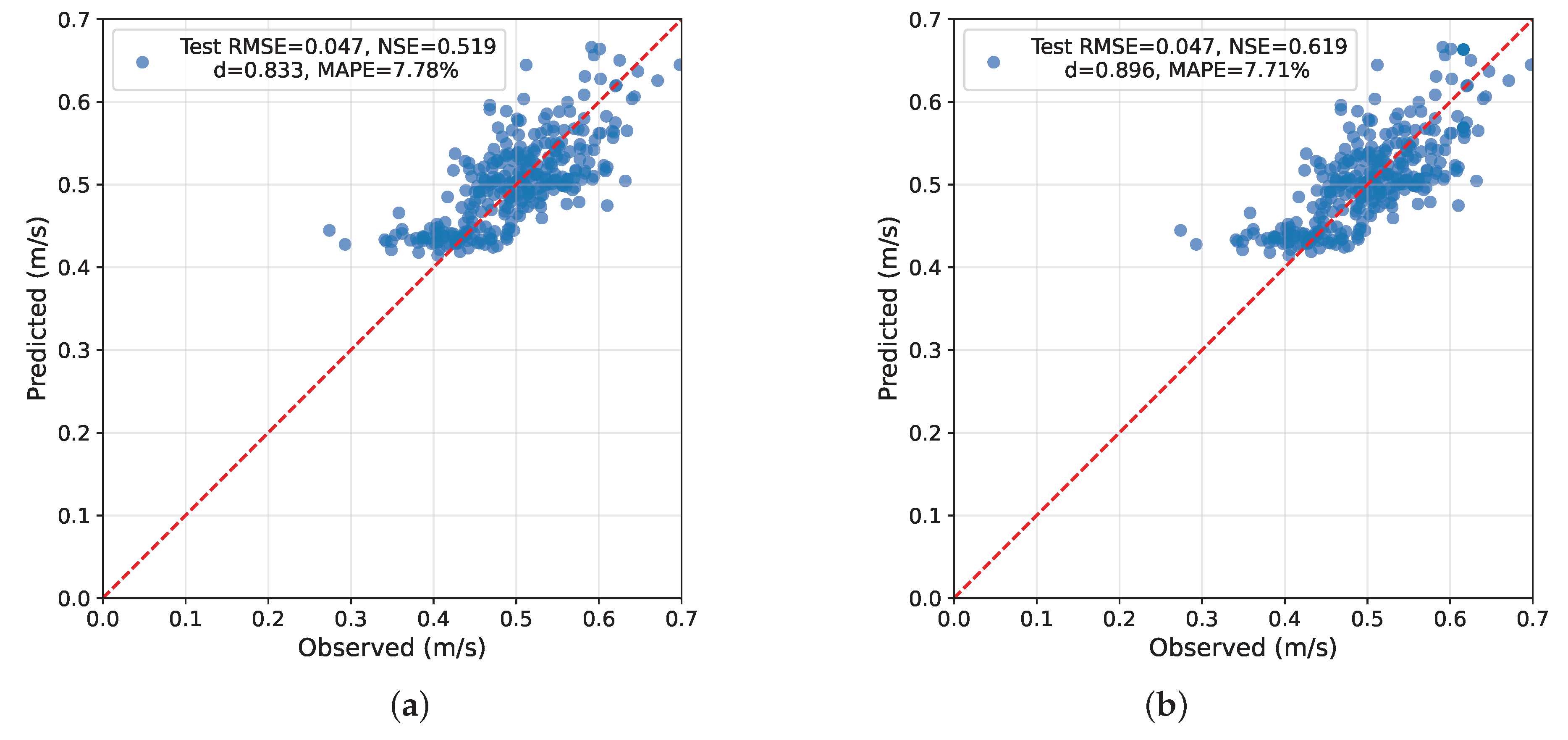
The second numerical example, termed the “all shift” scenario, uses the same base dataset as the previous section. As shown in Figure 2(a), the initial prediction–observation relationship yields the m/s and the , identical to the values in the earlier case. In this demonstration, the “all shift” algorithm appends an equal-sized block Z whose observations are tightly clustered around a shifted mean (mean shift only, negligible internal spread). This modification shifts the pooled mean and increases the total sum of squares (SST) through the between-mean term without introducing visible patterns; in our example, the absolute errors—and thus the RMSE—remain unchanged, whereas the NSE rises by exactly . The added points are subtle and visually indistinguishable, demonstrating that a controlled mean shift, rather than additional spread, can inflate the NSE without altering absolute prediction errors.
Figure 2(b) shows the resulting scatterplot after the algorithmic adjustment, with the m/s and the . Unlike the previous example, the added data are visually indistinguishable from the original points. This subtlety highlights the strength of the algorithm, as it can effectively enhance the NSE without introducing clearly visible artificial patterns. In practical situations, one could achieve similar results by carefully reweighting or selectively including specific observations. This example thus demonstrates that apparent performance improvements in the NSE can occur without genuine error reduction, emphasizing the need for caution when interpreting the NSE-based comparisons across datasets or models.
7. Conclusions
This study examined the relationship between the NSE and the RMSE across three evaluation scenarios. The key findings can be summarized as follows:
- 1.
- When models are evaluated on the same test dataset (Cases I and II), the rankings by the RMSE and the NSE are always consistent. A lower RMSE necessarily implies a higher NSE, and no contradictory outcomes are possible.
- 2.
-
When models are evaluated on unequal test datasets (Case III), contradictions may arise. In this setting, it is possible for one model to have a lower RMSE but simultaneously a lower NSE. The necessary and sufficient condition for this outcome, assuming that , is that the total variance of the expanded dataset more than doubles that of the original dataset, i.e.,This situation may occur if the new data block has very large variability, a substantial mean shift, or both.
- 3.
- A strengthened bound was derived showing that, for a targeted increase of in the NSE, one requireswhich guarantees that the combined RMSE is also larger than the original RMSE. This result generalizes the rule: when , the strengthened bound reduces exactly to . The implication is that an inferior model, already worse in the RMSE, can nevertheless appear superior under the NSE once the test dataset is artificially expanded. In other words, the model remains less accurate in absolute terms yet appears better in relative efficiency, exposing a structural vulnerability of the NSE.
In summary, the analysis demonstrates that the RMSE and the NSE provide fully consistent guidance when applied to a common test dataset, but contradictions emerge once models are compared across different evaluation bases. The inequalities derived here formalize the exact conditions under which such paradoxes occur, clarifying the mechanisms that drive apparent improvements in the NSE despite deteriorating the RMSE. For hydrological and machine learning applications, this emphasizes the critical importance of consistent evaluation datasets and cautions against overinterpreting the NSE values in cross-dataset comparisons, where a model may seem improved by the NSE even though its RMSE—and thus its absolute accuracy—is worse. By making these conditions explicit, the study contributes a rigorous theoretical foundation for interpreting efficiency metrics and highlights the need for transparency in evaluation design.
Supplementary Materials
The following supporting information can be downloaded at the website of this paper posted on Preprints.org.
Author Contributions
Conceptualization, methodology, software, validation, formal analysis, investigation, resources, data curation, writing—original draft preparation, writing—review and editing, visualization, supervision, project administration, and funding acquisition, W.C. The author has read and agreed to the published version of the manuscript.
Funding
This study was partially supported by the National Science and Technology Council (Taiwan) under Research Project Grant Numbers NSTC 114-2121-M-027-001, NSTC 114-2637-8-027-014, and NSTC 113-2121-M-008-004.
Institutional Review Board Statement
Not applicable.
Informed Consent Statement
Not applicable.
Data Availability Statement
No new data were created in this study. A Supplementary Document entitled “Supplementary Derivations for `On the Mathematical Relationship between RMSE and NSE across Evaluation Scenarios’ ” is provided, which contains detailed mathematical derivations and proofs supporting the equations and propositions discussed in the main text.
Acknowledgments
During the preparation of this manuscript, the author used ChatGPT 5 (OpenAI) for assistance in editing and polishing the writing. The author has reviewed and edited the output and takes full responsibility for the content of this publication. In addition, the entire manuscript has been professionally proofread by a native English speaker holding a Ph.D. degree to ensure grammatical accuracy and clarity.
Conflicts of Interest
The author declares no conflicts of interest.
References
- Nash, J.E.; Sutcliffe, J.V. River Flow Forecasting through Conceptual Models Part I—A Discussion of Principles. J. Hydrol. 1970, 10, 282–290. [Google Scholar] [CrossRef]
- Moriasi, D.N.; Arnold, J.G.; Van Liew, M.W.; Bingner, R.L.; Harmel, R.D.; Veith, T.L. Model evaluation guidelines for systematic quantification of accuracy in watershed simulations. Transactions of the ASABE 2007, 50, 885–900. [Google Scholar] [CrossRef]
- Amjad, N.; Ismail, M.; Ali, Z. Advancing future drought characterization: A two-phase Bayesian model averaging approach for GCM ensemble calibration. Applied Geomatics 2026, 18, 1–22. [Google Scholar] [CrossRef]
- Sung, J.; Jang, S.; Kim, T.; Kang, B. ConvLSTM-Based Surrogate Modeling for Flood Inflow Prediction at Namgang Dam. J. Hydrol. Eng. 2026, 31, 04025056. [Google Scholar] [CrossRef]
- Chen, H.; Song, X.; Xu, N.; Xu, C. Improving the Accuracy of Flood Forecasting Based on Deep Learning Models and Error Correction Methods: A Case Study of the Dapoling Watershed of the Huaihe River Basin, China. J. Hydrol. Eng. 2026, 31, 05025017. [Google Scholar] [CrossRef]
- Prajith, V.; Rahman, S.; Narasimha, K.; Gokul, T.S.; Pillai, A.N.; Das, N.V.; Ihjas, K. Modeling Infiltration Behavior to Assess the Reliability of Surface Flow Generation in Forested and Deforested Watersheds. J. Hydrol. Eng. 2026, 31, 04025046. [Google Scholar] [CrossRef]
- Niedzielski, T.; Ojrzyńska, H.; Miziński, B.; Kryza, M.; Spallek, W. Relationship between skills of multimodel hydrologic ensemble predictions and atmospheric circulation patterns: A case study from the Nysa Kłodzka river basin (SW Poland). Acta Geophys. 2025, 74, 25. [Google Scholar] [CrossRef]
- Wang, Z.; Ding, C.; Xu, N.; Wang, W.; Zhang, X. Interpretable Deep Learning Hybrid Streamflow Prediction Modeling Based on Multi-source Data Fusion. Environ. Model. Softw. 2025, 106796. [Google Scholar] [CrossRef]
- Lee, B.; Jeong, H.; Lee, Y.; McCarty, G.W.; Zhang, X.; Lee, S. Enhancement of hydrologic model optimization with single-step reinforcement learning. J. Hydrol. 2025, 134595. [Google Scholar] [CrossRef]
- Wang, W.-C.; Zhang, H.-Y.; Li, Z.; Ren, H.-Z. The CCVCLSA Model: A Novel Approach to Medium- and Long-Term Runoff Prediction Integrating Multiple Techniques. Results Eng. 2025, 108643. [Google Scholar] [CrossRef]
- Guo, J.; Jan, C.-D.; Guo, B. Modeling Rainfall Hyetographs from Cloud Droplet Size Distribution: A Similarity-Based Approach for Flood Nowcasting. J. Hydrol. Eng. 2026, 31, 04025053. [Google Scholar] [CrossRef]
- Diykh, M.; Ali, M.; Farooque, A.A.; Aldhafeeri, A.A.; Jamei, M.; Labban, A. A robust artificial intelligence informed over complete rational dilation wavelet transform technique coupled with deep learning for long-term rainfall prediction. Eng. Appl. Artif. Intell. 2026, 165, 113426. [Google Scholar] [CrossRef]
- El Bilali, A.; El Khalki, E.M.; Ait Naceur, K.; Jaffar, O.; El Ouafi, S.; Hadri, A. A hybrid approach for groundwater level prediction: Integrating water balance model state variables and machine learning algorithms. Environ. Earth Sci. 2026, 85, 10. [Google Scholar] [CrossRef]
- Huang, J.; Yang, Z.; Li, M.; Wu, Y.; Shiau, J. Experimental study of active earth pressure on 3D-printed flexible retaining walls. Measurement 2025, 119364. [Google Scholar] [CrossRef]
- Liu, C.-Y.; Ku, C.-Y.; Wu, T.-Y.; Chiu, Y.-J.; Chang, C.-W. Liquefaction susceptibility mapping using artificial neural network for offshore wind farms in Taiwan. Eng. Geol. 2025, 351, 108013. [Google Scholar] [CrossRef]
- Zhang, Q.; Miao, C.; Gou, J.; Zheng, H. Spatiotemporal characteristics and forecasting of short-term meteorological drought in China. J. Hydrol. 2023, 624, 129924. [Google Scholar] [CrossRef]
- Hu, J.; Miao, C.; Zhang, X.; Kong, D. Retrieval of suspended sediment concentrations using remote sensing and machine learning methods: A case study of the lower Yellow River. J. Hydrol. 2023, 627, 130369. [Google Scholar] [CrossRef]
- Sahour, H.; Gholami, V.; Vazifedan, M.; Saeedi, S. Machine learning applications for water-induced soil erosion modeling and mapping. Soil Tillage Res. 2021, 211, 105032. [Google Scholar] [CrossRef]
- Chen, W.; Nguyen, K.A.; Lin, B.-S. Rethinking Evaluation Metrics in Hydrological Deep Learning: Insights from Torrent Flow Velocity Prediction. Sustainability 2025, 17, 8658. [Google Scholar] [CrossRef]
- Chen, W.; Nguyen, K.A.; Lin, B.-S. Deep Learning and Optical Flow for River Velocity Estimation: Insights from a Field Case Study. Sustainability 2025, 17, 8181. [Google Scholar] [CrossRef]
- Schaefli, B.; Gupta, H.V. Do Nash values have value? Hydrol. Process. 2007, 21, 2075–2080. [Google Scholar] [CrossRef]
- Clark, M.P.; Vogel, R.M.; Lamontagne, J.R.; Mizukami, N.; Knoben, W.J.M.; Tang, G.; Papalexiou, S.M. The abuse of popular performance metrics in hydrologic modeling. Water Resour. Res. 2021, 57, e2020WR029001. [Google Scholar] [CrossRef]
- Gupta, H.V.; Kling, H.; Yilmaz, K.K.; Martinez, G.F. Decomposition of the mean squared error and NSE performance criteria: Implications for improving hydrological modelling. J. Hydrol. 2009, 377, 80–91. [Google Scholar] [CrossRef]
- Williams, G.P. Friends Don’t Let Friends Use Nash–Sutcliffe Efficiency (NSE) or KGE for Hydrologic Model Accuracy Evaluation: A Rant with Data and Suggestions for Better Practice. Environ. Model. Softw. 2025, 106, 106665. [Google Scholar] [CrossRef]
- Melsen, L.A.; Puy, A.; Torfs, P.J.J.F.; Saltelli, A. The Rise of the Nash–Sutcliffe Efficiency in Hydrology. Hydrol. Sci. J. 2025, 1–12. [Google Scholar] [CrossRef]
- Onyutha, C. Pros and Cons of Various Efficiency Criteria for Hydrological Model Performance Evaluation. Proc. IAHS 2024, 385, 181–187. [Google Scholar] [CrossRef]
- Lamontagne, J.R.; Barber, C.A.; Vogel, R.M. Improved Estimators of Model Performance Efficiency for Skewed Hydrologic Data. Water Resour. Res. 2020, 56, e2020WR027101. [Google Scholar] [CrossRef]
- Willmott, C.J.; Matsuura, K. Advantages of the mean absolute error (MAE) over the root mean square error (RMSE) in assessing average model performance. Climate Research 2005, 30, 79–82. [Google Scholar] [CrossRef]
- Willmott, C.J.; Matsuura, K.; Robeson, S.M. Ambiguities inherent in sums-of-squares-based error statistics. Atmospheric Environment 2009, 43, 749–752. [Google Scholar] [CrossRef]
- Chai, T.; Draxler, R.R. Root Mean Square Error (RMSE) or Mean Absolute Error (MAE)?—Arguments Against Avoiding RMSE in the Literature. Geosci. Model Dev. 2014, 7, 1247–1250. [Google Scholar] [CrossRef]
Figure 1.
Numerical demonstration of the “all spread” scenario using real data from the Yufeng No. 2 stream. (a) Before applying the algorithm (, ); (b) After applying the algorithm (, ). Increasing the variance of the observed dataset through the spread operation raises the NSE by while keeping the RMSE constant.
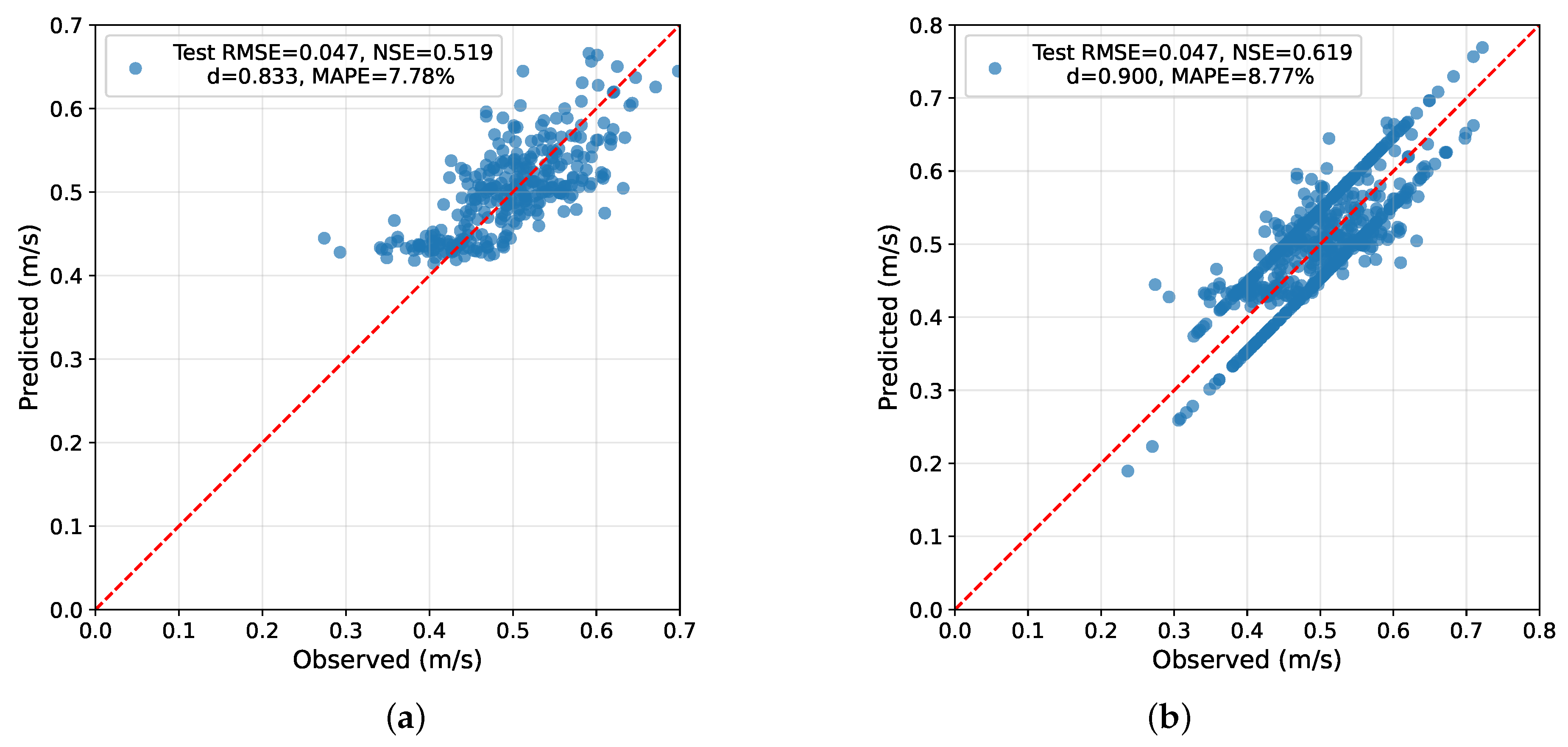
Figure 2.
Numerical demonstration of the “all shift” scenario using real data from the Yufeng No. 2 stream. (a) Before applying the algorithm (, ); (b) After applying the algorithm (, ). The shift operation adds a block of data with a shifted mean and minimal spread, increasing the NSE by while keeping the RMSE unchanged and the added points nearly invisible.
Disclaimer/Publisher’s Note: The statements, opinions and data contained in all publications are solely those of the individual author(s) and contributor(s) and not of MDPI and/or the editor(s). MDPI and/or the editor(s) disclaim responsibility for any injury to people or property resulting from any ideas, methods, instructions or products referred to in the content. |
© 2026 by the authors. Licensee MDPI, Basel, Switzerland. This article is an open access article distributed under the terms and conditions of the Creative Commons Attribution (CC BY) license (http://creativecommons.org/licenses/by/4.0/).
Copyright: This open access article is published under a Creative Commons CC BY 4.0 license, which permit the free download, distribution, and reuse, provided that the author and preprint are cited in any reuse.


