Submitted:
25 December 2024
Posted:
26 December 2024
You are already at the latest version
Abstract
The Nash–Sutcliffe efficiency remains the best metric of the appropriateness of a model, and reflects a culture developed in hydrology to test models against reality before using them. This metric is not without problems and alternative metrics have been proposed subsequently. Here the concept of knowable moments is exploited to provide robust metrics, that assess not only the second-order properties of the process of interest but also high-order moments which provide information for the entire distribution function of the process of interest. This information may be useful in hydrological tasks, as most hydrological processes are non-Gaussian. The proposed concepts are illustrated, also in analogy to existing ones, with a large-scale comparison of climatic model outputs for precipitation with reality for the last 84 years on hemispheric and continental scales.
Keywords:
Model efficiency
; Nash – Sutcliffe efficiency
; reality check
; bias
; explained variance
; unexplained variation
; knowable moments
All models are wrong but some are useful (George E. P. Box ) (Box, G. E. P. Robustness in the Strategy of Scientific Model Building. Robustness in Statistics 1979, 201–236. doi:10.1016/b978-0-12-438150-6.50018-2.).
1. Introduction
The aphorism in the epigram is very popular and expresses the fact that models are only approximations of reality. The first part of aphorism, “all models are wrong” is wrong per se in a rigorous epistemological context. The meaning it purports to express could perhaps be better formulated as “models differ from reality”. They differ not only in quantitative terms—e.g., when a real value is 6 units and a model predicts 5 units. Even if a model gives a value identical to the real one (e.g. 6 units), again it differs from reality conceptually as the model is a representation (usually mathematical, simplifying and approximate) of reality—not the physical reality per se [[1]]. The model differs from the system it represents even in the case that the latter is a hardware and/or software implementation of an algorithm [[2]]. In an era where confusion has prevailed over rigour, it is essential to clarify the conceptual difference, which makes a model not “wrong” or “right”—just conceptually different from reality.
The second part of the aphorism, “some [models] are useful” is not problematic and is the subject of this paper. The usefulness of a model is an issue that needs modelling per se. In other words, it needs to be quantified by metrics that describe how good a quantified approximation of reality is. This quantification is typically based on simulation results by the model and comparison with observations. The comparison typically uses statistical or stochastic concepts such as variances and correlation coefficients. This implies that we have to take an additional modelling step, i.e. to assume that both model simulation outputs, , and actual observations, , are further represented as stochastic variables (or even stochastic processes), (notice the notational convention to underline stochastic variables). This step may not be necessary if the model is deterministic, yet taking it allows using the advanced language and tools of stochastics, which facilitates modelling.
Standard statistical metrics of this type are the correlation coefficient, , between and , and its square, , known as the coefficient of determination. These however do not provide a holistic picture of the similarity between and as they do not reflect the similarity (or otherwise) of the marginal distribution. For example, and may have a large , suggesting good model performance, and simultaneously a large difference in their means, suggesting poor performance because of bias.
The most common metric of a holistic type has been the Nash–Sutcliffe efficiency (NSE). It was proposed by two famous hydrologists, Nash and Sutcliffe (1970) [[3]] in a study that for a long time has been the most cited hydrological paper [[4]] (currently about 28 000 citations in Google Scholar and more than 18 000 in Scopus). Its use has been common beyond hydrology, such as in geophysics, earth sciences, atmospheric sciences, environmental sciences, statistics, engineering, data science and computational intelligence [e.g. [5]-,[6],[7],[8],[9],[10],[11],[12],[13],[14],[15],[16]]. As noted by O’Connell et al. [[17]], the discipline of hydrology has commonly been an “importer” of ideas, techniques and theories developed in other scientific disciplines. A rare exception is Hurst’s work [[18]], which was “exported” to many areas of science and technology. The model performance metric proposed by Nash and Sutcliffe (NSE) is another rare exception of “exportation”.
A different metric that has recently attracted wide attention in hydrology and beyond is the Kling–Gupta efficiency (KGE) proposed by the hydrologists Kling and Gupta [[19],[20]]. Both metrics, NSE and KGE, are expressed in terms of the first- and second-order classical moments of the variables or their difference, i.e., the error . Both are dimensionless and have an upper bound, the number 1, which corresponds to perfect agreement of simulated with observed values. However, they have differences. NSE has a conceptual and rigorous definition based on the expectation of the squared error. KGE is a rather arbitrary expression, heuristically combining three indices of agreement. These also appear in NSE, if it is decomposed using stochastic algebra. It is useful that the KGE metric distinguishes the three separate indicators of agreement, but it is doubtful if their combination in one metric is useful.
Both NSE and KGE provide useful information for processes that are Gaussian or close to Gaussian, but, as will be shown in the analyses that follow, fail to perform in processes with behaviour far different from Gaussian. Therefore, we need some metrics that can provide useful information for the latter case. In addition, in non-Gaussian processes, we usually need information about the behaviour at the distribution tails. This can hardly be extracted from second-order statistical properties. On the other hand, high-order moments are unknowable if the information is extracted from data [[21]-,[22],[23],[24],[25]]. Yet, the new concept of knowable moments or K-moments [23-26] can replace the classical second-order moments, on the one hand, and extend the definition of metrics for high orders, on the other hand. This is attempted in this study, after re-examining the NSE and KGE metrics, which are based on classical moments, and locating their strengths and weaknesses (Section 2). An alternative framework based on K-moments is proposed and some synthetic examples are used to illustrate the properties of both the existing and the proposed frameworks (Section 3). In addition, an application with real-world processes, namely the precipitation process, is presented, where the real system is assumed to be described by reanalysis data for precipitation, while the models are assumed to be some popular climate models (Section 4).
2. Revisiting the Existing Framework
2.1. Nash – Sutcliffe Efficiency
The error between the simulated and actual processes is defined as
Based on this, the Nash – Sutcliffe efficiency is defined as
The error can be decomposed as
with . Hence, the NSE can be decomposed as
where EV and RV are the explained variance and the relative bias, respectively:
Alternatively, in the decomposition, we can substitute the statistics of for those of and find
Hence:
It follows directly that, when, the metrics are maximized for:
and their maximum value is
Notably, the maximum value is not achieved when . Rather, the value that corresponds to the latter case is
2.1. Kling–Gupta Efficiency and Its Relationship with the Nash – Sutcliffe Efficiency
The Kling–Gupta efficiency is defined as
The definition is heuristic and thus KGE does not represent a formal statistic. The last term is pathological as it is often the case that (e.g. when departures from the mean, known as “anomalies”, are modelled), in which KGE becomes . If we exclude the pathological last term, KGE becomes equivalent, but not equal, to EV in the sense that both express second-order properties.
The maximum value of KGE is achieved for , and is
For , after algebraic operations, we find that KGE and EV are related by
In the limiting case that (and ), we find
Equations (13) and (14) are illustrated in Figure 1, where it can be seen that (a) when the explained variance EV = NSE is high, say > 0.5, the value of KGE is smaller than EV; (b) when EV = NSE is zero, the value of KGE can be as high as 0.5 (for ; (c) when the EV is negative, the KGE value is less negative; (d) in general, KGE tends to decrease, in absolute value, the effectiveness metric that is provided by the EV = NSE; (e) this is further verified from the curve corresponding to which has a slope of 1/2, instead of 1. In brief, KGE is a less sensitive metric than NSE.
All in all, the heuristic character, the smaller sensitivity and the problematic division by the mean, which can be zero, do not favour the use of KGE and thus it will not be used further in the rest of this paper. A substitute with some mathematical meaning, namely the absolute error efficiency, AEE (rather than the squared error in NSE), is the following, computed in Appendix A:
Notice that the quantity is not squared, as is in KGE; actually, squaring is not necessary from a mathematical point of view as it is always nonnegative. Assuming that , the resulting AEE is , which takes a zero value for . Like in the NSE case, when, is maximized not when , but when satisfies equation (8).
3. Proposed Framework
3.1. A Summary of K-Moments
The methodologies discussed in Section 2 are based on first and second-order distributional properties, while the framework of classical moments cannot serve estimation of higher-order moments [22,23,26]. However, the concept of knowable moments or K-moments [23-26] can work for high -order moments.
The K-moments are defined as follows. We consider a sample of a stochastic variable , i.e., a number of independent copies of the stochastic variable , i.e., . If we arrange the variables in ascending order, the ith smallest, denoted as is termed the ith order statistic. The largest (pth) order statistic is:
and the smallest (first) is
Now we define the upper knowable moment (K-moment) of order p as the expectation of the largest of the p variables :
where denotes expectation, and the lower knowable moment (K-moment) of order p as the expectation of the smallest of the p variables :
An important property, directly resulting from their definition, is that the K-moments are ordered as follows:
These moments are noncentral and we can also define central moments as
As shown in [26] (chapter 6), for a stochastic variable of continuous type, the upper K-moment of order p of , is theoretically calculated as:
Likewise, the lower K-moment of order p is theoretically calculated as:
In these equations, is the distribution function of , is its tail function and is its probability density function. For discrete type variables as well as for generalizations of K-moments, the interested reader is referred to [25,26].
The unbiased estimator of the upper K-moment from a sample is
and that of the lower K-moment is,
where
where is the gamma function. For integer moment order and this simplifies to
Based on the K-moments, we define the location (or central tendency) parameter of order , , the dispersion parameter of order , , and the dispersion ratio of order , , as:
where . The least-order meaningful values thereof are:
Note that when
Also, as [26], we have .
3.2. K-moments Based Metrics of Efficiency
A perfect model will have all central tendency and dispersion parameters equal to zero: for any . A good model will have nonzero values but not large. Based on the dispersion parameters, , we can define quantities, analogous to the explained variance. We define the K-unexplained variation of order and its difference from 1, the K-explained variation of order as:
Their least-order meaningful values are
The minimum and maximum possible values are respectively and , and correspond to . For a model that equates any with the mean of , for any , and . Models worse than that have higher than 1 and negative values of .
For a normal distribution, and hence the K-moments based metrics are related to the classical explained variance by
Reminding that for , (see Figure 1), we notice the identity of and (as functions of EV) for this case and further observe that Equation (32) holds for any for normal distribution, while that for KGE only holds for .
The bias is a separate characteristic and it would be better treated based on a different statistic. The ratio is an appropriate metric for it. Alternatively—and in an analogous manner to —we can define the K-bias of order p as
with a special case for
It appears more natural for the two quantities describing dispersion and bias to be thought of as small as possible in order for a model to be regarded as good. To fulfil this desideratum, the metrics of choice would be the and . However, as the aim of this paper is to provide metrics with behaviour similar to the existing ones, in what follows we use rather than the more natural . In the case that the unexplained variation and bias are to be combined, a relevant expression, called the K-moment-based absolute error efficiency and derived in Appendix A, is:
3.2. Possible Transformations of Data
Figure 2 (upper) compares two synthetic time series consisting of 1000 data values, an original and a simulated . These synthetic series were constructed as follows. First a series was generated from the Hurst-Kolmogorov model with Hurst parameter 0.95 and normal distribution N(0,1). Then the series was smoothed by a linear filter with a triangular shape, with a peak value of 1 and zero values at times 10 and 20 time steps before and after the time of the peak, respectively, thus producing a series . Subsequently, a series was generated by adding to a series again generated from the Hurst-Kolmogorov model with Hurst parameter 0.95 and normal distribution N(0,), where is the standard deviation of . Finally, the two latter series were exponentiated, , with , and taken as original and simulated series after rounding to one decimal point. Both and exhibit long-range dependence and are lognormally distributed. The former is rough, due to the component , while the latter is smooth.
From the visual depiction of Figure 2 (upper) it turns out that the model performance is very poor. This is also reflected in all metrics shown in Table 1 (first row). However, the poor performance is mostly due to the log-normal distribution of , which yields frequent high peaks. The simulated series does not capture these peaks. If we take the logarithmic transformations of both and , then, as seen in Figure 2 (middle), there is some resemblance of the original and simulated series, which is also reflected in the metrics of Table 1 for the log-transformed series.
This fact suggests that if the series examined are not normally distributed, a transformation of the data may be necessary before assessing the suitability of the model through appropriate indices. The logarithmic transformation may not be appropriate for all cases and also has a problem, namely the fact that it diverges to minus infinity when the original value is zero. The latter problem was resolved in an ad hoc manner to calculate the values in Table 1, i.e. by mapping the zero values in and to the logarithm of 0.01 (one order of magnitude lower than the minimum value, which is 0.1).
A proper transformation that remedies these problems, by being general and avoiding ad hoc considerations, is the following [26] (section 2.10), which we denote as lambda (λ) transformation:
and likewise for . For low values of , including , this maps to itself, while for large it maps it to a linear function of . The parameter λ is assumed to be the same for both and . We can estimate it numerically by maximizing one of the model efficiency metrics.
Furthermore, for the simulated series, unless the model is physically based and its simulation results have some physical meaning, we may give it some more degrees of freedom by the additional parameters α and β using the transformation
with default values . Again, these are obtained by optimization together with the optimization of , noting that applies to both and , but α and β apply to only. Table 1 gives the optimized values of for the default values of α and β, as well as the optimized values of all three parameters, and the resulting optimal metrics of model efficiency. Figure 2 (lower) shows the transformed time series and , where a good agreement between the two is seen, in contrast to the upper panel of the same figure.
The metrics optimized for the two λ-transformed series of Table 1 are the KEV₂ when the default default values are used and the KAEE otherwise. These are not the only options as high-order metrics could also have been chosen to be optimized. The higher-order metrics when the KEV₂ is optimized are shown in Figure 3 (left), also in comparison to those of the untransformed series. As seen in the figure, the performance deteriorates with the increase of the moment order. On the other hand, Figure 3 (right) shows that the performance, in terms of the KEV₂ metric, improves when the time scale increases.
Figure 3 does not give any information about the model bias. This is provided in Figure 4 in terms of both the ratio and the K-bias. As seen in the graphs, both indices practically provide the same information and there is no substantial variation of the bias metrics with order p. However, the λ transformation reduces the bias of the original series substantially.
4. Real World Case Study
To present a large-scale case study of hydrological interest, we use the results of climate models for precipitation, which have been very popular and widely used in so-called climate impact studies, but without proper testing whether they are useful or not. The climate models (also known as global circulation models—GCM) used belong to the last-generation Coupled Model Intercomparison Project (CMIP6) and their outputs for precipitation were retrieved from the Koninklijk Nederlands Meteorologisch Instituut (KNMI) Climate Explorer [[26],[27]]. The outputs from the 37 models listed in Table 2 were available on a monthly scale and were aggregated to annual and over-annual scales.
As a time series representing reality, the gridded data of the ERA5 reanalysis were used [[28]]. This is the fifth-generation atmospheric reanalysis of the European Centre for Medium Range Weather Forecasts (ECMWF), where the name ERA refers to ECMWF ReAnalysis. ERA5 has been produced as an operational service and its fields compare well with the ECMWF operational analyses. It combines vast amounts of historical observations into global estimates using advanced modelling and data assimilation systems. The data are available for the period 1940-now at a spatial resolution of 0.5° globally and were retrieved using the Web-based Reanalyses Intercomparison Tools (WRIT) [[29]] made available by the USA National Oceanic and Atmospheric Administration (NOAA). The comparisons of models and reality, represented by ERA5, were made for the period 1940-2023 (84 years), separately for the North Hemisphere (NH) and the South Hemisphere (SH). A visual comparison of the time series is presented using spaghetti graphs in Figure 5 on the annual scale and Figure 6 on 8-year scale. The latter was selected as the maximum climatic scale that allows 10 data points, so that statistics can be estimated.
A prominent characteristic seen in the spaghetti graphs is the large bias of models, which is mostly negative for NH and mostly positive for SH. Different models have largely different bias. The large bias in precipitation certainly reflects inappropriate modelling of the physical processes related to the hydrological cycle, starting with latent heat and evaporation.
Nonetheless, Figure 7 shows that on a hemispheric basis there is correlation between models and reality, with an average of 0.31 for NH and 0.11 for SH. An interesting property is that each model’s precipitation at NH is negatively correlated to that of the same model for the SH, with an average correlation of –0.61. This model property, however, does not correspond to reality: if this correlation is estimated from the ERA5 data it is practically zero (–0.03).
These correlations are not enough to suggest usefulness of the models in terms of the explained variance. As seen in Figure 8, both classical and K-explained variance are mostly negative on the annual scale. Yet, positive values appear on the 8-year scale. However, if we also consider the bias, which is shown in Figure 9, the total efficiency metrics, NSE and KAEE take highly negative values, which prohibit any usefulness of the climate models for hydrological purposes.
A most relevant question is whether or not some of the models have relatively good performance in general. To study this question we first assess which of the models have the best performance, in a Pareto optimality sense, for both hemispheres. To this aim, we plot in Figure 10 the cross-performance of the GCMs at both hemispheres, in terms of the K-explained variation, KEV₂, on annual and 8-year time scales. On the annual scale, the models show mostly negative explained variation, that is, poor performance. On the 8-year scale, the performance is improved. The two models with the best performance appear to be the CMCC-CM2-SR5 and FGOALS-f3-L.
The change of the performance with moment order and time scale for model CMCC-CM2-SR5 is shown in Figure 11, where it is seen that for small time scales the performance is not good in none of the hemispheres. Figure 12 shows that the performance at the annual scale can be slightly improved by applying the transformation of Equation (37), but this is accompanied by a worsening of the performance at large time scales. Interestingly, the improvement at the annual scale is due to the linear part of the transformation, namely on the parameter , and not due to the logarithmic part.
The next step is to choose an area smaller than an entire hemisphere and assess the performance of the two “best performing” models in this area. Given that ERA5 is developed in Europe and hence expected to be more accurate in this area, we chose a spherical rectangle that contains Europe, namely that defined by the coordinates 11° W, 40° E, 34° N, 71° N. The time series of the two models in question, integrated over this area, are shown in Figure 13, in comparison with the ERA5 time series. The visual comparison is not encouraging in terms of the agreement of models with reality.
Even without considering the bias, which is substantial, i.e., by only considering the explained variation, the results are rather disappointing, with not exceeding 0.1 at any scale .
5. Discussion and Conclusions
The classical Nash–Sutcliffe efficiency appears to be a good metric of the appropriateness of a model. Yet its fusion of two different characteristics, the explained variance and the bias, is not always an advantage. The bias could be a very important characteristic if a model is physically based and the bias reflects a violation of a physical law (e.g. conservation of mass of energy). In such cases, a large bias would suffice to reject a model, even if it captures the variation patterns.
In other cases, in which the model is of conceptual mathematical, rather than physical, type, the bias can be easily removed by a shift of the origin. In such cases, a nonlinear transformation of the observed and modelled series, accompanied by a linear transformation of the simulated series (Equations (36) – (37)), can potentially improve the agreement between the model and reality. It is suggested that in such cases, the quantified assessment of model usefulness be based on the metrics of the transformed series.
The typical metrics that are currently used to assess model performance are based on classical statistics up to second order. This is not a problem when the processes are Gaussian, but most hydrological processes are non-Gaussian. The concept of knowable moments (K-moments) offers the basis to extend the performance metrics to high orders, up to the sample size. The two metrics proposed, the K-unexplained variation, , and the K-bias, , both based on K-moments of the model error, provide ideal means to assess the agreement of models with reality; the closer to zero they are, the better the agreement. The lowest order on which they are evaluated is , which represents second-order properties, but also using higher orders gives useful information on the agreement of the entire distribution functions.
The real-world application presented is a large-scale comparison of climatic model outputs for precipitation with reality for the last 84 years. It turns out that the precipitation simulated by the climate model does not agree with reality on the annual scale but there is some improvement on larger time scales at a hemispheric basis. However, when the areal scale is decreased from hemispheric to continental, i.e. when Europe is examined, the model performance is poor even at large time scales. Therefore the usefulness of climate model results for hydrological purposes is doubtful.
Supplementary Materials
N/A.
Author Contributions
N/A.
Funding
This research received no external funding but was conducted out of scientific curiosity.
Data Availability Statement
No new data were created in this study. The data sets used were retrieved from the sources described in detail in the text.
Acknowledgments
N/A.
Conflicts of Interest
The author declares no conflicts of interest.
Appendix A
To find a holistic metric of efficiency based on K-moments, we assume normal distribution of and —and hence of — and we find the expectation of the absolute error. which, after algebraic calculations, turns out to be:
When we estimate from the mean value , so that the expected estimation error be zero and have standard deviation , then the absolute error has expectation:
Hence we may formulate an efficiency metric based on the absolute error as
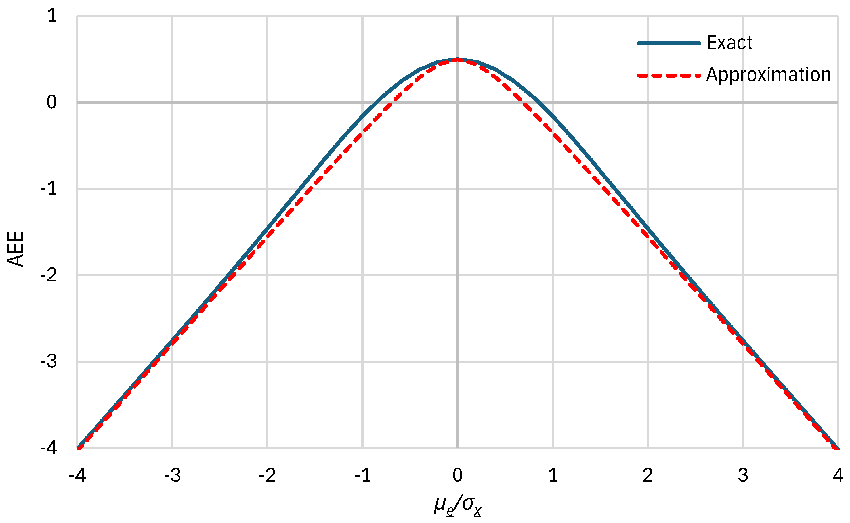
As the expression in the big parentheses tends to and its derivative with respect to tends to 0. As the same expression tends to . The same behaviour is shared by the following approximation
This was devised after noting that the square of the absolute error can be approximated by its second-order Taylor expression, i.e., . Figure A1 shows that the approximation is meaningful. We can also express AEE using the joint distribution characteristics of and instead of those of and . In this case, after algebraic operations, we obtain Equation (15). Furthermore, we can substitute K-moments for classical moments, noting that and for the normal distribution (Koutsoyiannis, 2023, Table 6.3).
In this case we obtain:
which can be written in the form of Equation (35).
Figure A1.
Graphical comparison of the exact relationship of the absolute error efficiency for a normal distribution, as given by Equation (A3), with its approximation given by Equation (A4).
Figure A1.
Graphical comparison of the exact relationship of the absolute error efficiency for a normal distribution, as given by Equation (A3), with its approximation given by Equation (A4).
References
- Koutsoyiannis, D.; Montanari, A. Negligent killing of scientific concepts: the stationarity case. Hydrological Sciences Journal 2015, 60, 1174–1183. [Google Scholar] [CrossRef]
- Kurshan, R. Computer-Aided Verification of Coordinating Processes: The Automata-Theoretic Approach, ISBN: 0-691-03436-2 Princeton Univ. Press, Princeton, New Jersey, USA, 1994.
- Nash, J.E.; Sutcliffe, J.V. River flow forecasting through conceptual models, part I—A discussion of principles. Journal of hydrology 1970, 10, 282–290. [Google Scholar] [CrossRef]
- Koutsoyiannis, D.; Kundzewicz, Z.W. Editorial - Quantifying the impact of hydrological studies, Hydrological Sciences Journal 2007, 52, 3–17.
- Willmott, C.J.; Ackleson, S.G.; Davis, R.E.; Feddema, J.J.; Klink, K.M.; Legates, D.R.; O'Donnell, J.; Rowe, C.M. Statistics for the evaluation and comparison of models. Journal of Geophysical Research: Oceans 1985, 90, 8995–9005. [Google Scholar] [CrossRef]
- Willmott, C.J.; Robeson, S.M.; Matsuura, K. A refined index of model performance. International Journal of Climatology 2012, 32, 2088–2094. [Google Scholar] [CrossRef]
- Bennett, N.D.; Croke, B.F.; Guariso, G.; Guillaume, J.H.; Hamilton, S.H.; Jakeman, A.J.; Marsili-Libelli, S.; Newham, L.T.; Norton, J.P.; Perrin, C.; Pierce, S.A. Characterising performance of environmental models. Environmental Modelling & Software, 2013; 40, 1–20. [Google Scholar]
- Huang, C.; Chen, Y.; Zhang, S.; Wu, J. Detecting, extracting, and monitoring surface water from space using optical sensors: A review. Reviews of Geophysics 2018, 56, 333–360. [Google Scholar] [CrossRef]
- Reichstein, M.; Camps-Valls, G.; Stevens, B.; Jung, M.; Denzler, J.; Carvalhais, N.; Prabhat, F. Deep learning and process understanding for data-driven Earth system science. Nature 2019, 566, 195–204. [Google Scholar] [CrossRef] [PubMed]
- Zurell, D.; Franklin, J.; König, C.; Bouchet, P.J.; Dormann, C.F.; Elith, J.; Fandos, G.; Feng, X.; Guillera-Arroita, G.; Guisan, A.; Lahoz-Monfort, J.J. A standard protocol for reporting species distribution models. Ecography 2020, 43, 1261–1277. [Google Scholar] [CrossRef]
- Peng, S.; Ding, Y.; Liu, W.; Li, Z. 1 km monthly temperature and precipitation dataset for China from 1901 to 2017. Earth System Science Data 2019, 11, 1931–1946. [Google Scholar] [CrossRef]
- Hassani, A.; Azapagic, A.; Shokri, N. Predicting long-term dynamics of soil salinity and sodicity on a global scale. Proceedings of the National Academy of Sciences 2020, 117, 33017–33027. [Google Scholar] [CrossRef] [PubMed]
- Hassani, A.; Azapagic, A.; Shokri, N. Global predictions of primary soil salinization under changing climate in the 21st century. Nature Communications 2021, 12, 6663. [Google Scholar] [CrossRef] [PubMed]
- Yaseen, Z.M. An insight into machine learning models era in simulating soil, water bodies and adsorption heavy metals: Review, challenges and solutions. Chemosphere 2021, 277, 130126. [Google Scholar] [CrossRef]
- Naser, M.Z.; Alavi, A.H. Error metrics and performance fitness indicators for artificial intelligence and machine learning in engineering and sciences. Architecture, Structures and Construction 2023, 3, 499–517. [Google Scholar] [CrossRef]
- Martinho, A.D.; Hippert, H.S.; Goliatt, L. Short-term streamflow modeling using data-intelligence evolutionary machine learning models. Scientific Reports 2023, 13, 13824. [Google Scholar] [CrossRef] [PubMed]
- O’Connell, P.E.; Koutsoyiannis, D.; Lins, H.F.; Markonis, Y.; Montanari, A.; Cohn, T.A. The scientific legacy of Harold Edwin Hurst (1880 – 1978), Hydrological Sciences Journal 2016, 61, 1571–1590. [CrossRef]
- Hurst, H.E. Long-Term Storage Capacity of Reservoirs. Trans. Am. Soc. Civ. Eng. 1951, 116, 770–799. [Google Scholar] [CrossRef]
- Gupta, H.V.; Kling, H. On typical range, sensitivity, and normalization of Mean Squared Error and Nash-Sutcliffe Efficiency type metrics. Water Resources Research 2011, 47. [Google Scholar] [CrossRef]
- Kling, H.; Fuchs, M.; Paulin, M. Runoff conditions in the upper Danube basin under an ensemble of climate change scenarios. Journal of Hydrology 2012, 2012. 424, 264–277. [Google Scholar] [CrossRef]
- Lombardo, F.; Volpi, E.; Koutsoyiannis, D.; Papalexiou, S.M. Just two moments! A cautionary note against use of high-order moments in multifractal models in hydrology. Hydrology and Earth System Sciences 2014, 18, 243–255. [Google Scholar] [CrossRef]
- Koutsoyiannis, D. Knowable moments for high-order stochastic characterization and modelling of hydrological processes, Hydrological Sciences Journal 2019, 64, 19–33. [CrossRef]
- Koutsoyiannis, D. Replacing histogram with smooth empirical probability density function estimated by K-moments, Sci 2022, 4, 50. [CrossRef]
- Koutsoyiannis, D. Knowable moments in stochastics: Knowing their advantages, Axioms 2023, 12, 590. [CrossRef]
- Koutsoyiannis, D. Stochastics of Hydroclimatic Extremes - A Cool Look at Risk, Edition 3, ISBN: 978-618-85370-0-2, 391 pages, Kallipos Open Academic Editions, Athens, 2023. [CrossRef]
- Trouet, V.; Van Oldenborgh, G.J. KNMI Climate Explorer: a web-based research tool for high-resolution paleoclimatology. Tree-Ring Research 2013, 69, 3–13. [Google Scholar] [CrossRef]
- The KNMI climate explorer. Available online: https://climexp.knmi.nl/start.cgi (accessed on 19 August 2024).
- ERA5: data documentation - Copernicus Knowledge Base - ECMWF Confluence Wiki. Available online: https://confluence.ecmwf.int/display/CKB/ERA5%3A+data+documentation (accessed on 25 March 2023).
- Web-based Reanalyses Intercomparison Tools, Available online:. Available online: https://psl.noaa.gov/data/atmoswrit/timeseries/index.html (accessed on 19 August 2024).
Figure 1.
Relationship of KGE and NSE for and the indicated values of LC stands for the limiting curve corresponding to , for which . Nb., for KGE is (precisely when or somewhat smaller for different EV values).
Figure 1.
Relationship of KGE and NSE for and the indicated values of LC stands for the limiting curve corresponding to , for which . Nb., for KGE is (precisely when or somewhat smaller for different EV values).
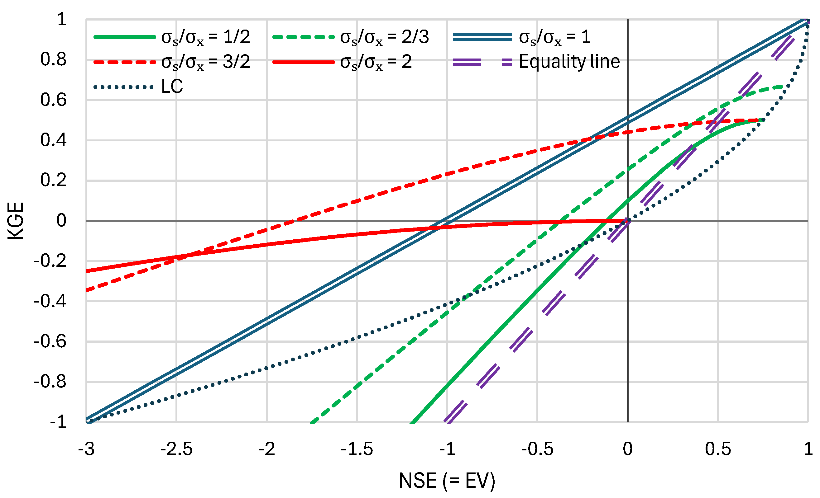
Figure 2.
An example illustrating a case in which the poor performance of a model improves substantially after transformation of the variables: (upper) original series on a decimal plot; (middle), original series on a logarithmic plot; (lower) λ-transformed series with parameters shown in Table 1 (last row).
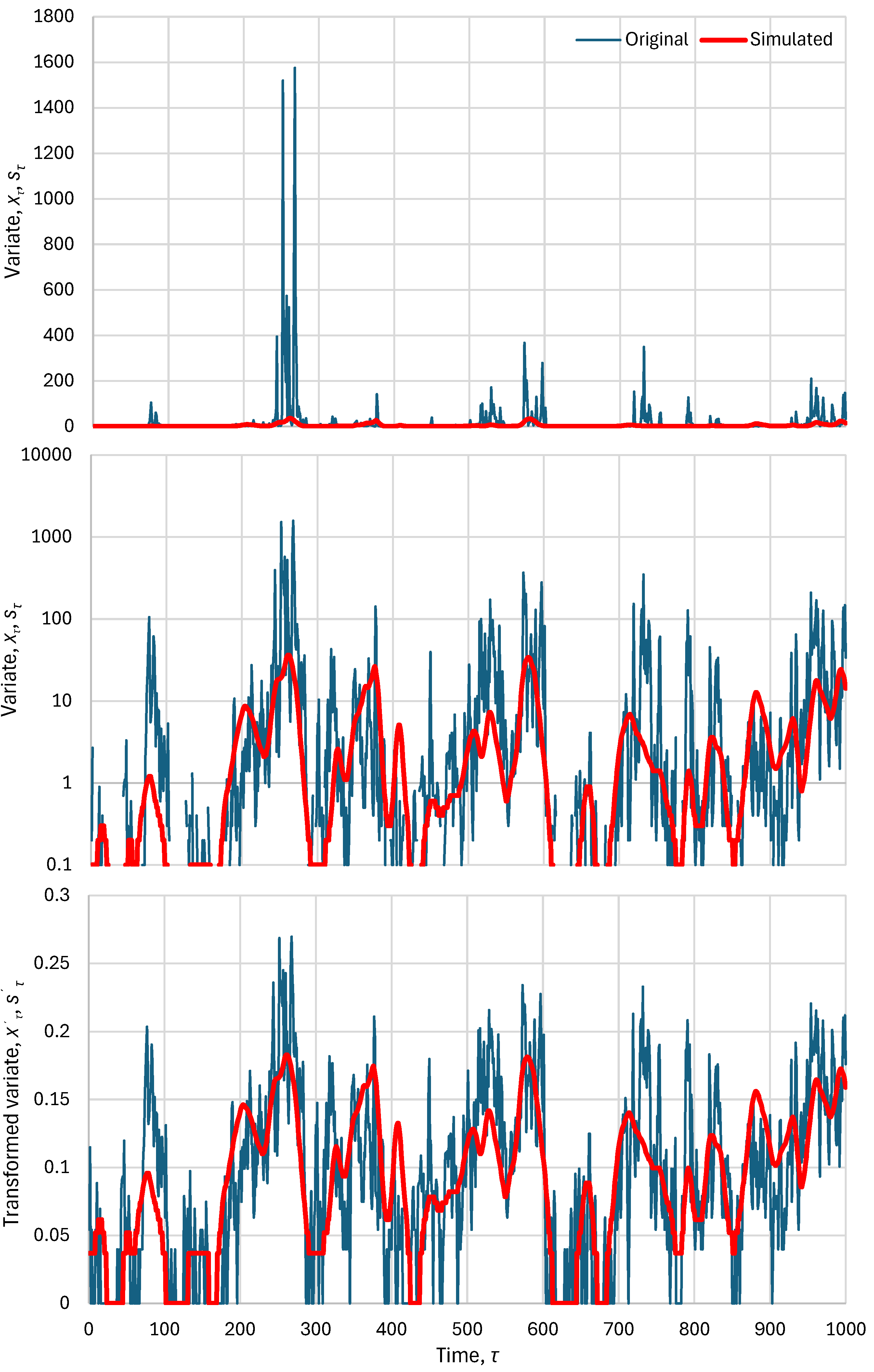
Figure 3.
Performance metrics for the original and finally transformed series (Figure 2, upper and lower, respectively), namely K-explained variance, , as a function of: (left) order for time scale ; (right) time scale for order .
Figure 3.
Performance metrics for the original and finally transformed series (Figure 2, upper and lower, respectively), namely K-explained variance, , as a function of: (left) order for time scale ; (right) time scale for order .
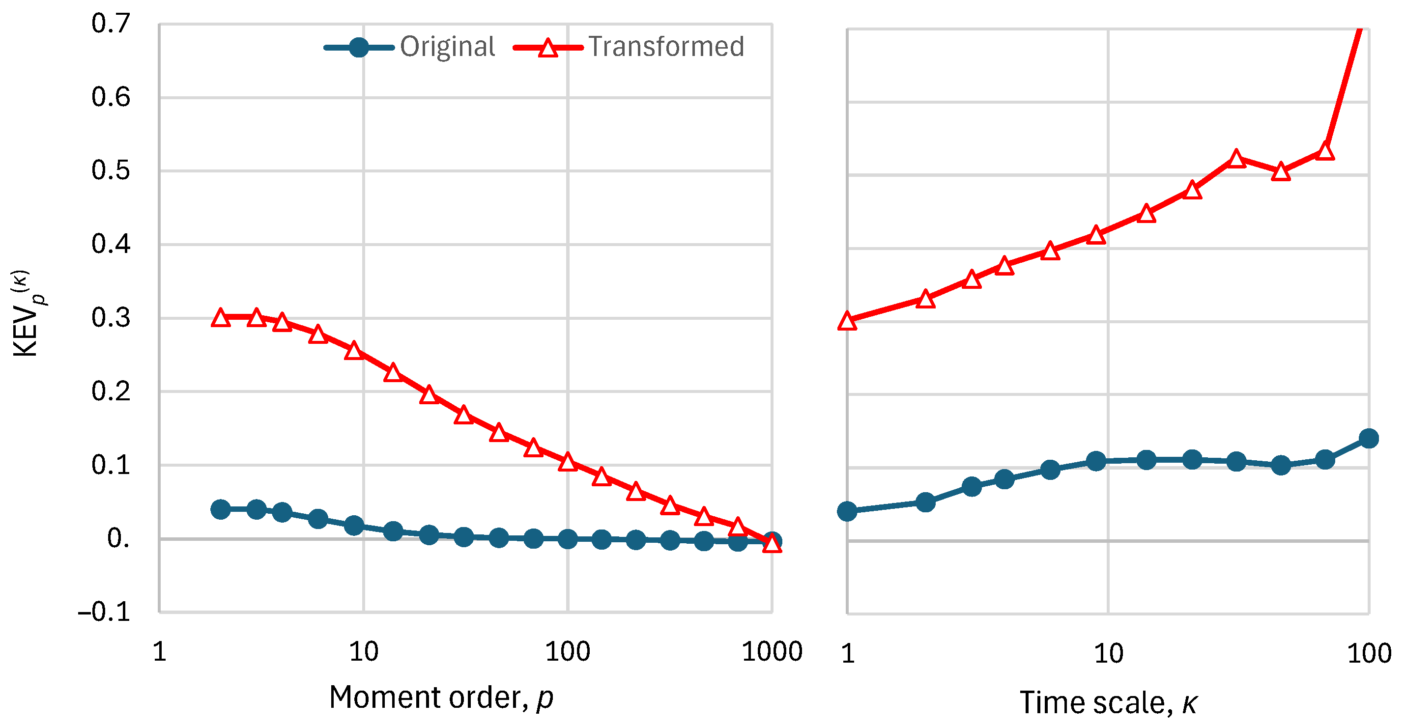
Figure 4.
Model bias metrics for the original and finally transformed series (Figure 2, upper and lower, respectively), as a function of order for time scale : (left) Ratio; (right) K-bias.
Figure 4.
Model bias metrics for the original and finally transformed series (Figure 2, upper and lower, respectively), as a function of order for time scale : (left) Ratio; (right) K-bias.
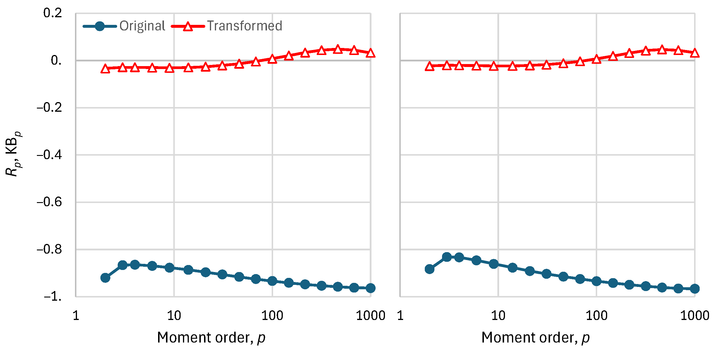
Figure 5.
Spaghetti graphs of modelled annual average precipitation (thin lines) by the 37 CMIP6 GCMs, in comparison to the ERA5 reanalysis data (thick line) for (left) NH and (right) SH.
Figure 5.
Spaghetti graphs of modelled annual average precipitation (thin lines) by the 37 CMIP6 GCMs, in comparison to the ERA5 reanalysis data (thick line) for (left) NH and (right) SH.
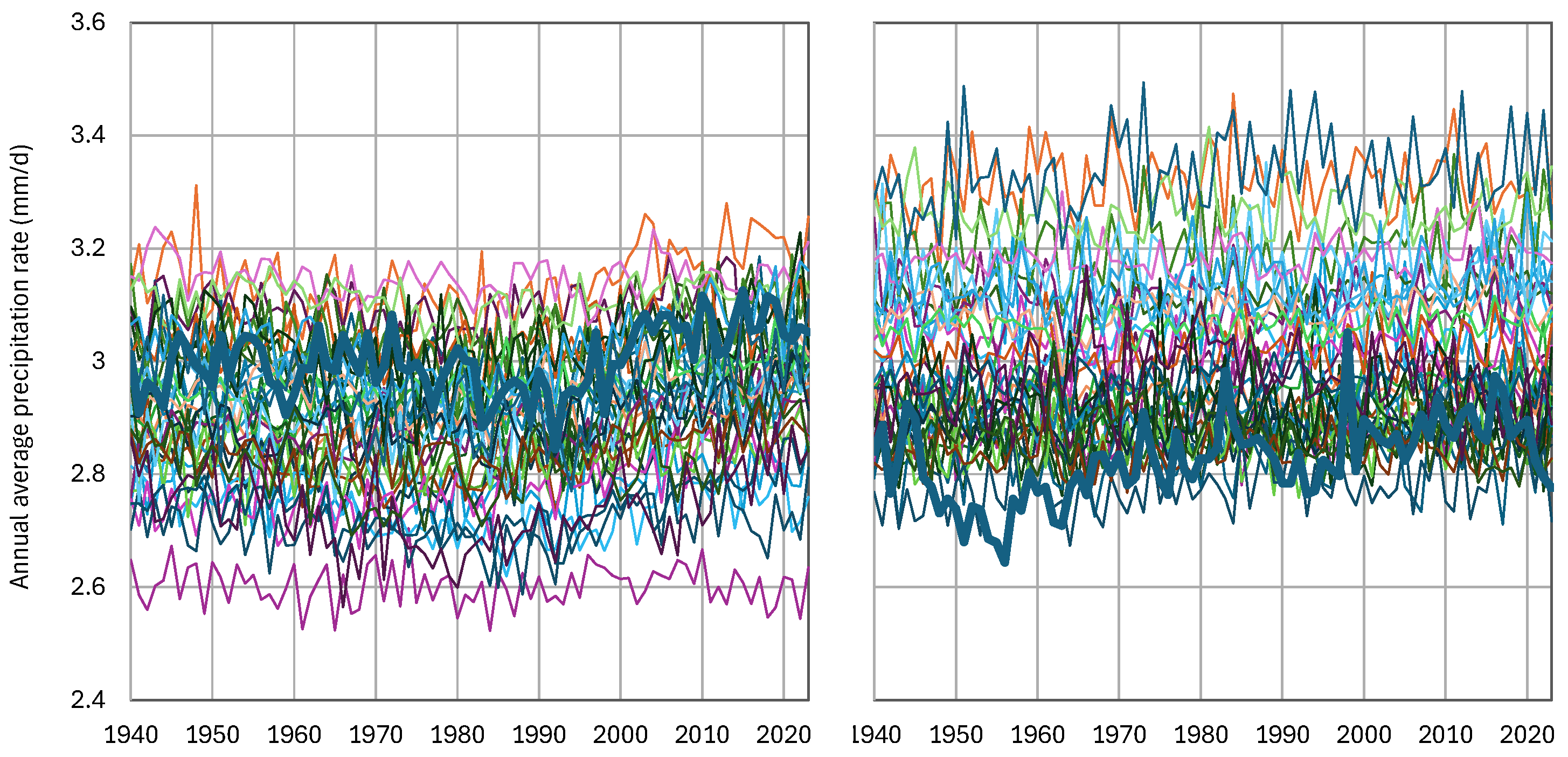
Figure 6.
Spaghetti graphs of modelled 8-year average precipitation (thin lines) by the 37 CMIP6 GCMs, in comparison to the ERA5 reanalysis data (thick line) for (left) NH and (right) SH.
Figure 6.
Spaghetti graphs of modelled 8-year average precipitation (thin lines) by the 37 CMIP6 GCMs, in comparison to the ERA5 reanalysis data (thick line) for (left) NH and (right) SH.
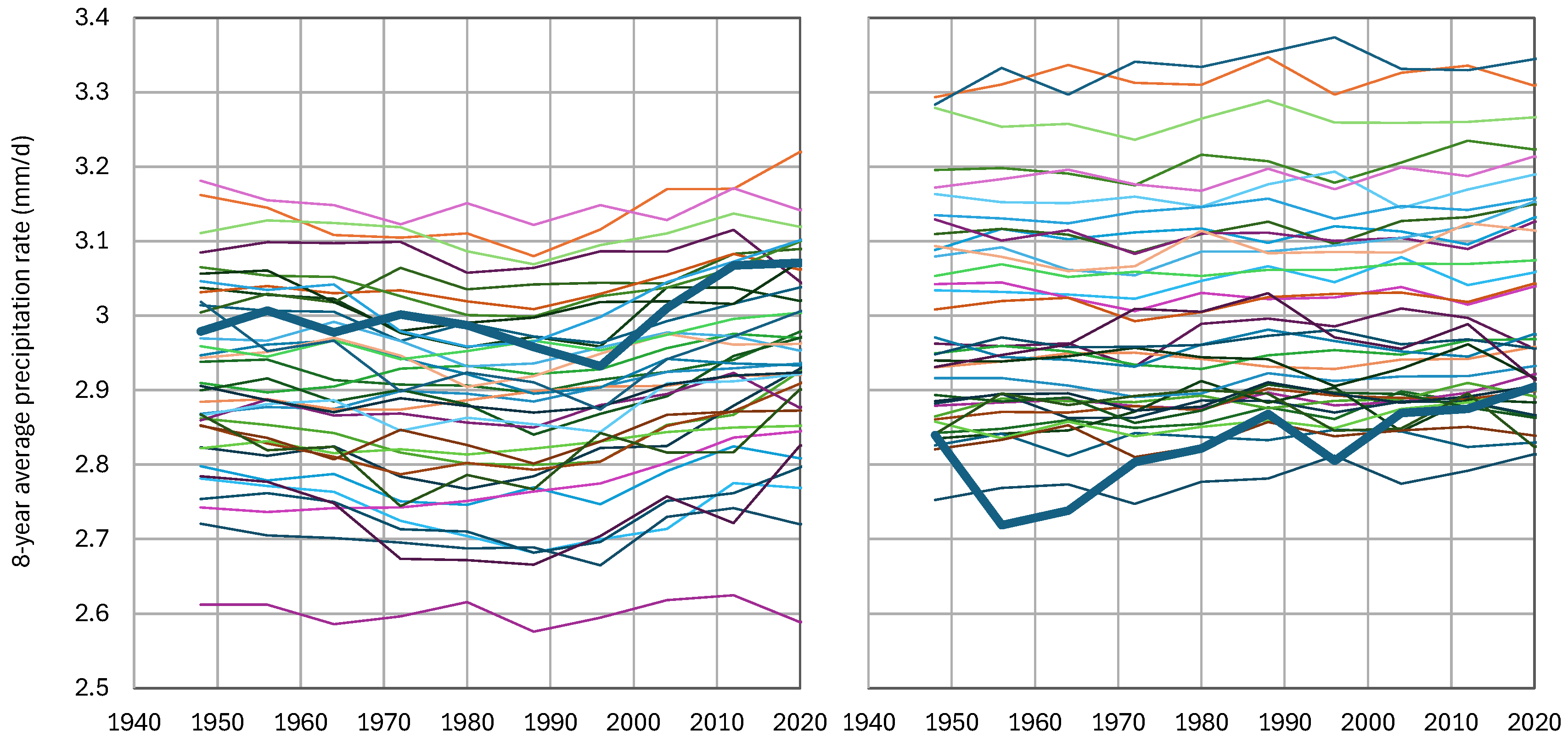
Figure 7.
Box plots of the correlation coefficients between annual time series of (left and middle) GCM models and ERA5 reanalysis for NH and SH, respectively, and (right) the same GCM models for NH and SH. Data points are marked with “◦’ and their mean value with “✕”.
Figure 7.
Box plots of the correlation coefficients between annual time series of (left and middle) GCM models and ERA5 reanalysis for NH and SH, respectively, and (right) the same GCM models for NH and SH. Data points are marked with “◦’ and their mean value with “✕”.
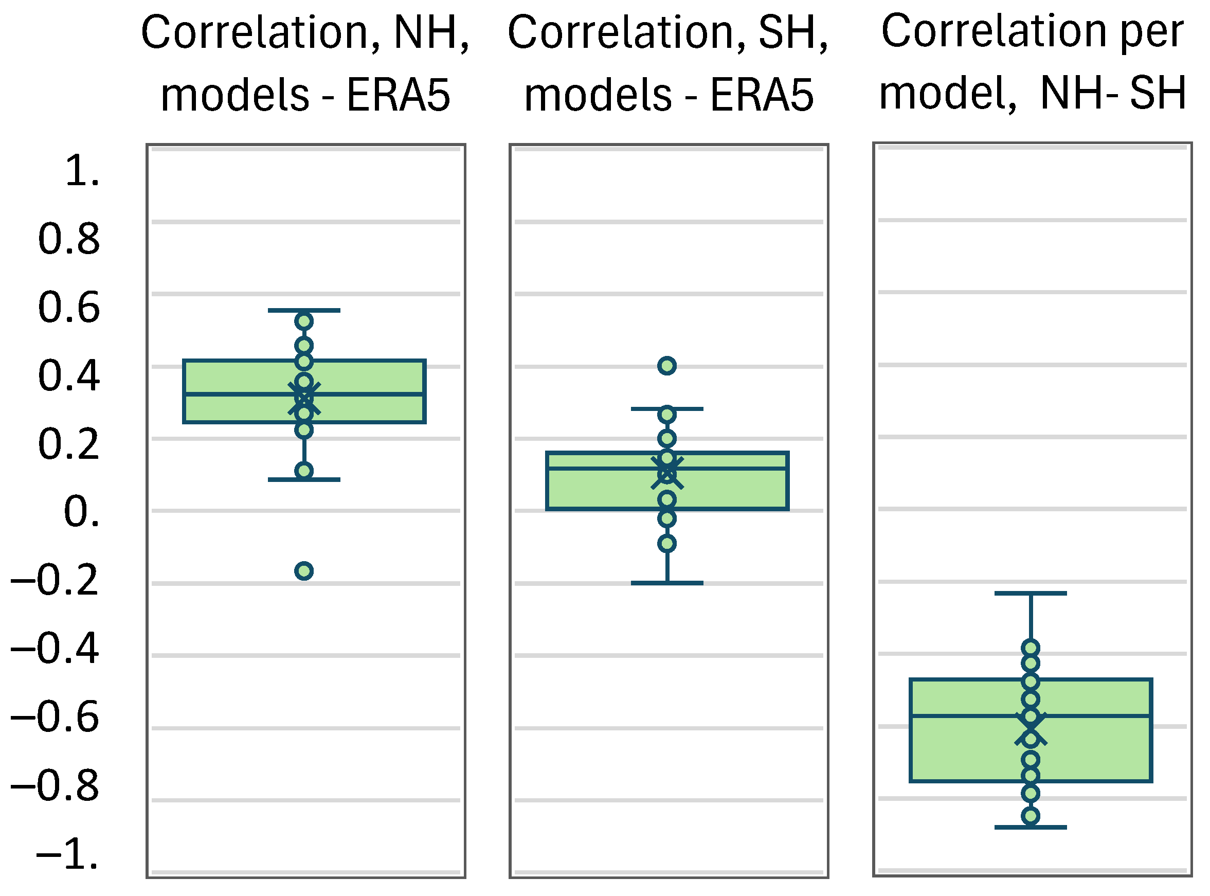
Figure 8.
Box plots of (upper) explained variance, EV, and (lower) K-explained variation, KEV₂, for the indicated cases (NH/SH; annual/8-years scales).
Figure 8.
Box plots of (upper) explained variance, EV, and (lower) K-explained variation, KEV₂, for the indicated cases (NH/SH; annual/8-years scales).
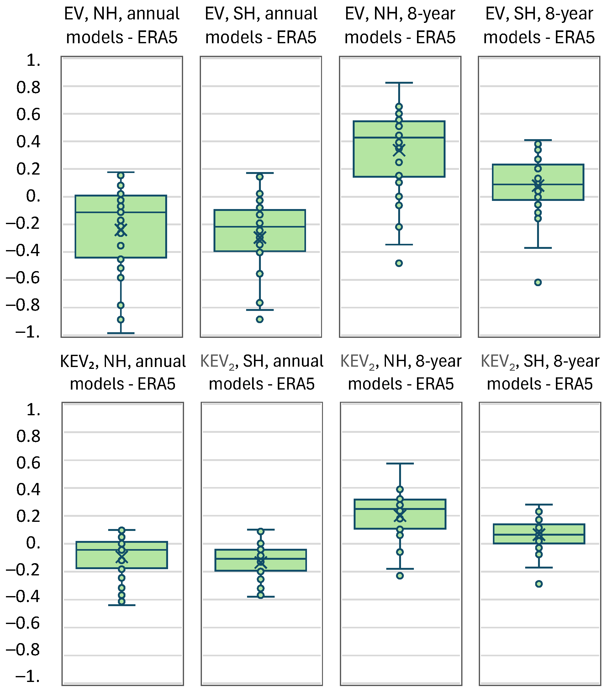
Figure 9.
Box plots of (upper) K-bias, KB₂, (middle) Nash–Sutcliffe efficiency (NSE), and (lower) K-absolute error efficiency, KAEE for the indicated cases (NH/SH; annual/8-years scales).
Figure 9.
Box plots of (upper) K-bias, KB₂, (middle) Nash–Sutcliffe efficiency (NSE), and (lower) K-absolute error efficiency, KAEE for the indicated cases (NH/SH; annual/8-years scales).
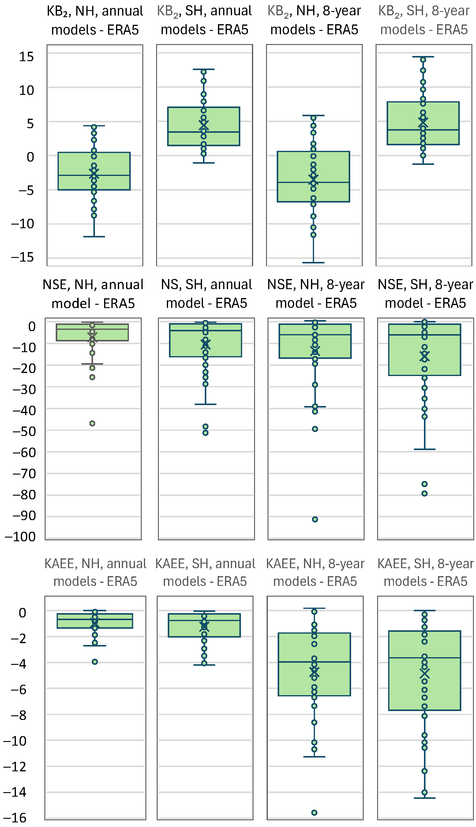
Figure 10.
Cross-performance at both hemispheres of the GCMs, in terms of K-explained variation, KEV₂, at time scales (left) annual; (right) 8-year.
Figure 10.
Cross-performance at both hemispheres of the GCMs, in terms of K-explained variation, KEV₂, at time scales (left) annual; (right) 8-year.
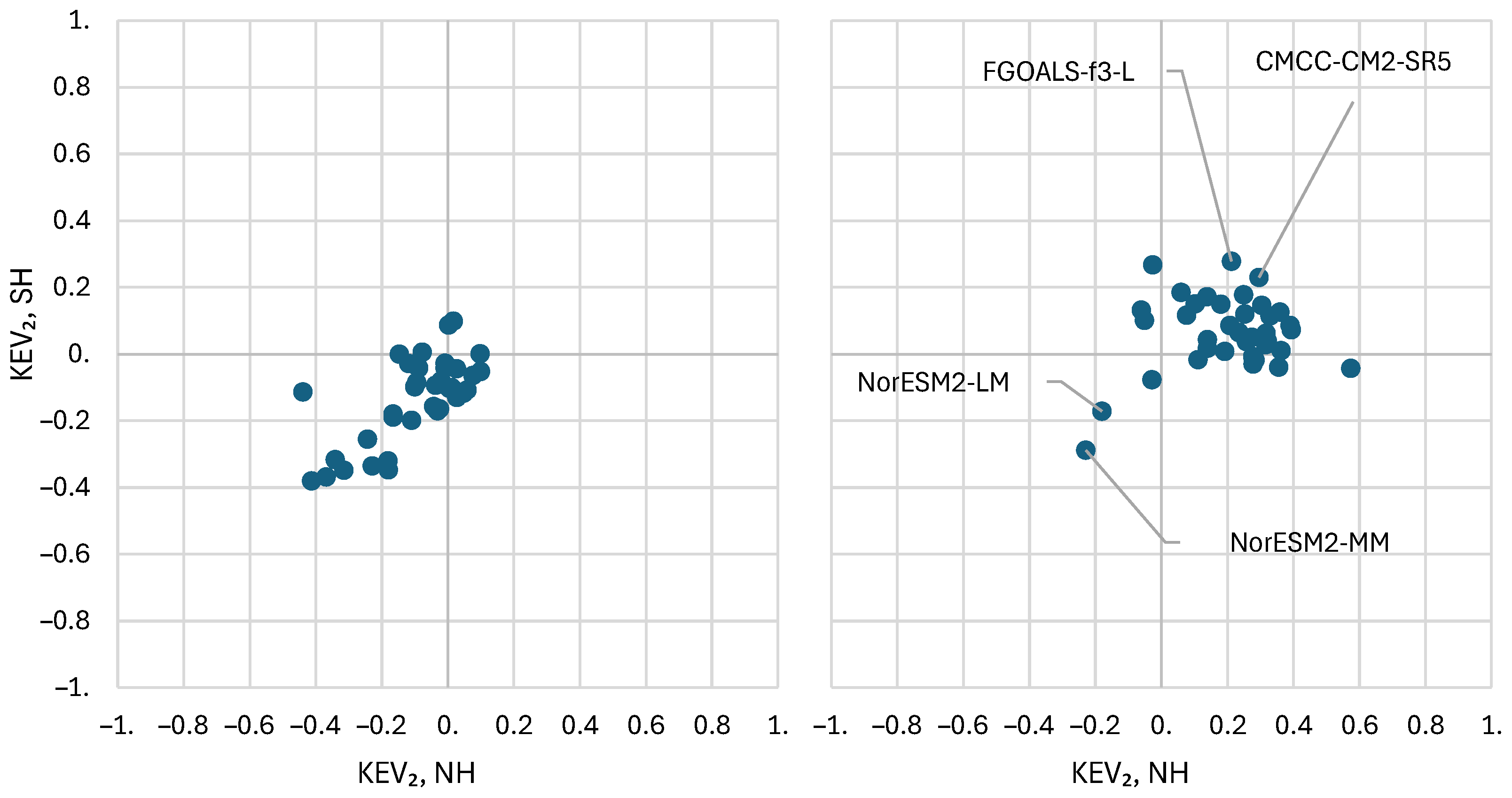
Figure 11.
Performance metrics of the CMCC-CM2-SR5 for the NH and SH, namely K-explained variance, , as a function of: (left) order for time scale ; (right) time scale for order .
Figure 11.
Performance metrics of the CMCC-CM2-SR5 for the NH and SH, namely K-explained variance, , as a function of: (left) order for time scale ; (right) time scale for order .
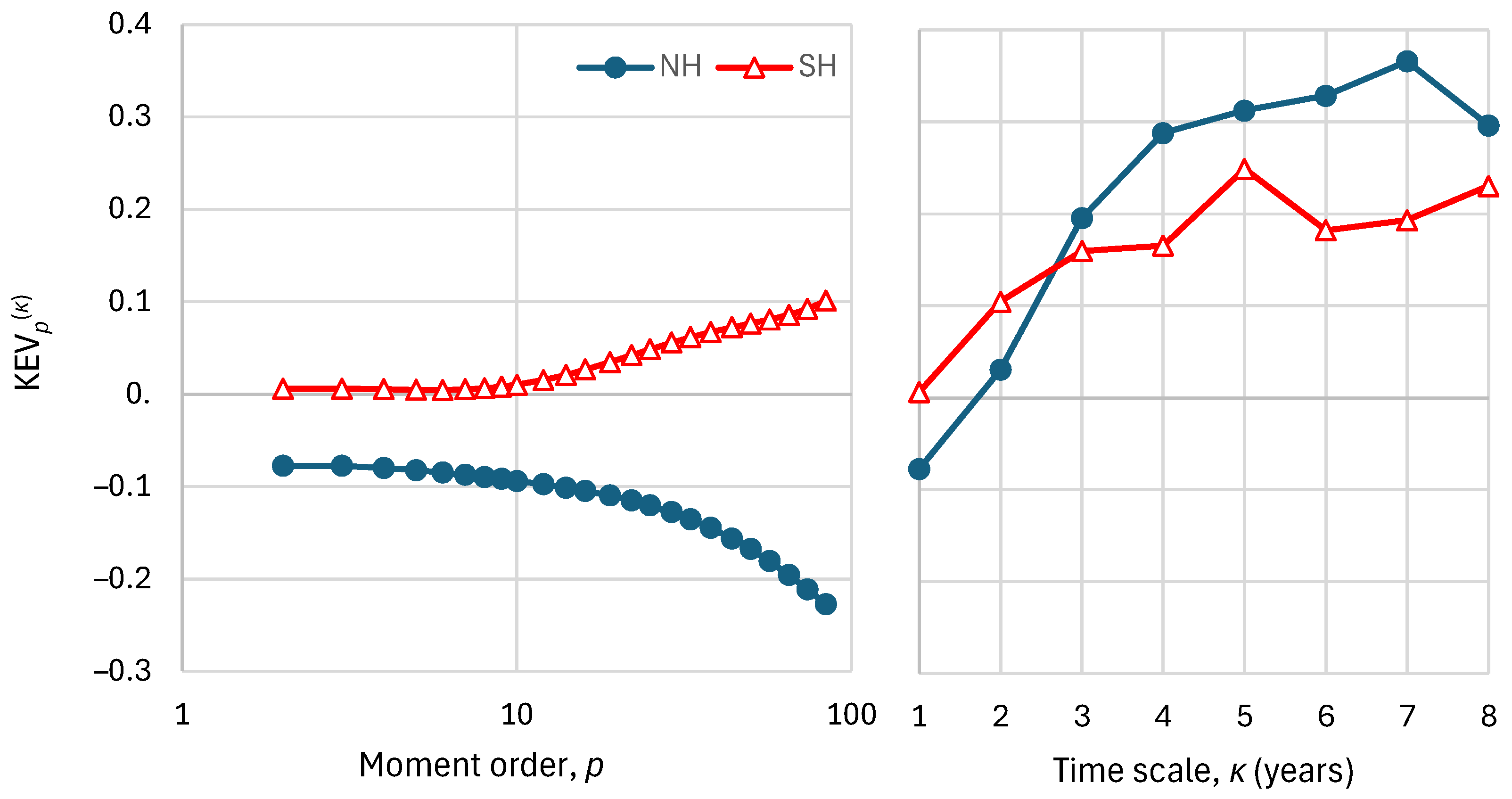
Figure 12.
Performance metrics of the CMCC-CM2-SR5 for the NH and for the original and transformed series, namely K-explained variance, , as a function of: (left) order for time scale ; (right) time scale for order .
Figure 12.
Performance metrics of the CMCC-CM2-SR5 for the NH and for the original and transformed series, namely K-explained variance, , as a function of: (left) order for time scale ; (right) time scale for order .
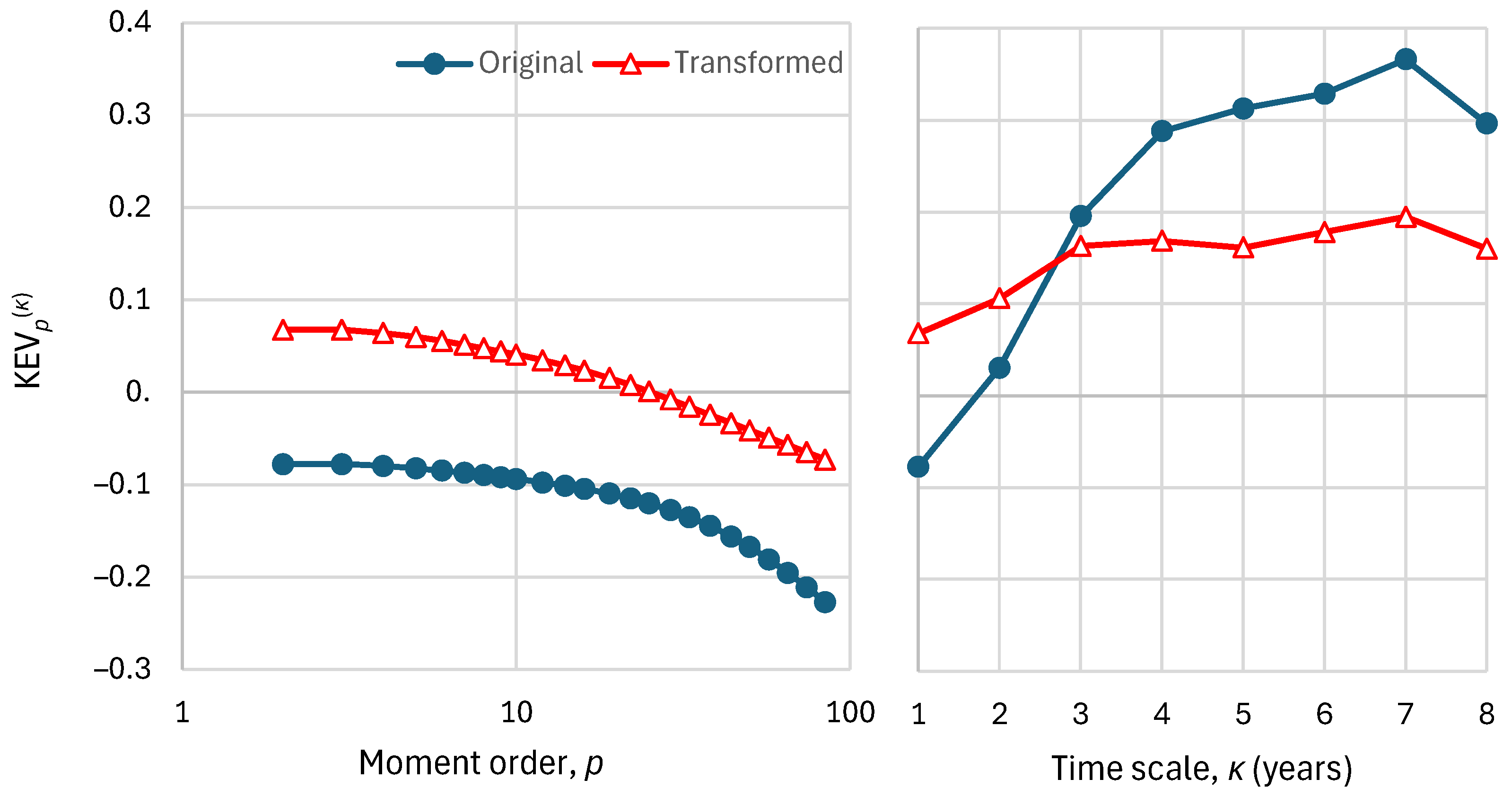
Figure 13.
Evolution of the precipitation in the wider area of Europe, defined by the coordinates 11° W 40° E, 34 N° 71° N at (left) annual and (right) 8-year time scale, in comparison to the “best performing” GCMs, namely CMCC-CM2-SR5 and FGOALS-f3-L.
Figure 13.
Evolution of the precipitation in the wider area of Europe, defined by the coordinates 11° W 40° E, 34 N° 71° N at (left) annual and (right) 8-year time scale, in comparison to the “best performing” GCMs, namely CMCC-CM2-SR5 and FGOALS-f3-L.
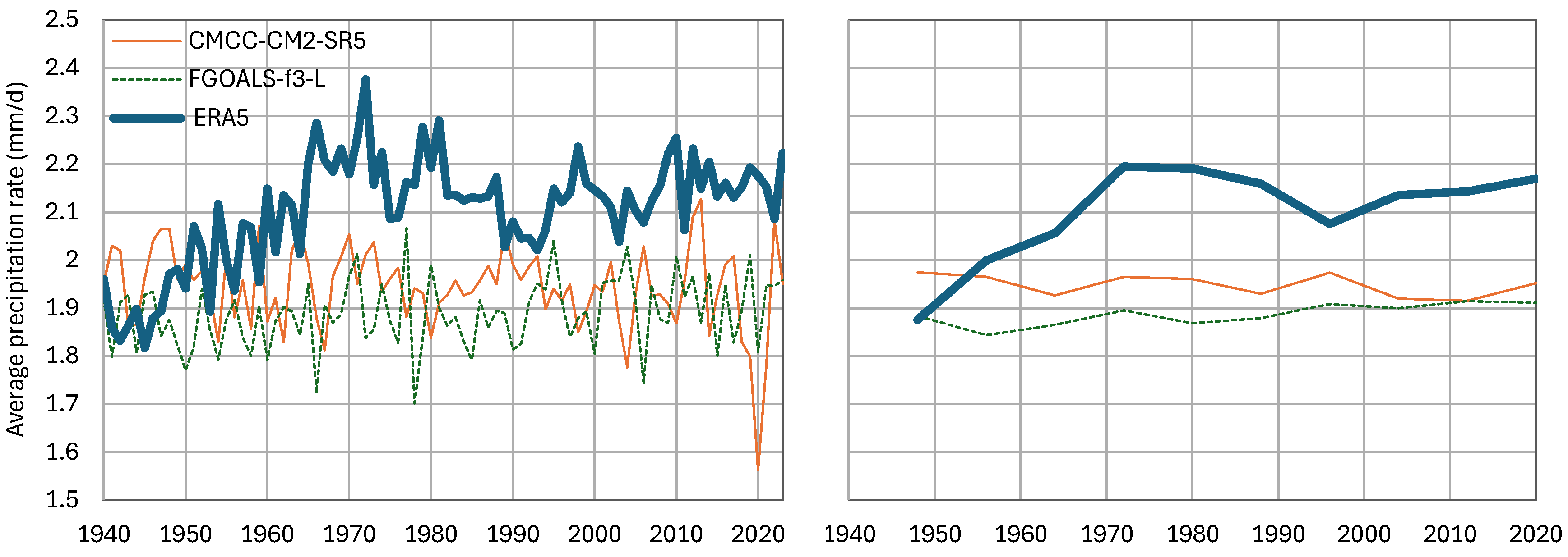
Figure 14.
Performance metrics of the “best performing” GCMs, namely CMCC-CM2-SR5 and FGOALS-f3-L for the wider area of Europe, based on the time series seen in Figure 13, namely K-explained variance, , as a function of: (left) order for time scale ; (right) time scale for order .
Figure 14.
Performance metrics of the “best performing” GCMs, namely CMCC-CM2-SR5 and FGOALS-f3-L for the wider area of Europe, based on the time series seen in Figure 13, namely K-explained variance, , as a function of: (left) order for time scale ; (right) time scale for order .
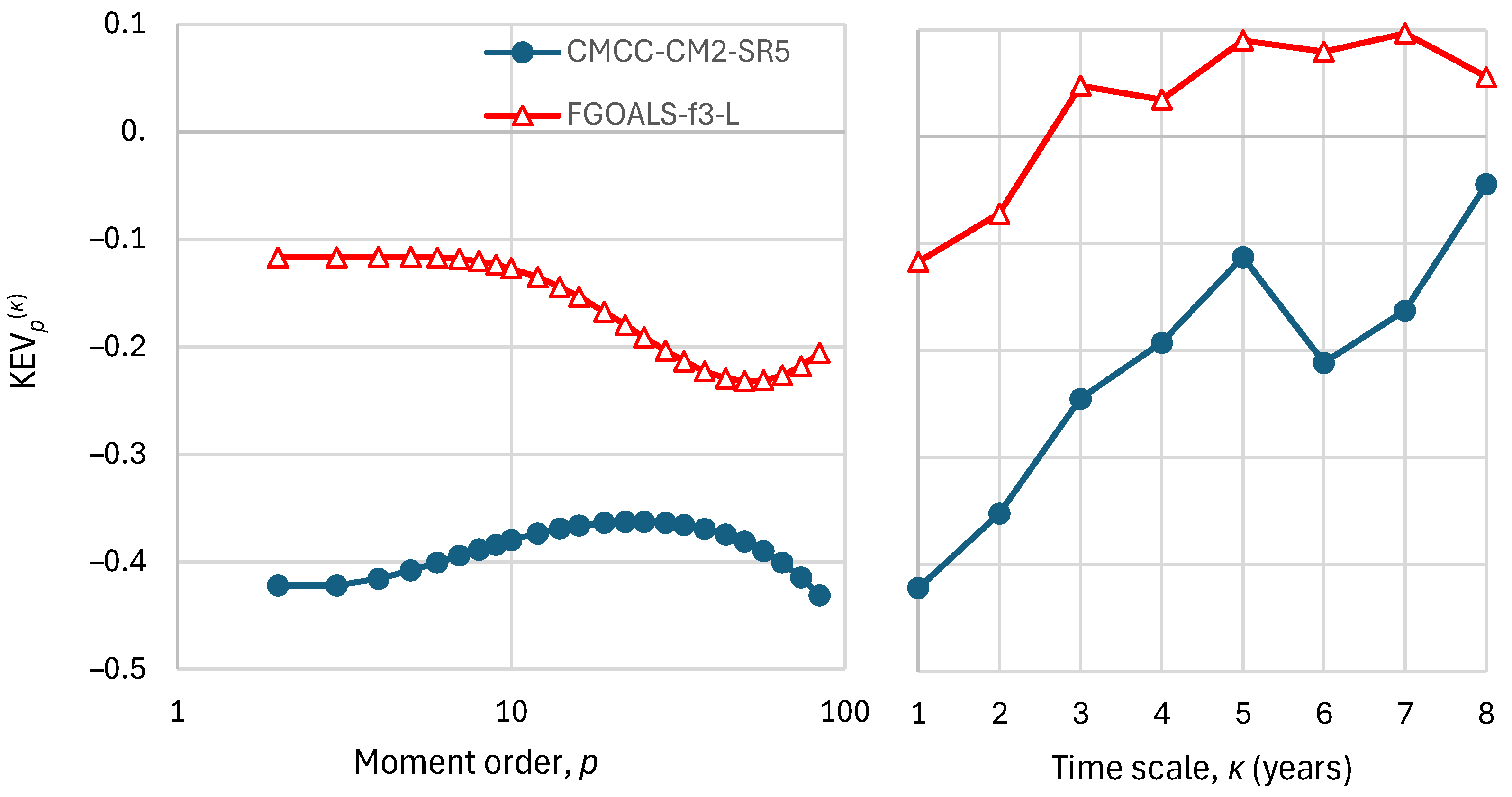

Table 1.
Model efficiency metrics and fitted parameters of transformations for the example depicted on Figure 2.
Table 1.
Model efficiency metrics and fitted parameters of transformations for the example depicted on Figure 2.
| Site | λ | α | β | r | EV | CB | NSE | KGE | KEV₂ | KB2 | AEE |
| Untransformed | 0.364 | 0.049 | –0.167 | 0.022 | –0.371 | 0.040 | –0.921 | –0.160 | |||
| Log transformed | 0.708 | 0.498 | –0.001 | 0.498 | 0.631 | 0.297 | –0.002 | 0.297 | |||
| λ transformed | 0.044 | 0 | 1 | 0.708 | 0.486 | –0.131 | 0.477 | 0.656 | 0.292 | –0.233 | 0.273 |
| λ transformed | 0.024 | –0.005 | 1.057 | 0.714 | 0.504 | –0.019 | 0.504 | 0.649 | 0.302 | –0.033 | 0.301 |
Table 2.
The CMIP6 climate models (GCMs) whose results are used in this study.
| # | CMIP6 GCM | # | CMIP6 GCM | # | CMIP6 GCM | # | CMIP6 GCM |
| 1 | ACCESS-CM2 | 11 | CIESM | 21 | GFDL-CM4 | 31 | MPI-ESM1-2-HR |
| 2 | ACCESS-ESM1-5 | 12 | CMCC-CM2-SR5 | 22 | GFDL-ESM4 | 32 | MPI-ESM1-2-LR |
| 3 | AWI-CM-1-1-MR | 13 | CNRM-CM6-1 f2 | 23 | GISS-E2-1-G-p3 | 33 | MRI-ESM2-0 |
| 4 | BCC-CSM2-MR | 14 | CNRM-CM6-1-HR f2 | 24 | HadGEM3-GC31-LL f3 | 34 | NESM3 |
| 5 | CAMS-CSM1-0 | 15 | CNRM-ESM2-1-f2 | 25 | INM-CM4-8 | 35 | NorESM2-LM |
| 6 | CanESM5 p2 | 16 | EC-Earth3 | 26 | INM-CM5-0 | 36 | NorESM2-MM |
| 7 | CanESM5-CanOE p2 | 17 | EC-Earth3-Veg | 27 | IPSL-CM6A-LR | 37 | UKESM1-0-LL f2 |
| 8 | CanESM5-p1 | 18 | FGOALS-f3-L | 28 | KACE-1-0-G | ||
| 9 | CESM2 | 19 | FGOALS-g3 | 29 | MIROC6 | ||
| 10 | CESM2-WACCM | 20 | FIO-ESM-2-0 | 30 | MIROC-ES2L f2 |
Disclaimer/Publisher’s Note: The statements, opinions and data contained in all publications are solely those of the individual author(s) and contributor(s) and not of MDPI and/or the editor(s). MDPI and/or the editor(s) disclaim responsibility for any injury to people or property resulting from any ideas, methods, instructions or products referred to in the content. |
© 2024 by the authors. Licensee MDPI, Basel, Switzerland. This article is an open access article distributed under the terms and conditions of the Creative Commons Attribution (CC BY) license (http://creativecommons.org/licenses/by/4.0/).
Copyright: This open access article is published under a Creative Commons CC BY 4.0 license, which permit the free download, distribution, and reuse, provided that the author and preprint are cited in any reuse.


