
Submitted:
12 December 2024
Posted:
12 December 2024
You are already at the latest version
Abstract
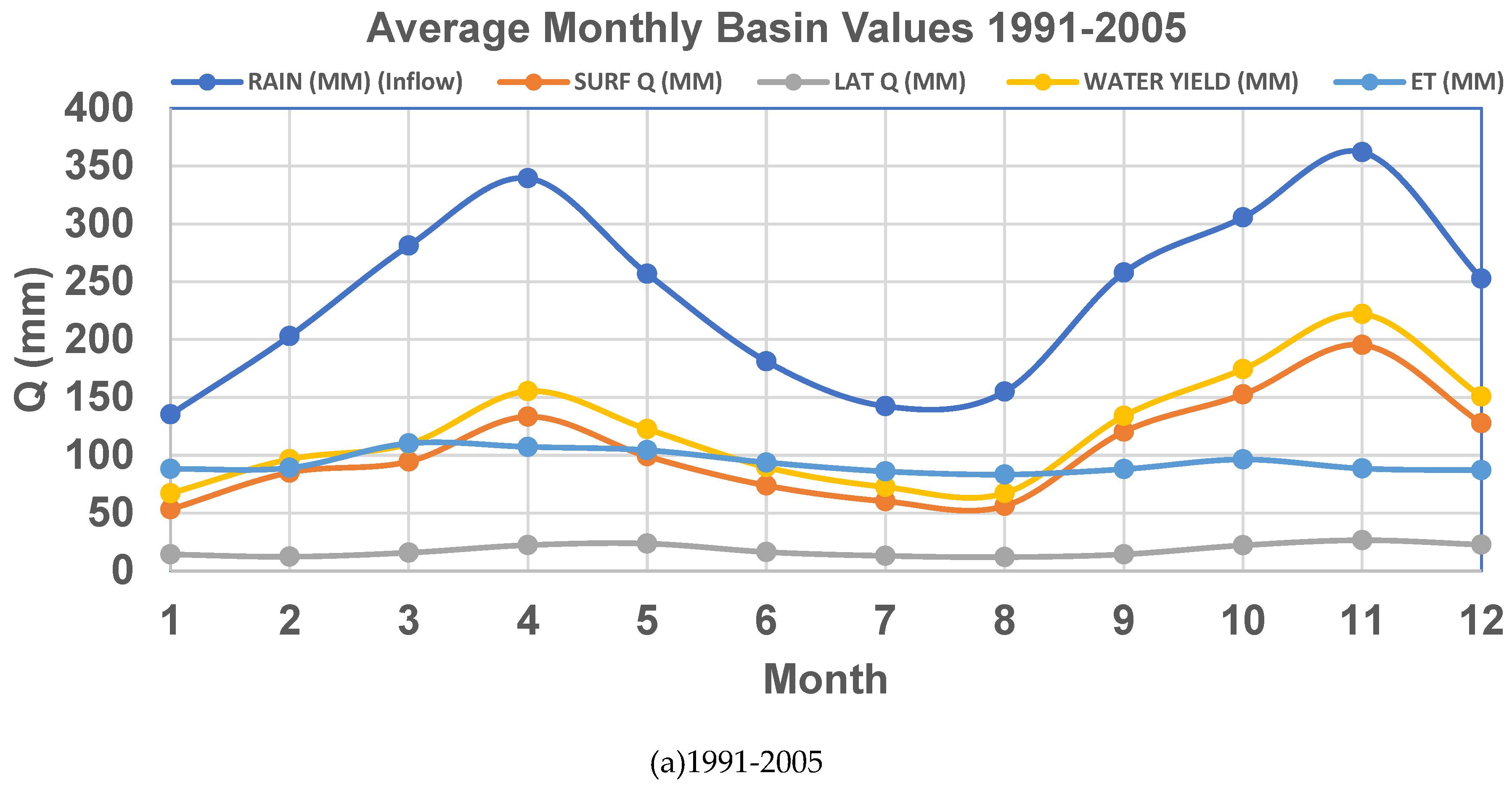
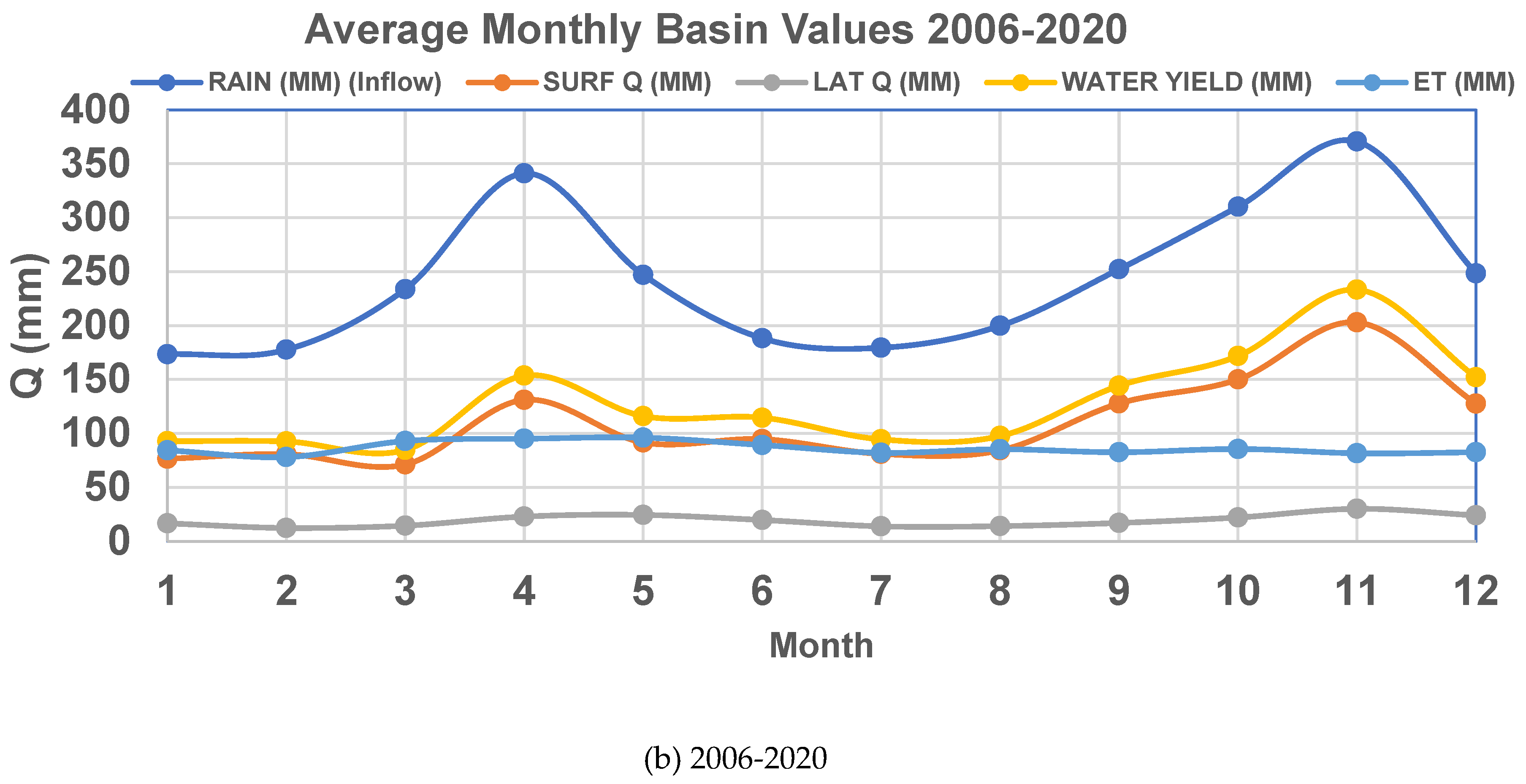
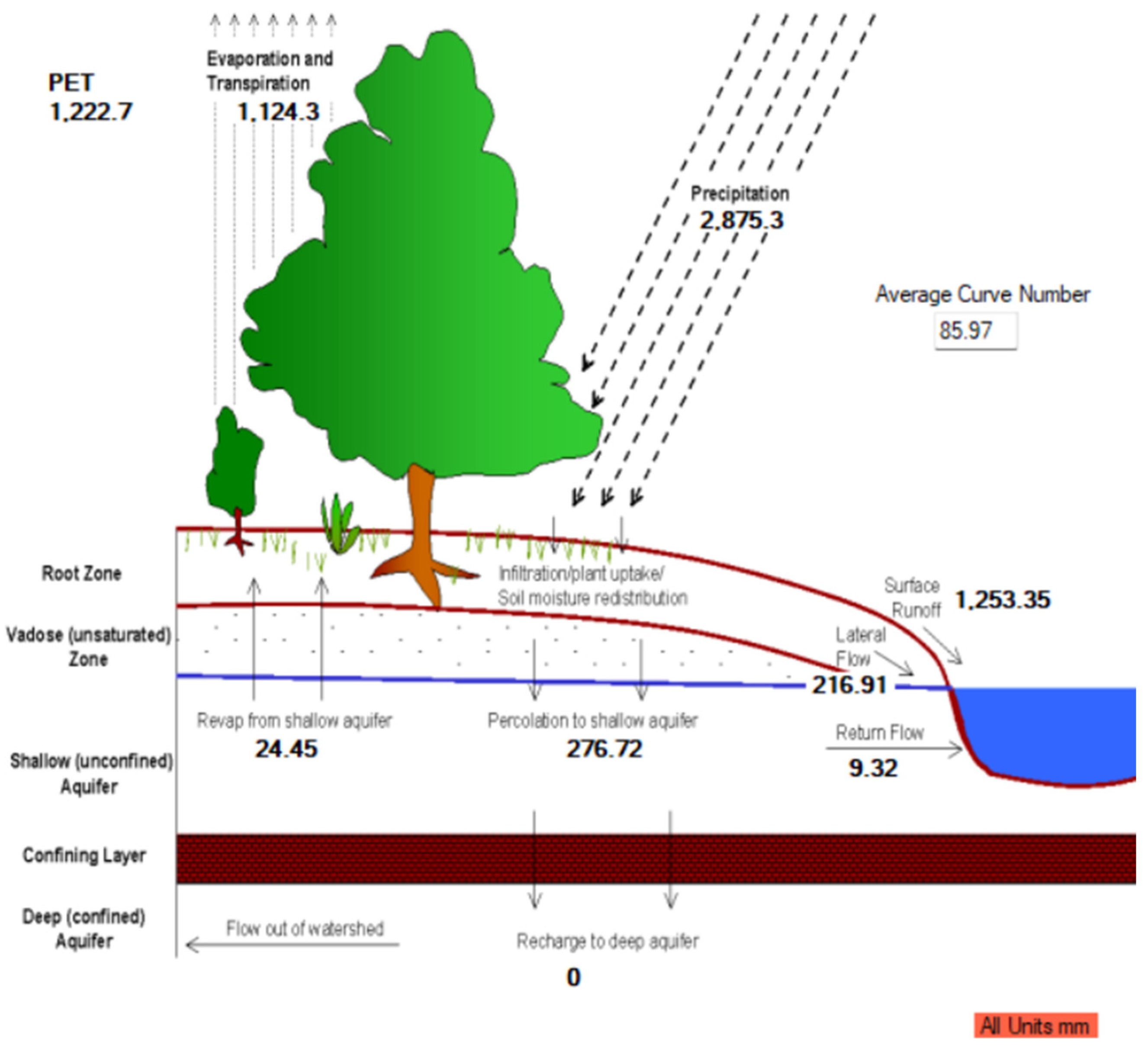
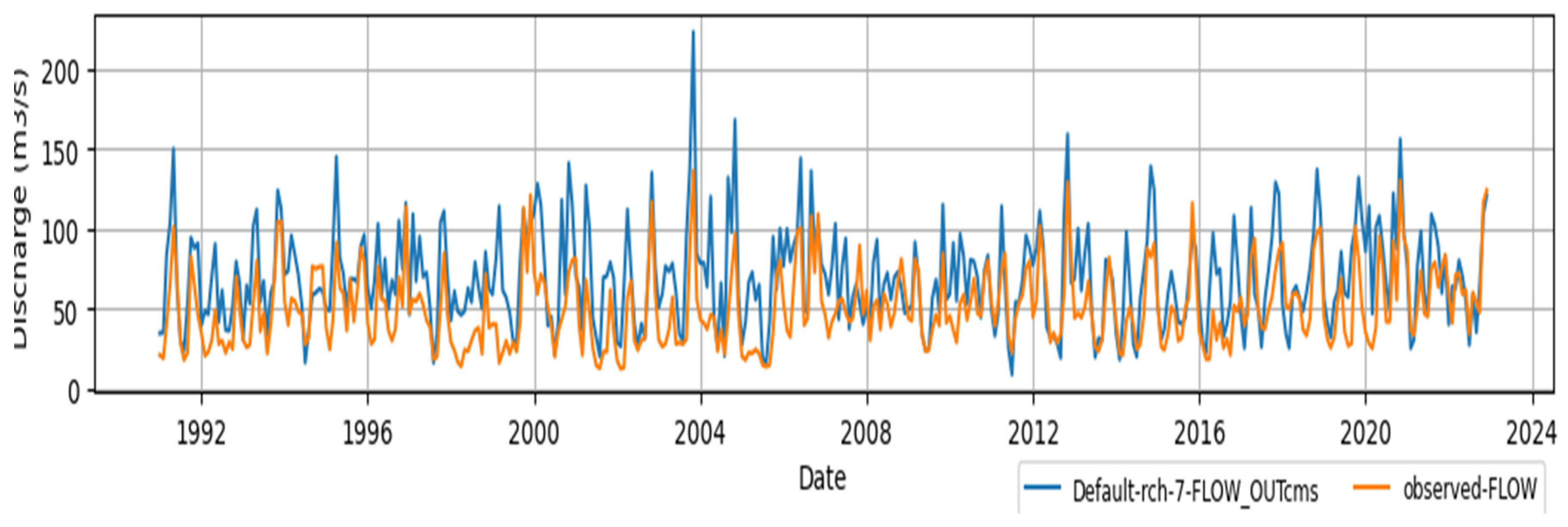
Enhancing sustainable agricultural practices and water resources management calls for this study, which focuses on calibrating and validating the SWAT model using data from CMIP6. The SWAT model was validated using Bernam streamflow data from 1985-2022, divided into three categories: category 1 (10 years calibration- and 5 years validation), category 2 (15 years calibration- and 10 years validation), and category 3. The SWAT model performed "GOOD" in the Bernam watershed, as indicated by statistical analysis during calibration and validation phases, utilizing statistical indices. The results for the p-factor, r-factor, R2, NSE, PBIAS, and KGE were 0.82, 0.88, 0.72, 0.70, -1.1%, and 0.85 during the calibration period and 0.8, 1.04, 0.75, 0.65, -6.6%, and 0.79 during the validation period. The result of the simulation after adjusting the SWAT model parameters with calibrated best-fit values indicated that the inflow (rainfall) and the outflow (water yield + ET) are 2,873.36mm and 2,592.78mm respectively, with difference of 9.8% for the period of 1991-2005 while 2,921.98 mm and 2,586.07 mm for the inflow and outflow, during 2006-2020 period with difference of 11.5%. The SWAT model effectively predicts agro-hydrological processes, aiding decision-makers in UBRB's agricultural water management and guiding sustainable agriculture through advanced climate projections.
Keywords:
1. Introduction
2. Materials and Methods
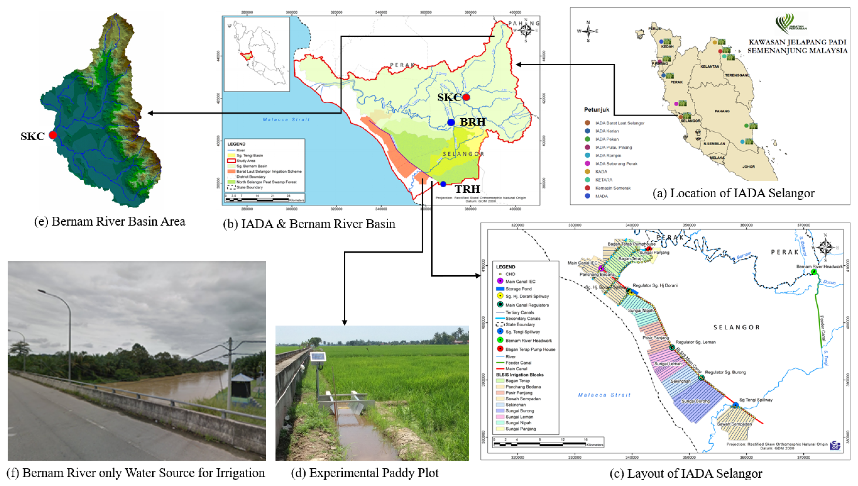
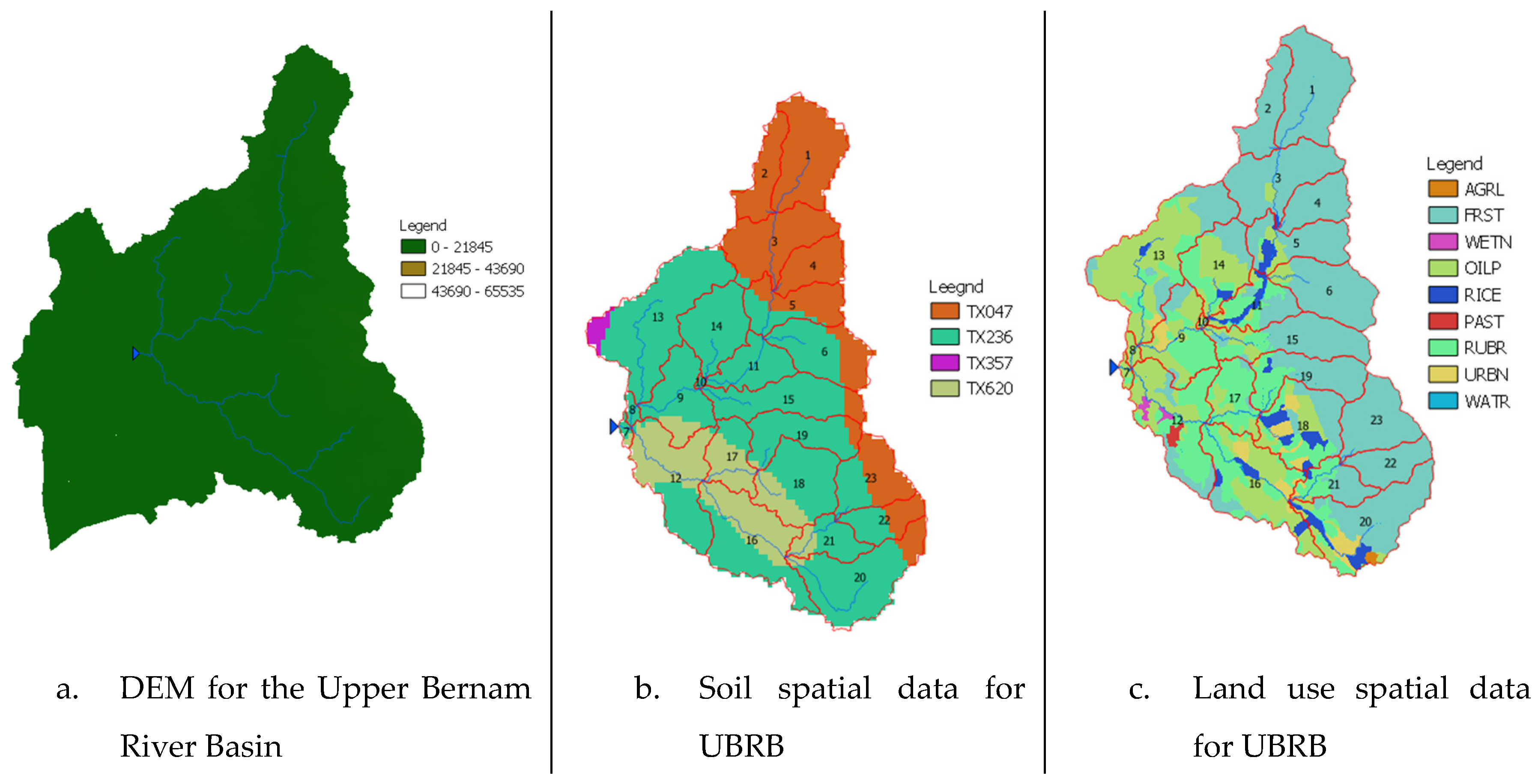
2.1. Study Area
2.2. SWAT and SWAT-CUP
2.3. SWAT Model Data and Setup
2.4. Calibration and Validation of the SWAT-CUP
3. Results
3.1. Parameter Sensitivity Analysis

| S/N | Parameter code | Parameter description | Object type | Range | "Best fit"-Values | t-Stat | P-Value | Method |
|---|---|---|---|---|---|---|---|---|
| 1 | CN2 | SCS runoff curve number | mgt | -0.2-0.2 | 0.082182 | -23.4601 | 0 | r |
| 2 | ESCO | Soil evaporation compensation factor. | hru | 0-1 | 0.149648 | -12.3956 | 0 | v |
| 3 | ALPHA_BNK | Baseflow alpha factor for bank storage. | rte | 0-1 | 0.18104 | -8.28811 | 0 | v |
| 4 | CANMX | Maximum canopy storage. | hru | 0-100 | 31.875715 | 5.781076 | 1.3E-08 | v |
| 5 | HRU_SLP | Average slope steepness | hru | 0-0.7 | 0.645705 | -4.60945 | 5.2E-06 | v |
| 6 | SUB_ELEV | Elevation of subbasin | sub | 0-6,000 | 5643.671387 | 4.377764 | 1.48E-05 | v |
| 7 | GWQMN | Minimum water depth in the shallow aquifer needed for return flow to happen (mm). | gw | 0-10,000 | 9160.946289 | 3.190084 | 0.001517 | v |
| 8 | CH_N2 | Manning’s "n" value for the main channel. | rte | -0.01-0.3 | -0.073626 | 3.12361 | 0.001896 | v |
| 9 | RCHRG_DP | Deep aquifer percolation fraction. | gw | 0-1 | 0.236758 | 2.918687 | 0.003683 | r |
| 10 | CH_K2 | Effective hydraulic conductivity in main channel alluvium. | rte | -0.01-1,000 | 753.380676 | 2.61088 | 0.009318 | v |
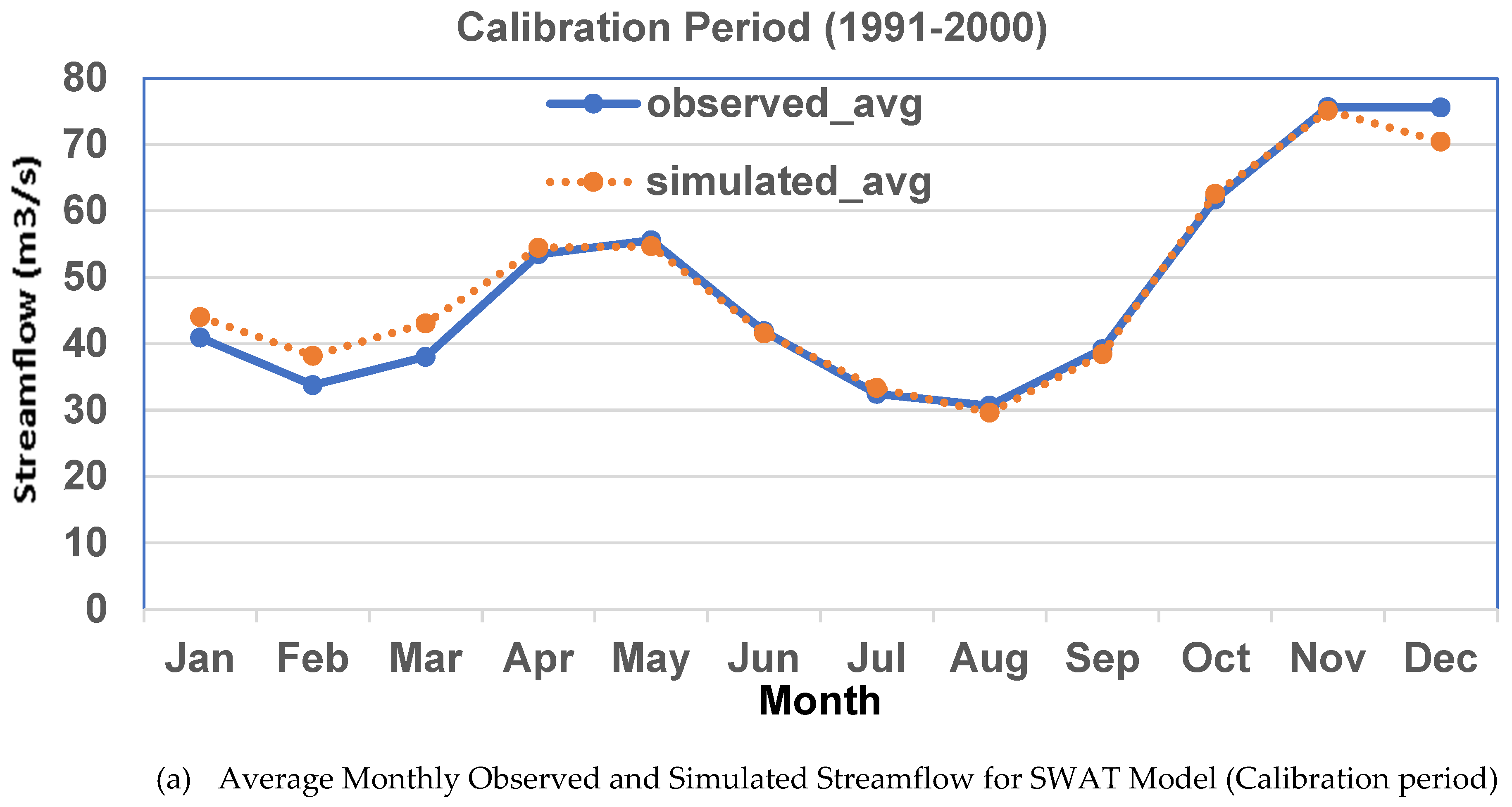
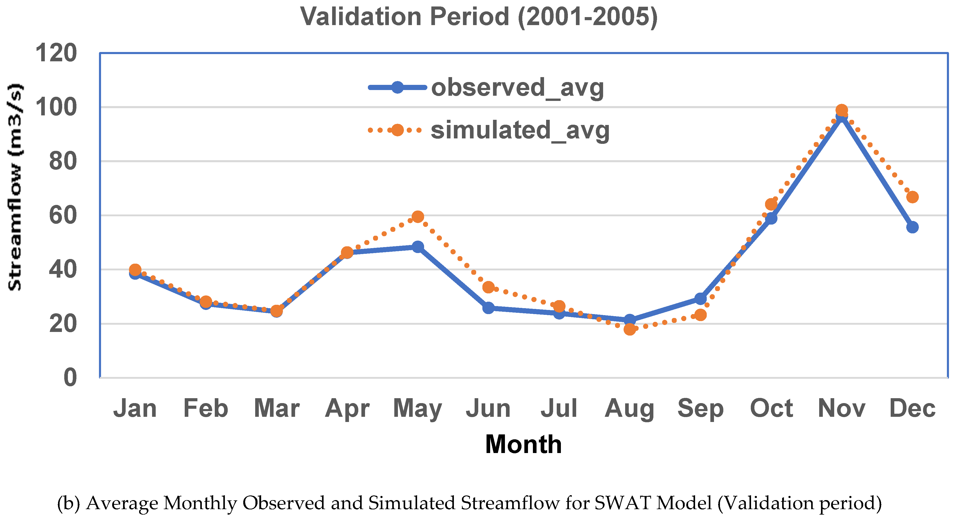
3.2. SWAT Calibration and Validation
| Period | Set | Settings | Variable | p-factor | r-factor | R2 | NS | bR2 | MSE | SSQR | PBIAS | KGE | RSR | MNS | VOL_FR | Mean_sim | Mean_obs | StdDev_sim | StdDev_obs | STATUS |
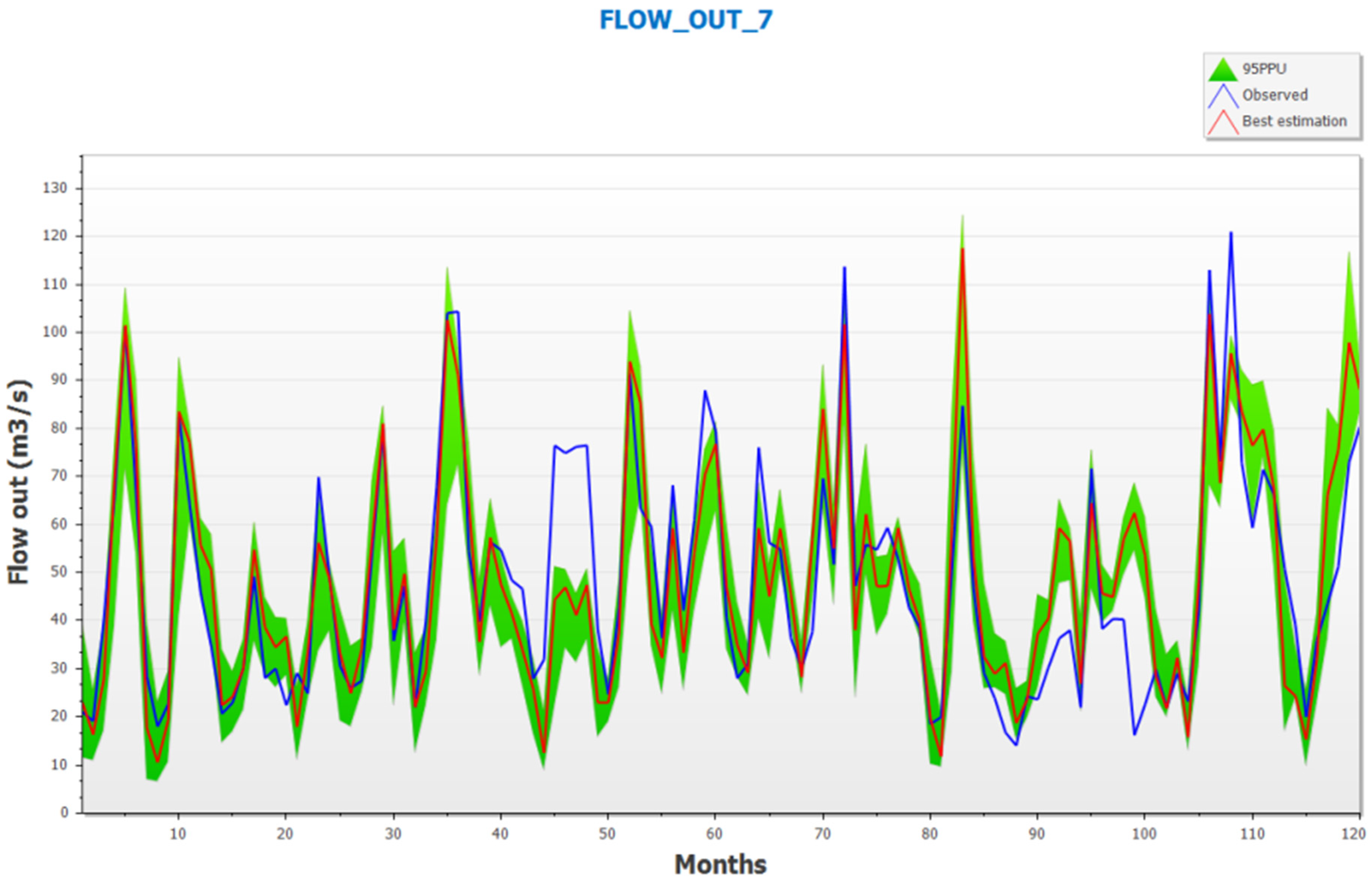
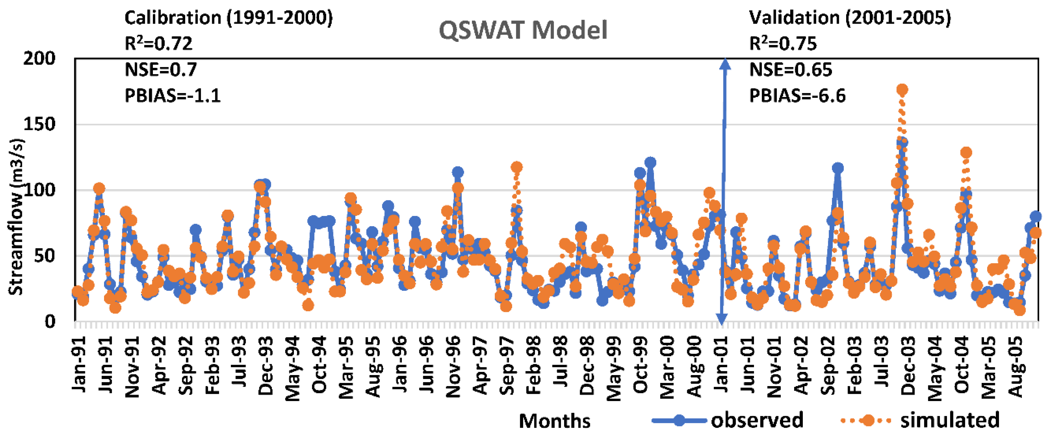
| Cal-1991-2000 | SET1 | Iter1_3=600 | FLOW_OUT_7 | 0.82 | 0.88 | 0.72 | 0.7 | 0.6147 | 1.70E+02 | 8.30E+00 | -1.1 | 0.85 | 0.55 | 0.5 | 0.99 | 48.79 | 48.24 | 23.85 | 23.81 | New Par of Iter1_2 |
| Val-2001-2005 | SET1 | VAL2001-2005 | FLOW_OUT_7 | 0.8 | 1.04 | 0.75 | 0.65 | 0.7376 | 2.40E+02 | 3.90E+01 | -6.6 | 0.79 | 0.59 | 0.46 | 0.94 | 44.08 | 48.24 | 30.05 | 23.81 | New Par of Iter1_2 |
| Cal-1991-2000 | SET2 | Iter1_3=600 | FLOW_OUT_7 | 0.68 | 1.17 | 0.73 | 0.73 | 0.5127 | 1.50E+02 | 2.80E+01 | -2.7 | 0.77 | 0.52 | 0.52 | 0.97 | 49.53 | 48.24 | 19.44 | 23.81 | New Par of Iter1_2 |
| Val-2001-2005 | SET2 | VAL2001-2005 | FLOW_OUT_7 | 0.45 | 1.14 | 0.73 | 0.62 | 0.6039 | 2.60E+02 | 8.40E+01 | -19.4 | 0.76 | 0.61 | 0.35 | 0.84 | 49.37 | 41.33 | 25.36 | 26.22 | New Par of Iter1_2 |
| Cal-2001-2010 | SET1 | Iter1_3=600 | FLOW_OUT_7 | 0.78 | 1.3 | 0.62 | 0.6 | 0.4583 | 2.30E+02 | 2.30E+01 | -1.9 | 0.78 | 0.63 | 0.37 | 0.98 | 48.83 | 47.93 | 22.6 | 24.21 | New Par of Iter1_2 |
| Val-2011-2015 | SET1 | VAL2011-2015 | FLOW_OUT_7 | 0.75 | 1.29 | 0.78 | 0.66 | 0.6701 | 2.00E+02 | 7.30E+01 | 14.7 | 0.81 | 0.58 | 0.42 | 1.17 | 45.19 | 52.99 | 23.61 | 24.04 | New Par of Iter1_2 |
| Cal-2001-2010 | SET2 | Iter1_3=600 | FLOW_OUT_7 | 0.6 | 0.81 | 0.63 | 0.63 | 0.383 | 2.20E+02 | 4.90E+01 | 1.4 | 0.69 | 0.61 | 0.41 | 1.01 | 47.27 | 47.93 | 18.54 | 24.21 | New Par of Iter1_2 |
| Val-2011-2015 | SET2 | VAL2011-2015 | FLOW_OUT_7 | 0.68 | 0.7 | 0.73 | 0.72 | 0.4655 | 1.60E+02 | 4.80E+01 | 2.6 | 0.71 | 0.53 | 0.47 | 1.03 | 51.63 | 52.99 | 17.94 | 24.04 | New Par of Iter1_2 |
| Cal-2011-2020 | SET1 | Iter1_3=600 | FLOW_OUT_7 | 0.75 | 1.06 | 0.53 | 0.52 | 0.3234 | 3.00E+02 | 3.30E+01 | -0.4 | 0.68 | 0.69 | 0.33 | 1 | 53.53 | 53.29 | 20.69 | 24.83 | New Par of Iter1_2 |
| Val-2021-2022 | SET1 | VAL2021-2022 | FLOW_OUT_7 | 0.63 | 1.1 | 0.69 | 0.61 | 0.5131 | 2.00E+02 | 9.00E+01 | 9.3 | 0.78 | 0.62 | 0.34 | 1.1 | 58.66 | 64.65 | 20.29 | 22.6 | New Par of Iter1_2 |
| Cal-2011-2020 | SET2 | Iter1_3=600 | FLOW_OUT_7 | 0.58 | 0.46 | 0.62 | 0.62 | 0.3771 | 2.30E+02 | 4.20E+01 | 0.9 | 0.69 | 0.61 | 0.42 | 1.01 | 52.83 | 53.29 | 19.04 | 24.83 | New Par of Iter1_2 |
| Val-2021-2022 | SET2 | VAL2021-2022 | FLOW_OUT_7 | 0.63 | 0.58 | 0.7 | 0.68 | 0.4195 | 1.60E+02 | 7.00E+01 | 2.3 | 0.67 | 0.57 | 0.4 | 1.02 | 63.16 | 64.65 | 16.22 | 22.6 | New Par of Iter1_2 |
| Cal-1991-2005 | SET1 | Iter1_3=600 | FLOW_OUT_7 | 0.52 | 0.68 | 0.69 | 0.61 | 0.586 | 2.40E+02 | 5.10E+01 | -10.1 | 0.8 | 0.62 | 0.41 | 0.91 | 50.57 | 45.94 | 25.52 | 24.85 | New Par of Iter1_2 |
| Val-2006-2015 | SET1 | VAL2006-2015 | FLOW_OUT_7 | 0.71 | 0.79 | 0.61 | 0.49 | 0.4841 | 2.50E+02 | 4.50E+01 | 10.4 | 0.76 | 0.72 | 0.27 | 1.12 | 48.17 | 53.76 | 22.52 | 22.1 | New Par of Iter1_2 |
| Cal-1991-2005 | SET2 | Iter1_3=600 | FLOW_OUT_7 | 0.63 | 1 | 0.71 | 0.69 | 0.5284 | 1.90E+02 | 3.60E+01 | -7 | 0.79 | 0.55 | 0.48 | 0.93 | 49.13 | 45.94 | 21.88 | 24.85 | New Par of Iter1_2 |
| Val-2006-2015 | SET2 | VAL2006-2015 | FLOW_OUT_7 | 0.83 | 1.1 | 0.67 | 0.67 | 0.4477 | 1.60E+02 | 2.80E+01 | 1.4 | 0.74 | 0.57 | 0.42 | 1.01 | 52.99 | 53.76 | 17.98 | 22.1 | New Par of Iter1_2 |
| Cal-1991-2010 | SET1 | Iter1_3=600 | FLOW_OUT_7 | 0.82 | 1.24 | 0.64 | 0.58 | 0.5265 | 2.40E+02 | 2.60E+01 | -3 | 0.79 | 0.65 | 0.4 | 0.97 | 49.53 | 48.08 | 24.83 | 24.01 | New Par of Iter1_2 |
| Val-2011-2020 | SET1 | VAL2011-2020 | FLOW_OUT_7 | 0.77 | 1.24 | 0.58 | 0.47 | 0.4713 | 3.30E+02 | 4.10E+01 | 8.5 | 0.74 | 0.73 | 0.3 | 1.09 | 48.74 | 53.29 | 26.17 | 24.83 | New Par of Iter1_2 |
| Cal-1991-2010 | SET2 | Iter1_3=600 | FLOW_OUT_7 | 0.6 | 0.8 | 0.65 | 0.65 | 0.4166 | 2.00E+02 | 3.90E+01 | -1.7 | 0.71 | 0.59 | 0.44 | 0.98 | 48.88 | 48.08 | 18.96 | 24.01 | New Par of Iter1_2 |
| Val-2011-2020 | SET2 | VAL2011-2020 | FLOW_OUT_7 | 0.71 | 0.76 | 0.63 | 0.63 | 0.4125 | 2.30E+02 | 2.80E+01 | -0.9 | 0.73 | 0.61 | 0.42 | 0.99 | 53.75 | 53.29 | 20.61 | 24.83 | New Par of Iter1_2 |
| Calibration | Validation | ||||
| Parameter | Iter 1 (300 simulations) |
Iter 2 (400 simulations) |
Iter 3 (500 simulations) |
Iter 4 (600 simulations) |
Val (600 simulations) |
| p-factor | 0.85 | 0.91 | 0.91 | 0.82 | 0.8 |
| r-factor | 1.85 | 2.17 | 1.69 | 0.88 | 1.04 |
| R2 | 0.71 | 0.70 | 0.72 | 0.72 | 0.75 |
| NSE | 0.68 | 0.68 | 0.69 | 0.70 | 0.65 |
| PBIAS | -2.3 | -3.0 | 2.8 | -1.1 | -6.6 |
| KGE | 0.84 | 0.83 | 0.84 | 0.85 | 0.79 |
3.3. Simulation of UBRB Using the SWAT Model
4. Discussion
5. Conclusions
Author Contributions
Funding
Data Availability Statement
Acknowledgments
Conflicts of Interest
References
- Mancosu, N., et al., Water scarcity and future challenges for food production. Water, 2015. 7(3): p. 975-992. [CrossRef]
- Porkka, M., et al., Causes and trends of water scarcity in food production. Environmental research letters, 2016. 11(1): p. 015001. [CrossRef]
- Roy, R., An introduction to water quality analysis. ESSENCE Int. J. Env. Rehab. Conserv, 2019. 9(1): p. 94-100. [CrossRef]
- Cisneros, B.J., et al., Freshwater resources. Climate Change 2014: Impacts, Adaptation, and Vulnerability. Part A: Global and Sectoral Aspects. Contribution of Working Group II to the Fifth Assessment Report of the Intergovernmental Panel on Climate Change, 2015: p. 229-269.
- Gheewala, S., et al., Water stress index and its implication for agricultural land-use policy in Thailand. International journal of environmental science and technology, 2018. 15: p. 833-846. [CrossRef]
- Li, M., et al., Efficient irrigation water allocation and its impact on agricultural sustainability and water scarcity under uncertainty. Journal of Hydrology, 2020. 586: p. 124888. [CrossRef]
- COAG, Agriculture and Water Scarcity: a Programmatic Approach to Water Use Efficiency and Agricultural Productivity Comparing notes on institutions and policies. International Water Management Institute 2007.
- Khan, T.H., Water scarcity and its impact on agriculture. 2014.
- UCCRN, The Future We Don’t Want: How Climate Change Could Impact the World’s Greatest Cities. 2018, UCCRN-C40Cities New York, NY, USA.
- Day, F., Energy-smart food for people and climate. FAO, Rome, 2011.
- Abbaspour, K., M. Vejdani, and S. Haghighat, SWAT-CUP calibration and uncertainty programs for SWAT. Modsim 2007: International Congress on Modelling and Simulation: Land. Water and Environmental Management: Integrated Systems for Sustainability, Christchurch, New Zealand, 2007.
- Abbaspour, K.C., SWAT calibration and uncertainty programs. A user manual, 2015. 103: p. 17-66.
- Moriasi, D.N., et al., Model evaluation guidelines for systematic quantification of accuracy in watershed simulations. Transactions of the ASABE, 2007. 50(3): p. 885-900.
- Dlamini, N.S., et al., Modeling potential impacts of climate change on streamflow using projections of the 5th assessment report for the Bernam River Basin, Malaysia. Water, 2017. 9(3): p. 226.
- Ismail, H., et al., HYDROLOGICAL MODELLING FOR EVALUATING CLIMATE CHANGE IMPACTS ON STREAMFLOW REGIME IN THE BERNAM RIVER BASIN MALAYSIA. FUDMA JOURNAL OF SCIENCES, 2021. 5(3): p. 219-230. [CrossRef]
- Dlamini, N.S., Decision Support System for Water Allocation in Rice Irrigation Scheme under Climate Change Scenarios. 2017, Universiti Putra Malaysia Seri Kembangan, Malaysia.
- Ismail, H., Climate-smart agro-hydrological model for the assessment of future adaptive water allocation for Tanjong Karang rice irrigation scheme. 2020, Universiti Putra Malaysia.: UNIVERSITI PUTRA MALAYSIA INSTITUTIONAL REPOSITORY.
- Ismail, H., et al., Modeling Future Streamflow for Adaptive Water Allocation under Climate Change for the Tanjung Karang Rice Irrigation Scheme Malaysia. Applied Sciences, 2020. 10(14): p. 4885. [CrossRef]
- Ismail, H., et al., Climate-smart agro-hydrological model for a large scale rice irrigation scheme in Malaysia. Applied Sciences, 2020. 10(11): p. 3906. [CrossRef]
- Ismail, H., et al. Assessment of climate change impact on future streamflow at Bernam river basin Malaysia. in IOP Conference Series: Earth and Environmental Science. 2020. IOP Publishing. [CrossRef]
- Rowshon, M., M. Amin, and A. Shariff, GIS user-interface based irrigation delivery performance assessment: a case study for Tanjung Karang rice irrigation scheme in Malaysia. Irrigation and drainage systems, 2011. 25: p. 97-120. [CrossRef]
- Rowshon, M., et al., Improving irrigation water delivery performance of a large-scale rice irrigation scheme. Journal of Irrigation and Drainage Engineering, 2014. 140(8): p. 04014027. [CrossRef]
- Saadati, Z., N. Pirmoradian, and M. Rezaei, Calibration and evaluation of aqua crop model in rice growth simulation under different irrigation managements. 2011.
- Rowshon, M.K., et al., Modeling climate-smart decision support system (CSDSS) for analyzing water demand of a large-scale rice irrigation scheme. Agricultural water management, 2019. 216: p. 138-152. [CrossRef]
- Tan, B.Y., et al., Impact of Climate Change on Rice Yield in Malaysia: A Panel Data Analy sis. Agriculture, 2021. 11(6): p. 569-569.
- Dile, Y.T., et al., Introducing a new open source GIS user interface for the SWAT model. Environmental modelling & software, 2016. 85: p. 129-138. [CrossRef]
- Winchell, M.F., et al., Using SWAT for sub-field identification of phosphorus critical source areas in a saturation excess runoff region. Hydrological Sciences Journal, 2015. 60(5): p. 844-862. [CrossRef]
- Badora, D., et al., Modelling the hydrology of an upland catchment of Bystra River in 2050 climate using RCP 4.5 and RCP 8.5 emission scenario forecasts. Agriculture, 2022. 12(3): p. 403. [CrossRef]
- Douglas-Mankin, K., R. Srinivasan, and J. Arnold, Soil and Water Assessment Tool (SWAT) model: Current developments and applications. Transactions of the ASABE, 2010. 53(5): p. 1423-1431. [CrossRef]
- Kmoch, A., et al., The Effect of Spatial Input Data Quality on the Performance of the SWAT Model. Water, 2022. 14(13): p. 1988. [CrossRef]
- Arnold, J.G., et al., Large area hydrologic modeling and assessment part I: model development 1. JAWRA Journal of the American Water Resources Association, 1998. 34(1): p. 73-89. [CrossRef]
- Smarzyńska, K. and Z. Miatkowski, Calibration and validation of SWAT model for estimating water balance and nitrogen losses in a small agricultural watershed in central Poland. Journal of Water and Land Development, 2016. 29(1): p. 31-47. [CrossRef]
- Bilondi, M.P. and K.C. Abbaspour, Application of three different calibration-uncertainty analysis methods in a semi-distributed rainfall-runoff model application. Middle-East Journal of Scientific Research, 2013. 15.
- Yang, W., et al., Distribution-based scaling to improve usability of regional climate model projections for hydrological climate change impacts studies. Hydrology Research, 2010. 41(3-4): p. 211-229. [CrossRef]
- Shawul, A.A., T. Alamirew, and M. Dinka, Calibration and validation of SWAT model and estimation of water balance components of Shaya mountainous watershed, Southeastern Ethiopia. Hydrology and Earth System Sciences Discussions, 2013. 10(11): p. 13955-13978.
- Janjić, J. and L. Tadić, Fields of Application of SWAT Hydrological Model—A Review. Earth, 2023. 4(2): p. 331-344. [CrossRef]
- Abbaspour, K.C., et al., A continental-scale hydrology and water quality model for Europe: Calibration and uncertainty of a high-resolution large-scale SWAT model. Journal of hydrology, 2015. 524: p. 733-752. [CrossRef]
- Abbaspour, K.C., S.A. Vaghefi, and R. Srinivasan, A guideline for successful calibration and uncertainty analysis for soil and water assessment: a review of papers from the 2016 international SWAT conference. Water, 2017. 10(1): p. 6. [CrossRef]
- Arnold, J.G., et al., SWAT: Model use, calibration, and validation. Transactions of the ASABE, 2012. 55(4): p. 1491-1508.
- Abbaspour, K., SWAT-CUP Tutorial (2): Introduction to SWAT-CUP program. Parameter Estimator (SPE), 2020.
- Abbaspour, K.C., User manual for SWATCUP-2019/SWATCUP-Premium/SWATplusCUP Calibration and Uncertainty Analysis Programs. 2022, 2w2e Consulting GmbH Publication: Duebendorf, Switzerland.
- Abbaspour, K.C., The fallacy in the use of the “best-fit” solution in hydrologic modeling. Science of the total environment, 2022. 802: p. 149713.
- Chilkoti, V., T. Bolisetti, and R. Balachandar, Multi-objective autocalibration of SWAT model for improved low flow performance for a small snowfed catchment. Hydrological Sciences Journal, 2018. 63(10): p. 1482-1501. [CrossRef]
- Gupta, H.V., et al., Decomposition of the mean squared error and NSE performance criteria: Implications for improving hydrological modelling. Journal of hydrology, 2009. 377(1-2): p. 80-91. [CrossRef]
- Houshmand Kouchi, D., et al., Sensitivity of calibrated parameters and water resource estimates on different objective functions and optimization algorithms. Water, 2017. 9(6): p. 384. [CrossRef]
- Neitsch, S.L., et al., Soil and water assessment tool theoretical documentation version 2009. 2011, Texas Water Resources Institute.
- Koch, M. and N. Cherie. SWAT-modeling of the impact of future climate change on the hydrology and the water resources in the upper blue Nile river basin, Ethiopia. in Proceedings of the 6th international conference on water resources and environment research, ICWRER. 2013.
- Memarian, H., et al., SWAT-based hydrological modelling of tropical land-use scenarios. Hydrological sciences journal, 2014. 59(10): p. 1808-1829. [CrossRef]
- Mollel, G.R., et al., Assessment of climate change impacts on hydrological processes in the Usangu catchment of Tanzania under CMIP6 scenarios. Journal of Water and Climate Change, 2023. 14(11): p. 4162-4182. [CrossRef]
- Alansi, A., et al., Validation of SWAT model for stream flow simulation and forecasting in Upper Bernam humid tropical river basin, Malaysia. Hydrology and Earth System Sciences Discussions, 2009. 6(6): p. 7581-7609.
- Khalid, K., et al., Optimization of spatial input parameter in distributed hydrological model. ARPN J Eng Appl Sci, 2015. 10(15): p. 6628-6633.
- Thebe, T., SWAT Runoff Modeling and Salinity Estimation in the Odra River Catchment, in Department of Physical Geography. 2023, Stockholms Universitet: Poland, Czech Republic. p. 69.
- Moriasi, D.N., et al., Hydrologic and water quality models: Performance measures and evaluation criteria. Transactions of the ASABE, 2015. 58(6): p. 1763-1785.
- Suhaila, J., et al., Trends in peninsular Malaysia rainfall data during the southwest monsoon and northeast monsoon seasons: 1975–2004. Sains Malaysiana, 2010. 39(4): p. 533-542.
| S/N | Parameter code | Parameter description | Object type | Range | t-Stat | P-Value | Method |
| 1 | CN2 | SCS runoff curve number | mgt | -0.2-0.2 | -23.4601 | 0 | r |
| 2 | ESCO | Soil evaporation compensation factor. | hru | 0-1 | -12.3956 | 0 | v |
| 3 | ALPHA_BNK | Baseflow alpha factor for bank storage. | rte | 0-1 | -8.2881 | 0 | v |
| 4 | CANMX | Maximum canopy storage. | hru | 0-100 | 5.7818 | 0 | v |
| 5 | HRU_SLP | Average slope steepness | hru | 0-0.7 | -4.6095 | 0 | v |
| 6 | SUB_ELEV | Elevation of subbasin | sub | 0-6,000 | 4.3778 | 0 | v |
| 7 | GWQMN | Minimum water depth in the shallow aquifer needed for return flow to happen (mm). | gw | 0-10,000 | 3.1901 | 0.0015 | v |
| 8 | CH_N2 | Manning’s "n" value for the main channel. | rte | -0.01-0.3 | 3.1237 | 0.0019 | v |
| 9 | RCHRG_DP | Deep aquifer percolation fraction. | gw | 0-1 | 2.9187 | 0.0037 | r |
| 10 | CH_K2 | Effective hydraulic conductivity in main channel alluvium. | rte | -0.01-1,000 | 2.6109 | 0.0093 | v |
| 11 | SOL_K | Saturated hydraulic conductivity. | sol | 0-2000 | -1.5428 | 0.1235 | r |
| 12 | SOL_BD | Moist bulk density. | sol | 0.9-2.5 | 1.5034 | 0.1334 | r |
| 13 | SLSUBBSN | Average slope length. | hru | 10-150 | -1.3440 | 0.1796 | r |
| 14 | CNOP | SCS runoff curve number for moisture condition | mgt | 0-100 | 1.3038 | 0.1929 | r |
| 15 | GW_DELAY | Groundwater delay (days). | gw | 0-500 | -1.2816 | 0.2006 | v |
| 16 | EVLAI | Leaf area index threshold for zero evaporation from the water surface. | bsn | 0-10 | 1.1153 | 0.2653 | r |
| 17 | ALPHA_BF | Baseflow alpha factor (days). | gw | 0-1 | -1.0837 | 0.2790 | v |
| 18 | GW_REVAP | Groundwater "revap" coefficient. | gw | 0.02-0.2 | 1.0390 | 0.2994 | v |
| 19 | DEEPST | Initial water depth in the deep aquifer measured in millimetres. | gw | 0-10000 | 0.9622 | 0.3364 | r |
| 20 | SURLAG | Surface runoff lag time. | bsn | 0.05-24 | 0.6097 | 0.5424 | v |
| 21 | EPCO | Factor of compensation for plant absorption | hru | 0-1 | 0.3762 | 0.7069 | r |
| 22 | REVAPMN | Minimum water depth in the shallow aquifer required for "revap" to take place (mm) | gw | 0-1000 | 0.3566 | 0.7215 | r |
| 23 | SOL_AWC | Capacity of available water within the soil stratum | sol | 0-1 | 0.2299 | 0.8182 | r |
| 24 | FFCB | Initial soil water storage is represented as a proportion of the water content at field capacity | bsn | 0-1 | 0.1816 | 0.8559 | r |
| 25 | OV_N | The "n" value of Manning for overland flow | hru | 0.01-4.0 | 0.1462 | 0.8838 | r |
| 26 | GW_SPYLD | Shallow aquifer’s specific yield (m3/m3) | gw | 0-0.4 | 0.0597 | 0.9524 | r |
| SET1 | Variable | p-factor | r-factor | R2 | NS | bR2 | MSE | SSQR | PBIAS | KGE | RSR | MNS | VOL _FR |
Mean _sim |
Mean _obs |
StdDev _sim |
StdDev _obs |
STATUS | No. of Par |
|---|---|---|---|---|---|---|---|---|---|---|---|---|---|---|---|---|---|---|---|
| Sensitivity Analysis=500 | FLOW_OUT_7 | 0.84 | 2.02 | 0.69 | 0.61 | 0.5749 | 2.40E+02 | 5.60E+01 | -12.3 | 0.79 | 0.62 | 0.42 | 0.89 | 51.59 | 45.94 | 24.75 | 24.85 | Initial Par | 26 |
| Iter1=100 | FLOW_OUT_7 | 0.78 | 1.77 | 0.68 | 0.62 | 0.5911 | 2.20E+02 | 2.20E+01 | -5.8 | 0.81 | 0.62 | 0.41 | 0.95 | 51.03 | 48.24 | 25.03 | 23.81 | Initial Sensitive Par | 10 |
| Iter1=200 | FLOW_OUT_7 | 0.83 | 1.91 | 0.64 | 0.54 | 0.5149 | 2.80E+02 | 7.20E+01 | -14 | 0.76 | 0.68 | 0.33 | 0.88 | 52.35 | 45.94 | 24.71 | 24.85 | Initial Sensitive Par | 10 |
| Iter1=300 | FLOW_OUT_7 | 0.85 | 1.85 | 0.71 | 0.68 | 0.5955 | 1.80E+02 | 1.10E+01 | -2.3 | 0.84 | 0.56 | 0.49 | 0.98 | 49.35 | 48.24 | 23.74 | 23.81 | Initial Sensitive Par | 10 |
| Iter1=400 | FLOW_OUT_7 | 0.82 | 1.89 | 0.68 | 0.65 | 0.5749 | 2.00E+02 | 1.20E+01 | -0.9 | 0.83 | 0.59 | 0.44 | 0.99 | 48.66 | 48.24 | 24.22 | 23.81 | Initial Sensitive Par | 10 |
| Iter1=500 | FLOW_OUT_7 | 0.82 | 1.85 | 0.7 | 0.64 | 0.6005 | 2.00E+02 | 2.50E+01 | -6.8 | 0.82 | 0.6 | 0.44 | 0.94 | 51.5 | 48.24 | 24.45 | 23.81 | Initial Sensitive Par | 10 |
| Iter1=300 | FLOW_OUT_7 | 0.85 | 1.85 | 0.71 | 0.68 | 0.5955 | 1.80E+02 | 1.10E+01 | -2.3 | 0.84 | 0.56 | 0.49 | 0.98 | 49.35 | 48.24 | 23.74 | 23.81 | Initial Sensitive Par | 10 |
| Iter1_1=400 | FLOW_OUT_7 | 0.91 | 2.17 | 0.7 | 0.68 | 0.5592 | 1.80E+02 | 1.40E+01 | -3 | 0.83 | 0.56 | 0.48 | 0.97 | 49.66 | 48.24 | 22.69 | 23.81 | New Par of Iter1 | 10 |
| Iter1_2=500 | FLOW_OUT_7 | 0.91 | 1.69 | 0.72 | 0.69 | 0.6095 | 1.80E+02 | 9.00E+00 | 2.8 | 0.84 | 0.56 | 0.49 | 1.03 | 46.87 | 48.24 | 23.86 | 23.81 | New Par of Iter1_1 | 10 |
| Iter1_3=600 | FLOW_OUT_7 | 0.82 | 0.88 | 0.72 | 0.7 | 0.6147 | 1.70E+02 | 8.30E+00 | -1.1 | 0.85 | 0.55 | 0.5 | 0.99 | 48.79 | 48.24 | 23.85 | 23.81 | New Par of Iter1_2 | 10 |
| Iter1_4=700 | FLOW_OUT_7 | 0.68 | 0.63 | 0.72 | 0.7 | 0.6081 | 1.70E+02 | 9.20E+00 | -0.9 | 0.85 | 0.55 | 0.5 | 0.99 | 48.67 | 48.24 | 23.64 | 23.81 | New Par of Iter1_3 | 10 |
Disclaimer/Publisher’s Note: The statements, opinions and data contained in all publications are solely those of the individual author(s) and contributor(s) and not of MDPI and/or the editor(s). MDPI and/or the editor(s) disclaim responsibility for any injury to people or property resulting from any ideas, methods, instructions or products referred to in the content. |
© 2024 by the authors. Licensee MDPI, Basel, Switzerland. This article is an open access article distributed under the terms and conditions of the Creative Commons Attribution (CC BY) license (http://creativecommons.org/licenses/by/4.0/).


