
Submitted:
21 February 2025
Posted:
21 February 2025
You are already at the latest version
Abstract
This study aims to investigate the capability of the SWAT (Soil and Water Assessment tools) model in hydrologic simulation of a cold and mountainous climate, Azna-Aligoudarz Basin, Iran. Daily climatic data from synoptic Aligoudarz Station for the period 1991-2023, discharge data from Marbare hydrometric station for the period 1991-2021, soil and land use maps, and a 10-meter digital elevation model of study area were used. 1991-1992, 1993-2016, and 2017-2021 were considered for the warm-up, calibration, and validation of the model, respectively. The results demonstrated that the model had a poor performance due to poor simulation of runoff generated from snowmelt if the complete dataset was used for the calibration. To enhance the model performance, the calibration period was split into warm and cold seasons using a temperature threshold of 3.6°C. As a result, the model's performance improved, with the Nash-Sutcliffe Efficiency (NSE) increasing from 0.28 to 0.60 and R² rising from 0.32 to 0.61. The research indicated that refining the conceptual and theoretical framework of the SWAT model is essential to reduce uncertainty and achieve reliable accuracy, particularly in snow-dominated and mountainous areas.
Keywords:
snow
; Snowmelt
; Runoff
; SWAT
; Azna-Aligoudarz Basin
1. Introduction
Particular hydrological and environmental characteristics of cold climates and mountainous regions affect hydrologic processes and seasonal pattern. Climate change may alter the timing of peak river flows, causing a shift towards winter and early spring due to earlier snowmelt where poses significant challenges to communities residing downstream (Vuille et al. 2018; Dehban et al., 2025, Akbari et al. 2025). Additionally, in areas with low temperatures, rather than observing the formation of ice on lakes and rivers, four processes including snow, permafrost, freeze-thaw cycles, and glaciers have been comprehensively recognized and evaluated in mountainous regions (Hock et al. 2019; Baniya et al. 2024). However, not all these processes can be fully addressed in available hydrological models. Therefore, it is necessary to simplify the complication level of watershed systems and corresponding processes. On the other side, there are growing appeals for having an accurate representation of the physical reality in a watershed where it makes the research challenging with simplified models. In the past several years, advancements in snow data collection techniques have partially solved data shortage and assisted for simulating snow processes in cold climates and mountainous regions (Swalih and Kahya 2022). This field is maturing and in parallel, ongoing research have been dealing with the improvement of predictions in hydrologic models to overcome less accuracy in results due to simplification in analytical methodologies.
Hydrological models are distinguished into stochastic and deterministic models depending on their modeling techniques (Wang et al. 2021). Stochastic models rely on statistical regressions of observed data, using a series of input parameters. In contrast, deterministic models operate by representing the conservation of mass, momentum, and energy within a framework of partial differential equations and water budget balances in a system (Singh et al. 2002). In recent decades, various collaborative hydrological simulation frameworks have been developed to simulate hydrological processes within different climate and terrains (Devia et al. 2015; Panchanthan et al. 2024), sometimes includes water management tools, such as the Soil and Water Assessment Tool (SWAT) (Arnold et al. 2002). SWAT is a watershed-scale, physically-based, semi-distributed model that enables different time series from daily, monthly, and annual. As a distributed hydrological model for river basins, the SWAT model has become an essential and effective tool for water resource management and environmental protection strategies (Li et al., 2021). SWAT is consisted of several modules with varying functions, offering great flexibility and versatility to adapt to different hydrological components and conditions (Wang et al. 2023).
The application of SWAT has been widely adopted in numerous studies including ones in cold regions. Jiang et al. (2020) investigated how climate change affects seasonal and annual streamflow in the Nicolet River watershed in Southern Quebec. This research revealed a 13% increase in streamflow peak each year, which was linked to the unexpected snowmelt occurred in early spring. Wu et al., (2018a&b) applied SWAT to investigate the impact of snowmelt on soil erosion in an upland watershed at mid-high latitudes. Their research was conducted in the Abujiao River Basin in Heilongjiang Province, China, and examined how temperature and precipitation influenced soil erosion patterns in a freeze-thaw watershed. These findings showed that runoff and snowmelt significantly impacted seasonal soil erosion. Cold temperatures and high rainfall can increase soil erosion in regions with freeze-thaw cycles. One of the major topics to be investigated in SWAT is model calibration in snow-dominated region that has been typically performed with using data over a year (Zhao et al. 2022; Qi et al. 2016; Meng et al. 2015), that has not given satisfactory results.
As can be seen in studies, SWAT model has weakness in calibration in cold climate and mountainous regions. Zhao et al. (2022) based on this weakness, introduced total radiation to the temperature index method to enhance the simulation of snowmelt runoff incorporating Remote Sensing data. Results showed enhanced simulation of snowmelt runoff but this study indicated limitations such uncertainties in the process of determining the snowmelt threshold, snowmelt factor, as well as in the data derived from remote sensing, which needs to be fully examined and studied. In other study, Myers et al. (2021) incorporated a simple, energy-balance ROS model into the SWAT for improved SWAT calibration and simulations of Hydrologic Extremes. This study demonstrated that by adding a ROS model to SWAT, results improved. However, the study did not explore potential challenges or limitations related to the scalability of the ROS model when applied to smaller basins or more localized hydrological contexts. In the same way, Peker et al. (2021) investigated an application of SWAT in the cold and mountainous regions in Turkey. This study showed that SWAT had inadequate performance on high-elevated catchments. A sequential calibration process was implemented. A consistent trend was observed between the continuous model and discrete point snow measurements throughout the snow season, although certain point observations deviated from their respective elevation bands during specific periods. This limitation requires collecting additional manual data points or, preferably, establishing automatic stations to continuously measure SWE or snow depth. Based on this status Liu et al. (2020) in a study assessed modification of SWAT in simulating of runoff in an alpine region in China. For improve SWAT in this study, parameters for snowmelt timing and factors which are tailored to North American conditions, were localized. simulations revealed improved daily runoff accuracy with the adjusted model. However, the results indicated that values are still lower than the actual values during the snowmelt runoff. This inconsistency is probably because only the temperature factor is considered in the degree-day factor model.
A review of existing studies suggests that cold climates and other factors, such as snowmelt, shape hydrological parameters in cold regions. These changes are critical for hydrological trends and water resource management, underscoring the importance of modeling hydrological processes and assessing models in cold climates. Overall, this research aims to first apply and evaluate the performance of the SWAT model in the cold climates as the Azna-Aligoudarz Basin in western Iran. Then, the introduced approach by the authors of this research as called with “warm period” for model calibration have been assessed in detail increase result’s accuracy, and finally, the modification for snow-melting process with identified temperature threshold has also been evaluated within the available dataset.
2. Material and Methods
2.1. Study Area
The study area is located in western Iran and is a part of the Karun catchment basin, which covers a relatively large area of 2,189.10 km², with 1,585.83 km² (72%) classified as highlands and only 603.27 km² consisting of plains. The main sources of streams are rainfall and snowmelt from high elevations. The primary drainage occurs via the Marbare River, with other notable rivers including the Azna River, Aligoudarz River, Dareh Takht River, and Kamandan River. The basin’s lowest point is 1,818 meters, found in the outlet areas, while the highest elevation reaches 3,746 meters above sea level in the northern and southwestern parts. Figure 1 illustrates the geographical location of the study area in Iran.
2.2. Data Description
The input data for this study include daily meteorological information such as precipitation, average relative humidity, minimum and maximum temperatures, solar radiation, and wind speed from the Aligoudarz synoptic station, as well as precipitation data from the Kamandan and Dareh Takht rain gauge stations for 33 years from 1991 to 2023. Additionally, discharge data from the Marbare hydrometric station for 1991 to 2021 along with the soil, land use, and DEM maps of the study area were collected. This dataset was obtained from the Meteorological Organization and the Ministry of Energy of Iran (Iran Ministry of Energy 2016). Climatic data analysis from Aligoudarz Synoptic station indicates that frost occurs on 99 days, with an average of only 2,749.7 hours of sunshine. A summary of the climatic information from this station is provided in Table 1.
Figure 2a shows the violin diagram of precipitation and Figure 2b shows the violin diagram of average temperature during the study period. The average monthly precipitation varied from 4.8 to 0, with values of 0-3 mm having the highest occurrence (Figure 2a). The average monthly temperature varied from 27 to -3.6°C, with values of 5-25 °C having the highest temperature at the Aligoudarz station (Figure 2b).
In this study, four hydrometric stations in the study area were considered. The Marbare hydrometric station, located at the basin’s outlet, was used to calculate the outlet discharge and serves as the basis for model calibration. Table 2 shows the characteristics of the stations, including geographic longitude and latitude, altitude, year of establishment. The Vazmehdar snow gauge station was also used to analyze the snow accumulation process.
Figure 3 illustrates the likely distribution of monthly average discharge values at the Cham Zaman, Kamandan, Dareh Takht, and Marbare observation stations. While these stations have similar discharge distributions, their peak values differ. Cham Zaman shows the highest peak at 82 m³/s, with values of 0-5 m³/s most frequent. Dareh Takht peaks at 61 m³/s, with 0.1-5 m³/s most common. Kamandan has a maximum of 5 m³/s and a frequent range of 0.25-5 m³/s. Marbare, as the basin outlet, peaks at 38 m³/s, with values of 0.5-10 m³/s most probable.
2.3. Methodology
To evaluate the performance of SWAT in the hydrological simulation of a cold climate and mountainous region, Azna-Aligoudarz Basin, two scenarios were considered for calibration: (A) Calibration without considering snow season (our planned approach, hereafter called as “warm period” scenario) and (B) calibration with snow season. To perform a more detailed analysis and set criteria for categorizing the available data into two groups, warm period (without snowfall) and cold seasons (with snowfall), the snowfall and snowmelt threshold temperatures were determined for the study area. This has been conducted by analyzing the minimum and maximum temperatures, precipitation, and snowfall events at the region’s synoptic station over the study period from 1991 to 2023. For this purpose, the data was first filtered based on the recorded phenomenon parameter at the station. Subsequently, the analysis focused on precipitation events that resulted in the occurrence of the snow phenomenon in the region. The analysis identified a snowfall threshold of 3.6°C based on the minimum temperature (Tmin) and a snowmelt threshold of 0 °C based on the maximum temperature (Tmax). These threshold values were then verified during the calibration process for snow-related hydrologic parameters.
2.4. Theoretical Background of Snowmelt and Runoff Generation in SWAT
The theoretical background in SWAT was reviewed to understand the hydrologic simulation of snow processes. The SWAT hydrological model utilizes the water balance equation (Equation (1)) to simulate various processes within the hydrological cycle. These processes encompass surface runoff, surface infiltration, evapotranspiration, snowmelt, groundwater flow, deep infiltration, and subsurface flows. A kinematic storage model was employed to forecast the horizontal movement, while the backward movement was mimicked by generating a shallow groundwater system. The Muskingum technique was employed for stream flood routing. Next, the discharge from a waterway was modified to account for losses during transportation, evaporation, diversions, and the flow that returns.
where SWt is the final value of soil moisture, SW0 is the initial value of soil moisture, Rday is the amount of precipitation on the ith day, Qsurf is the amount of surface runoff on the ith day, Ea is the amount of evapotranspiration on the ith day, Wseep is the amount of sediment that enters the unsaturated zone from the soil profile in ith day, Qgw is the return water amount on the ith day and time t.
2.5. Curve Number Method
The curve number method was developed by the United States Natural Resources Service (NRCS) in 1950 to calculate runoff (Williams et al. 2012). This method has been widely used worldwide due to its simplicity, stability, and usefulness for ungauged basins as recommended within the SWAT manual (Arnold et al. 2012). Equation (2) calculates surface runoff based on the curve number method.
where Qsurf is the depth of surface runoff (mm), Rday is the depth of daily rainfall (mm), Ia is the initial storage including catchment, the infiltration rate before the start of runoff and surface storage (mm) and S is the storage, which is estimated from Equation (3).
where CN is the catchment curve number that ranges between 0 and 100 and depends on the basin’s physical characteristics.
2.6. Snow Module in SWAT
In the SWAT snow module, the variation in snowpack is determined by sublimation, melting, and snowfall. The amount of water kept in the snowpack is measured in the form of Snow Water Equivalent (SWE). Snowmelt happens if there is snow in a sub-basin area. The snowmelt module will be deactivated if the critical snowfall temperatures fall below the threshold value. The snowmelt component in SWAT is primarily split into snowpack and snowmelt sections (Pradhanang et al. 2011). Equation (4) shows the snow mass balance equation:
where SWEi is the equivalent of snow water (mm H2O), Rdayi is precipitation as snowfall (mm H2O), Esubi snow sublimation with the unit of mm H2O and SNOmlti is the amount of snow melting (mm H2O), SWEi-1 is the equivalent of snow water on the previous day (mm H2O).
Snowfall temperature (SFTMP), measured in degrees Celsius, is a threshold to distinguish between snow and rain. If the daily air temperature is below the SFTMP, any precipitation is classified as snowfall and adds to the snow accumulation. Snow sublimation is estimated based on potential evapotranspiration within the evapotranspiration module (Neitsch et al. 2011). The snowpack will not begin to melt until the temperature exceeds a specific threshold. This temperature, known as the snowmelt temperature (SMTMP), is also expressed in degrees Celsius. The snow temperature is determined by Equation (5):
where Tsnowi is the snow temperature on current day i and Tsnowi-1 is the snow temperature on previous day i-1 (°C), Tavi is the average air temperature on ith day (°C) and TIMP is the snow temperature delay factor. If the snow temperature is higher than SMTMP, it starts to melt. SWAT model uses a simple linear method of degree day factor to estimate snowmelt runoff. The amount of snow melting is calculated as follows:
where SNOmlti is the total of snowmelt on day i (mm H2O), bmlti is the melting coefficient on ith day (mm H2O °C-1 d-1), snocovi is the part of the HRU area covered by snow, Tmaxi is the maximum air temperature on day i, SMFMX is the melting factor for June 21 (mm H2O °C-1 d-1) and SMFMN is the melting factor for December 21 (mm H2O °C-1 d-1). SMFMX is the maximum melting factor in the Northern Hemisphere and the minimum melting factor in the Southern Hemisphere (Arnold et al., 2012).
The degree day factor method which is used in SWAT, has a limitation that its default values for melting coefficient is based on the North American region. Additionally, the model only considers temperature as a factor in snowmelt, overlooking other influential parameters (Jennings and Molotch 2019). SWAT incorporates the elevation bands method to address the impact of orography on precipitation and temperature in mountainous areas. This technique allows users to define up to 10 elevation bands within each sub-basin, which has proven to be valuable and essential in various snow-dominated alpine catchments (Grusson et al. 2015; Malagò et al. 2015; Omani et al., 2017).
2.7. Calibration, Validation, Sensitivity Analysis and Uncertainty Analysis Using SWAT-CUP
SWAT Calibration and Uncertainty Program (SWAT-CUP) is specifically designed for calibration, validation, sensitivity analysis, and uncertainty analysis (Abbaspour et al. 2008). It features various capabilities and algorithms, including ParaSol, MCMC, GLUE, SUFI2, and PSO. The SUFI2 algorithm is employed for uncertainty and sensitivity analysis and calibration and validation of the SWAT model. The study period spans from 1991 to 2021. The period between 1991 and 1992 were used for model warm-up (to initialize all components), while the period from 1993 to 2016 was designated for calibration. The years 2017 to 2021 were reserved for model validation.
2.8. Application of SWAT to Simulate Study Area
The modeling process began by dividing the main area into several sub-basins using the elevation digital model map. These sub-basins were then further divided into smaller units, known as hydrological response units (HRUs), by integrating three maps: land use, soil, and slope classification. Initially, the DEM of the study area (Figure 4a) must be provided to the model to establish the hydrological characteristics, streams, and the basin outlet. The study area was divided into 33 sub-basins. Figure 4b illustrates the designated sub-basins and the streams.
The land use was further introduced to the model. Study area consists of 10 types of land use (Figure 5a and Table 3): residential-medium density, shrubland, savanna, grassland, mixed forest, cropland/woodland mosaic, irrigated cropland and pasture, cropland/grassland mosaic, dryland cropland and pasture, and baren or sparsely vegetated. A major part of the area consists of Grassland (72%), followed by Shrubland (15%), and Irrigated cropland and pasture make up just 8%, indicating sufficient rainfall for dryland farming.
The soil class map of the area was created and analyzed by the model. The study area contains four soil classes (Figure 5b and Table 4), characterized by loam and clay-loam textures and most of the region has loam soil (57%). The region was further categorized by slope based on its topographic features. Given that most of the area is mountainous, five slope classes were defined: 0-5%, 5-15%, 15-30%, 30-45%, and over 45%. Figure 5c illustrates the spatial distribution of slope across the study area.
2.9. Evaluation Criteria
The evaluation of the SWAT model was conducted automatically using SWAT-CUP. The SUFI-2 algorithm was selected for its ability to adjust parameters with minimal iterations. Additionally, this method accounts for both model uncertainty and the uncertainty of SWAT parameters relative to the observed data. The coefficient of determination (R²) and the Nash-Sutcliffe model efficiency (NSE) are commonly used in hydrological research to assess model performance (Saha and Quinn 2020). R² indicates the degree of correlation between the estimated and observed values. It ranges from 0 to 1, where 0 signifies no correlation and 1 indicates perfect correlation. The Nash coefficient varies from -∞ to 1, with values closer to 1 reflecting higher simulation accuracy Equation (8) and Equation (9) is used to calculate R² and NSE.
whereand are the estimated and observed values in the ith time step, number of time steps, and are the average of the estimated and observed values, respectively. Furthermore, model performance was evaluated using the p coefficient and R coefficient. The p coefficient represents the proportion of data within the 95% prediction uncertainty (95PPU) band, and the r coefficient represents the ratio of the average width of the 95PPU band to the standard deviation of the measured variable.
3. Results and Discussion
In this section, after meeting the modeling requirements, the observed runoff at the outlet station was compared with the model-generated runoff for the corresponding sub-basin. Figure 6 shows trends in precipitation, observed runoff, and model output runoff, revealing that the model contains errors in simulating runoff at the outlet station. These differentiations are noticeable in difference between Dashed line and solid line.
To calibrate the model, the observed discharge from hydrometric stations was first compared to the simulated discharge. According to calibration theory, the key parameters that are present in SWAT model for calibration, are known at the beginning, which allows for efficient model calibration. Figure 7 shows observed flow rate changes over time at four hydrometric stations: Dareh Takht, Cham Zaman, Kamandan, and Marbare, compared with the model’s simulations for each sub-basin. These graphs highlight a significant discrepancy between observed and simulated values, showing low base flow and high surface runoff in simulated values. Consequently, parameters related to infiltration, interflow, and base flow recession have been calibrated at first in the SWAT-CUP model.
At this point, the calibration stage of model was done. Despite running the model approximately 120 times with 500 simulations and conducting sensitivity analyses on various parameters, the calibration results remained unsatisfactory. The best results achieved were NS = 0.28 and R² = 0.32 (Table 6). Figure 8 illustrates the calibration results for the 1993-2009 period, where the model struggled to accurately predict observed flow rate changes in most areas.
Following the unsuccessful calibration, available data including temperature, precipitation, and discharge have been analyzed to find the relationships between these variables and further investigate reasons of failure. Results showed that observed values from four hydrometric stations alongside corresponding sub-basin data. This analysis revealed instances where, despite rainfall, negative temperatures indicated snowfall. Meteorological data from the synoptic station also confirmed these snow events. During such periods, discharge from the hydrometric stations did not increase, reflecting the impact of snowfall. Over time, however, discharge rose as runoff from snowmelt occurred. Analysis of the modeled data showed that in snow-affected areas, the model incorrectly converted all precipitation into runoff, treating it as rain and failing to account for snow. Further analysis of the aquifer and underground streams revealed no impact on surface water during the event. Hence, the model’s inability to simulate runoff from snowmelt was identified as the primary source of error.
To support this argument, Figure 9a shows observed rainfall, temperature, and discharge at the Marbare station, representative of the four study stations. Figure 9b shows the model’s calculated values. At Marbare (the basin outlet), the model overestimated flow during high rainfall periods and underestimated flow during medium and low rainfall periods. Overestimated flow occurred between November and April (late autumn to early spring), while underestimation mainly occurred in summer. The model’s overestimation was linked to high precipitation and its assumption that all precipitation directly becomes runoff, neglecting snow effects, particularly from the snow-covered Oshtorankouh mountains. On the other hand, underestimation during low rainfall periods resulted from the model’s inability to predict runoff from snowmelt at the end of the rainy season. Zhao et al. (2022) in their study that evaluated SWAT in simulating of runoff in a cold region, resulted that in low flow regimes, the snowmelt runoff is largely underestimated by the SWAT model setting for both the calibration and validation periods. This shows weakness of SWAT in snowmelt runoff simulation specially in small snowmelt runoffs. Myers et al. (2021) in a study that used SWAT in runoff simulating for a cold climate, resulted that SWAT model simulated almost no snowmelt in December through February. Also, SWAT model tended to have later peak mean monthly snowmelt timing in April and May. While based on observational data of region, April and May have less snowmelt than the SWAT since its snowpack has already been melted. Liu et al. (2020) in a study for improve SWAT for snowmelt runoff simulation, showed that the model has underestimation of maximum runoff values and lag in the simulated compared to observed time series, specially, during the snowmelt runoff period from March to April, the daily runoff simulation value is relatively low, and sometimes no runoff is generated at all. As can be seen, these results confirm this study result in weakness of SWAT in cold climate regions and SWAT simulate peaks lower and has delay in periodical runoff trend. So, give approaches to improve the model is required.
For further analysis, data was divided into warm (no snow) and cold (with snow) seasons by identifying the snowfall and snowmelt threshold temperatures. This was achieved by analyzing minimum and maximum temperatures, precipitation, and snowfall occurrences at the synoptic station for the study period from 1991 to 2023. A threshold temperature of 3.6°C for snowfall (based on minimum temperature) and a 0°C threshold for snowmelt temperature based on maximum temperature, were established for potential improvement in the accuracy of simulations during calibration process.
According to the above-mentioned finding, observed data have been categorized into cold (with snowfall) and warm (without snow) seasons. The model calibration continued using only warm-season data. Initially, the 3.6°C threshold temperature was used to attribute months to relevant seasons. It was observed that temperatures dropped below this threshold in multiple months, attributing November to May as the cold season. Snowmelt events, based on maximum temperature, also occurred during this period, particularly in March and April. This further justified the classification into seven cold months (November-May) and five warm months (June-October). Calibration proceeded using only warm-season data, with a total of 500 simulations, sensitivity analysis, and testing of various parameters. Ultimately, 22 parameters were selected, with TLAPS and SMFMN having the greatest impact on runoff. Chanda et al. (2025) in a study simulated streamflow in a mountainous region in India, and resulted that 22 hydrological parameter are effective on streamflow and TLAPS has the most impact. The minimum, maximum, variable type (include multiply which multiply the previous value by the suggested number which is less than 1, and replace which before value replaced by suggested value), and optimal values for these parameters are reported in Table 5.
Using the optimal parameters and statistical criteria established for the SWAT model in this research, the calibration of monthly runoff data from 1993 to 2016 resulted in R² and NSE values of 0.61 and 0.60, respectively (Table 6). Additionally, this table shows that the R² and NSE values for the validation stage were 0.78 and 0.56, respectively, where have been greatly improved in comparison with using complete dataset for the whole period in year. These values show a 91% improvement in R2 and More than twice improvement in NSE for calibration stage of both scenarios. Zhao et al. (2022) adding solar radiation to degree day factor of SWAT in a cold region, showed 0.07% and 0.16% improvement in R2 and NSE, respectively. Myers et al. (2021) incorporated an energy-balance Rain-On-Snow model into the SWAT for improve snowmelt runoff simulation in a snow dominated area, and showed that adding Rain-On-Snow model helped the SWAT to simulate snowmelt runoff more than unmodified SWAT and improved the monthly delay of peak snowmelt runoff. Liu et al. (2020) localized snowmelt date and snowmelt factor parameters in SWAT that are set according to the North American values. Their results showed better accuracy but this improvement is not large because it still demonstrates a low runoff simulation value. Figure 10a illustrates the calibration process for the period 1993 to 2016, while Figure 10b shows the validation process for 2017 to 2021. These Figures indicate that the SWAT model produced satisfactory results in both stages, with a relatively good agreement between simulated runoff and observed values. In some parts of the simulation period, the rising and falling limbs of the simulated hydrographs closely match the observed values. However, in other sections, the model overestimated runoff in most months, with the slopes of the simulated rising and falling limbs being less steep than the observed values. Similarly, Das and Santra (2013) simulated monthly runoff in India’s Chilika basin using the SWAT model, achieving accuracy coefficients of R² = 0.72 and NSE = 0.54 for calibration, and R² = 0.88 and NSE = 0.61 for validation.

Table 6.
Accuracy of the model in the calibration and validation in scenario A (Calibrated based on complete dataset and Scenario B (Calibrated based on only warm period dataset).
Table 6.
Accuracy of the model in the calibration and validation in scenario A (Calibrated based on complete dataset and Scenario B (Calibrated based on only warm period dataset).
| Scenarios | Calibration | Validation | ||||||
|---|---|---|---|---|---|---|---|---|
| p-factor | r-factor | NS | R2 | p-factor | r-factor | NS | R2 | |
| A | 0.14 | 0 | 0.28 | 0.32 | - | - | - | - |
| B | 0.13 | 0.07 | 0.6 | 0.61 | 0.12 | 0.06 | 0.56 | 0.78 |
Based on the statistical indicators obtained in this study and using warm-period data for model calibration, it was found that the SWAT hydrological model effectively simulated runoff in the studied locality of the Karun watershed with satisfactory accuracy. Nevertheless, the evaluation of SWAT modeling in this region highlighted some weaknesses, particularly related to the area’s mountainous and cold climate, as well as snowmelt events. Of the results obtained from this study and findings from calibration and validation of model, it can be concluded that while the model performs well in dry and non-mountainous climates, its performance is weaker in cold and mountainous regions since snow have dominated the hydrology behavior of a regions. (Zhang et al., 2015),
To compare the performance of the model and highlight the importance of considering snow-related processes in runoff simulation, the simulated snowmelt and snowpack values in two calibration scenarios (scenario A: calibration using complete information in the year and scenario B: calibration using only warm season data) in the outlet sub-basin of the basin were compared with the observed data at the station located at the outlet of the basin. The heat map (Figure 11) shows the snowpack values of the two calibration scenarios and observed data at the basin outlet. Based on Figure 11a, scenario A predicted values of more than 110 mm, which significantly differs with the range in the observed values of snowpack. The performance of model is improved in scenario B, where the simulated snowpack is closer to the actual snowpack of the basin.
To statistically examine the series of observational and simulated snowpack data under the two calibration scenarios, the violin plot of this parameter is also presented in three cases (Figure 11b). According to this figure, the actual snowpack at the observatory station in outlet of basin, varied from a maximum of 0 to 22 mm, with the most frequent values between 5 and15. In scenario A, the snowpack had a wider range of values, with a maximum of 110 and a minimum of 8.5 mm, with values of 10-90 being the most frequent, while in scenario B, the values varied from 5 to 91 mm, with values of 5-45 being the most frequent in the series.
The same analysis was conducted for the simulated snowmelt in Scenario A and B (Figure 12a). The simulated snowmelt values in scenario A are lower than those in scenario B. The model underestimated snowmelt when the entire dataset was used in Scenario A. Figure 12b shows the probability distribution of the snowmelt under two scenarios. The values of the snowmelt in scenario B fluctuated around 2500 mm, while in scenario A the values fluctuated around 1300 mm.
4. Conclusion
This study aimed to evaluate the suitability of the SWAT model for hydrological simulations in the study area, a region characterized by its mountainous terrain and snow-dominated climate. The research covered the statistical period from 1991 to 2021, with two years allocated for warm-up, calibration conducted from 1993 to 2016, and validation from 2017 to 2021. The modeling results revealed a significant shortcoming in the SWAT model’s ability to simulate basin outflow in this region, which was traced back to insufficient consideration of snowmelt runoff. To address this, the data was divided into cold seasons (with snowfall) and warm seasons (without snowfall) to enhance modeling accuracy. The results showed an improvement in model performance when focusing on warm-season data. Therefore, this study underscores the SWAT model’s limited effectiveness in cold, snow-dominated climates. Further research is needed to enhance the snowmelt module of the SWAT model, making it more applicable to snow-affected catchment areas.
Authors’ contributions:
All authors contributed to the study conception and design.
Ethics approval/declarations
Our manuscript has not been submitted to more than one journal for simultaneous consideration. The submitted work is original and has not been published elsewhere in any form or language (partial or complete). This study is not divided into several parts and all of them are written in this version. Results presented clearly, honestly, and without fabrication, falsification or inappropriate data manipulation (including image-based manipulation). No data, text, or theories by others are presented as if they were the author’s own and if another article is used in a part of the text, it is referenced.
Consent to participate:
The authors have no prohibitions to participate. They are fully satisfied with participate.
Availability of data and material:
Data is received from the Meteorological Organization of Iran and Iran Ministry of Energy.
Consent for publication:
The authors have no prohibitions to publication. They are fully satisfied with the publication.
Conflicts of interest/Competing interests:
Not applicable.
Funding
No funds, grants, or other support was received. All research has been done as a PhD thesis at Isfahan University of Technology.
References
- Abbaspour KC, Yang J, Reichert P, Vejdani M, Haghighat S, Srinivasan R, (2008) SWAT-CUP, SWAT Calibration and Uncertainty Programs, A User manual, Eawag Zurich, Switzerland. EAWAG, disponible sur. Available online: http://www. eawag. ch/organisation/abteilungen/siam/software/swat/index_EN.
- Akbari, S. , Gao, J., Flores, J. P., & Smith, G. Evaluating Energy Performance of Windows in High-Rise Residential Buildings: A Thermal and Statistical Analysis. Preprints. 2025. [Google Scholar] [CrossRef]
- Arnold JG, Moriasi, DN, Gassman, PW, Abbaspour, KC, White, MJ, Srinivasan, R, Santhi, C, Harmel, RD, Van Griensven, A, Van Liew, MW, et al. (2012) SWAT: Model use, calibration, and validation. Am Soc Agric Biol Eng, 2012; 55, 1491–1508.
- Arnold JG, Srinivasan R, Muttiah RS, Williams JR (1998) Large area hydrologic modeling and assessment part I: model development. JAWRA J Am Water Resour Assoc, 1998; 34, 73–89.
- Baniya R, Regmi RK, Talchabhadel R, Sharma S, Panthi J, Ghimire GR,... Tamrakar J (2024) Integrated modeling for assessing climate change impacts on water resources and hydropower potential in the Himalayas. Theor Appl Climatol 2024, 1–16. [CrossRef]
- CARD (2020) SWAT Literature Database for Peer-Reviewed Journal Articles; Center for Agricultural and Rural Development, Iowa State University: Ames, IA, USA.
- Chanda N, Chintalacheruvu MR, Choudhary AK (2025) Hydrological modelling of a mountainous watershed: simulating streamflows under present and projected climate conditions. Theor Appl Climatol 2025, 156, 1–23.
- Dehban H, Zareian MJ, Gohari A (2025) Evaluating regional climate change during 2021–2080 for Iran and neighboring countries (a comparative analysis of projections and reanalysis data). Theor Appl Climatol 156(2): 1-19.
- Devia GK, Ganasri BP, Dwarakish GS (2015) A review on hydrological models. Aquatic procedia 4: 1001-1007.
- Grusson Y, Sun X, Gascoin S, Sauvage S, Raghavan S, Anctil F, Sáchez-Pérez JM (2015) Assessing the capability of the SWAT model to simulate snow, snow melt and streamflow dynamics over an alpine watershed. J Hydrol 531: 574-588.
- Hock R, Rasul G, Adler C, Cáceres B, Gruber S, Hirabayashi Y,... Zhang Y (2019) High Mountain areas. In IPCC special report on the ocean and cryosphere in a changing climate (pp 131-202). H-O Pörtner, DC Roberts, V Masson-Delmotte, P Zhai, M Tignor, E Poloczanska, K Mintenbeck, A Alegría, M Nicolai, A Okem, J Petzold, B Rama, NM Weyer (eds.). Available online: https://iris.unito.it/handle/2318/18030382019.
- Iranian Ministry of Energy (2016) studies on the preparation of the water resources balance of the study areas of the large Karun watershed, volume 5: water resources assessment report, appendix 42: water balance of the Azna-Aligoudarz study area. (In Persian)
- Jiang Q, Qi Z, Tang F, Xue L, Bukovsky M (2020) Modeling climate change impact on streamflow as affected by snowmelt in Nicolet River Watershed, Quebec. Comput Electron Agric 178: 105756. [CrossRef]
- Jennings KS, Molotch NP (2019) The sensitivity of modeled snow accumulation and melt to precipitation phase methods across a climatic gradient. Hydrol Earth Syst Sci 23(9): 3765-3786.
- Li S, Li J, Hao G, Li Y (2021) Evaluation of Best Management Practices for non-point source pollution based on the SWAT model in the Hanjiang River Basin, China. Water Supply 21(8): 4563-4580.
- Liu Y, Cui G, Li H (2020) Optimization and application of snow melting modules in SWAT model for the alpine regions of northern China. Water 12(3): 636. [CrossRef]
- Malagò A, Pagliero L, Bouraoui F, Franchini M (2015) Comparing calibrated parameter sets of the SWAT model for the Scandinavian and Iberian peninsulas. Hydrol Sci J 60: 949-967.
- Meng X, Yu D, Liu Z (2015) Energy balance-based SWAT model to simulate the mountain snowmelt and runoff—Taking the application in Juntanghu watershed (China) as an example. J Mountain Sci 12(3): 368–381. [CrossRef]
- Myers DT, Ficklin DL, Robeson SM Incorporating rain-on-snow into the SWAT model results in more accurate simulations of hydrologic extremes. J Hydrol, 2021; 603, 126972. [CrossRef]
- Neitsch SL, Arnold JG, Kiniry JR, Williams J R (2011) Soil and water assessment tool theoretical documentation version 2009 Texas Water Resources Institute.
- Omani N, Srinivasan R, Smith PK, Karthikeyan R Glacier mass balance simulation using SWAT distributed snow algorithm. Hydrol Sci J, 5: Hydrol Sci J 62, 2017; 62, 546–560.
- Panchanthan A, Ahrari AH, Ghag K, Mustafa SMT, Haghighi AT, Kløve B, Oussalah M (2024) An overview of approaches for reducing uncertainties in hydrological forecasting: Progress and challenges. Earth-Sci Rev 104956. [CrossRef]
- Peker IB, Sorman AA (2021) Application of SWAT using snow data and detecting climate change impacts in the mountainous eastern regions of Turkey. Water 13(14): 1982. [CrossRef]
- Pradhanang SM, Anandhi A, Mukundan R, Zion MS, Pierson DC, Schneiderman EM,... Frei, A (2011) Application of SWAT model to assess snowpack development and streamflow in the Cannonsville watershed, New York, USA. Hydrol Process 25: 3268-3277.
- Qi J, Li S, Li Q, Xing Z, Bourque CP, Meng F (2016) Assessing an enhanced version of SWAT on water quantity and quality simulation in regions with seasonal snow cover. Water Resour Manag 30(15): 5021–5037. [CrossRef]
- Saha GC, Quinn M (2020) Integrated surface water and groundwater analysis under the effects of climate change, hydraulic fracturing and its associated activities: A case study from Northwestern Alberta, Canada. Hydrol 7(4): 70. [CrossRef]
- Shaikh M, Lodha PP, Eslamian S (2022) Automatic Calibration of SWAT Hydrological Model By SUFI-2 Algorithm, Int J Hydrol Sci and Tech 13(3):324-334.
- Singh VP, Woolhiser DA (2002) Mathematical modeling of watershed hydrology. J Hydrol Eng 7: 270–292.
- Swalih SA, Kahya E (2022) Performance of gridded precipitation products in the Black Sea region for hydrological studies. Theor Appl Climatol 149(1): 465-485.
- Tahmasebi Nasab M, Grimm K, Bazrkar MH, Zeng L, Shabani A, Zhang X, Chu, X (2018) SWAT modeling of non-point source pollution in depression-dominated basins under varying hydroclimatic conditions. Int J Envi Res and Public Health, 15(11): 2492. [CrossRef]
- Vuille M, Carey M, Huggel C, Buytaert W, Rabatel A, Jacobsen D, Soruco A, Villacis M, Yarleque C, Timm OE, et al. (2018) Rapid decline of snow and ice in the tropical Andes—Impacts, uncertainties and challenges ahead. Earth Sci Rev 176: 195–213.
- Wang Z, He Y, Li W, Chen X, Yang P, Bai X (2023) A generalized reservoir module for SWAT applications in watersheds regulated by reservoirs. J Hydrol 616:128770. [CrossRef]
- Wang J, Kumar Shrestha N, Aghajani Delavar M, Worku Meshesha T, Bhanja SN (2021) Modelling watershed and river basin processes in cold climate regions: A review. Water 13(4): 518. [CrossRef]
- Wang Y, Bian J, Wang S, Tang J, Ding, F () Evaluating SWAT Snowmelt Parameters and Simulating Spring Snowmelt Nonpoint Source Pollution in the Source Area of the Liao River. Pol J Environ Stud, 2016; 25. [CrossRef]
- Williams JR, Kannan N, Wang X, Santhi C, Arnold JG Evolution of the SCS runoff curve number method and its application to continuous runoff simulation. 2012; 17, 1221–1229.
- Wu Y, Ouyang W, Hao Z, Lin C, Liu H, Wang Y Assessment of soil erosion characteristics in response to temperature and precipitation in a freeze-thaw watershed. Geoderma, 2018a; 328, 56–65.
- Wu Y, Ouyang W, Hao Z, Yang B, Wang L Snowmelt water drives higher soil erosion than rainfall water in a mid-high latitude upland watershed. J Hydrol 5 2018b, 56, 438–448.
- Zhao H, Li H, Xuan Y, Li C, Ni H Improvement of the SWAT model for snowmelt runoff simulation in seasonal snowmelt area using remote sensing data. Remote Sensing, 2022; 14. [CrossRef]
Figure 1.
Geographical location of Azna-Aligoudarz basin in Iran.
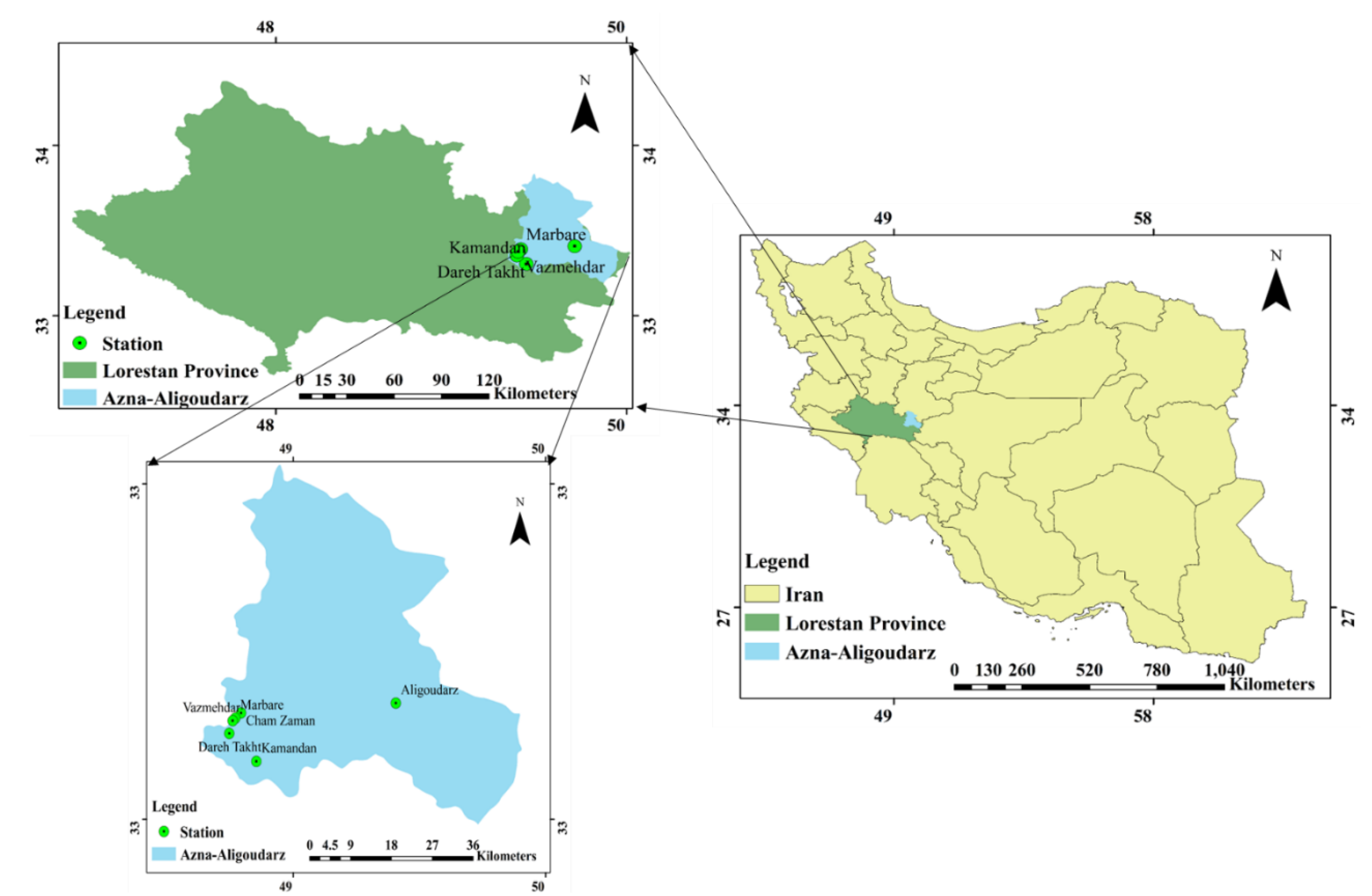
Figure 2.
(a) Monthly average precipitation distribution, (b) Monthly average temperature distribution in the period from 1993 to 2023.
Figure 2.
(a) Monthly average precipitation distribution, (b) Monthly average temperature distribution in the period from 1993 to 2023.
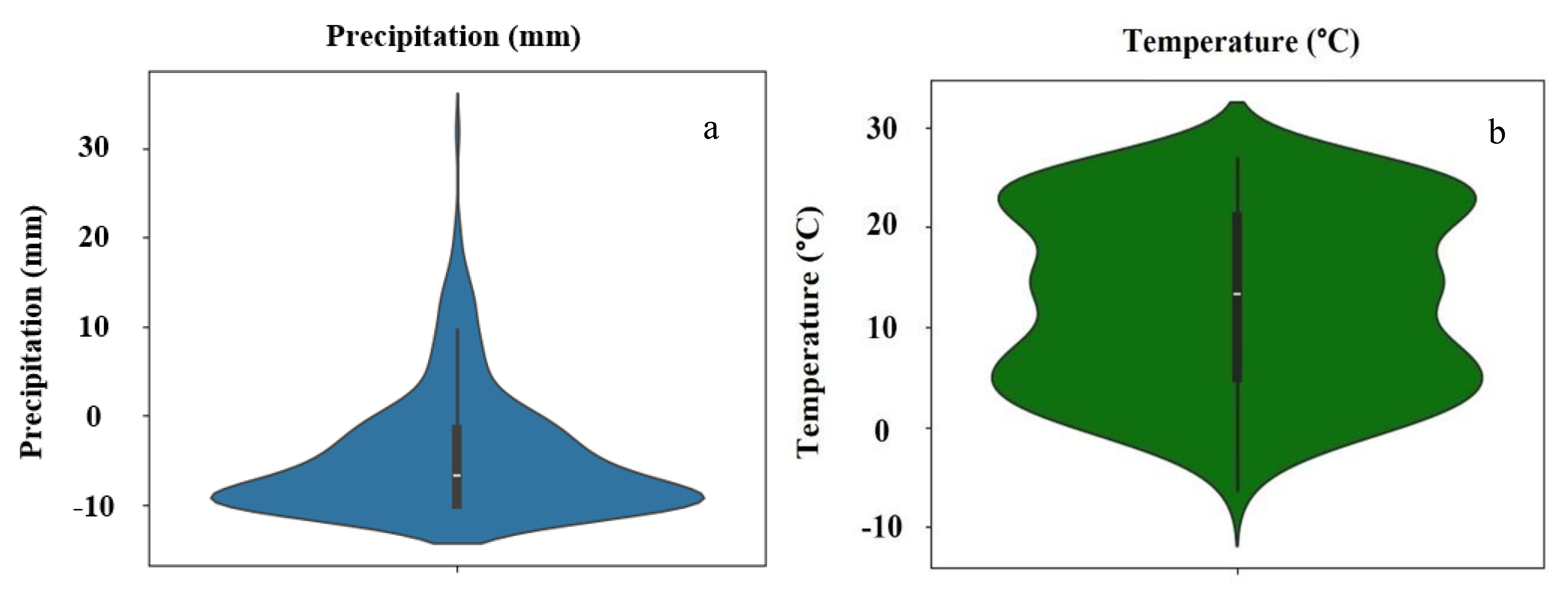
Figure 3.
Discharge distribution of hydrometric stations in the period from 1993 to 2023.
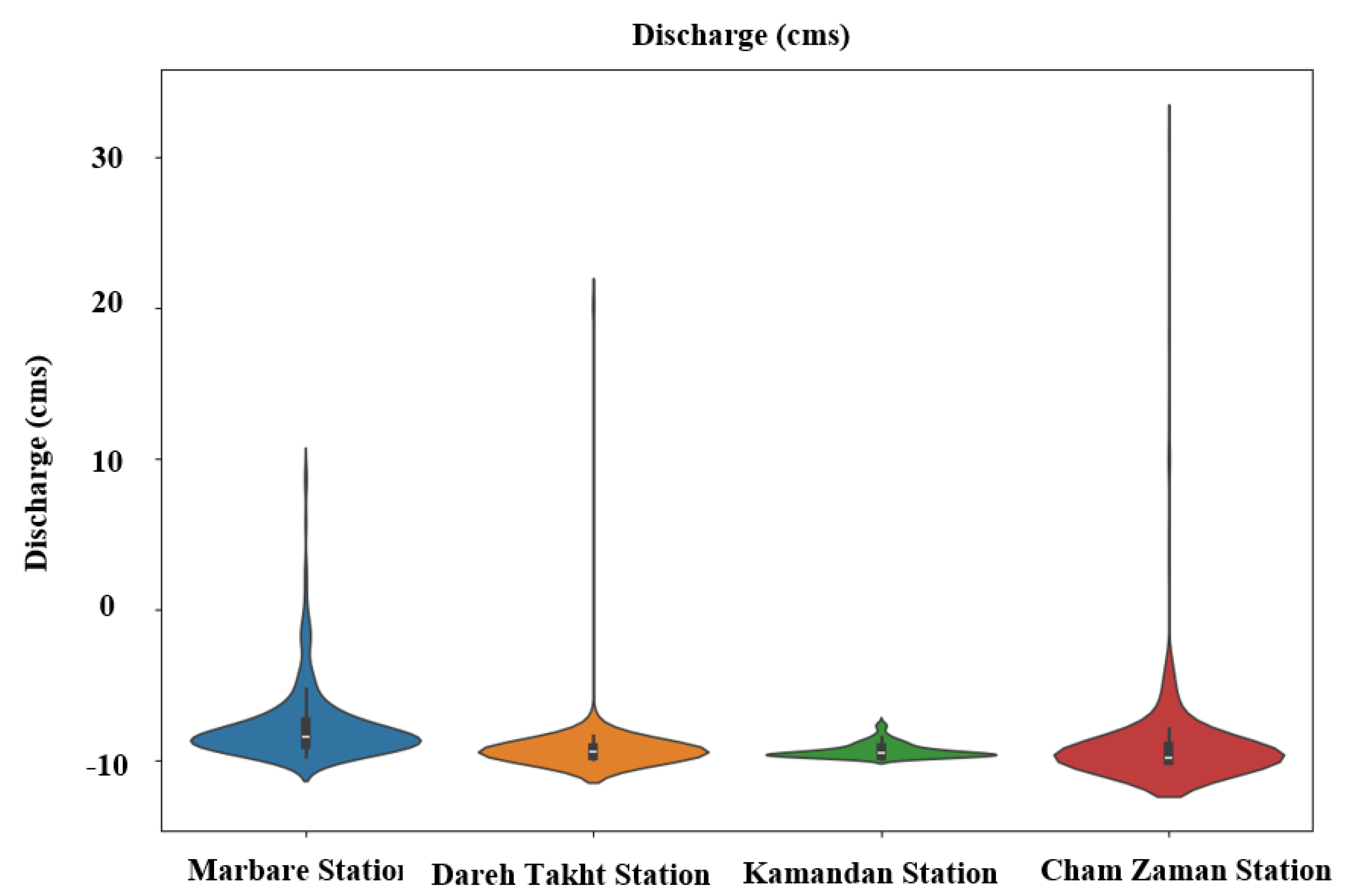
Figure 4.
Input maps of (a) digital elevation map, (b) Division of sub-basins.
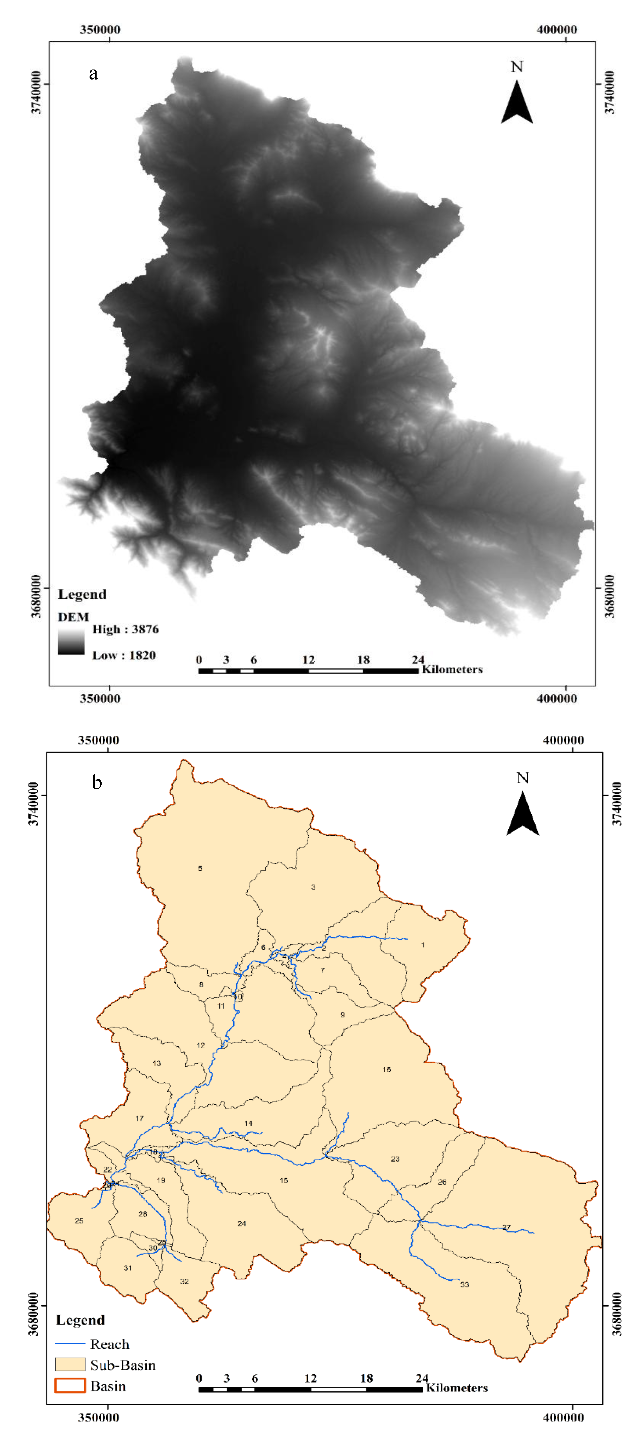
Figure 5.
Input maps of (a) Land use, (b) Soil class, (c) Slope of the study area.
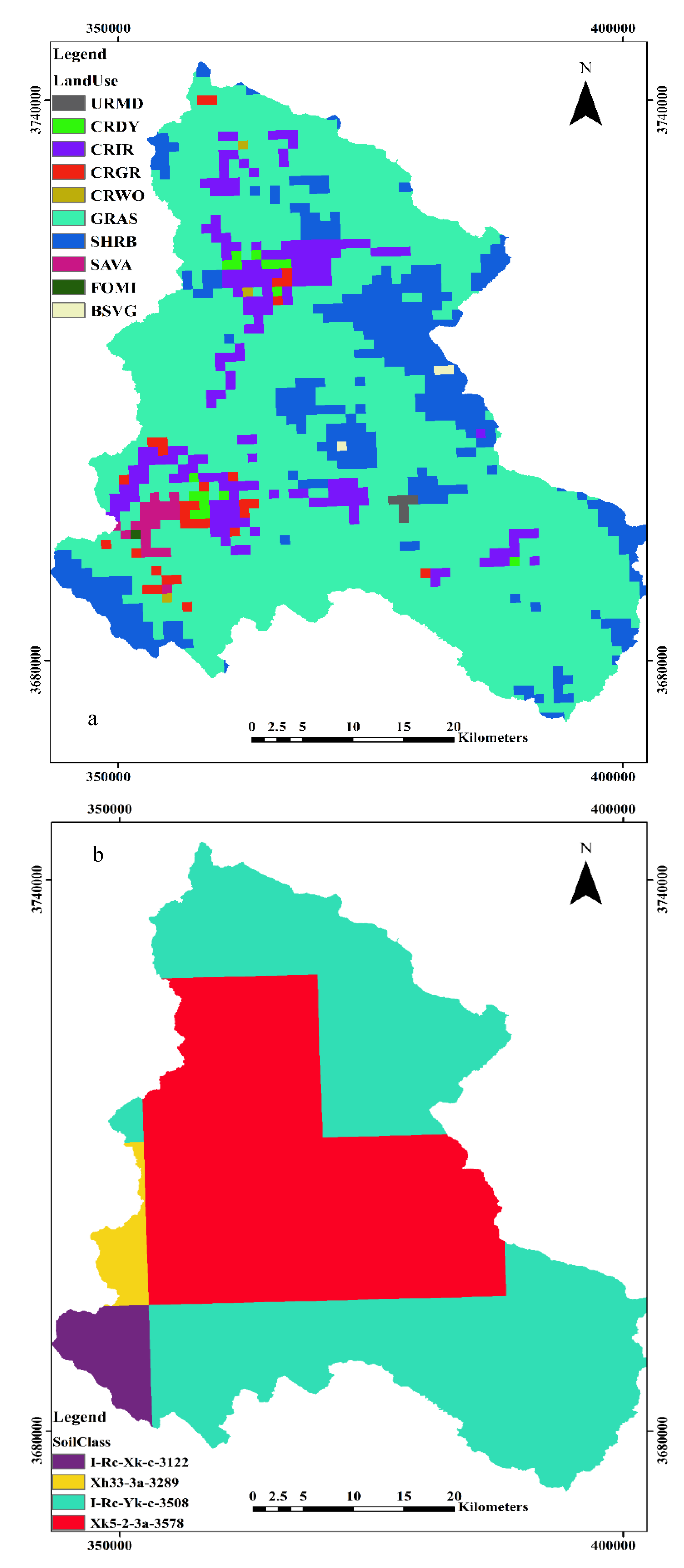
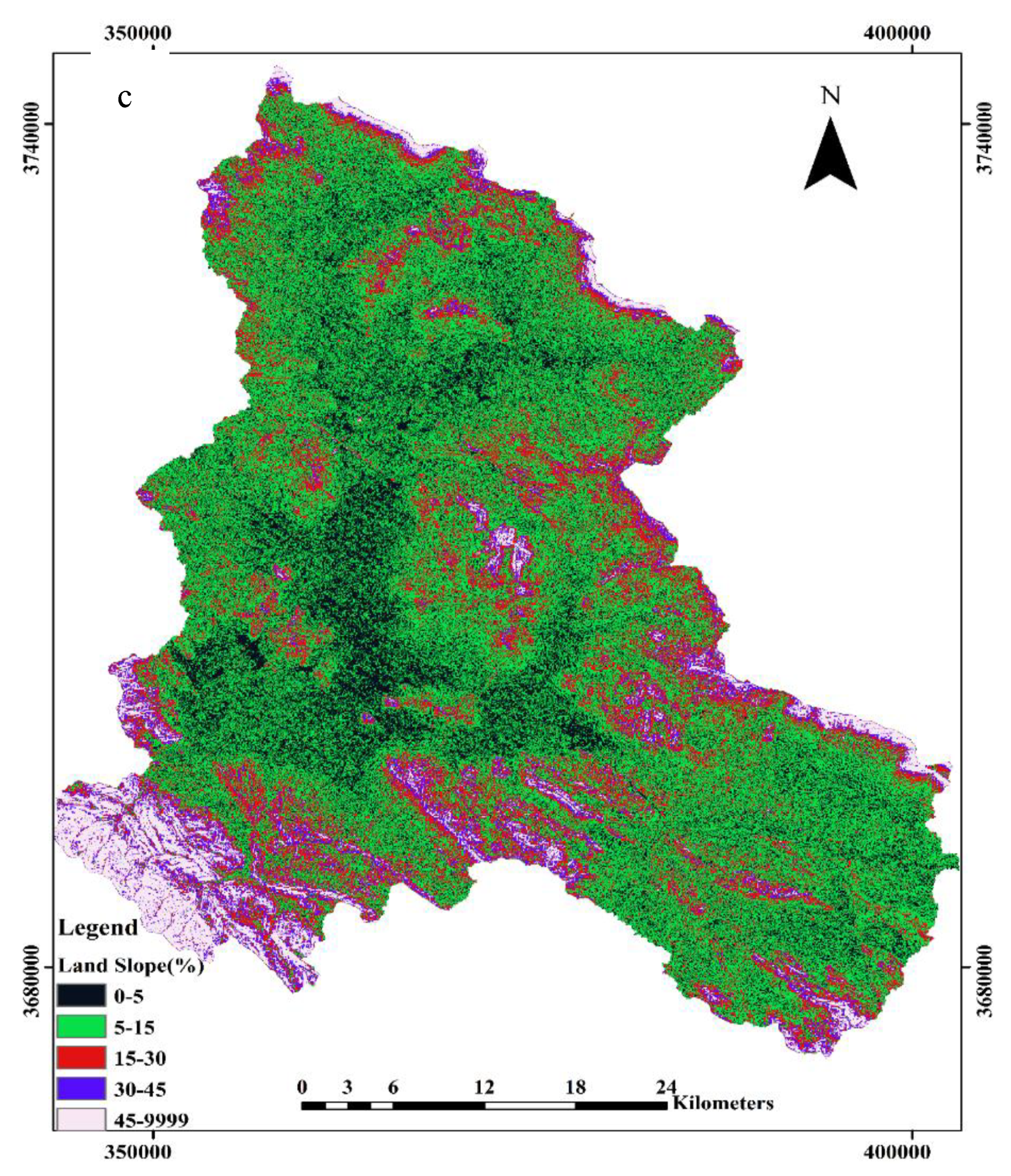
Figure 6.
Diagram of time changes of simulated runoff and observed runoff in the study area.
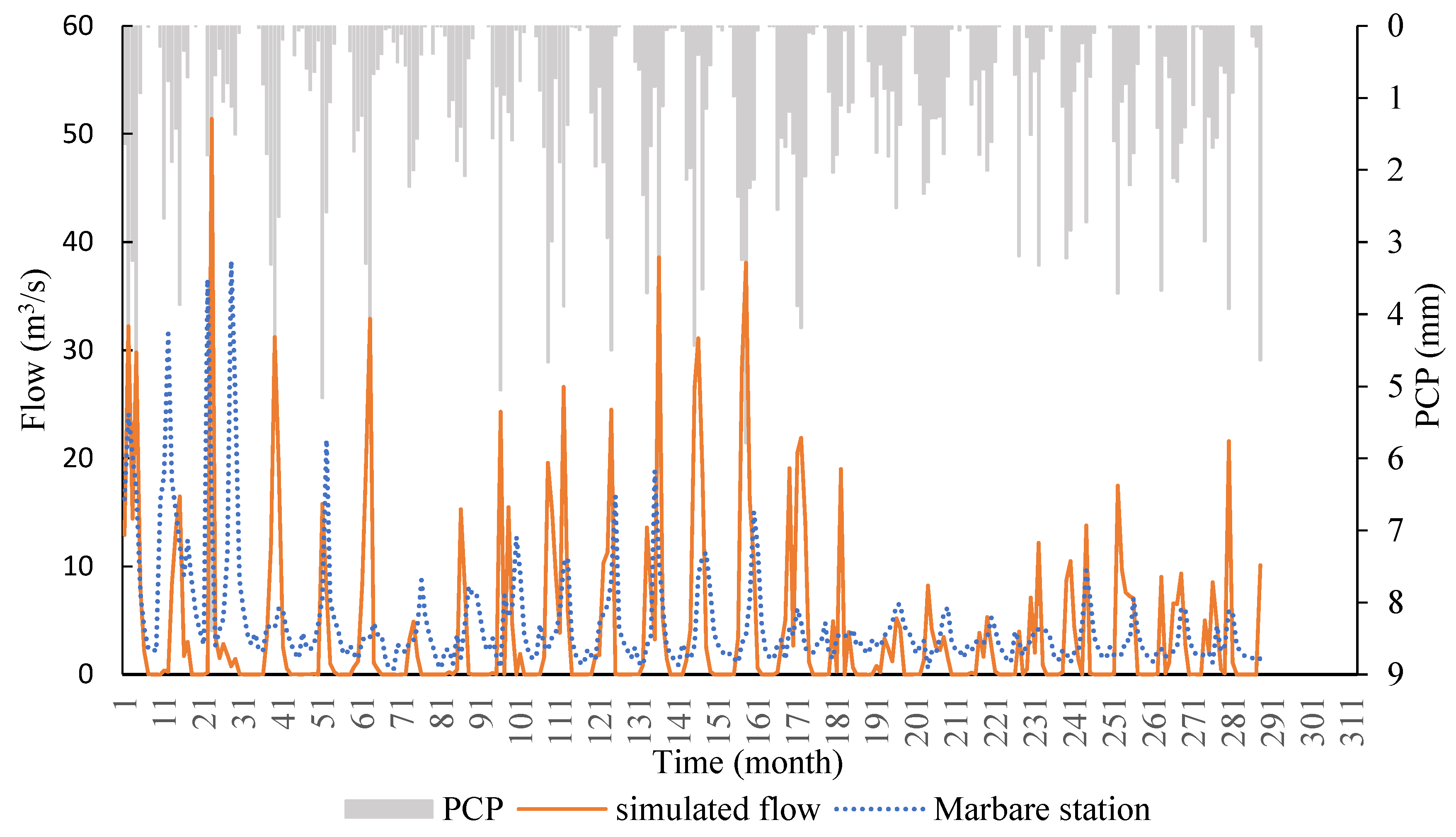
Figure 7.
Comparative analysis between simulated discharge and observed values for four stations in the studied area.
Figure 7.
Comparative analysis between simulated discharge and observed values for four stations in the studied area.
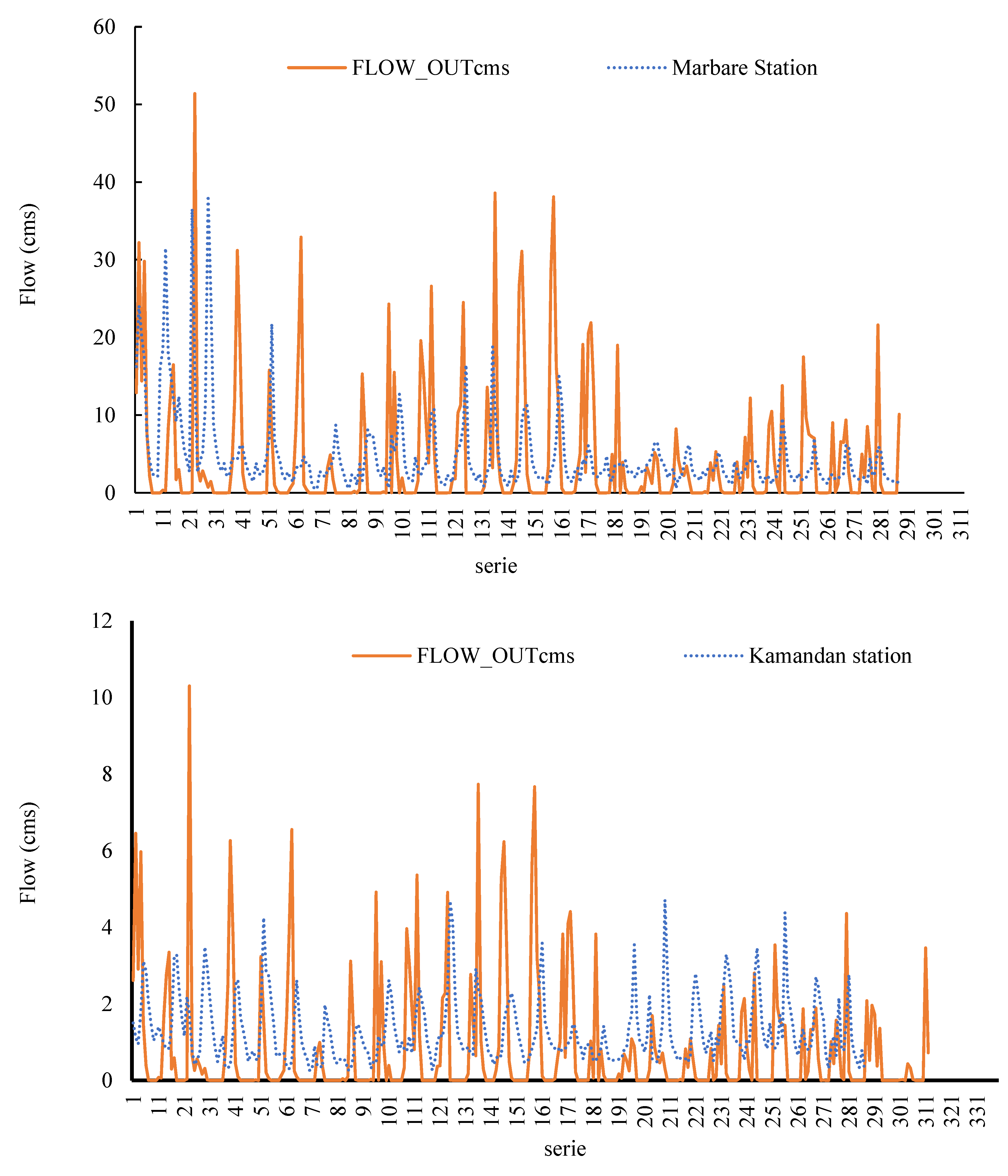
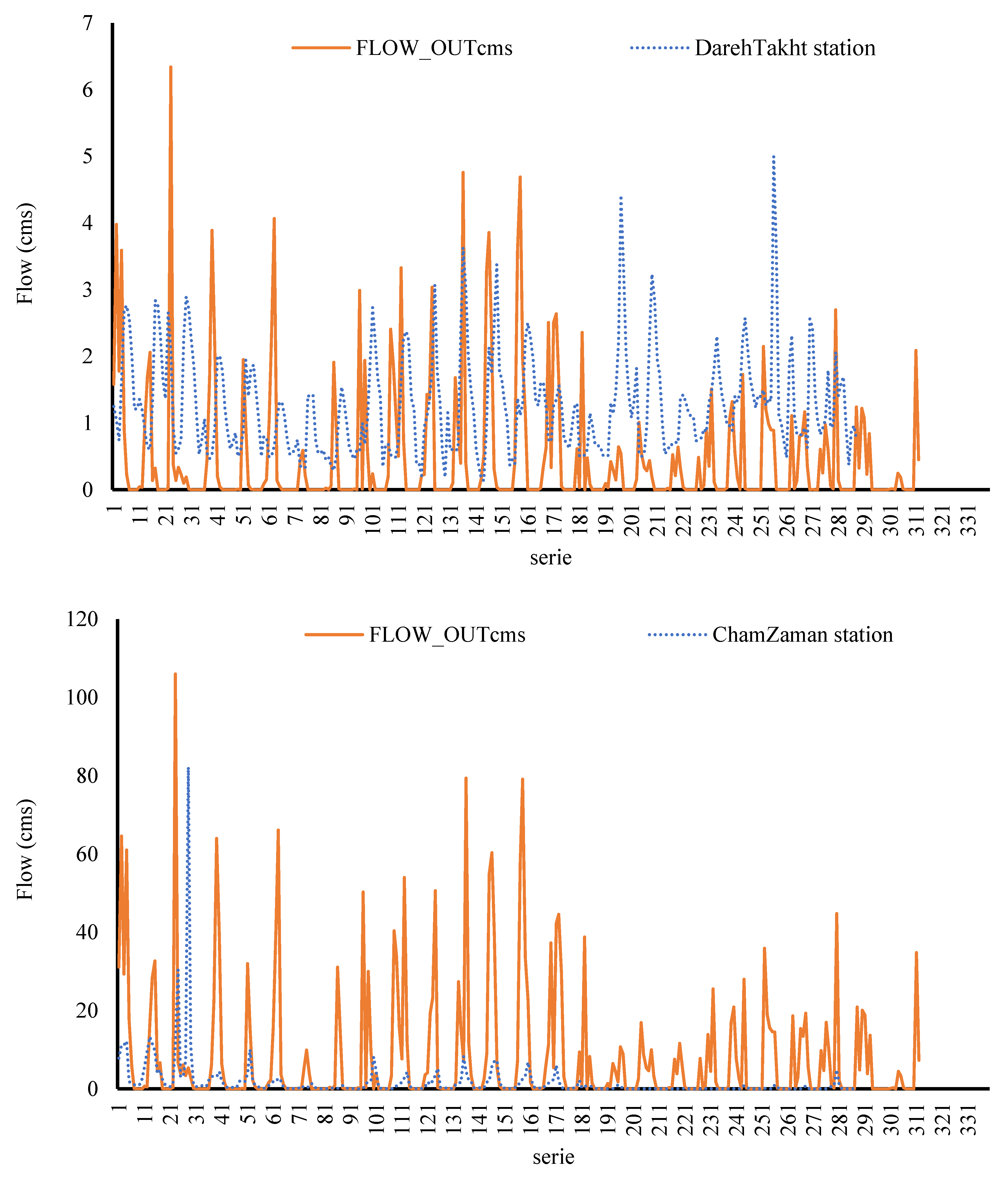
Figure 8.
Variations in observed and simulated runoff the studied area within time span 1993-2009 using full dataset.
Figure 8.
Variations in observed and simulated runoff the studied area within time span 1993-2009 using full dataset.
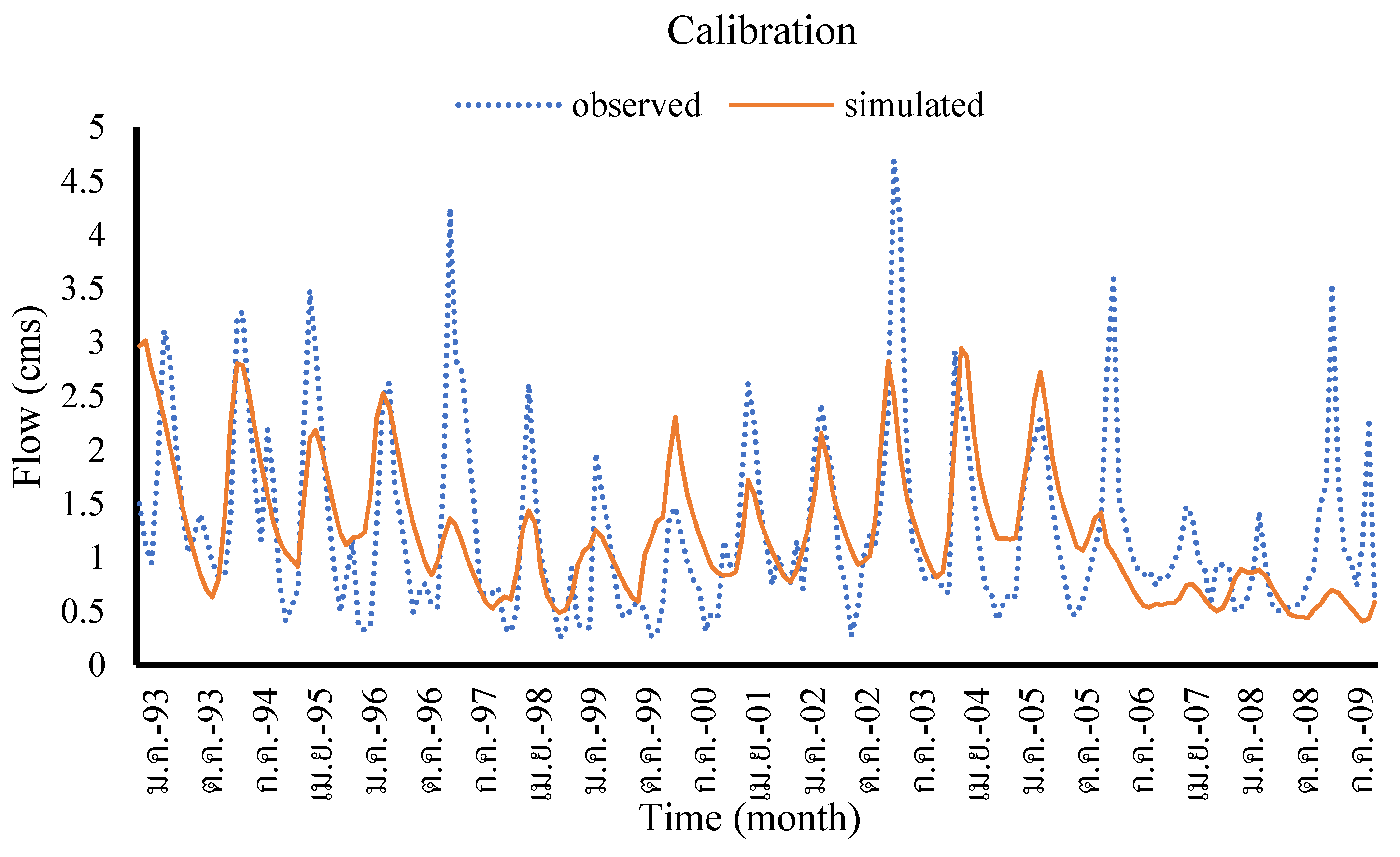
Figure 9.
Variations in observed precipitation, temperature and discharge at Marbare station (a), and in simulated discharge (b).
Figure 9.
Variations in observed precipitation, temperature and discharge at Marbare station (a), and in simulated discharge (b).
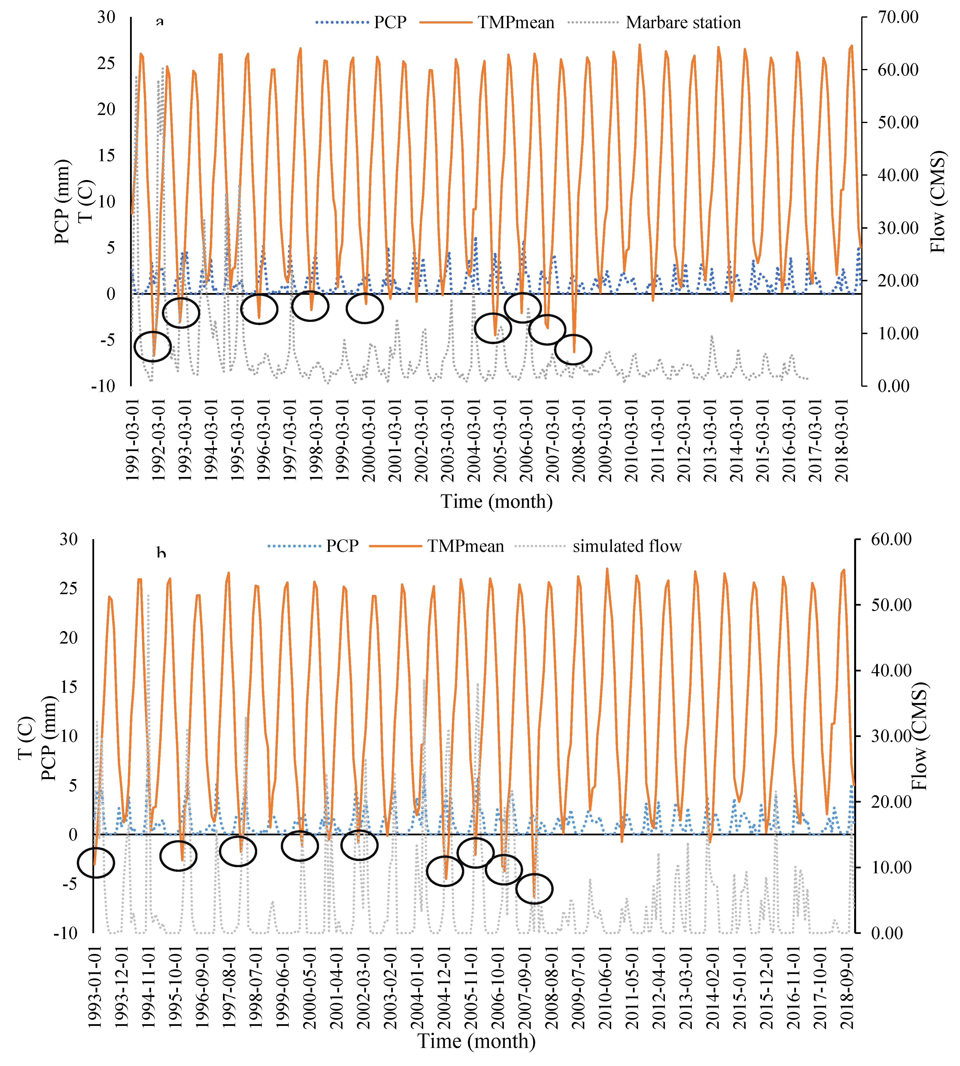
Figure 10.
Comparison of observed and simulated values of flow at (a) calibration, (b) validation phases.
Figure 10.
Comparison of observed and simulated values of flow at (a) calibration, (b) validation phases.
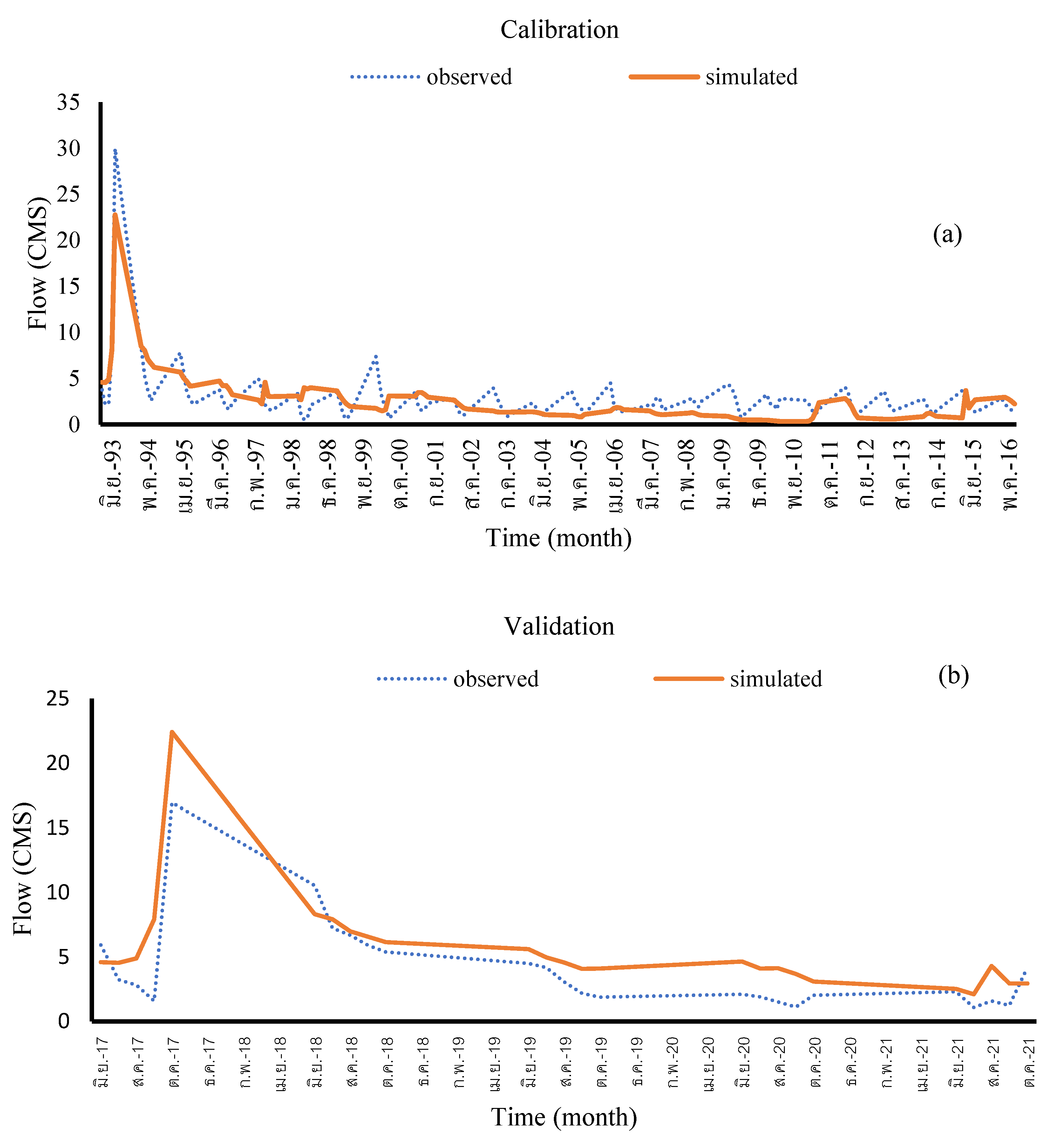
Figure 11.
Graphical depict of snowpack values (a) and its distribution (b) at the outlet station for both Scenarios A and B.
Figure 11.
Graphical depict of snowpack values (a) and its distribution (b) at the outlet station for both Scenarios A and B.
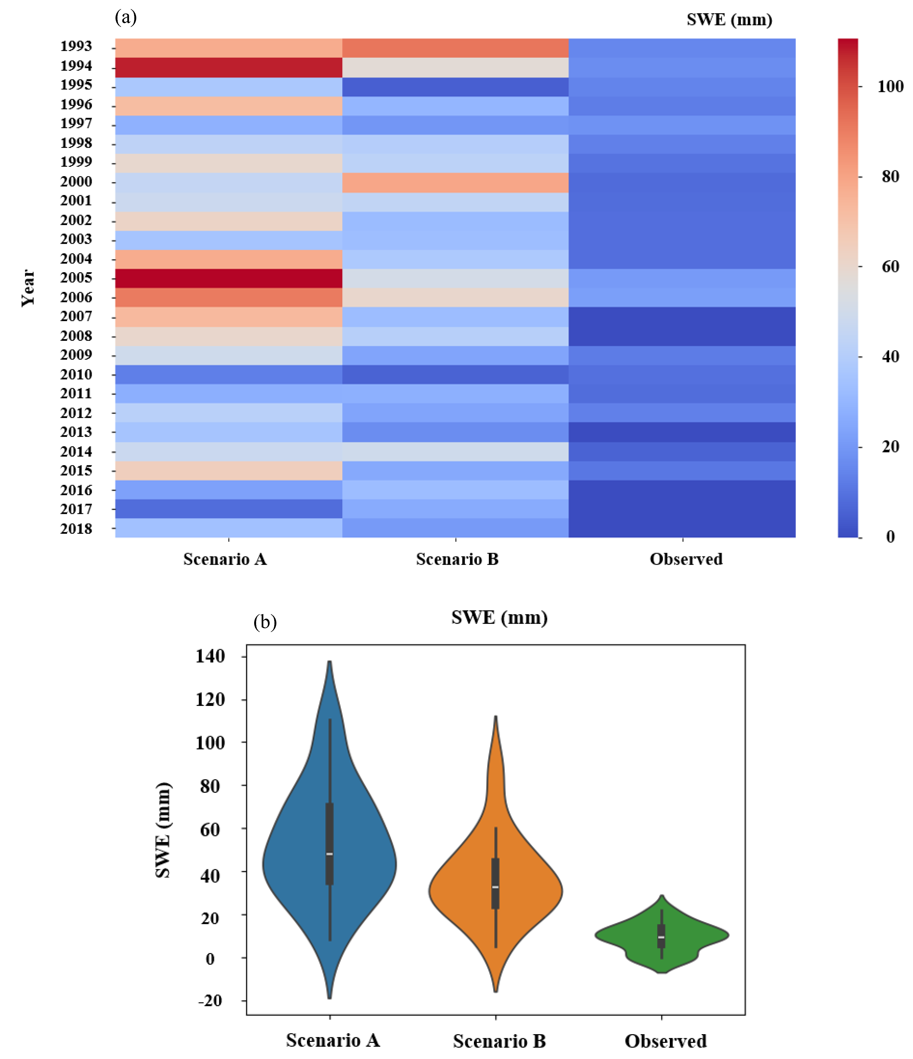
Figure 12.
Graphical depict of snowmelt parameters (a) Snowmelt distribution (b at the outlet station for both Scenarios A and B.
Figure 12.
Graphical depict of snowmelt parameters (a) Snowmelt distribution (b at the outlet station for both Scenarios A and B.
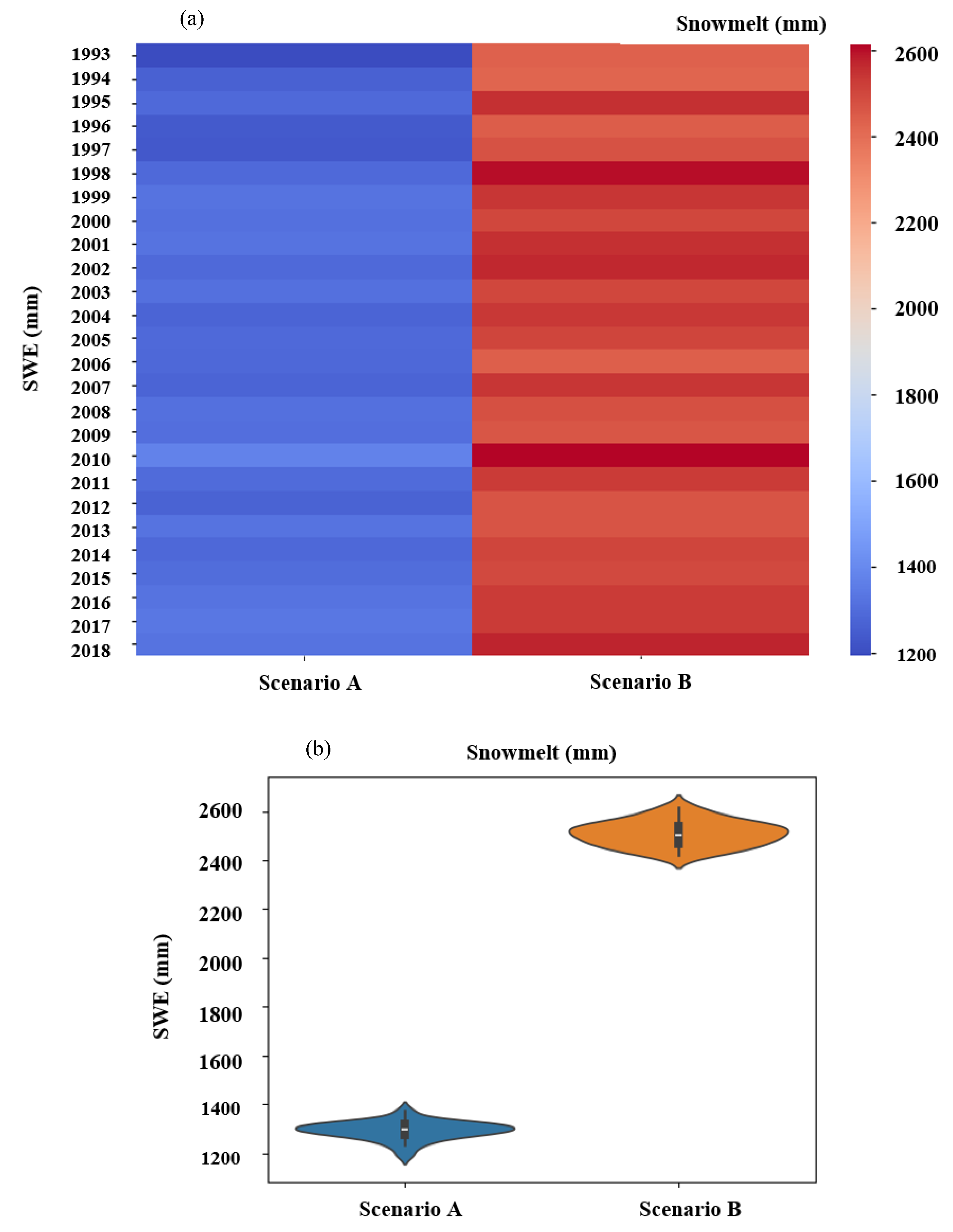
Table 1.
Climatic information of a Aligoudarz synoptic station.
| Station | Frost (day) | Sun. (hour) | Evap. (mm/day) | Max. rainfall (24 hr) | Rainfal (mm) | Avg. humidity (٪) | Avg. Temp. (°C) | Climatic division |
|---|---|---|---|---|---|---|---|---|
| Aligoudarz | 99 | 2749.7 | 2048.2 | 70.4 | 387.3 | 40 | 12.4 | Semi-humid Mild summer Very cold winter |
Table 2.
Characteristics of the hydrometry stations located in studied area.
| Station | Station’s type | Establishment | Altitude(m) | Latitude | Longitude |
|---|---|---|---|---|---|
| Aligoudarz | Synoptic | 1985 | 1980 | °33 ’24 | °49 ’42 |
| Kamandan | Rain Gauge Hydrometry | 1967 | 2050 | “14’18 °33 | °49’25“36 |
| Dareh Takht | Rain Gauge Hydrometry | 1955 | 1940 | “14’21 °33 | °49’22 “23 |
| Marbare | Hydrometry | 1958 | 1820 | “52’22 °33 | °49’24 “6 |
| ChamZaman | Hydrometry | 1961 | 1870 | “36’23 °33 | °49’23 “27 |
| Vazmehdar | Snow Gauge | 1974 | 1912 | “35’22 °33 | °49’22 “47 |
Table 3.
Land use coverage in studied area.
| Land use type | Abbreviations | Area (%) | Area (Km2) |
|---|---|---|---|
| Grassland | GRAS | 72.5 | 1588.5 |
| Shrubland | SHRB | 15.7 | 343.8 |
| Irrigated cropland and pasture | CRIR | 8.2 | 179.5 |
| Cropland/grassland mosaic | CRGR | 1.3 | 30.1 |
| Cropland/woodland mosaic | CRWO | 0.1 | 2.9 |
| Baren or sparsely vegetated | BSVG | 0.1 | 2.9 |
| Savanna | SAVA | 0.9 | 19.8 |
| Dryland cropland and pasture | CRDY | 0.7 | 15.5 |
| Residential-medium density | URMD | 0.2 | 4.8 |
| Mixed forest | FOMI | 0.04 | 0.9 |
Table 4.
Soil classes in studied area.
| Soil texture type | Abbreviations | Area (%) | Area (Km2) | |
|---|---|---|---|---|
| Loam | I-Rc-Yk-c-3508 | 53.813 | 1178.3 | |
| Clay_loam | Xk5-2-3a-3578 | 40.3 | 881.8 | |
| Loam | I-Rc-Xk-c-3122 | 3.8 | 82.5 | |
| Clay_loam | Xh33-3a-3289 | 2.1 | 46.3 |
Table 5.
Effective parameters and their optimal values in model calibration.
| Parameter | Opt. | Max. Min. | Var. type | Description | |
|---|---|---|---|---|---|
| CN2.mgt | -0.49 | -0.48 | -0.5 | Multiply | SCS runoff curve number (-) |
| ALPHA_BF.gw | 0 | 0.01 | 0 | Replace | Base flow alpha factor (1/days) |
| GW_DELAY.gw | 306.1 | 310.14 | 305.68 | Replace | Groundwater delay time (days) |
| GWQMN.gw | 0.92 | 0.95 | 0.91 | Replace | Threshold depth in shallow aquifer for return flow (mm) |
| GW_REVAP.gw | 0.15 | 0.15 | 0.15 | Replace | Coefficient for groundwater revap (days) |
| CH_K2.rte | 103.56 | 103.64 | 103.49 | Replace | Effective hydraulic conductivity in main channel alluvium |
| SOL_AWC(..).sol | 0.88 | 0.89 | 0.88 | Multiply | Available water capacity of the soil layer (mmH2O/mm soil) |
| SOL_K(..).sol | 0.26 | 0.26 | 0.26 | Multiply | Saturated hydraulic conductivity (mm/hr) |
| REVAPMN.gw | 1.02 | 1.02 | 1.02 | Replace | Threshold depth in shallow aquifer for revap/percolation (mm) |
| OV_N.hru | -0.01 | -0.01 | -0.01 | Multiply | Manning’s “n” value for overland flow (-) |
| SLSUBBSN.hru | 0.21 | 0.21 | 0.21 | Multiply | Average slope length (m) |
| PLAPS.sub | -13.34 | -13.34 | -13.34 | Replace | Precipitation laps rate |
| SURLAG.bsn | 14.75 | 14.75 | 14.75 | Replace | Surface runoff lag time |
| TLAPS.sub | -9.72 | -9.72 | -9.72 | Replace | Temperature laps rate |
| SFTMP.bsn | 10.47 | 10.47 | 10.46 | Replace | Snowfall temperature |
| SMTMP.bsn | -9.89 | -9.89 | -9.89 | Replace | Snowmelt base temperature |
| SMFMX.bsn | 4.58 | 4.59 | 4.58 | Replace | Maximum melt rate for snow during year |
| SMFMN.bsn | 0.88 | 0.88 | 0.87 | Multiply | Minimum melt rate for snow during the year |
| SNOEB(..).sub | 310.65 | 310.66 | 310.64 | Replace | Initial snow water content in elevation bands |
| SNOCOVMX.bsn | -35.24 | -35.23 | -35.45 | Replace | Snow water content that corresponds to 100% snow cover |
| ALPHA_BNK.rte | 0.03 | 0.03 | 0.03 | Replace | Baseflow alpha factor for bank storage (day) |
| SOL_BD(..).sol | -0.52 | -0.51 | -0.52 | Multiply | Moist bulk density |
Disclaimer/Publisher’s Note: The statements, opinions and data contained in all publications are solely those of the individual author(s) and contributor(s) and not of MDPI and/or the editor(s). MDPI and/or the editor(s) disclaim responsibility for any injury to people or property resulting from any ideas, methods, instructions or products referred to in the content. |
© 2025 by the authors. Licensee MDPI, Basel, Switzerland. This article is an open access article distributed under the terms and conditions of the Creative Commons Attribution (CC BY) license (http://creativecommons.org/licenses/by/4.0/).
Copyright: This open access article is published under a Creative Commons CC BY 4.0 license, which permit the free download, distribution, and reuse, provided that the author and preprint are cited in any reuse.


