
Submitted:
22 September 2025
Posted:
23 September 2025
You are already at the latest version
Abstract
The Virial theorem has been applied with considerable success in various fields of natural sciences. This proposal shows its extension by applying it to discrete data series. This application will be called the Virial theorem extension and can be applied to the numerical solution of nonlinear dynamic systems represented by difference equations, such as logistic, discubic and random number generators. differential equations like the nonlinear double pendulum and series of pseudorandom numbers and its reciprocals. The results obtained show that the proposal characterizes and distinguishes different types of behavior from the series under study. It also shows great sensitivity to the evolution of the series, even anticipating critical points. The proposed method to construct the discrete Virial extension does not require the existence of a Hamiltonian, which allows its application to series obtained experimentally. For pseudorandom number series, the extension reveals a consistent, quasi-specular behavior between its kinetic and potential factors, suggesting an underlying structural property. From a general point of view, this research shows a series of properties that can be reinterpreted in light of the discrete Virial coefficient, providing a novel and versatile tool given its minimal applicability requirements.
Keywords:
Virial theorem
; Time Series Analysis
; discrete systems
; Chaos Theory
; Feigenbaum Diagram
; Dynamical Systems
1. Introduction
The Virial theorem has been widely used in the physical sciences; for an introduction, see [1], and for a variety of applications, can be consulted, for example [2,3,4,5,6,7,8,9] among many others. In general, its use is related to the equivalence of kinetic and potential energy. In its original version, the variables have a continuous evolution, but when digital processing is used, discretization is necessarily required. The solution of the non-linear equations and the evolution of the experimental variables are expressed in terms of discrete data sequences. In this research, an extended formalism of the Virial theorem is applied to discrete data series using the numerical evaluation of the derivatives through the centered approximation of the derivative of order two [10,11]. The result when the generalization of the Virial theorem is applied to the series generated by the solution of differential equations is similar to that already known for the continuous theoretical evolution of the variables. This extension to discrete variables shows how convergence to expected values can provide information about the characteristics of the series and about the possible operational origin of the data. For this reason, the logistic, discubic, Sin, and gaussian map equations are studied in detail. Although the origin of the Virial theorem is directly related to the kinetic and potential energy of a physical system, it was exposed here that it is possible to become independent of these concepts. However, the mathematical properties are still present as a pseudo-conservation of energy. Finally, this approach expands the results of previous works on discrete Virial theorems for symplectic maps [12] by removing the requirement of a known Hamiltonian, thus broadening its applicability to any time series, including those of experimental origin. However, this computation allows one to determine how close the origin of the series is to a Hamiltonian symplectic manifold. Some potential applications and limitations of this concept extension were explored. The present work is organized as follows: in the Section 2 is introduced the general (continuous) treatment of the Virial theorem without taking into account the nature of the system that produces the data series, in the Section 3 the extension of the formalism for the discrete case is introduced, in Section 4 examples of the application of the discrete Virial formalism are analyzed in detail, Section 5 is devoted to the study the information provided by the extension of the Virial theorem to discrete chaotic iterative maps, in Section 6 the use of the new proposal are applied to measured data series, the global results of the research are included in Section 7, and finally in Section 8 the concluding remarks of the work are presented.
2. General Continuous Treatment
Consider the Virial theorem in the case of a continuous function . In this section, the Virial theorem is reformulated without considering a physical system, that is, using only mathematical considerations without reference to kinetic or potential energies. Let t be a time variable. Assume that the first and second time derivatives of exist and that , and are bounded. The Virial expression can be formulated (analogously to the derivation of the Virial theorem of mechanics) as a new function of t given by:
differentiating with respect to t,
Then the time average it taken over a sufficiently large time interval :
Applying the time average to Equation (2):
The left-hand side of promedios Equation (4) becomes:
Since and are bounded, is also bounded. Therefore,
Thus, in this way, the continuous Virial theorem of the following form is obtained:
The result of Equation (6) is applicable to analytical solutions of certain systems, given the initial assumptions about and its derivatives. From Equation (6), it is possible to define the Virial coefficient C:
which approaches 1 as under these assumptions.
As can be seen from this brief deduction, the only assumptions are that the function is bounded and at least twice differentiable, which allows to obtain the expression of C. In the next section, this reasoning will be extended to discrete data series, regardless of their origin.
3. New Formalism: Discrete Virial Formalism Extension
In this section, the Virial formalism for discrete series, such as those arising from numerical solutions of difference or differential equations or experimental measurements is introduced.
A numerical series represents values at discrete points i, where i is typically an integer index, for example ranging from 1 to N. The interval between points is assumed constant, denoted by h. it is assumed that the underlying process generating has bounded behavior analogous to the continuous case.
For the numerical evaluation of derivatives, the second-order centered difference approximation [10] is used:
The average over a series of length N is defined as:
Analogous to the continuous case, it can be considered the discrete version of , which is . Examining in detail the structure related to its derivative and Equation (2) averaged over a data series of N terms, which gives:
Here, represents the average change in over the interval . Similarly to the continuous case, for bounded series, the average change tends to zero for large N:
The important point is that Equation (10) (with the left hand side approaching zero) is an extension to discrete series of Equation (4). Its validity depends on and the suitability of the derivative approximations. If originates from a process well-described by a differential equation satisfying the initial assumptions, then the discrete Virial relation holds approximately.
3.1. Kinetic and Potential Factors
Following the terminology of the original Virial theorem, it can be defined the discrete kinetic (K) and potential (P) components for the Virial coefficient C:
The discrete form for the Virial coefficient, in terms of the and is given by:
For systems where the continuous Virial theorem holds (), it is expect as , provided h is sufficiently small relative to the variations of f.
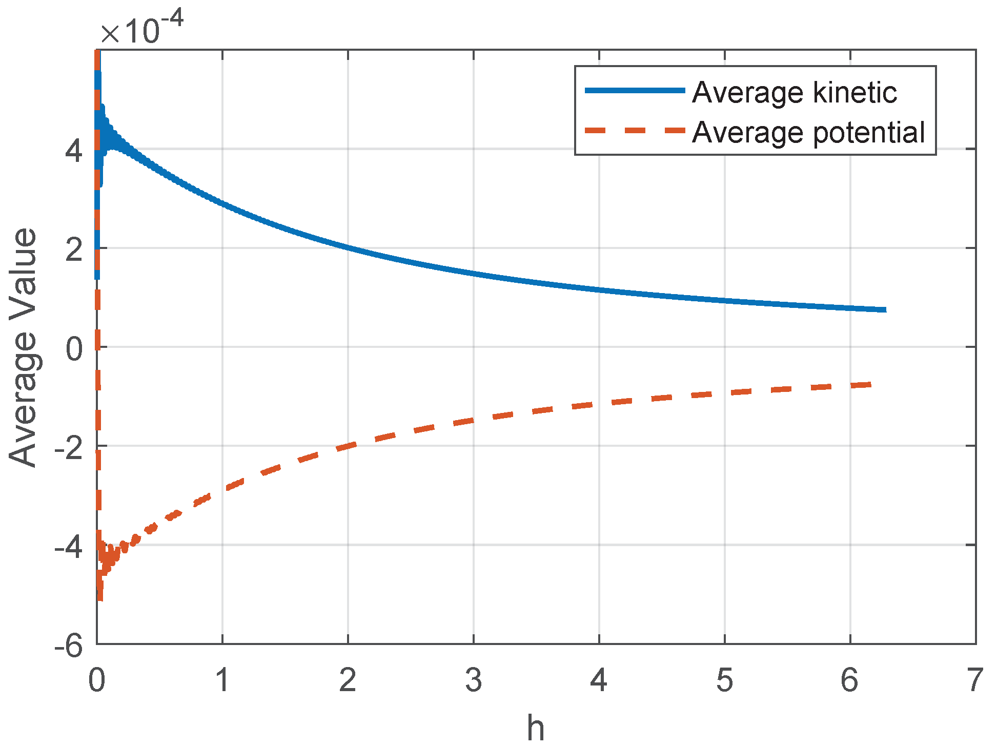
Figure 1.
Mirrored evolution of the kinetic factor and the potential factor of the evolution of the double pendulum.
Figure 1.
Mirrored evolution of the kinetic factor and the potential factor of the evolution of the double pendulum.
4. Examples and Detailed Analysis
4.1. Use in Chaotic Differential Equations
4.1.1. Double Pendulum
As already mentioned, for series generated as solutions of differential equations, the relation Equation (10) (with LHS→0) is approximately fulfilled and therefore .
A good example is the double pendulum. For small angles [13], the system is non-linear and the evolution becomes much more complex. The convergence analysis was performed for a chaotic double pendulum with lengths and masses as follows: , , , ; settled for each of them, respectively; the gravity was taken as . It was analyzed with chaotic behavior characterized by the Lyapunov exponent with value , data series length of 10000 points, and time step .
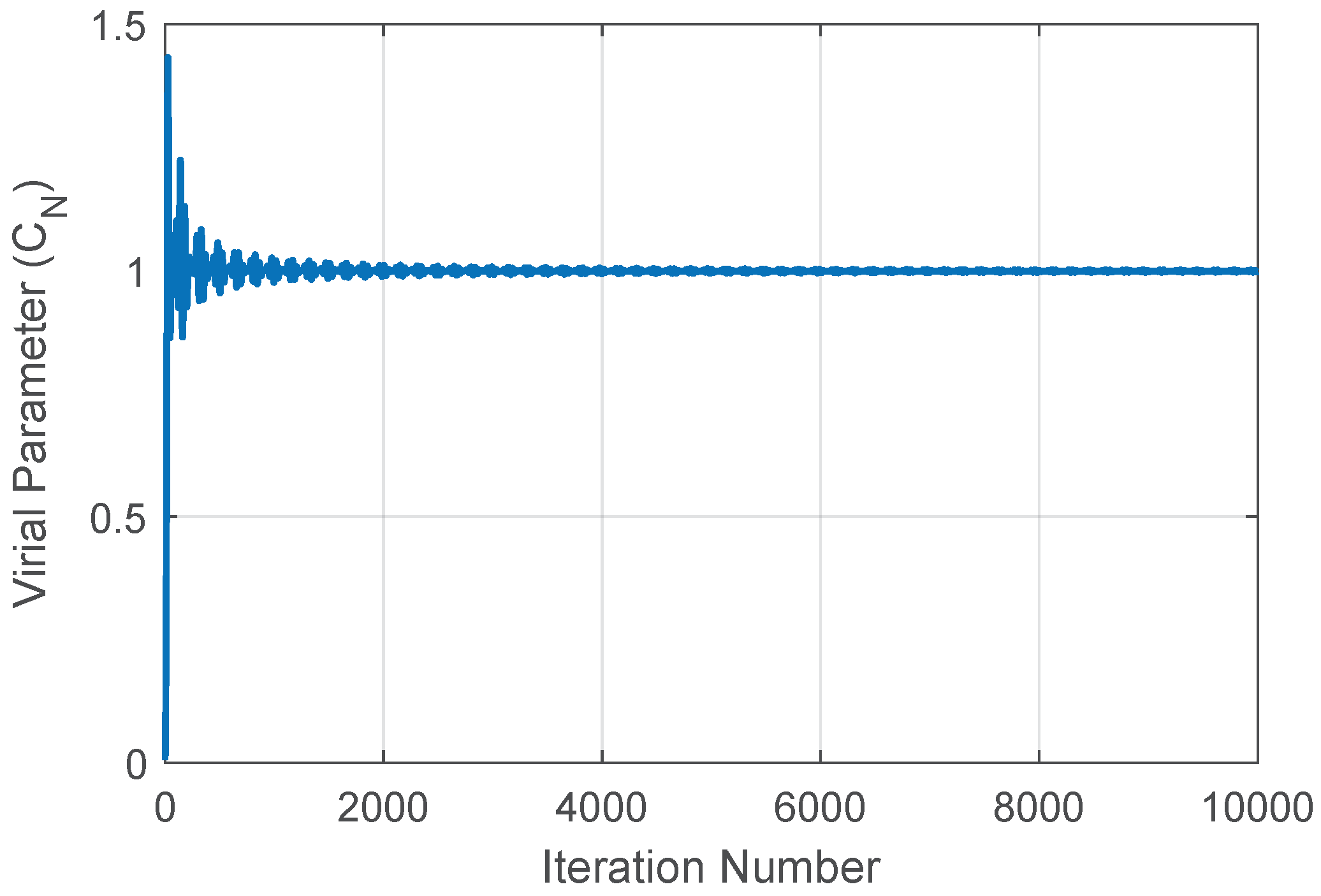
Figure 2.
Convergence of for the chaotic double pendulum.
When the potential and kinetic factors of the quotient that defines the discrete Virial coefficient behave as shown in Figure 1, it could be referred to as a virialization process, in which, once stabilized, they converge to a constant ratio value.
The convergence is shown in Figure 2 and the final result is ; the evolution corresponds to the mass () hanging from the other mass ().
4.2. Pseudorandom Numbers
Let a pseudorandom data series be generated by the Mersenne Twister algorithm [14], here the step , in such a way that the data values ranging between 0 and 1.
The derivative approximations from Equation (8) are formally applied to the series, despite it being an intrinsically non-differentiable distribution. However, because the series is discontinuous, the assumptions underlying the continuous Virial theorem (i.e., the existence of bounded derivatives) are violated. Consequently, while the average change term, , still approaches zero for a large, bounded series, the resulting ratio is not expected to converge to 1.
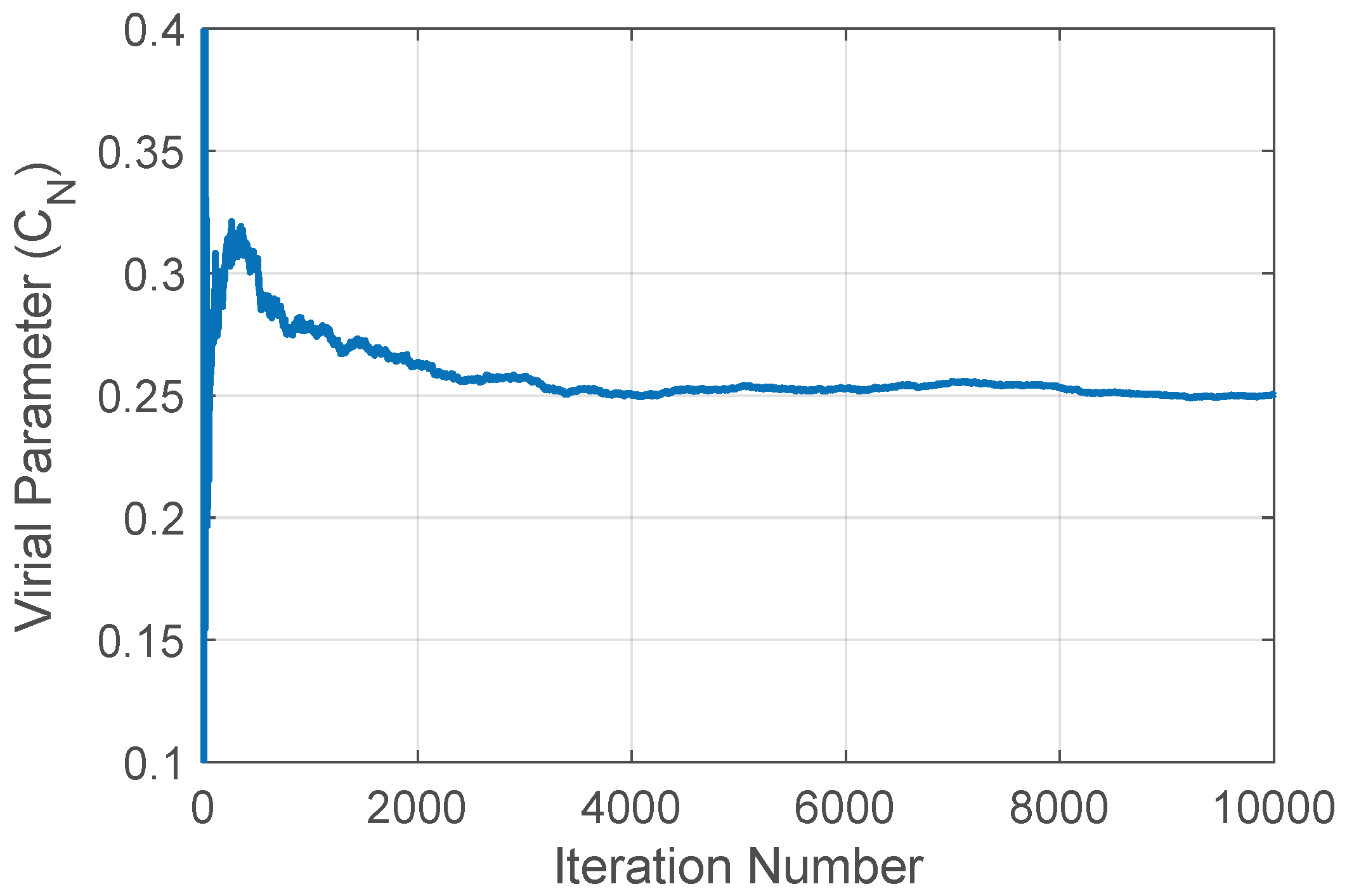
Instead, for a uniform pseudorandom distribution, the discrete Virial coefficient consistently converges to a different stable value. As can be seen in Figure 3, this value is approximately 0.25. This convergence implies that even within a stochastic series, the discrete kinetic () and potential () factors exhibit a consistent, quasi-specular behavior, leading to a stable ratio.
Figure 3.
Evolution of for Mersenne Twister pseudorandom numbers (0 to 1), . Converges to approximated 0.25.
Figure 3.
Evolution of for Mersenne Twister pseudorandom numbers (0 to 1), . Converges to approximated 0.25.
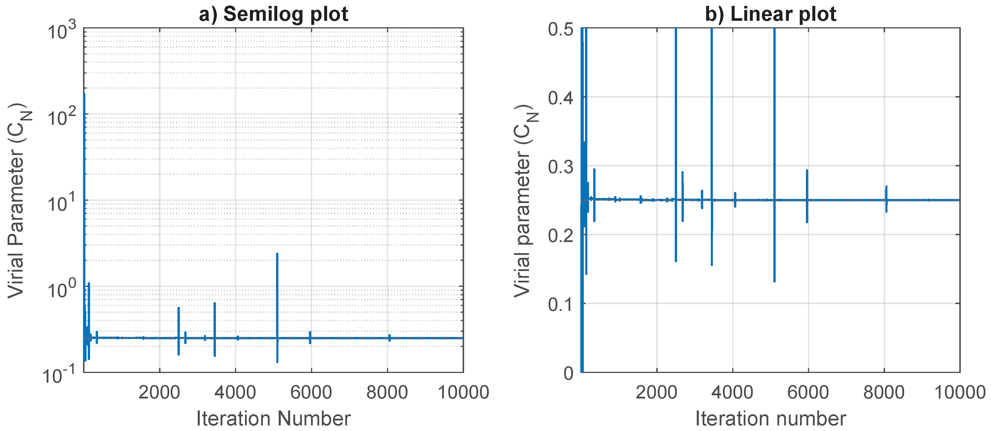
The pseudorandom series presented above can be redefined as it is the inverse, for , in such a way to get a quasi-bounded series. This is because some of the original numbers approach 0, and their inverse takes an unbounded jump. In Figure 4, the jumps that makes when the value of the pseudorandom number is very small (making the inverse very large). However, except for occasional jumps, remains at approximately 0.25 as the value of the data series increases.
Figure 4.
Evolution of for the inverse of pseudorandom numbers (). a) Semi-logarithmic axis showing large jumps when the pseudorandom number is near 0. b) Linear axis showing remaining close to 0.25 between jumps.
Figure 4.
Evolution of for the inverse of pseudorandom numbers (). a) Semi-logarithmic axis showing large jumps when the pseudorandom number is near 0. b) Linear axis showing remaining close to 0.25 between jumps.
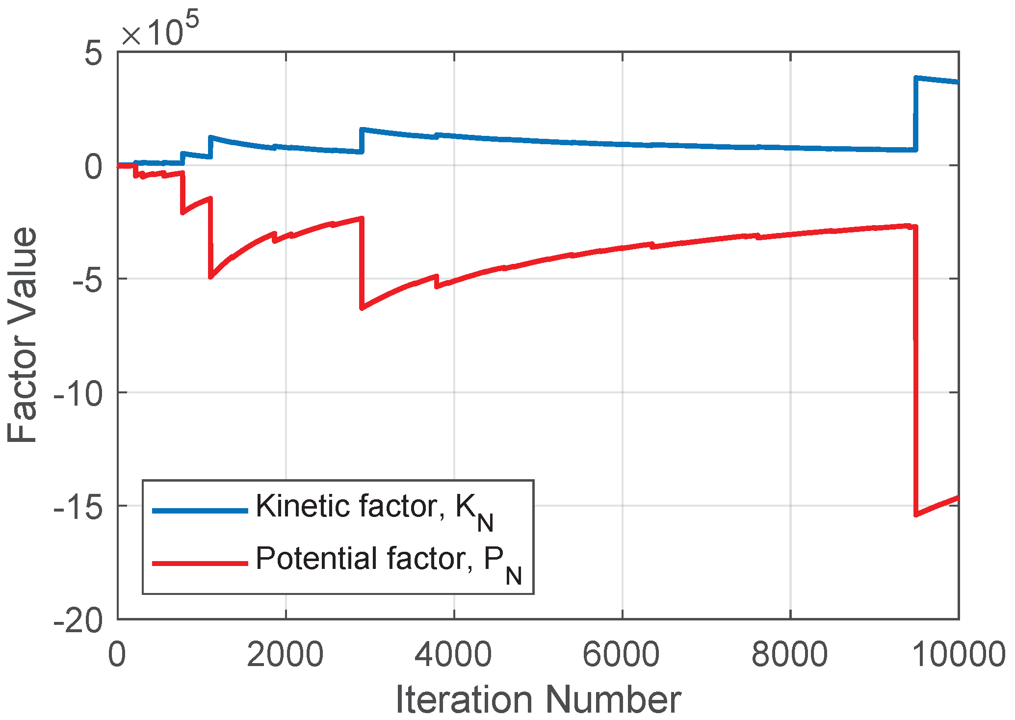
Revisiting the and factors for the pseudorandom number series, both factors look like they develop in a mirror image fashion, but with different scales; see Figure 5. Note that the potential factor is larger in magnitude than the kinetic factor. Any value that tends to be very large (such is the inverse of jumps) will reset the convergence of .
Figure 5.
Evolution of the iterative kinetic factor (top, blue) and potential factor (bottom, red) for the reciprocal of the pseudorandom series, showing quasi-reflection but different amplitudes.
Figure 5.
Evolution of the iterative kinetic factor (top, blue) and potential factor (bottom, red) for the reciprocal of the pseudorandom series, showing quasi-reflection but different amplitudes.
4.3. Use in Difference Equations
4.3.1. Logistic Equation
Now, let us see a very popular difference equation, the logistic equation [15,16]:
The behavior of this equation is very subtle; and will be only analyzed some peculiarities. As with pseudorandom numbers, the derivatives of are undefined in a continuous sense. However, the relation Equation (13) can be reused by defining the derivative as suggested in Equation (8) (with ).
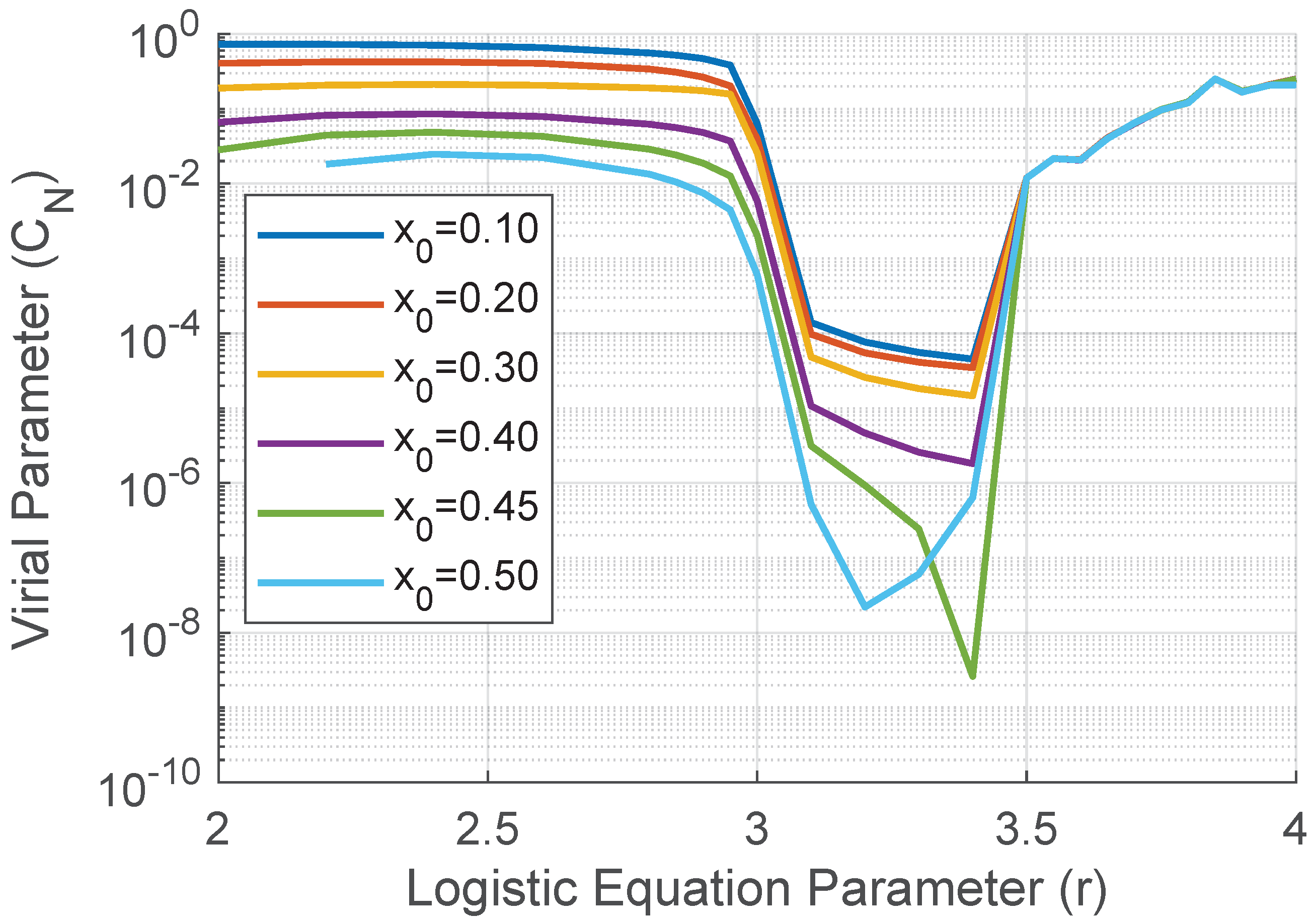
Analizing Figure 6 for the fixed point zone, the series stabilizes quickly and, therefore, the values of depend on the initial condition . When converging to the fixed point, all derivatives end up canceling; the numerator and denominator of the definition of decrease, although the quotient stabilizes in a limit that ultimately depends on the initial conditions.
For the bifurcation zone (period doubling), the definition of derivatives Equation (8) is not appropriate to capture the underlying dynamics. It can be seen that the alternating jump of values has a strong effect, because the first derivative term in the numerator of tends quickly to zero (e.g., for r=3.1 N=102; r=3.2 N=55; r=3.3 N=80; r=3.4 N=20000). In this range, the value of depends on the initial condition, because the iteration for which the effective derivative becomes zero depends in the same way. However, it is interesting to note that before reaching the first bifurcation, begins a variation that preannounces it. This is because the bifurcation is in progress and the first derivative term is in decline (Figure 6).
Figure 6.
Evolution of for the logistic equation with different initial conditions as parameter r varies. Note the drop before the first bifurcation around r=3.0 and dependence on initial conditions in the periodic regime.
Figure 6.
Evolution of for the logistic equation with different initial conditions as parameter r varies. Note the drop before the first bifurcation around r=3.0 and dependence on initial conditions in the periodic regime.
Beyond r=3.4 more bifurcations appear and depends on the initial conditions. For the chaotic zone of Pomeau-Manneville [17], the values of are independent of the initial conditions. Even for islands of stability within the chaos; although there are fixed points and bifurcations in these regions, they are so mixed that the dependence on the initial conditions is completely eliminated. The behavior on the islands of stability is similar, in such a way that the interest will be focused on the one with the longest duration (see Figure 7).
Figure 7.
Evolution of across an island of stability (period-3 window) in the chaotic zone of the logistic map (approximately from r=3.8250 to r=3.8570).
Figure 7.
Evolution of across an island of stability (period-3 window) in the chaotic zone of the logistic map (approximately from r=3.8250 to r=3.8570).
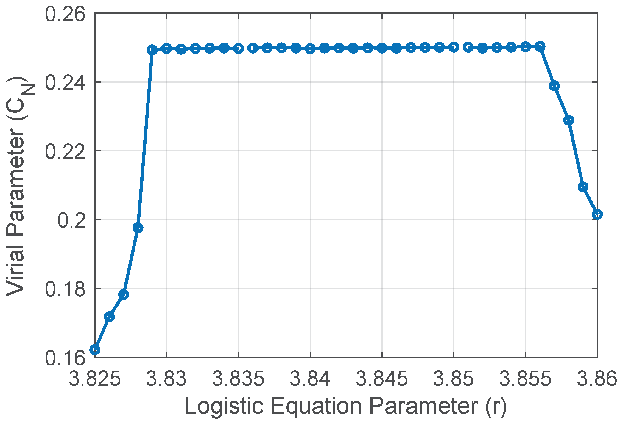
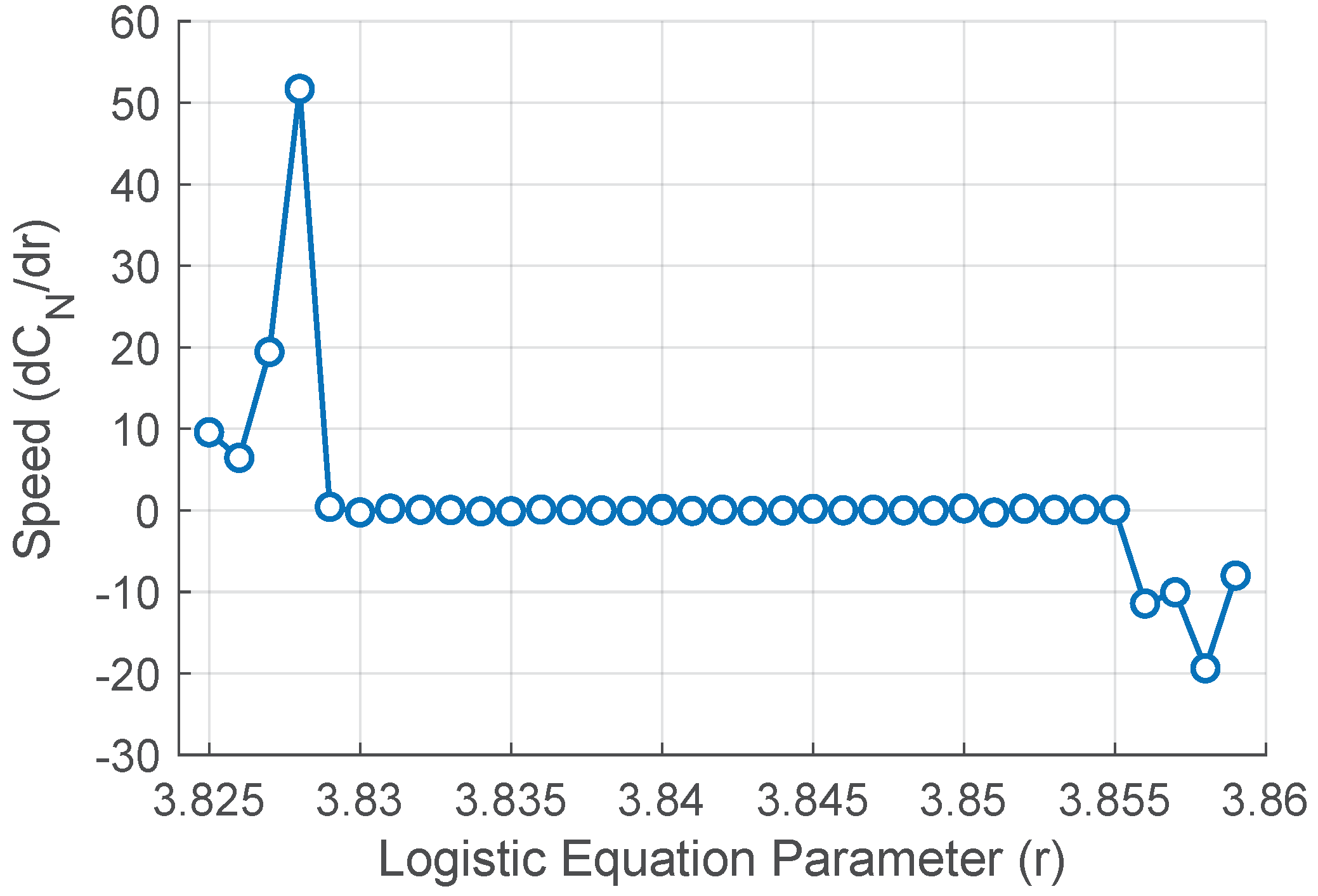
It can be seen that the entry and exit of the stable zone is "smooth", as a anticipation of the behavior change. This becomes very clear when the speed () is calculated at which it approaches stability and the speed at which it moves away ((Figure 8).
Figure 8.
Speed () when entering and leaving the stable island shown in Figure 7. Note the sharp peaks at the transitions.
Figure 8.
Speed () when entering and leaving the stable island shown in Figure 7. Note the sharp peaks at the transitions.
5. Discrete Virial Formalism and Chaotic Maps
5.1. Convergence Velocity as Chaos Indicator
This section analyzes the convergence velocity of the discrete Virial coefficient () for three well-known iterated maps capable of exhibiting chaotic behavior. Specifically, were selected the logistic map (a second-degree polynomial), the discubic map (a third-degree polynomial), and the sin map (utilizing the periodic trigonometric iterated function). This investigation is partly motivated by the work of Howard [12], which addresses the convergence of a discrete Virial theorem in Hamiltonian systems. The logistic map was introduced in the previous section in the Equation (14), the choice for the parameter r∈ was fixed in 4 for the chaotic regime, and 3.4 for the non-chaotic.
The discubic discrete map [18] is defined by:
where the parameter a∈ was settled equal to 3.8 for the chaotic regime, and equal to 1.28 for the non-chaotic one.
The other iterative map analyzed was the sin map [19], which can be expressed as:
where w∈ was selected to 3.8 for chaotic behavior and 1.28 for non-chaotic.
To estimate the convergence velocity of the coefficient (, defined in Equation (13)) for both chaotic and non-chaotic regimes, a convergence velocity coefficient () was implemented. The is computed by segmenting the time series into K windows, each of size M. For each window j the mean discrete Virial coefficient () is calculated, and is then determined using:
In Equation (17), is the discrete Virial coefficient at point i within a given window, is the mean Virial coefficient for the window (i.e., , and j indexes these windows from 1 to K). Equation 17 was used to compute the values from the series of the iterated maps, considering parameter values that yield both chaotic and non-chaotic regimes. Then, a comparative metric was defined to contrast these behaviors for each map:
where is the standard deviation.
The results of the experiments using the expression 18 are shown in Table 1, in which the window size applied was 100 data points.
Howard [12] (in Section 5 of that work) proposed a chaos indicator based on the convergence rate of the average kinetic energy. Based on this, the present study shifts focus to analyzing the convergence properties of the discrete Virial coefficient () itself, which contains information from both kinetic () and potential () factors. The aim is to extend these concepts to a wider range of time series and numerically determine the convergence rate of .
However, the direct convergence of can be oscillatory for non-chaotic trajectories and highly irregular (rough) for chaotic ones. To mitigate these fluctuations and obtain a more stable measure of convergence, the standard deviation of was analyzed instead of a direct computation on the coefficient .
5.2. Discrete Virial Coefficient and Order Windows
It is well established that the change of behavior of a dynamical system between the chaotic and non-chaotic regime can be tracked in various ways, for example by the phase diagram, or by the bifurcation diagram, or by calculating the Lyapunov exponents. In this subsection is presented a novel result in which the discrete Virial coefficient plays a fundamental role and also provides an interpretation based on concepts related to the potential and kinetic factors of the discrete Virial ratio. Figure 9a) shows the Feigenbaum bifurcation diagram for the logistic equation, below is the calculation of the discrete Virial coefficient for the same expression Figure 9b), and below it is the calculation of the Lyapunov exponent for the same map as shown in Figure 9c). The figure above clearly shows the ordering windows once the logistic equation develops the chaotic regime, in the figure below it is observed that for each of these windows the shows an interval of approximately constant value. This fact can be confirmed by looking at the figure showing, the Lyapunov exponent, which is an established indicator for this type of behavior. The former case of the logistic equation is mathematically represented by a polynomial of second degree, in the Figure 10 analogous results are shown for the discubic equation presented before but in this case for a recursive polynomial of third degree. The results obtained for the sin map are shown in the Figure 11, meanwhile, the final case is exhibited in the Figure 12, in which case the Gaussian map [19] was studied whose expression is given by:
where the ∈ was fixed in 8 and the parameter ∈ ranging from -1 to 1.
Figure 9.
Logistic map: a) Feigenbaum Bifurcation Diagram, b) Virial Coefficient plot, c) Lyapunov Exponent.
Figure 9.
Logistic map: a) Feigenbaum Bifurcation Diagram, b) Virial Coefficient plot, c) Lyapunov Exponent.
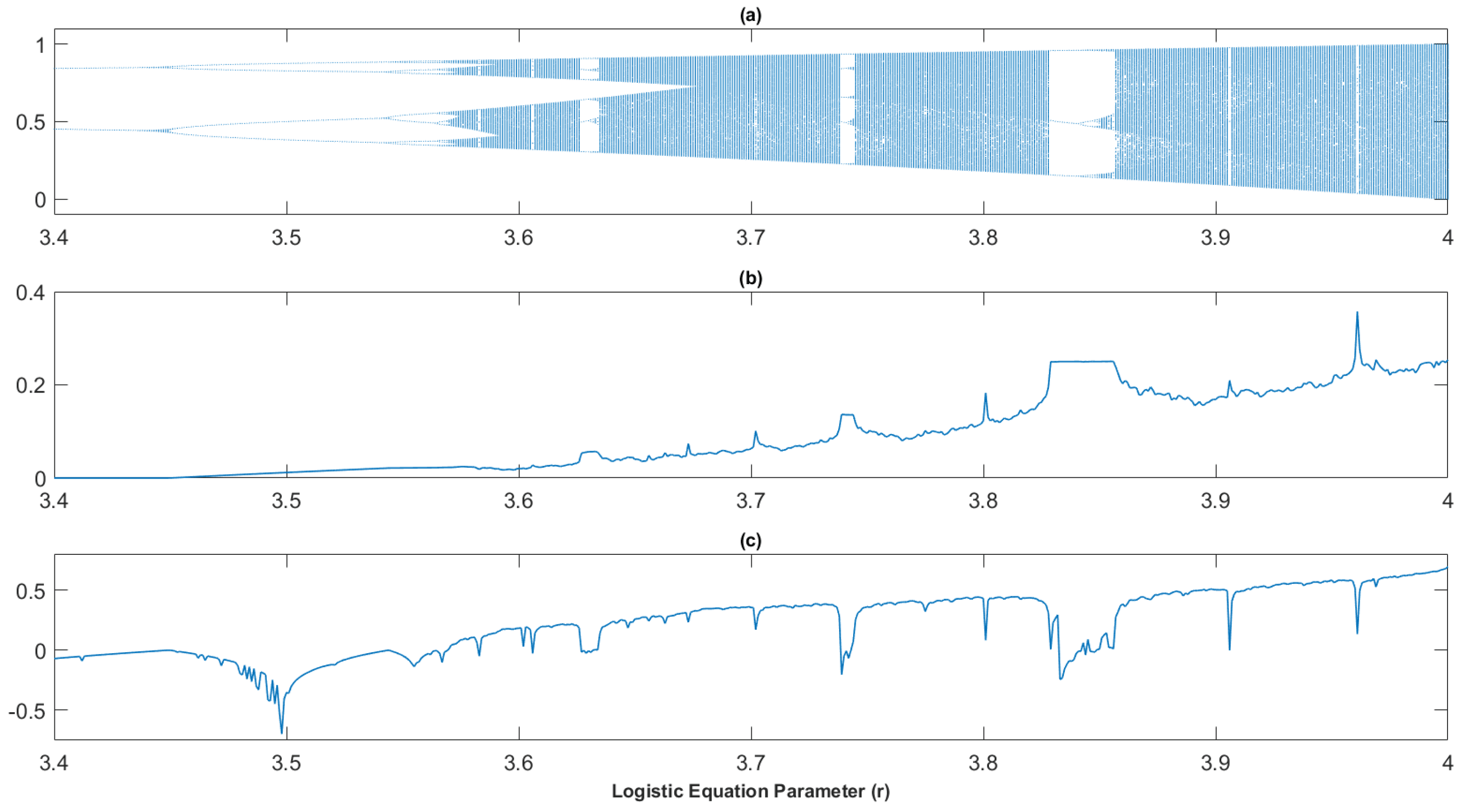
Figure 10.
Discubic map: a) Feigenbaum Bifurcation Diagram, b) Virial Coefficient plot, c) Lyapunov Exponent.
Figure 10.
Discubic map: a) Feigenbaum Bifurcation Diagram, b) Virial Coefficient plot, c) Lyapunov Exponent.
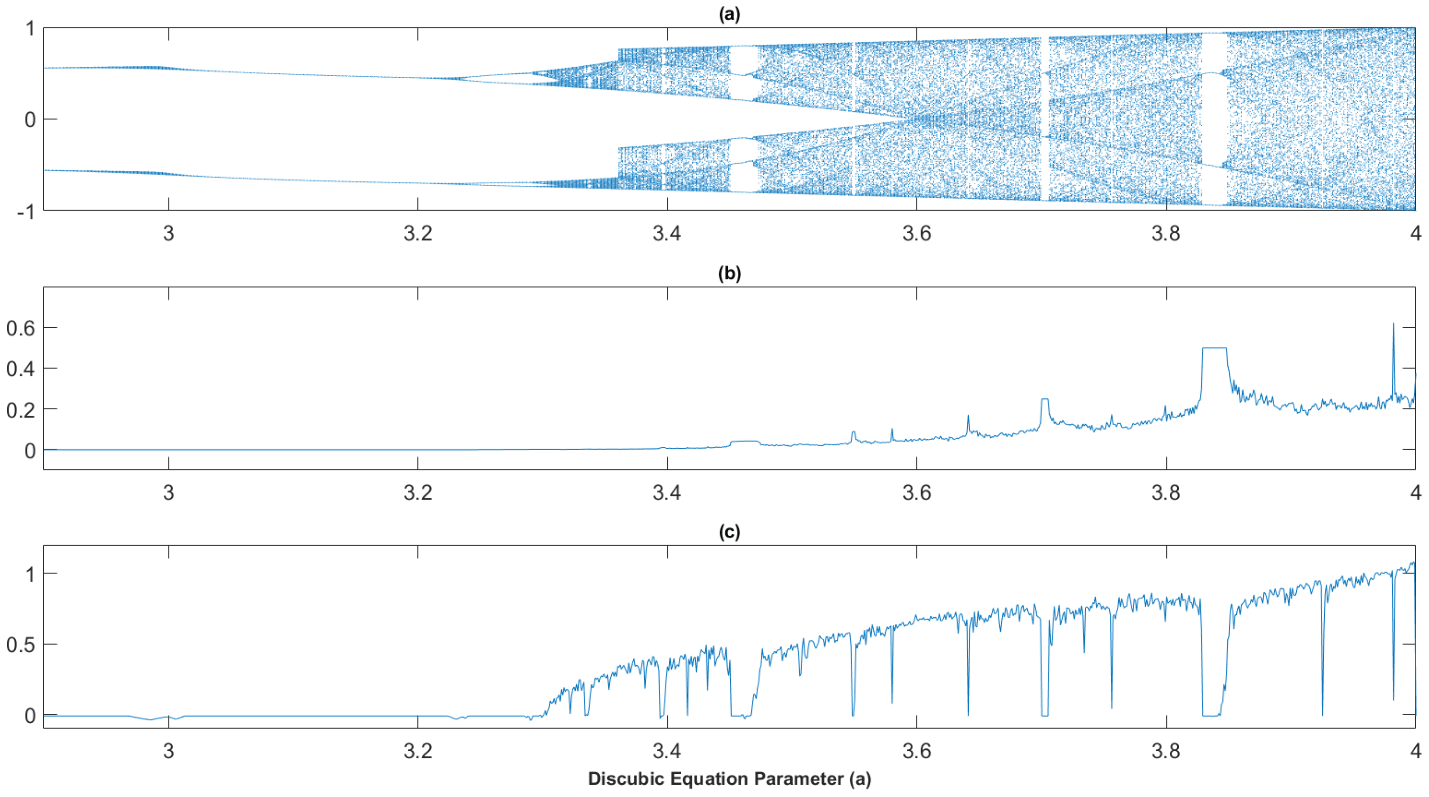
Figure 11.
Sin map: a) Feigenbaum Bifurcation Diagram, b) Virial Coefficient plot, c) Lyapunov Exponent.
Figure 11.
Sin map: a) Feigenbaum Bifurcation Diagram, b) Virial Coefficient plot, c) Lyapunov Exponent.
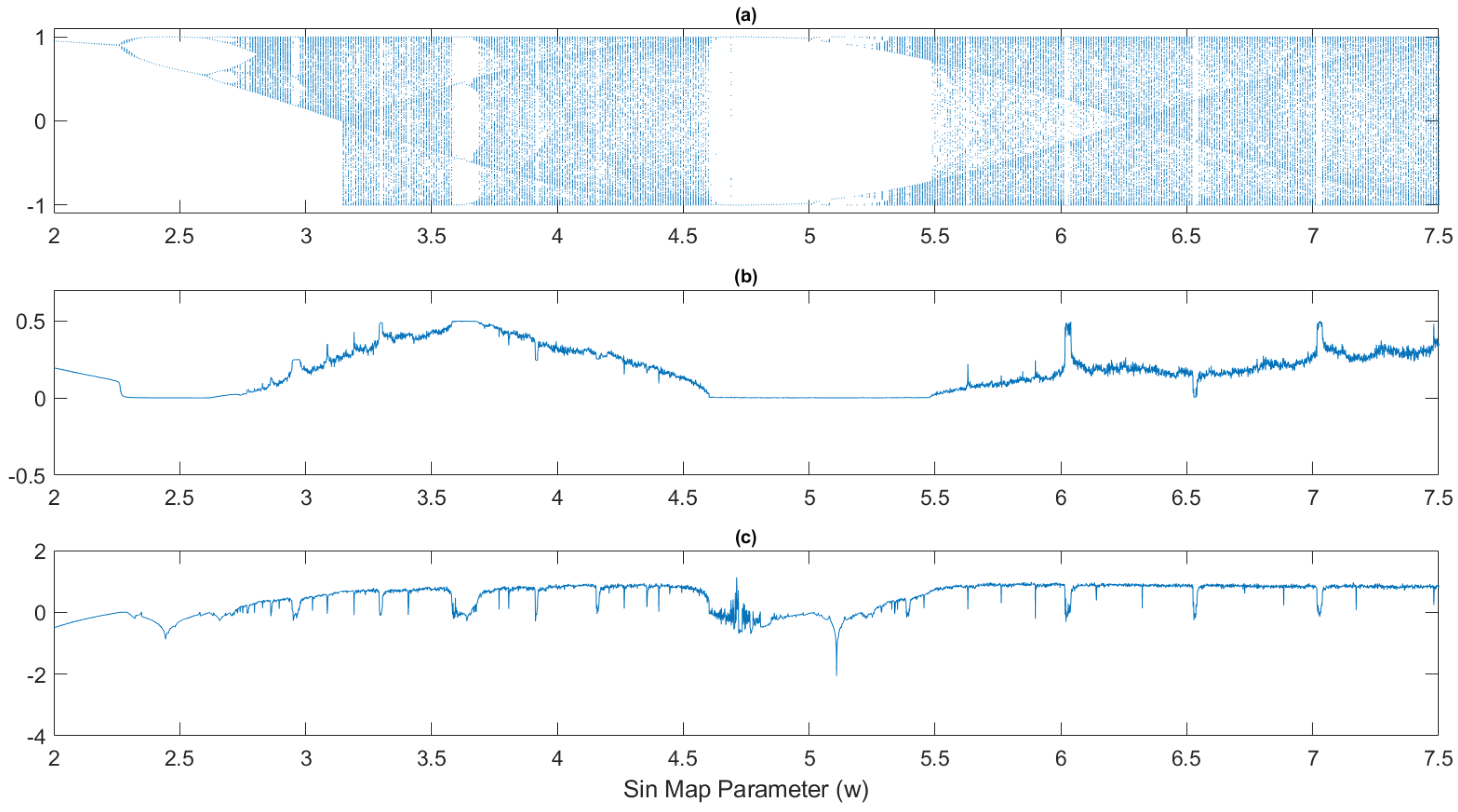
Figure 12.
Gaussian map: a) Feigenbaum Bifurcation Diagram, b) Virial Coefficient plot, c) Lyapunov Exponent.
Figure 12.
Gaussian map: a) Feigenbaum Bifurcation Diagram, b) Virial Coefficient plot, c) Lyapunov Exponent.
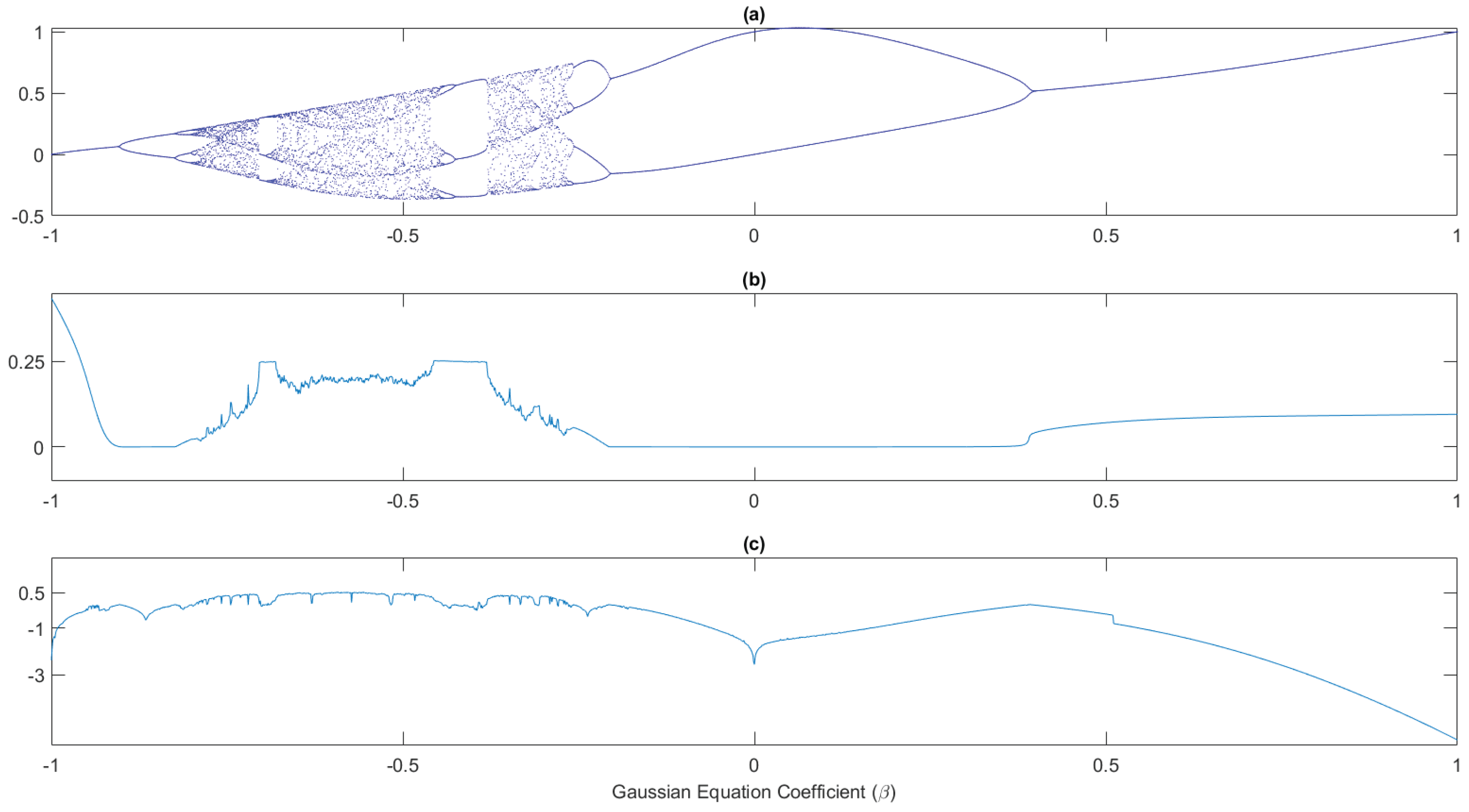
From Figure 9 to Figure 12 is clear to note that when each time the dynamical the system described by the corresponding equation enters in a ‘window’ of order, as can be seen in the previous mentioned figures, in all cases, the discrete Virial coefficient shows a plateauing that accompanies such transitions. This fact can be interpreted with the help of the discrete extension of the Virial theorem proposed in this work, in such a way as to think that the transient ordering in the exhibited iterated maps corresponds to a compensation of the terms associated with the kinetic and potential components of coefficient given by the expression 13. This is a new result not found in the available literature and could indicate that the discrete Virial coefficient could be used as a proxy or indicator of the ordering windows in discrete chaotic iterated maps.
The time involved in calculating the Virial coefficient is at least one order of magnitude less than the time required to calculate the Lyapunov exponent; in this research the Lyapunov exponent was calculated using the algorithm in [20]. Performance was computed with a code in the Octave language version 10.2.0 and running on a Core i7 processor with 32 Gb of RAM.
6. Discrete Virial Formalism Applied to Experimental Series
The proposed extension of the discrete Virial coefficient was tested using data acquired with continuous-glucose-monitor (CGM) from five healthy and five diabetic volunteers. For datils see [21]; the sampling time was = 5 min, and series length was composed by 10,000 data points. In such a way, two sets of five data series, containing healthy and diabetic subject records, were obtained according to the procedure described in the reference. In parallel, these data were interpolated with the cubic spline, resulting in two additional series. The discrete Virial coefficient was computed on each data record and calculated the mean and its dispersion of the value of on the last 400 values of the series of 10,000 data points, see Table 2.

Table 2.
Mean and Variance of Virial coefficient (N=5 individuals).
| H. raw | H. int | S. raw | S. int | |||||
|---|---|---|---|---|---|---|---|---|
| ID | M | V | M | V | M | V | M | V |
| 1 | 0.7315 | 0.0138 | 1.0410 | 0.0131 | 0.8764 | 0.0094 | 1.0772 | 0.0055 |
| 2 | 0.6617 | 0.0103 | 0.9849 | 0.0054 | 0.7861 | 0.0137 | 0.9973 | 0.0149 |
| 3 | 0.6519 | 0.0121 | 0.9845 | 0.0111 | 0.7777 | 0.0155 | 0.9948 | 0.0091 |
| 4 | 0.6570 | 0.0078 | 1.0057 | 0.0083 | 0.8329 | 0.0198 | 1.0067 | 0.0262 |
| 5 | 0.7134 | 0.0096 | 1.0042 | 0.0058 | 0.8929 | 0.0146 | 1.0092 | 0.0107 |
H. raw: Healthy without interpolating; H. int: Interpolated healthy; S. raw: Sick without interpolating; S. int: Interpolated sick; M: Mean ; V: Variance. Calculated on last 400 points of N=10000 series.
The scatter of the last 400 data ensures that the variance over the 5 values of each group in Table II corresponds to variations between individuals rather than to variations in the Virial coefficient . The result of this is shown in Table 3 and in Figure 13.
Table 3.
Average Virial coefficient and Inter-individual Variance for Glucose Data Groups (summarized from reference).
Table 3.
Average Virial coefficient and Inter-individual Variance for Glucose Data Groups (summarized from reference).
| Group | Average | Variance (between individuals) |
|---|---|---|
| Non-diabetics, raw data | 0.6831 | 0.0327 |
| Non-diabetic interpolated data | 1.0040 | 0.0205 |
| Diabetics, raw data | 0.8332 | 0.0463 |
| Diabetic interpolated data | 1.0170 | 0.0305 |
Summarized from previous detailed individual data.
Figure 13.
Discrete Virial coefficient ()evaluated for biological series (glucose data) with and without data interpolation (Graphical representation of Table 3), the circles represents the mean values of and the vertical segments corresponds to the variation within earch group
Figure 13.
Discrete Virial coefficient ()evaluated for biological series (glucose data) with and without data interpolation (Graphical representation of Table 3), the circles represents the mean values of and the vertical segments corresponds to the variation within earch group
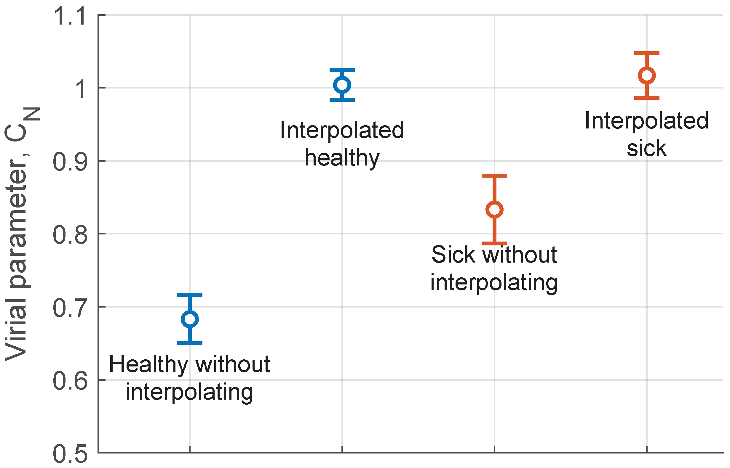
Two important results emerge from Figure 13 which is a conceptual scheme: a) For the data without interpolation, the parameter clearly distinguishes diabetics from non-diabetics; b) When the data are interpolated, this difference disappears and the value of the parameter approaches unity, a characteristic of the data generated by a differential equation [21]. Using a previously published formalism [21], it is also verified that interpolation erases the difference between diabetics and non-diabetics. The Virial Transformation shows that an interpolation process to smooth experimental data from a series can distort the information originally contained in the series.
7. Results Analysis
In This research was introduced an extension of the Virial formalism to discrete systems like as numerical solution of nonlinear differential equation, some discrete systems, discrete chaotic iterative maps, and measured data, some interesting properties had emerged from the cases analyzed that are affordable to continue investigating.
The analysis of the series generated by the double pendulum solution in Section 4.1.1 shows that convergence of the discrete Virial coefficient is very good and sufficiently fast for nonlinear Hamiltonian systems.
As shown in Figure 5, the convergence demonstrates that the factors and evolve in a nearly identical manner, resulting in an approximate convergence of the parameter . Specifically, after approximately 500 iterations, the relationship between the factors identified as kinetic and potential factors remains constant, favoring the associated with the potential energy in a 75%. This result holds when taking the inverse of the pseudorandom numbers; furthermore, the need for the series to be bounded becomes evident.
The Figure 6 shows how the value of varies with the initial conditions before the bifurcation of the logistic equation in the vicinity of the parameter , highlighting how the slopes of the decrease in the discrete Virial coefficient change at the entrance and exit of the mentioned bifurcation. This fact could be used to predict the entry of the logistic equation dynamics into a bifurcation. On the other hand, Figure 7 shows the plateau formed by when the logistic equation enters a zone of stability after having developed chaotic behavior at its extremes. Furthermore, Figure 8 shows the difference in the speed with which the evolution of the logistic equation enters the zone of stability and with which it exits that zone.
In Appendix A there is a brief discussion about the effect of the time-step size in the results of the convergence of the discrete Virial coefficient. And in Appendix B is showed how the noise can disturb the Virial value of a perfect differentiable function.
As can be seen in Table 1, for the three iterated maps considered, the standard deviation of the numerator of the Equation (18) is smaller than the standard deviation calculated for the denominator. This is indicating that the Virial discrete coefficient reaches its final value faster when the iterated map is applied with its parameter set to exhibit non-chaotic behavior than when it is applied under the chaos conditions. Depending on the components of the discrete Virial Equation (13), one associated with the kinetic component and the other with the potential, the slower speed of convergence could be interpreted as a greater imbalance between these two components when the system is starting up under chaotic conditions. This would be exactly the opposite in the case of the behavior of the same system running under non-chaotic conditions.
The Figure 9 a) shows several ordering windows of the Feigenbaum diagram for the logistic map. The most extended ones are centered on the values of the parameter r approximately 3.65, 3.75 and 3.85, in all three cases the verification of the class of behavior can be confirmed with the calculation of the corresponding Lyapunov exponent as can be seen in Figure 9c), note that in Figure 9b) appear plateaus of almost constant behavior of the discrete Virial coefficient. This fact shows that both components that has been agreed to be defined as kinetic and the potential factors are found in areas where the quotient provided by the coefficiente is almost constant. This could be a new framework that employs the constancy of the discrete Virial coefficient as a proxy of the ordering windows of bifurcation diagram of the logistic iterated map.
For the case of the discubic map in Figure 10a), a similar behavior of the discrete Virial coefficient was found when an ordering window occurs in the bifurcation diagram. This case being an iterated map of degree three to analyze whether the behavior found for the logistic map was reiterated in this new case.
To analyze other case more of the presence of the plateaus as a proxies of the ordering windows, an iterated map defined on a periodic function was selected, as the case of the sin map. In the Figure 11a), shows a narrow window centered at approximately , a wide window between 4.6 and 5.3 and much narrower windows around 6, 6.5 and 7. This phenomenon is reflected with the Lyapunov exponent in Figure 11c), and the presence of plateaus in the coefficient can be observed in the regions corresponding to the same parameter values in the Figure 11b), which is another confirmation of the phenomenon found with the behavior of the discrete Virial coefficient in the regions of the order in the bifurcation diagrams.
The last case analyzed in the Subsection 5.2 is the order windows in the Gaussian map. This map was selected because is composed by a exponential function and have a wide range of order in the bifurcation diagram as can be seen in the Figure 12a). This map, whose bifurcation diagram is shown in Figure 12a) has a window of order whose center is close to the value of the parameter -0.7, another one a bit wider centered around -0.3 and a very large one starting from the parameter close to -0.2. In all the cases it is possible to appreciate the presence of a plateau in the value of the discrete Virial coefficient, as it is observed in Figure 12b), and additionally as in all the previous analyses it is attached in Figure 12c) the corresponding calculation of the Lyapunov exponent. In all exposed cases, there are much narrower windows of order that are not analyzed in detail but which a deep revision of the graphs makes evident.
Two important results emerge from Figure 13: a) For the data without interpolation, the parameter clearly distinguishes diabetics from non-diabetics; b) When the data are interpolated, this difference disappears and the value of the parameter approaches unity, a characteristic of the data generated by a differential equation; see Figure 1. Previous treatments have also shown this result; interpolation erases the difference between the signals. The discrete Virial extension shows that an interpolation process to smooth experimental data from a series can distort the information originally contained in the series.
8. Conclusion
This work has demonstrated the feasibility of applying the Virial concept to discrete systems, even in cases that do not have a Hamiltonian and in some cases with problems in defining the concept of discrete derivative. However, the quotient established in the discrete definition of Virial can continue to be applied to obtain the relevant properties of the data series analyzed. The convergence towards a given value of was also verified in the numerical solution of the non-linear differential equation of the double pendulum. In addition, it was verified in some systems such as pseudorandom number generators and in the equation of the logistic iterative map.
The speed with which the coefficient of the discrete Virial tends to its final value after a number of applications of the iterated maps has been shown to be a discriminator of the behavior of the maps. In the chaotic regimes, it has shown with reference to the non-chaotic ones a slower convergence speed, as shown by the coefficient designed ad hoc in the present research. Given a number of samples from a dynamic system, and without information on its operating regime, a comparison of the speed of convergence of the discrete Virial coefficient could be made to find out the behaviour of the systems. This fact represents in itself another contribution in quasi-energetic terms, given that the greater convergence of the Virial coefficient implies a smaller oscillation of it in the initial moments of the operation of a dynamic system, which translates into a smaller oscillation of the quotient between the term associated with the kinetic component and that of the potential component, which precisely constitutes the coefficient of the discrete Virial.
One of the main contributions of this work can be represented by the association of the intervals of values of the discrete Virial coefficient almost constant, as a proxy of the emerging of the ordering windows in the Feigenbaum diagrams of the logistic, discubic, Sin map and Gaussian maps. In all of them, every time a simplification of the bifurcation diagram begins to appear, an approximated compensation of the kinetic and potential therms of the expression for the discrete Virial Coefficient is present. This ordering windows in chaotic maps is a well-known fact that could be reinterpreted in terms of the discrete Virial coefficient from a nearly energetic point of view. More explicitly, because it can be associated with an equilibrium in the relationship between the kinetic energy and potential energy components of the discrete Virial extension.
Finally it was applied to a series of measured blood glucose density data that demonstrated the capacity of the discrete extension of the proposal to study the differentiation of time series.
As a final summary, it can be concluded that the extension of the discrete Virial formalism presented here has a clear conceptual simplicity and ease of computational implementation which, in relation to the properties it could provide of the data series to be analyzed, presents as a very interesting and innovative alternative which only requires that the discrete data series should to be bounded.
Author Contributions
All the authors contribute in the same way to the production of this research.
Acknowledgments
The authors wish to acknowledge the support of the Universidad Tecnologica Nacional Projects: Signal Analysis Using Geometric Transformations and Symbolic Sequences and Informational Tools, Project Code PID ASIFNBA0010125, and Study of the Glucemic Dynamic of Subjects Suffering Type II Diabetes Through Mathematical Models and Informational Theory, Project Code PID de PID ASPPGP0010154.
Conflicts of Interest
The authors declare no conflicts of interest.
Appendix A. On the Role of the Sampling Interval (h)
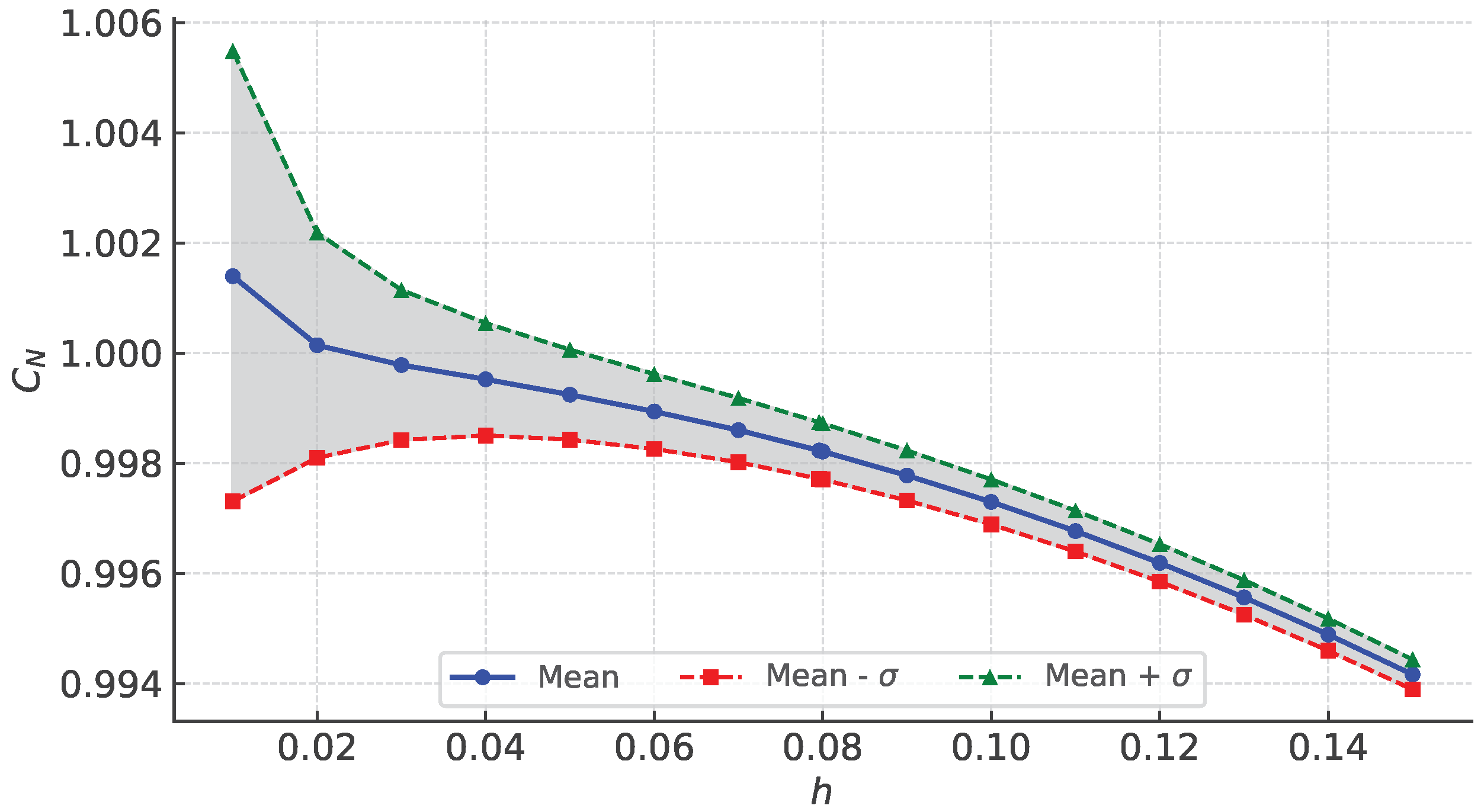
This appendix is devoted to the analysis of what happens if the calculation step h is still constant, but with a different value. Although does not depend on h theoretically, the signal can be distorted by the size of the interval between signal data, and therefore the information conveyed by the series varies. This is a complicated problem, and there are three possible situations: a) it is possible to vary h arbitrarily, b) it is possible to vary h to some extent, and c) it is not possible to vary h.
Case a) occurs for solutions of differential equations, and adjusting the value of h to small values gives the value of . In c) the case in which the solutions of difference equations, like pseudorandom numbers and logistic map, where by construction and it cannot be varied. Finally, case b) is actually the most important because it will be presented in the study of experimentally obtained series. In this case, when physical and/or biological quantities are measured numerically, the signal is inherently discrete and the value of h is usually given by the experiment itself or by the measuring device. Normally, experiment and measurement equipment are designed with the objective of obtaining a series for which h is as small as possible. In any case, the series information corresponds to the set of experimental/measuring device.
For the case of the function , see Figure A1 that illustrates the problem that arises when the sample size h is varied.
Figure A1.
Variation of average (blue line) and its standard deviation band (sigma) when varying the sampling interval h for , where refers to the standard deviation.
Figure A1.
Variation of average (blue line) and its standard deviation band (sigma) when varying the sampling interval h for , where refers to the standard deviation.
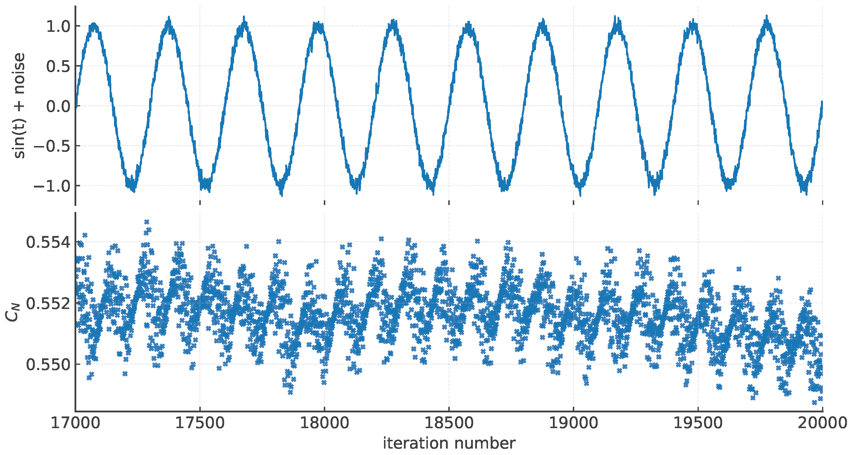
Appendix B. Impact of Discontinuities in Analyzed Series
Returning to the case of the solution of a harmonic oscillator with the function , this time disturbed by pseudorandom noise. The point here is to determine how the signal begins to lose the information of the derivatives. By adding pseudorandom "noise" in different proportions, Table A1 examines the sensitivity of . It can be seen that decreases and quickly approaches the value of obtained with pseudorandom numbers (approx. 0.25).
Table A1.
Evolution of the mean of (between iterations 15000 and 20000) and the corresponding variance when adding pseudorandom (0-1) noise to . Calculation used time sptep .
Table A1.
Evolution of the mean of (between iterations 15000 and 20000) and the corresponding variance when adding pseudorandom (0-1) noise to . Calculation used time sptep .
| Noise Added | Variance | |
|---|---|---|
| 0% | 1.0000 | 0.0017 |
| 1% | 0.9623 | 0.0017 |
| 5% | 0.5675 | 0.0017 |
| 10% | 0.3645 | 0.0004 |
| 20% | 0.2823 | 0.0006 |
| 50% | 0.2596 | 0.0005 |
| 100% | 0.2497 | 0.0006 |
In Figure A2, it can be seen that a small disturbance is generated by adding 5% noise [14] to the signal produces a large variation in the evolution of the value. The convergence of to the value generated by the pseudorandom numbers occurs for any proportion when the pseudorandom numbers are multiplied rather than added.
Figure A2.
Evolution of adding 5% of pseudorandom (0-1) noise and the corresponding evolution of after 17000 iterations.
Figure A2.
Evolution of adding 5% of pseudorandom (0-1) noise and the corresponding evolution of after 17000 iterations.
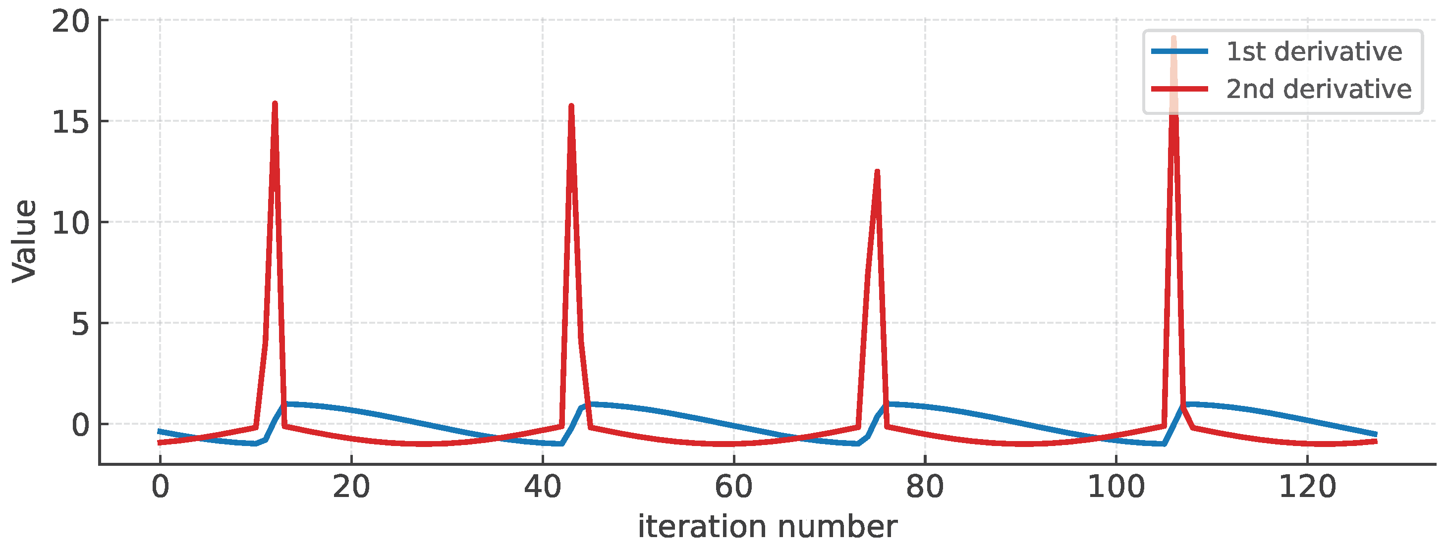
Having clarified this point, the problem that arises is to find out which analytic functions are close to and which are outside the dispersion of this value. For example, approaches . Instead, this function:
Converges to: . This function is continuous, but not its derivative, looking closely the first derivative changes sign at the cusps.
This function has the first derivative similar a Heaviside discontinuity, going from negative to positive. Consequently, the second derivative has a "delta" type discontinuity: between two negative values, it grows to a positive value (see Figure A3). It is concluded that the values that can take are strongly influenced by the degree of continuity of the derivatives of the data series.
Figure A3.
Derivatives of the function .
References
- Goldstein, H. Classical Mechanics, 2nd ed.; Addison-Wesley, 1980.
- Alazard, T.; Zuily, C. Virial theorems and equipartition of energy for water waves. SIAM Journal on Mathematical Analysis 2024, 56, 5285–5329. [Google Scholar] [CrossRef]
- López-Corredoira, M.; Betancort-Rijo, J.; Scarpa, R.; Chrobáková, Ž. Virial theorem in clusters of galaxies with MOND. Monthly Notices of the Royal Astronomical Society 2022, 517, 5734–5743. [Google Scholar] [CrossRef]
- Shneerson, G.; Shishigin, S. Features of the application of the virial theorem for magnetic systems with quasi-force-free windings. Technical Physics 2023, 68, S595–S606. [Google Scholar] [CrossRef]
- Pommaret, J. From Thermodynamics to Gauge Theory: The Virial Theorem Revisited. Gauge Theories and Differential Geometry, NOVA Science Publisher, Hauppauge, 2015; 1–46. [Google Scholar]
- Marc, G.; MacMillan, W.G. The virial theorem. Advances in Chemical Physics 2007, 58, 209–361. [Google Scholar]
- Jones, R.O. Density functional theory: Its origins, rise to prominence, and future. Reviews of modern physics 2015, 87, 897–923. [Google Scholar] [CrossRef]
- Cariñena, J.F.; Falceto, F.; Ranada, M.F. A geometric approach to a generalized virial theorem. Journal of Physics A: Mathematical and Theoretical 2012, 45, 395210. [Google Scholar] [CrossRef]
- Cariñena, J.F.; Muñoz-Lecanda, M.C. Revisiting the generalized virial theorem and its applications from the perspective of contact and cosymplectic geometry. International Journal of Geometric Methods in Modern Physics 2025, 22, 2450269. [Google Scholar] [CrossRef]
- Mathews, J.H.; Fink, K.D. Métodos Numéricos; Prentice Hall: Madrid, 2000. [Google Scholar]
- Kocak, H. Differential and difference equations through computer experiments; Springer Science & Business Media, 2012.
- Howard, J.E. Discrete Virial Theorem. Celestial Mechanics and Dynamical Astronomy 2005, 92, 219–241. [Google Scholar] [CrossRef]
- Calvão, A.; Penna, T. The double pendulum: a numerical study. European Journal of Physics 2015, 36, 045018. [Google Scholar] [CrossRef]
- Matsumoto, M.; Nishimura, T. Mersenne Twister: A 623-Dimensionally Equidistributed Uniform Pseudo-Random Number Generator. ACM Transactions on Modeling and Computer Simulation 1998, 8, 3–30. [Google Scholar] [CrossRef]
- Feigenbaum, M.J. Quantitative universality for a class of nonlinear transformations. Journal of Statistical Physics 1978, 19, 25–52. [Google Scholar] [CrossRef]
- Landford, III, O.E. A computer-assisted proof of the Feigenbaum conjectures. In Universality in Chaos; Cvitanović, P., Ed.; Routledge, 2017; pp. 245–252.
- Pomeau, Y.; Manneville, P. Intermittent transition to turbulence in dissipative dynamical systems. Communications in Mathematical Physics 1980, 74, 189–197. [Google Scholar] [CrossRef]
- May, R.M. Bifurcation and dynamic complexity in ecological system. Annals of the New York Academy of Sciences 1979, 316, 517–529. [Google Scholar] [CrossRef]
- Lynch, S. Dynamical systems with applications using python; Springer, 2018.
- McCue, L.S.; Troesch, A.W. Use of Lyapunov exponents to predict chaotic vessel motions. In Contemporary ideas on ship stability and capsizing in waves; Springer, 2011; pp. 415–432.
- Amadio, A.; Rey, A.; Legnani, W.; Blesa, M.G.; Bonini, C.; Otero, D. Mathematical and informational tools for classifying blood glucose signals - a pilot study. Physica A: Statistical Mechanics and its Applications 2023, 626, 129071. [Google Scholar] [CrossRef]
Table 1.
Comparison of Virial Velocity convergence for iterated maps according to chaotic and non-chaotic behavior
Table 1.
Comparison of Virial Velocity convergence for iterated maps according to chaotic and non-chaotic behavior
| CC/Iteration | 500 | 1000 | 5000 | 10000 | 50000 | 100000 | 150000 | 200000 |
|---|---|---|---|---|---|---|---|---|
| Logistic | 7.3927 | 0.5682 | 0.2924 | 0.0736 | 0.0565 | 0.0083 | 0.0083 | 0.0083 |
| Discubic | 0.1184 | 0.0932 | 0.0274 | 0.0272 | 0.0257 | 0.0257 | 0.0257 | 0.0257 |
| Iterated Sin | 0.0076 | 0.0076 | 0.0075 | 0.0056 | 0.0055 | 0.0040 | 0.0033 | 0.0013 |
Comparison using Equation (17).
Disclaimer/Publisher’s Note: The statements, opinions and data contained in all publications are solely those of the individual author(s) and contributor(s) and not of MDPI and/or the editor(s). MDPI and/or the editor(s) disclaim responsibility for any injury to people or property resulting from any ideas, methods, instructions or products referred to in the content. |
© 2025 by the authors. Licensee MDPI, Basel, Switzerland. This article is an open access article distributed under the terms and conditions of the Creative Commons Attribution (CC BY) license (http://creativecommons.org/licenses/by/4.0/).
Copyright: This open access article is published under a Creative Commons CC BY 4.0 license, which permit the free download, distribution, and reuse, provided that the author and preprint are cited in any reuse.


