
Submitted:
22 September 2025
Posted:
23 September 2025
You are already at the latest version
Abstract
The sun-tracker plays a major role in improving the energy efficiency of the solar system. To address this gap, this study experimentally explores the energy efficiency of three sun-tracking systems with three types of degrees of freedom (DOF), namely: single-axis for both elevation (1DOF_Elev) and azimuth (1DOF_Azim), and dual-axis (2DOF), integrated in photovoltaic (PV) panels. The three sun-tracking configurations are assessed and compared with the fixed system (0DOF), considering both the net electricity output of the studied photovoltaic system and the energy consumption of each configuration during operation. To accomplish this objective, hardware and software tools were deployed to create a prototype. The sun-tracking techniques are based on the sun position algorithm (astronomical calculations). The different data (time, voltage, current, power, azimuth and elevation) are stored in real time within a locally developed database which represents crucial data within SCADA systems embedded in smart grids. The results revealed that the 2DOF system exhibits the highest energy efficiency (37.23%) followed by 1DOF_Azim (12.86%) and then by 1DOF_Elev (10.05%), when compared to 0DOF. Overall, this study provides solutions for optimizing photovoltaic energy production and could be integrated into battery-powered devices, to accelerate battery recharging, achieving time savings of over 30%.
Keywords:
battery
; data digitization
; energy efficiency
; photovoltaic
; optimizing energy
; smart-grid
; sun-tracking
1. Introduction
Sun trackers are key devices in adjusting the position of the solar collectors towards the sun to maximize the solar energy collected and hence improving their efficiency [1]. In the literature, many previous works confirmed this role. Certainly, according to Mousazadeh et al. [2], sun trackers can improve the absorbed energy by 10 to 100% across different geographical locations and seasons. Eke et al. [3] noted that a sun tracking system, compared to a latitude tilt fixed system, could increase the annual photovoltaic electricity output of a 7.9 kW photovoltaic (PV) system installed at Mugla University by 30.79%. Similarly, experimental studies by Khalifa et al. [4] and Abdallah et al. [5] on different solar collectors revealed that the solar energy collected was higher than that of fixed collectors, with increases of 75% and 41.34%, respectively. Thanks to these incontestable performances, sun tracking systems are widely incorporated into commercial scale solar installations around the globe. This diversity in design has led to extensive research and analysis by numerous experts, since their first outbreak in 1927 [6]. From a state-of-the-art perspective, sun tracking systems have been grouped based on various parameters such as control and tracking strategies, drives, and degrees of freedom [7,8].
In the literature, these systems are classified into three technological classes: thermo-hydraulic actuator mechanism [9], bimetallic thermal actuator mechanism [10] and shape memory alloy thermal actuator mechanism [11]. However, they can mainly be divided into two types: passive and active trackers. Passive trackers are typically used for PV systems as they do not require any electrical energy or mechanical drives. They operate based on autonomous physics phenomena to create motion. Conversely with passive trackers, the active ones use sensors, predefined algorithms, and electrical motors to predict or calculate the sun’s current position and adjust the reflector’s alignment so that the collector’s normal vector is perpendicular to the sun’s rays [12]. Depending on their tracking strategy, active trackers can be categorized into two types [13]: astronomical trackers and electro-optical sensor-based trackers. The astronomical trackers operate solely on calculations of the apparent sun’s position, using predefined geometric and astronomical equations. This method, also known as an open loop or blind technique, relies exclusively on ephemeris calculations without direct measurements of the sun’s position. It requires manual adjustments to set the latitude, date, and time on the first day of operation. Subsequent automatic computations and commands are handled by a preprogrammed processor, regardless of external conditions such as wind speed or climate changes. For example, Canada et al. [14] developed an automatic device to measure global irradiance, total atmospheric optical thickness, aerosol optical depth, and direct irradiance. This tracker was developed using C++ builder and based on the mathematical correlations proposed by Blanco-Muriel et al. [15]. Similarly, Alata et al. [16] introduced a new open loop sun tracking system using a fuzzy model to represent the mathematical equations for determining the sun’s position in Amman, Jordan. They designed three tracking systems: one-axis tracking, equatorial tracking, and azimuth/elevation tracking.
On the other hand, the electro-optical sensor-based trackers, unlike the open loop technique-based trackers, rely on tangible feedback from electro-optical sensors such as light sensors, photo-resistors, and PV cells. This method, known as the closed loop technique, operates by adjusting the solar collector’s position to ensure that the illumination on the light sensors is balanced. To assess the pertinence of this sensor tracking approach, Boukdir et al. [17] have developed a new dual-axis solar tracker that uses three Light Dependent Resistors (LDRs) as optical sensors: one on the left, one on the right for azimuthal tracking, and a central one for elevation tracking.
Far from the technical classification of solar tracking systems based on the technique deployed to control the mechanical movement, several other painstaking publications assessed the economic and the energy impact of different tracking approaches based on the system’s degree of freedom. Indeed, based on this criterion, the sun trackers can be classified in two categories: single-axis and dual-axis trackers. The working principle of the former is to rotate the solar collector around a single horizontal, vertical, polar, or inclined axis to reduce as much as possible the incidence angle [18]. However, this technique is difficult to apply in large-scale plants because of high costs and land requirements [19].
Several researchers have explored, through simulations or experiments, ways to find a balance between different tracking modes. Their goal is to maximize the benefits of each approach while minimizing their drawbacks. For instance, through a series of numerical simulations comparing five tracking configurations, Maia et al. [1] have confirmed that the dual-axis sun tracking mode remains the best option to enhance the installation’s thermal efficiency. Ai et al. [20] have proposed and compared two sun tracking methods to optimize a PV system’s performance in Er-Lian-Hao-Te city, China.
The proposed strategies involve varying the azimuth of the tracking plan and the hour angle three times a day, respectively. The results confirmed the clear advantage of tracking approaches over fixed ones, with one-axis azimuth three-step tracking and hour angle three-step tracking capturing 66.5% and 63.3% more solar radiation compared to a horizontal surface, respectively. Fathabadi [21] proposed a precise dual-axis sun tracking system that optimizes PV module orientation by calculating maximum power output and real-time sun angles.
For instance, Ghassoul [22] has proposed a new approach that reduces the frequency of PV module rotation, cutting energy consumption by 20%. Meanwhile, it enhances the energy extraction by about 40% compared to fixed PV installations. In the same perspective, Achkari and El Fadar [23] developed a sun-tracking method that activates only when the thermal energy gained exceeds the electrical energy required to move the collector, ensuring optimal net energy gain.
According on the literature review, one can conclude that various solar tracking systems have been extensively studied and developed to optimize energy production and efficiency.
To address this research gap, this paper conducts an energy analysis of a PV installation in Tetouan city, Morocco. The realized prototype consists of three PV panels equipped with different solar tracking modes along with a fixed PV panel. The energy data from the photovoltaic panels is recorded in real time, in a local database, through experimentation involving a solar tracking system and an algorithm based on the sun’s astronomical position. The energy efficiency of the three sun-tracking configurations i.e., with three types of degree of freedom (DOF): single-axis for both elevation and azimuth (1DOF_Elev and 1DOF_Azim), and dual-axis (2DOF)) has been assessed and compared with that of stationary system (0DOF) considering the electrical production of the PV system and the electrical consumption of the tracking device. This study contributes to achieving a more thorough understanding of the practical implications of such an installation and optimizes the PV system’s performance for greater efficiency and sustainability. Additionally, this study targets to investigate the performance of various solar tracking technologies in terms of power generation, using a software program based on astronomical calculations to determine the position of the solar panels relative to the sun.
2. Research Methodology
The research methodology is divided into several parts and subparts as illustrated in a summarized flow diagram (Figure 1). Following the literature review, this research focuses on measuring and quantifying energy values generated by solar panels equipped with various sun-tracking systems (featuring four degrees of freedom), processing the data using a planned program uploaded to a microcontroller, transmitting the measurements to a local database. Subsequently, the results are analyzed by calculating the energy efficiency of each system in comparison with a fixed panel, and the primary overall phases of the study are also presented in graphical form.
The microcontroller ESP32 MCU (Micro Controller Unit) used in this study plays an important role in the experiment by having a General-Purpose Input Output’s (GPIO) pin and can be assigned to an internal or external peripheral signal. However, the MCU handles data workflow input and output which are shown in Table 1, within the solar tracking system, managing several critical phases of data processing. Figure 2 illustrates the main components used to build the test prototypes by the authors.
As illustrated in Figure 2, the primary tools employed in this research include hardware, software, and some astronomical parameters (sun’s azimuth and elevation) that were used to calculate the positions of the motors based on the sun’s movement. These calculated positions are then used to program the motor commands through the microcontroller.
The respective parts of this research are detailed as follows (Figure 3):
- a)
-
Electronic part:
- Controlling the sun path tracker (SPT) system using a microcontroller.
- Collecting photovoltaic energy data using INA 219 sensor, which communicates with the MCU via the I2C bus.
- Converting the energy data, via sensors, into digital values using the Analog-to-Digital Converter (ADC) mapping function provided in the Arduino IDE.
- b)
-
Astronomical part:
- Calculating the two coordinates (elevation and azimuth) of sun’s position as expressed by Equations (1)–(3).
- Driving motors PVs positions, these coordinates are also converted into digital values using the mapping function provided in the Arduino IDE.
- c)
-
Software part:
- Connecting and initializing by retrieving the current time through the ESP32 MCU from www.pool.nt.org website.
- Verifying the connection to a local database named power_sunpathtarcker_db.
- Storing continuously all energy-related data along with astronomical parameters in the local database during the day.
- d)
-
Result part:
- Extracting the energy data from the local database.
- Calculating energy efficiency, standard deviation.
- Generating performance curves using MATLAB and Python.
3. Experimental Procedure and Measurement Setup
This section focuses on the experimental procedure involving the hardware Figure 4a and software tools Figure 4b. One of the key tasks of this research is the control of the servo motors in the sun-tracker using the program based on C/C++ languages developed in the study, which relies on the astronomical model (Equations (1)–(3)), by converting sun coordinates (azimuth and elevation) into numerical values to control the movement of the PV panels and hence maximize the solar energy capture. This can be achieved through minimizing the incidence angle θ, defined as the angle between the beam radiation on the solar panel surface and the normal to this surface, which is given by Equation (1).
where β denotes collector tilt angle. αs is the solar altitude angle. γs is the solar azimuth angle. γ is the surface azimuth angle. δ is the declination angle. ϕ is the latitude angle. and ω is the hour angle. αs and γs which determinate the sun position at any time and any day, are calculated using Equations (2) and (3) [27].
The first step consists of implementing four identical PV panels with different DOF: 2DOF, 1DOF_Elev, 1DOF_Azim and 0DOF. These panels are, afterwards, linked to current and voltage sensors (INA219) to convert the analogue energy readings into digital data, subsequently processed by the ESP32 microcontroller. The latter manages the three sun path trackers, while the servo motors operate via the Arduino IDE platform.
The second step entails preparing a database (local host DB), power_sunpathtarcker_db, framework (MySQL), which will record and update every ten minutes all the energy data (current, voltage and power) from the four solar panels, along with solar azimuth and elevation coordinates in real time. The database was connected to the microcontroller by a local host server (XAMPP) as shown on Figure 4.
The process of input and output operations (reading and writing) are handled using the ESP32 MCU with its dual-core processor and Wi-Fi connectivity, so both generated and consumed energy data are transmitted to the local database.
At the start of the experiment, resistors are used as loads, powered by four solar panels to quantify electricity consumption at specific time intervals.
Table 2 provides a summary of the energy-related characteristics of the electronic components utilized in the SPT experiment, including key parameters such as voltage, current, and power consumption, which are essential for evaluating the overall energy efficiency and performance of the sun-tracking systems. This table also includes the parasitic components energetics, a research area that remains scarcely addressed in scientific literature.
4. Assessment of Energy Efficiency of Sun Path Trackers
This section presents the energy efficiency indicators of each SPT based on measuring both its energy production and consumption. The experimentation of the hardware part used four INA219 breakout board sensors, so each board must be assigned a unique address as depicted in Table 3.
Equation (4) is derived from Figure 5 and Kirchhoff’s voltage law, followed by additional energy-related equations that will be introduced in the subsequent sections.
where UBus refers to bus voltage corresponds to the potential difference between the sensor’s vin- pin and ground, URs represents the voltage between the shunt resistor and the ULoad denotes the voltage across the photovoltaic panel.
These sensors measure voltage, current, and power via protocol I2C with an accuracy of ±1%, I2C is a two-wire serial communication protocol that operates using a serial data line (SDA) and a serial clock line (SCL). This protocol enables multiple devices to share a common communication bus and supports multiple controllers that can send and receive commands and data using the same pins, thereby reducing the number of MCU GPIO pins required. Data is transmitted in byte packets, with each target device assigned a unique address.
As a representative sample of the experimental measurements presented for 9 h 50 mn (35400 s):
4.1. Evaluation of Energy Production of Sun Trackers
The energy production of each iDOF system is evaluated based on the acquired measurements of the voltage and current and using Equation (5).
where represents the total electrical output energy produced by the PV panel of the iDOF system, and are respectively the voltage and current produced by each equivalent PV panel during each time step, time between two successive steps k and k+1 (∆t =10 mn), and N is the total number of the time steps over the experiment day.
According to Table 4, it is obvious that the 2DOF system produces more electrical energy than 1DOF_Elev, 1DOF_Azim and fixed ODOF ones.
4.2. Assessment of Energy Consumption of Sun Trackers
This study investigates the energy use of all components of each SPT system, a subject that has received limited attention in literature. Accordingly, the total electrical energy consumed by the different wired electrical components of each iDOF system can be estimated using Equation (6) and based on the outcomes of different measurements. This corresponds to the cumulative energy dissipated by all the elements constituting the electronic circuitry of the SPT system which are powered by photovoltaics, with the exception of the servo motors and the microcontroller, which are powered by external supplies. In fact, it corresponds to the sum of energies dissipated across the load resistor (ERL) and the shunt resistor (ERS); however, the latter can be neglected because of its low resistance as denoted in Table 5.
in which M denotes the total number of energy-consuming components for the iDOF system. These components are as follows:
Sensor, that’s most of the energy consumption is dissipated in the shunt resistor;
Microcontroller, that’s The energy consumed by the MCU is calculated as the average of its deep sleep and active modes;
Servo motor, that’s the energy consumption varies based on their operating state: whether stationary, in motion, or blocked.
The power consumption PMCU of the ESP32 MCU is generally lower than that of other components in the SPT system and it can be evaluated using Equations (7)–(9), which take into account the operating time of the device in different functional times (active and sleep modes) [24,25].
where the average power consumption of ESP32 in sleep mode () is equal to 26.85 μW, while that in active mode () is 78.32 mW.
where ton, and toff denote times in active and sleep modes respectively, while T represents the clock cycle time.
In the same way, the servomotor is controlled by the PWM (Pulse Width Modulation) of the esp32 with a high pulse Ton of 15 ms, which consumes more energy than in its idle Toff state, for a duration T of 20 ms.
Table 5 provides a summary of the results obtained, related to the energy consumed by each system, along with the energy consumption of their electronic components over the course of the experiment day.
The servo motors, used in the experiment are made of metal, consume more energy and are powered by external energy. They are not included in the efficiency calculations. Table 5 clearly shows that the 2DOF system generates and consumes more energy than the other configurations, as it operates with two servo motors to permanently keep the PV panel facing the sun, while the 0DOF system generates and consumes less energy due to the absence of servo motors.
5. Algorithm Flowchart of Sun Path Tracker Systems
This section presents the algorithm flowchart shown in Figure 6 and details the operational sequence of the SPT systems. The program runs in the form of an infinite loop. The technical details of the hardware and software functions were described in Section 2 and Section 3.
The MCU manages three types of DOF, while the servo motors are operated through a program developed using the Arduino IDE platform. A data storage workflow is implemented using the open-source XAMPP server to manage the database.
Voltage, current and power data from the four solar panels, and the solar azimuth and elevation coordinates are collected and stored in real time, with updates occurring every ten minutes. The XAMPP local server, utilizing a PhP kernel file, acts as an interface between the Arduino IDE platform and the MySQL database (power_sunpathtracker_db). Consequently, the results stored in the local database can be imported and displayed on a website using the Django framework.
In this study, a resistor is used as a test load; however, in real applications, it is intended for battery recharging with time efficiency as illustrated in Figure 7.
6. Results and Discussion
This section is devoted to presenting the energy balance of the different types of SPT systems, the data stored in the database is used to calculate energy efficiency and relative efficiency of each system. These values are subsequently processed in MATLAB to generate energy performance curves, offering a visual representation of each system’s performance throughout the day.
6.1. Energy Efficiency Assessment of SPT Systems
The energy efficiency of SPT systems is evaluated using Equation (10) based on the measurement results. To simplify the measurement of power levels, resistors have been employed as load elements. As a result, the energy produced by the system is consumed primarily by these resistive loads, including both the external resistor (RL=750 Ω) and the internal shunt resistor (RS=0.01 Ω) of the INA219 current sensor.
Table 6 shows the energy efficiency results for iDOF systems. It is significant to mention that the power consumptions of the SMs and the ESP32 MCU are excluded, as they are supplied by an external power source. The measurements were recorded every minute over a 10-minute period on January 28, 2025.
According to Table 6, there is no significant difference in the systems’ efficiencies, as the energy produced by each is consumed by identical loads. Nonetheless, this study primarily emphasizes a comparative analysis of the performance of the three mobile SPT systems in relation to the fixed system. So, the relative performance difference compared to the fixed system is significant as shown in Section 6.2.
Figure 8, Figure 9, Figure 10, Figure 11 and Figure 12 clearly demonstrate that the two-degree-of-freedom system consistently produces the highest amount of energy, followed by the one-degree-of-freedom system for azimuth and elevation, respectively. The energy output of the 2DOF system is particularly significant during the sunrise and sunset periods despite showing a relatively high standard deviation, as illustrated Table 8. The rise and fall of the curves of the four solar panels are attributed to variations in the sunlight intensity received by the PVs and to reading errors either in the sensors or in the MCU.
In fact, to correct these reading errors a solution will be implemented by using a subroutine program that samples data every millisecond over the ten-minute interval and returns the average value.
6.2. Relative Energy Efficiency
In this subsection, the relative energy efficiency of 2DOF, 1DOF_Elev and 1DOF_Azim are evaluated in reference to the fixed 0DOF system using Equation (11).
Based on the results indicated in Table 7, the three efficiencies, µ₂, µ₁_Elev, µ₁_Azim, which correspond, respectively, to the 2DOF, 1DOF_Elev and 1DOF_Azim systems, exhibit a significant increase by 37.22 %, 10.05 %, and 12.86 % compared to the fixed 0DOF system. This leads to conclude that the energy yields follow the order: µ₂ > µ₁_Azim > µ₁_Elev > µ₀. These efficiencies are determined over a 10-minute time interval, with data recorded every ten minutes. It can be easily observed that in the middle of the day especially, the two systems, 2DOF and 1DOF_Azim produce almost the same amount of energy. In fact, the elevation motor of the 2DOF system can be stopped in order to save more energy consumed by the motor. To achieve this, we add a sub-program to control SMs in the rest interval as shown in the Figure entitled algorithm flowchart, uploaded into the Esp 32 MCU, If the two plates produce nearly the same energy while the motor wastes energy, it must be stopped until this difference is reached. The same principle applies if the power consumption of the SM motors affects overall efficiency; in that case, they are set to inactive mode. One of the key concepts of the smart grid is the intelligent management of the energy balance throughout the entire value chain of the electricity grid. This approach allows for the implementation of solutions, such as the rest-interval strategy, within the smart grid system [25,26,28] and especially in SCADA systems that can integrate a concept for energy forecasting [29].
6.3. Mapping and Behaviour Systems During the Day
An examination and discussion of the energy efficiency variations of the four systems over the day presented in this section. Accordingly, daytime energy behaviour of suggested sun path tracker systems can be categorized into three distinct phases as presented in Table 8:
- a)
- First, from 8:40 to 10:10.
- b)
- Second, during midday from 13:30 to 15:10.
- c)
- Last, until sunset from 16:00 to 18:30.
Table 8 indicates that during the last phase, the 2DOF system demonstrates significantly high efficiency, surpassing 90% in comparison to the fixed system. During the midday hours, all four systems showed solid performance, with the 2DOF system having a slight edge over the others. During the first phase, the 2DOF system remains highly efficient, even if the measurements do not commence precisely at sunrise time.

Table 8.
Efficiencies of each system in different periods of time.
| 2DOF | 1DOF_Elev | 1DOF_Azim | ||
| First third | 67.94 | 41.70 | 44.87 | Yield (%) |
| Second third | 63.51 | 32.26 | 56.30 | |
| Last third | 93.15 | negative | 16.31 |
Based on the values in Table 8, these efficiencies are calculated by using Equations (12) and (13) can determine the standard deviation of each system. In the last phase, the result is negative because the fixed system slightly outperforms the SPT 1DOF_Elev. Therefore, it proves to be more effective than the 1DOF_Elev during this phase.
where µAv signifies average yield of the three DOF systems
where Sd represents the standard deviation of the performance of the three DOF systems.
According to Table 9, the standard deviation computed for each third of the day indicates that the last third has a notably higher standard deviation, especially in comparison to the second third.
Therefore, Figure 13 provides a summary of the ranking of the different types based on the performance of each mobile DOF system.
Hence, the methodology and experimental procedure employed in this research showcased the energy performance of these sun-tracking systems using astronomical computations.
6.4. Limitations
The sun path tracker system relies on the date parameters from the www.pool.ntp.org server. In fact, the ESP32 MCU must be continuously connected to this website; otherwise, it will not be possible to take solar panel measurements. While taking measurements from sunrise on March 2nd, 2025, a connection issue emerged with this server, which resulted in the readings starting at 8:40 a.m., instead of the sunrise intended 6:50 a.m.
Moreover, according to the energy balance, the total power consumption of the system, including the servo motors and the ESP32 MCU, exceeds the output of the small (8V) solar panels. As a result, an external power supply was used to power the four servo motors and the microcontroller. To address this limitation, more powerful solar panels will be used.
For the purpose of apply this stored data in the field of artificial intelligence for control of energy management and improved optimization across all four seasons, this solution needs to be investigated over the course of a full year [30].
7. Conclusions and Future Work
This study aimed to experimentally compare the energy efficiency of sun path tracking systems with different configurations. Based on the findings, the deployment of sun path trackers has shown that the 2DOF, 1DOF_Azim and 1DOF_Elev systems, exhibit a significant increase by 37.22 %, 12.86 %, and 10.05 % in relation to the fixed 0DOF system.
From an energy yield perspective of the sun path tracker system, the day can be separated into three main phases: during the first and last phases, the dual axis tracking system produces higher output compared to the others, whereas in the second phase, the performance of all systems is more similar, with only minor differences. Overall, this study offers strategies to enhance photovoltaic energy generation and could be implemented in battery-operated devices to speed up battery charging, resulting in time saving more than 30%.
The next project will integrate the four solar panels with the mypowersun website using the Django framework to monitor real-time energy production stored in the local database rather than connecting the INA219 measurement sensors to the ESP32 MCU via the IoT concept and transferring the database records directly to the website. Furthermore, this detailed energy data can be stored and managed through cloud computing or IoT infrastructure, facilitating remote monitoring and data analysis.
The inclusion of precise timestamps could allow these digitalization measurements to be leveraged for supervision of the energy balance between production and consumption using Smart Grid.
Finally, storing energy values with their astronomical coordinates throughout the year will give more value to this research, especially if artificial intelligence is to be applied within the Smart Grid, which will require more data to make appropriate energy decisions.
References
- B. Maia, G. Ferreira and M. Hanriot, “Evaluation of a tracking flat-plate solar collector in Brazil,” Applied Thermal Engineering, vol. 73, pp. 953 - 962, 2014.
- Mousazadeh, H.; Keyhani, A.; Javadi, A.; Mobli, H.; Abrinia, K.; Sharifi, A. A review of principle and sun-tracking methods for maximizing solar systems output. Renew. Sustain. Energy Rev. 2009, 13, 1800–1818. [Google Scholar] [CrossRef]
- Eke, R.; Senturk, A. Performance comparison of a double-axis sun tracking versus fixed PV system. Sol. Energy 2012, 86, 2665–2672. [Google Scholar] [CrossRef]
- Khalifa, A.-J.N.; Al-Mutawalli, S.S. Effect of two-axis sun tracking on the performance of compound parabolic concentrators. Energy Convers. Manag. 1998, 39, 1073–1079. [Google Scholar] [CrossRef]
- Abdallah, S.; Nijmeh, S. Two axes sun tracking system with PLC control. Energy Convers. Manag. 2004, 45, 1931–1939. [Google Scholar] [CrossRef]
- C. Finster, “El heliostato de la Universidad Santa Maria,” Scientia, vol. 119, p. 5–20, 1962.
- S. Lizbeth, “A review on sun position sensors used in solar applications,” Renewable and Sustainable Energy Reviews, vol. 82, p. 2128–2146., 2018.
- S. Rajesh, K. Suresh, G. Anita and P. Rupendra, “An imperative role of sun trackers in photovoltaic technology: A review,” Renewable and Sustainable Energy Reviews, vol. 82, p. 3263–3278., 2018.
- A. Gubarev, O. Ganpantsurova and K. Belikov, “Thermal hydraulic actuator,” Journal of mechanical engineering NTUU «Kyiv Polytechnic Institute», pp. 115-121, 2013.
- J. Brown and V. Bright, “Thermal Actuators,” In: Bhushan B. (eds) Encyclopedia of Nanotechnology. Springer, 2012.
- L. Mikova, S. Medvecka – Beňova, M. Kelemen, F. Trebuna and I. Virgala, “Application of shape memory alloy (sma) as actuator.,” METABK, vol. 54, no. 1, pp. 169-172, 2015.
- Abdollahpour, M.; Golzarian, M.R.; Rohani, A.; Zarchi, H.A. Development of a machine vision dual-axis solar tracking system. Sol. Energy 2018, 169, 136–143. [Google Scholar] [CrossRef]
- A. Anshul, K. M. M., S. Akash, D. Chandrakant, K. Shukla, P. Deepak and R. Geetam, “Review on sun tracking technology in solar PV system,” Energy Reports, vol. 6, pp. 392-405, 2020.
- Cañada, J.; Utrillas, M.; Martinez-Lozano, J.; Pedrós, R.; Gómez-Amo, J.; Maj, A. Design of a sun tracker for the automatic measurement of spectral irradiance and construction of an irradiance database in the 330–1100nm range. Renew. Energy 2007, 32, 2053–2068. [Google Scholar] [CrossRef]
- Blanco-Muriel, M.; Alarcón-Padilla, D.C.; López-Moratalla, T.; Lara-Coira, M. Computing the solar vector. Sol. Energy 2001, 70, 431–441. [Google Scholar] [CrossRef]
- Alata, M.; Al-Nimr, M.; Qaroush, Y. Developing a multipurpose sun tracking system using fuzzy control. Energy Convers. Manag. 2005, 46, 1229–1245. [Google Scholar] [CrossRef]
- Boukdir, Y.; EL Omari, H. Novel high precision low-cost dual axis sun tracker based on three light sensors. Heliyon 2022, 8, e12412. [Google Scholar] [CrossRef] [PubMed]
- Wang, J.; Zhang, J.; Cui, Y.; Bi, X. Design and Implementation of PLC-Based Automatic Sun tracking System for Parabolic Trough Solar Concentrator. MATEC Web Conf. 2016, 77, 06006. [Google Scholar] [CrossRef]
- Sun, J.; Wang, R.; Hong, H.; Liu, Q. An optimized tracking strategy for small-scale double-axis parabolic trough collector. Appl. Therm. Eng. 2017, 112, 1408–1420. [Google Scholar] [CrossRef]
- Ai, B.; Shen, H.; Ban, Q.; Ji, B.; Liao, X. Calculation of the hourly and daily radiation incident on three step tracking planes. Energy Convers. Manag. 2003, 44, 1999–2011. [Google Scholar] [CrossRef]
- Fathabadi, H. Novel high accurate sensorless dual-axis solar tracking system controlled by maximum power point tracking unit of photovoltaic systems. Appl. Energy 2016, 173, 448–459. [Google Scholar] [CrossRef]
- Ghassoul, M. Single axis automatic tracking system based on PILOT scheme to control the solar panel to optimize solar energy extraction. Energy Rep. 2018, 4, 520–527. [Google Scholar] [CrossRef]
- Achkari, O.; El Fadar, A.; Amlal, I.; Haddi, A.; Hamidoun, M.; Hamdoune, S. A new sun-tracking approach for energy saving. Renew. Energy 2021, 169, 820–835. [Google Scholar] [CrossRef]
- Current Consumption Measurement of Modules: https://docs.espressif.com/projects/esp-idf/en/stable/esp32/api-guides/current-consumption-measurement-modules.html (accessed: January. 3, 2025).
- Q. Hassan, G. Yi Hsu et all, “Enhancing smart grid integrated renewable distributed generation capacities: Implications for sustainable energy transformation”, Sustainable Energy Technologies and Assessments 66 (2024) 103793.
- Khadeejah, A. , Abdulsalam J., Michael E., Olubayo B. (2023). “An overview and multicriteria analysis of communication technologies for smart grid applications” e-Prime - Advances in Electrical Engineering, Electronics and Energy 3 (2023) 100121.
- Mortadi, M.; El Fadar, A. Cost-effective and environmentally friendly solar collector for thermally driven cooling systems. Appl. Therm. Eng. 2022, 217. [Google Scholar] [CrossRef]
- Kanchan, J. , Abdul G. S. (2023). “A comprehensive review of power quality mitigation in the scenario of solar PV integration into utility grid”, e-Prime - Advances in Electrical Engineering, Electronics and Energy 3 (2023) 100103.
- Bousla, M.; Belfkir, M.; Haddi, A.; El Mourabit, Y.; Sadki, A. Comparative evaluation of weibull parameter estimation methods for wind energy forecasting: A case study of the tetouan wind farm with SCADA-based availability integration. Results Eng. 2025, 27. [Google Scholar] [CrossRef]
- Al Smadi, T.; Handam, A.; Gaeid, K.S.; Al-Smadi, A.; Al-Husban, Y.; Khalid, A.S. Artificial intelligent control of energy management PV system. Results Control. Optim. 2023, 14. [Google Scholar] [CrossRef]
Figure 1.
Flow chart of research methodology.
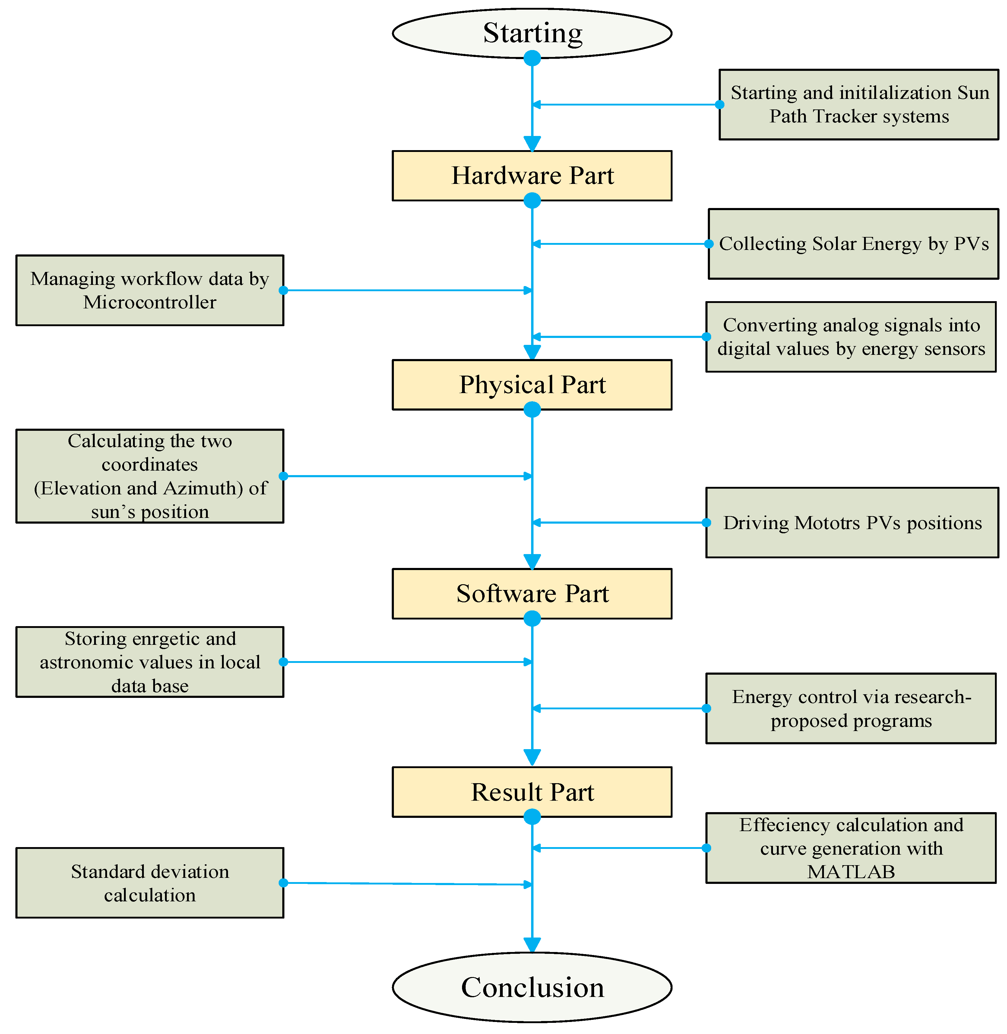
Figure 2.
Main tools of research.
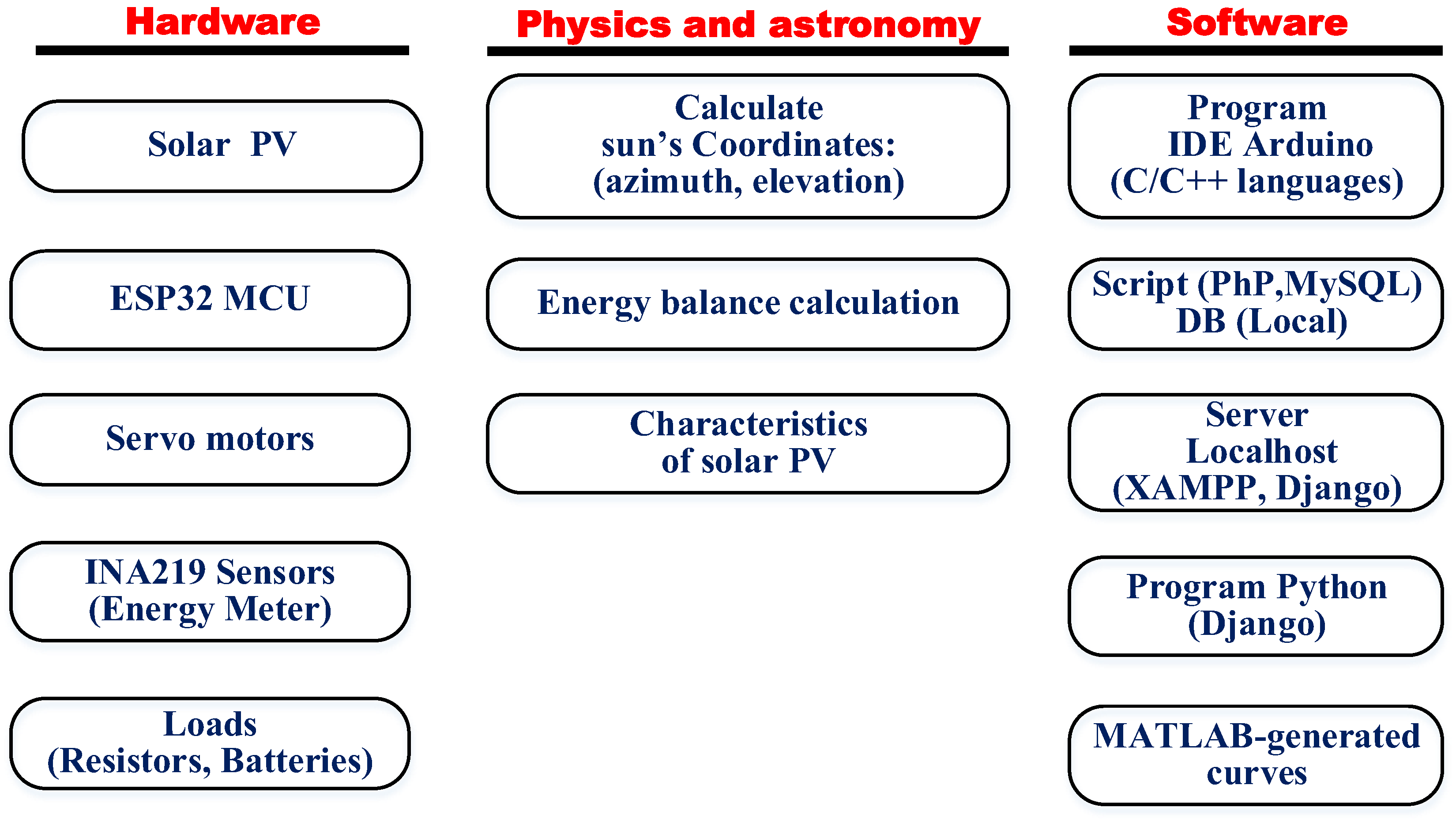
Figure 3.
Detailed functional diagram with local database of SPT.
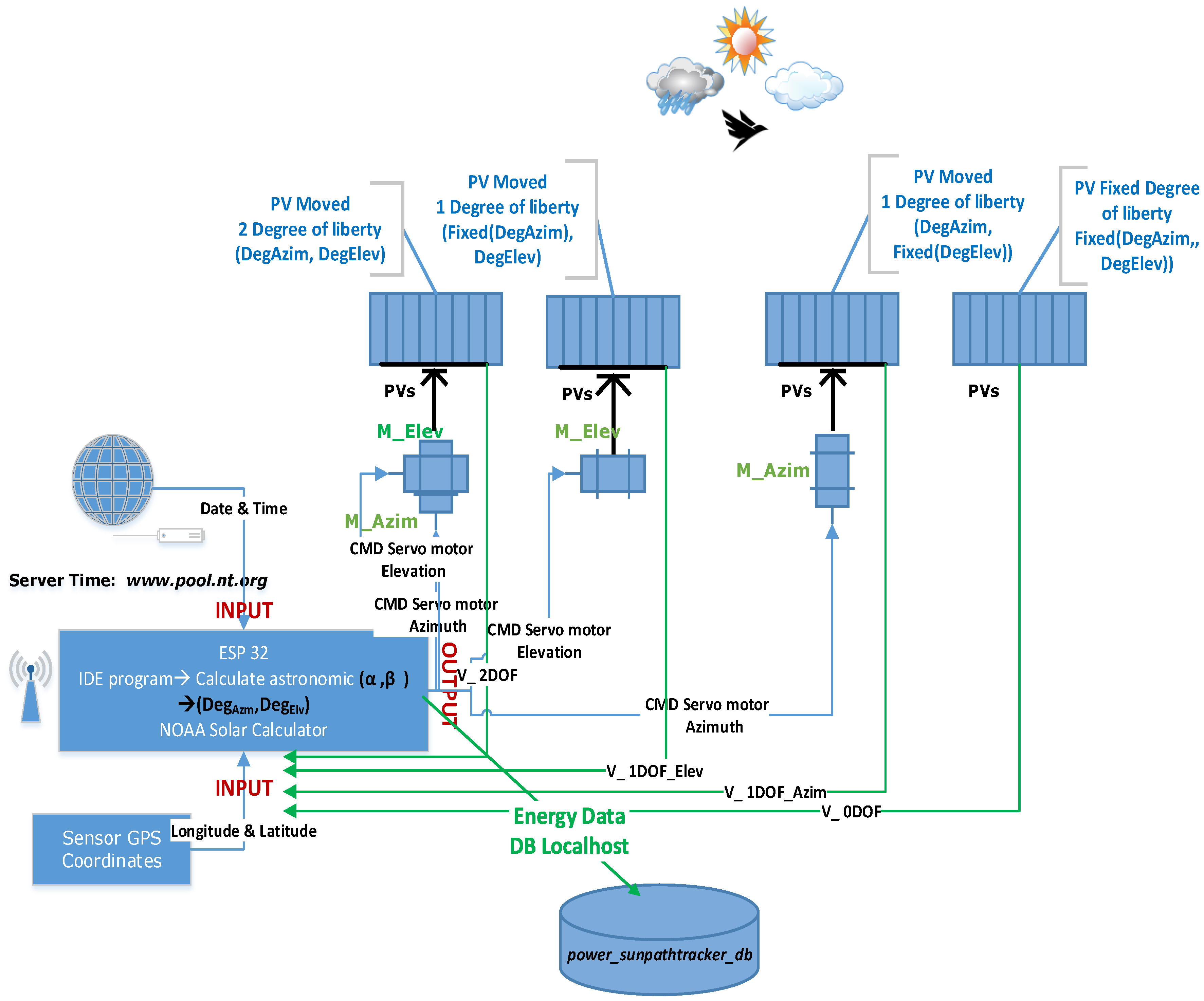
Figure 4.
Some hardware and software tools: (a) Three SPT systems and fixed PVs; (b) Local database power_sunpathtracker_db.
Figure 4.
Some hardware and software tools: (a) Three SPT systems and fixed PVs; (b) Local database power_sunpathtracker_db.
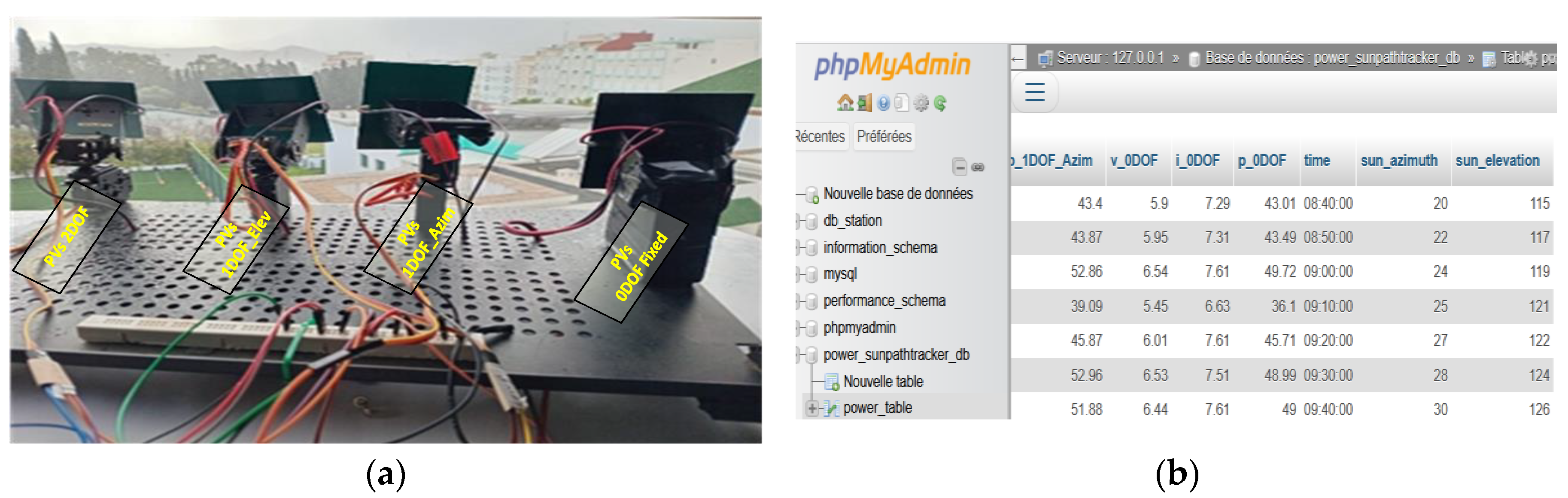
Figure 5.
Detailed electronic diagram of SPT.
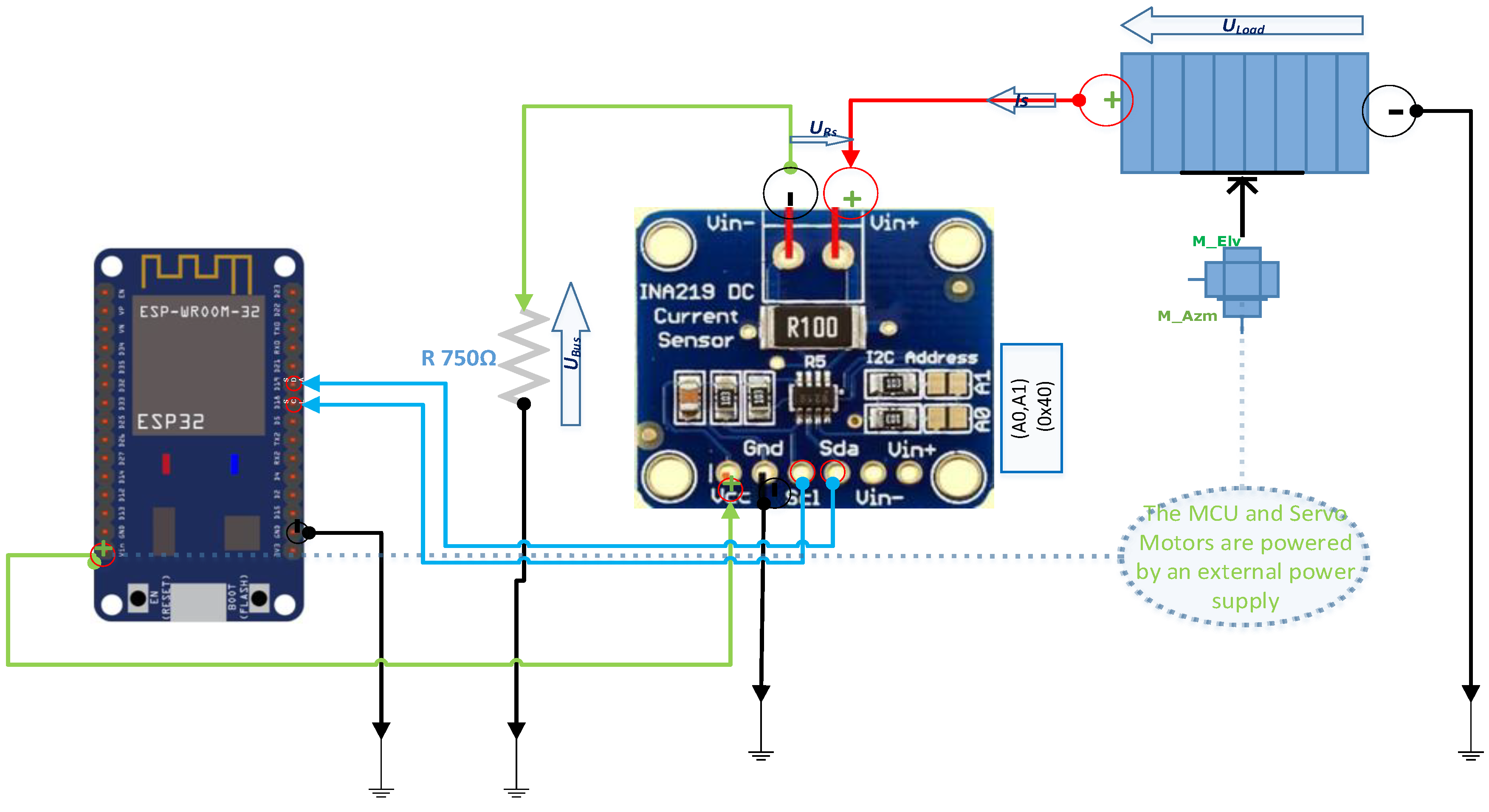
Figure 6.
Algorithm flowchart.
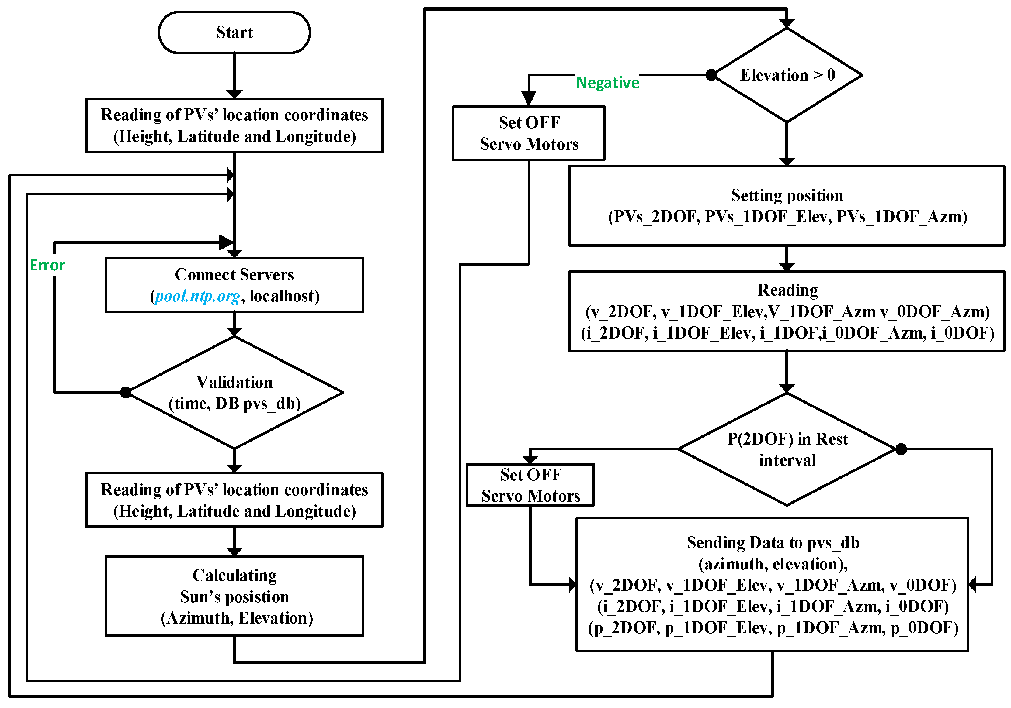
Figure 7.
Detailed electronic diagram of SPT systems.
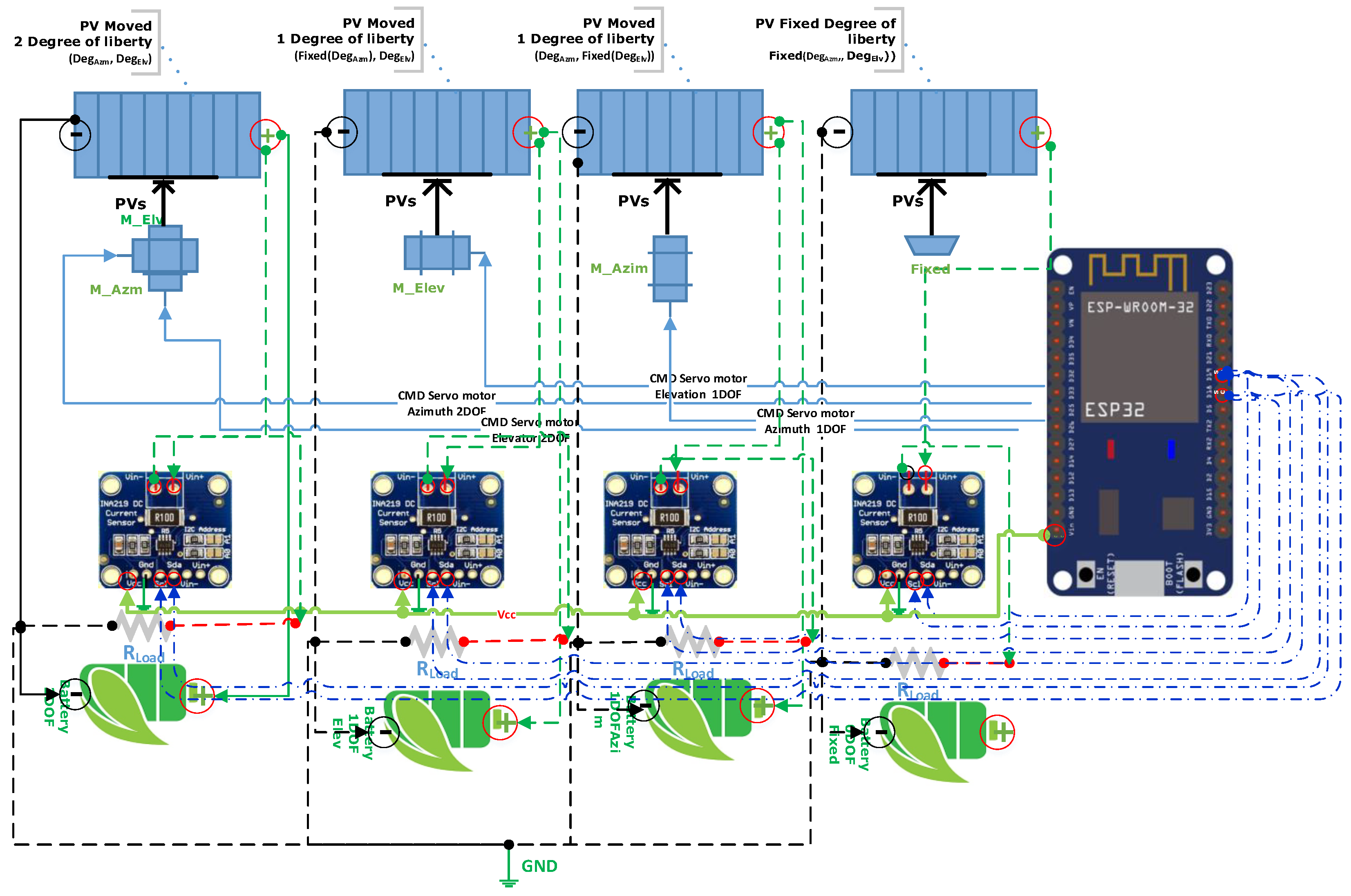
Figure 8.
Voltage evolution of the first third of the experiment day.
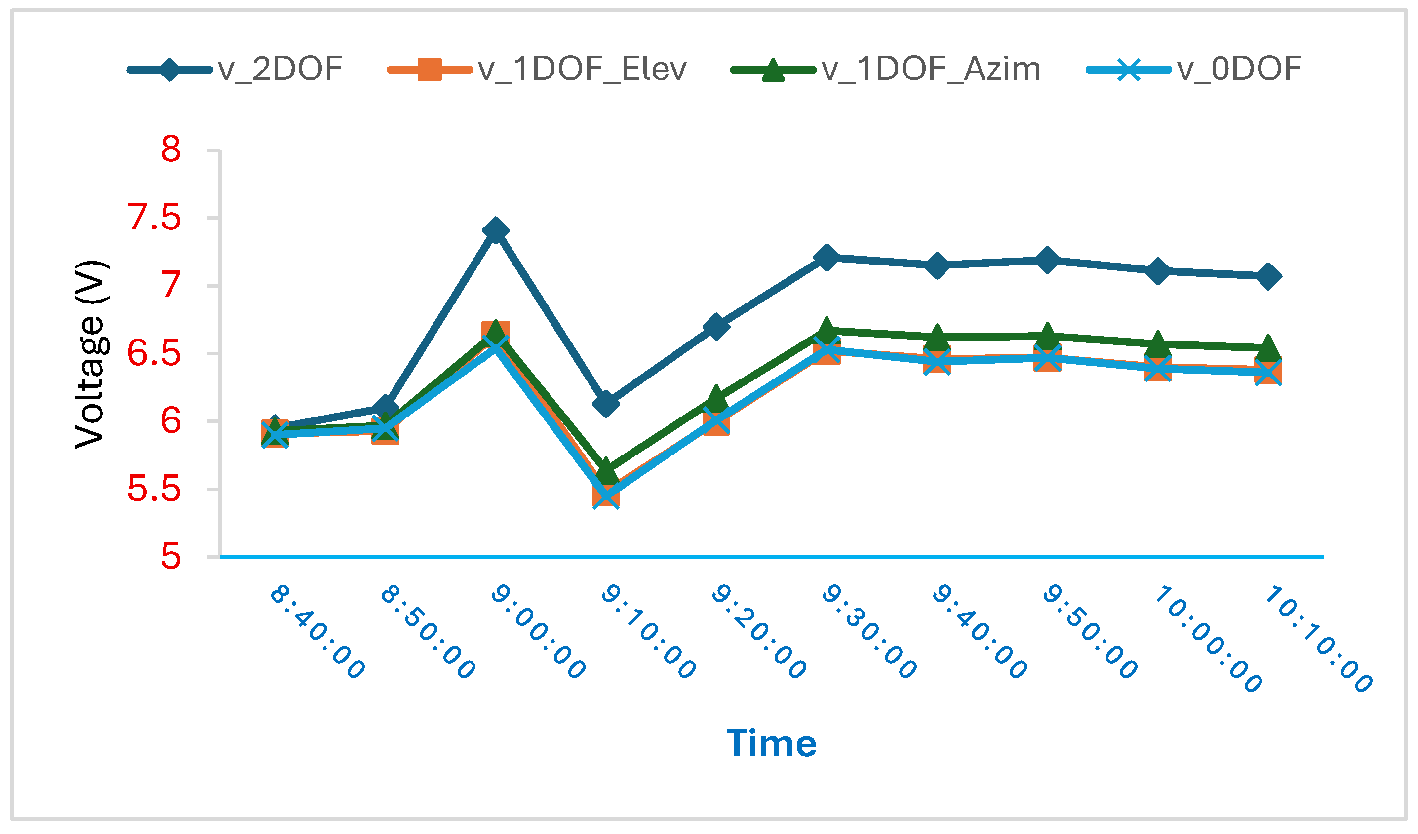
Figure 9.
Voltage evolution of the second third of the experiment day.
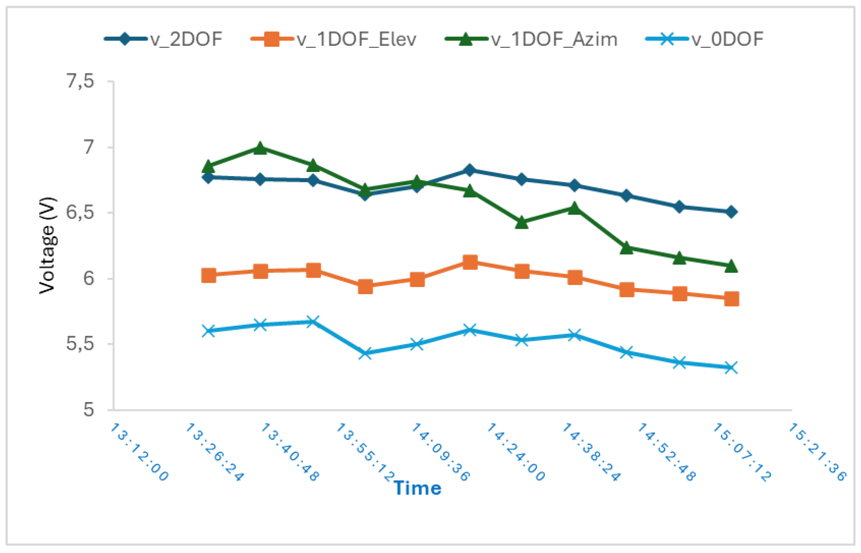
Figure 10.
Voltage evolution of the last third of the experiment day.
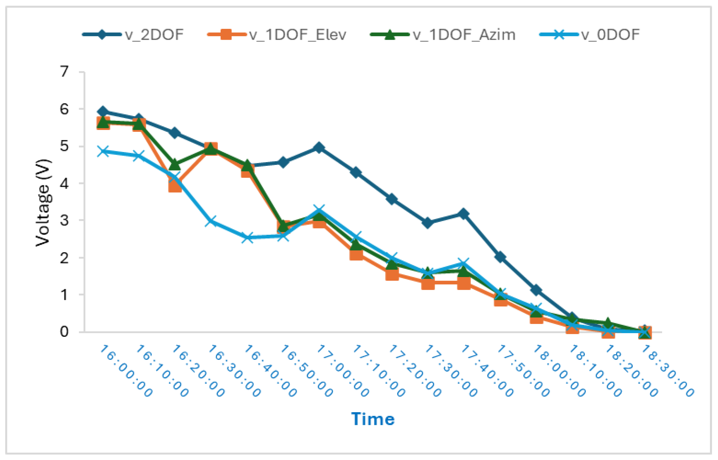
Figure 11.
Evolution of iDOF voltage throughout the whole experiment day.
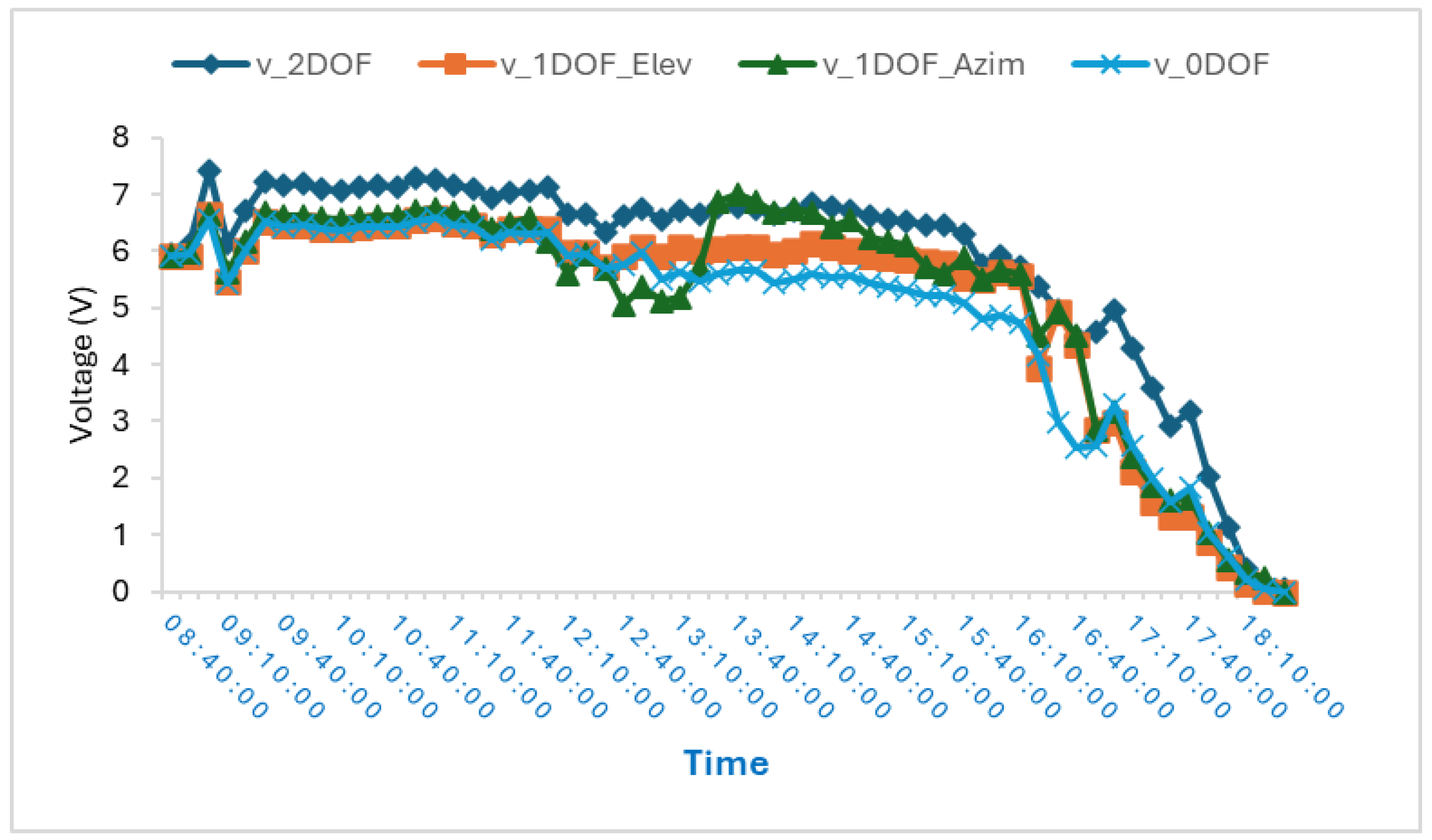
Figure 12.
Power production cycle throughout the experiment day.
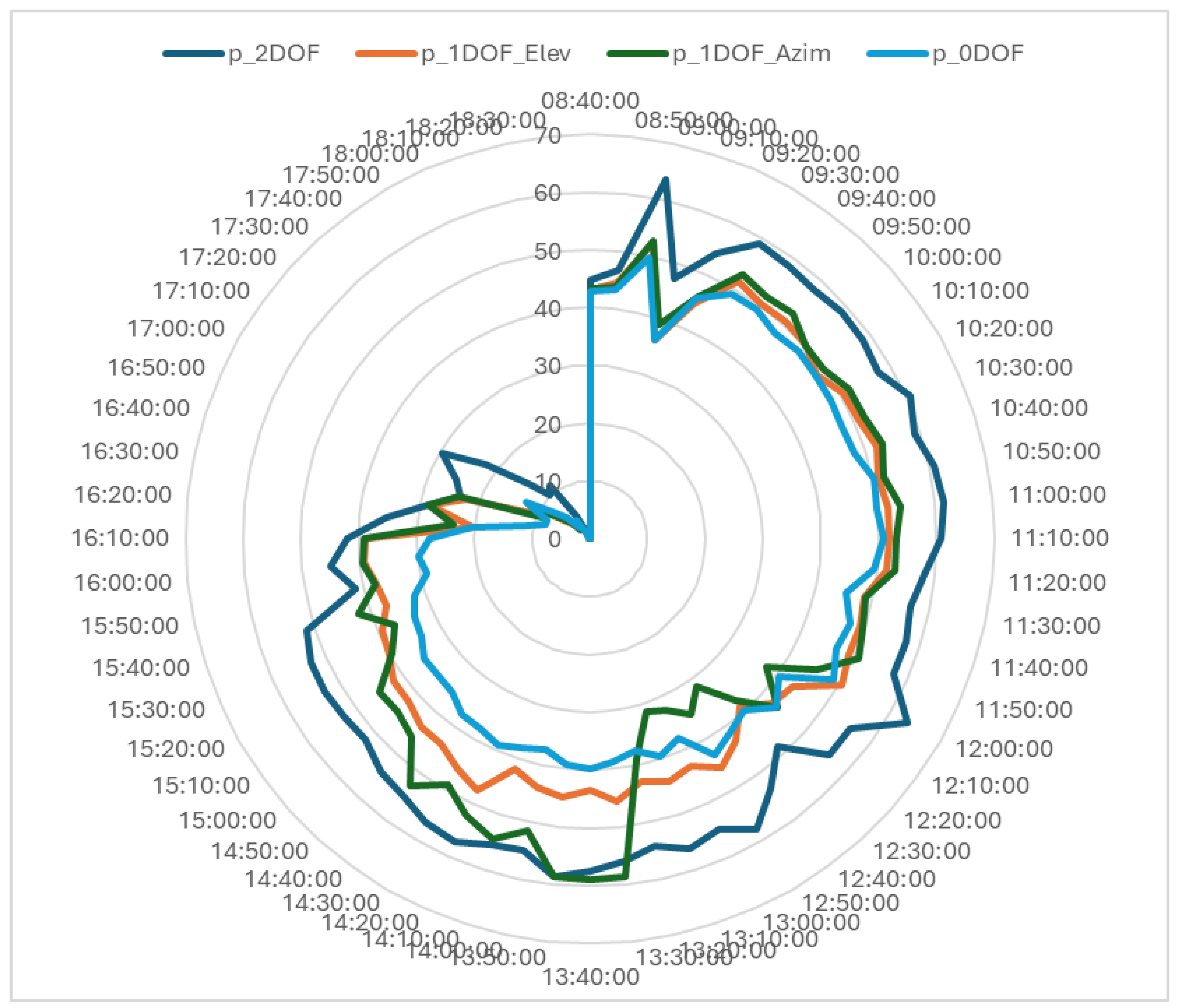
Figure 13.
Efficiency ranking of the three mobile SPTs.
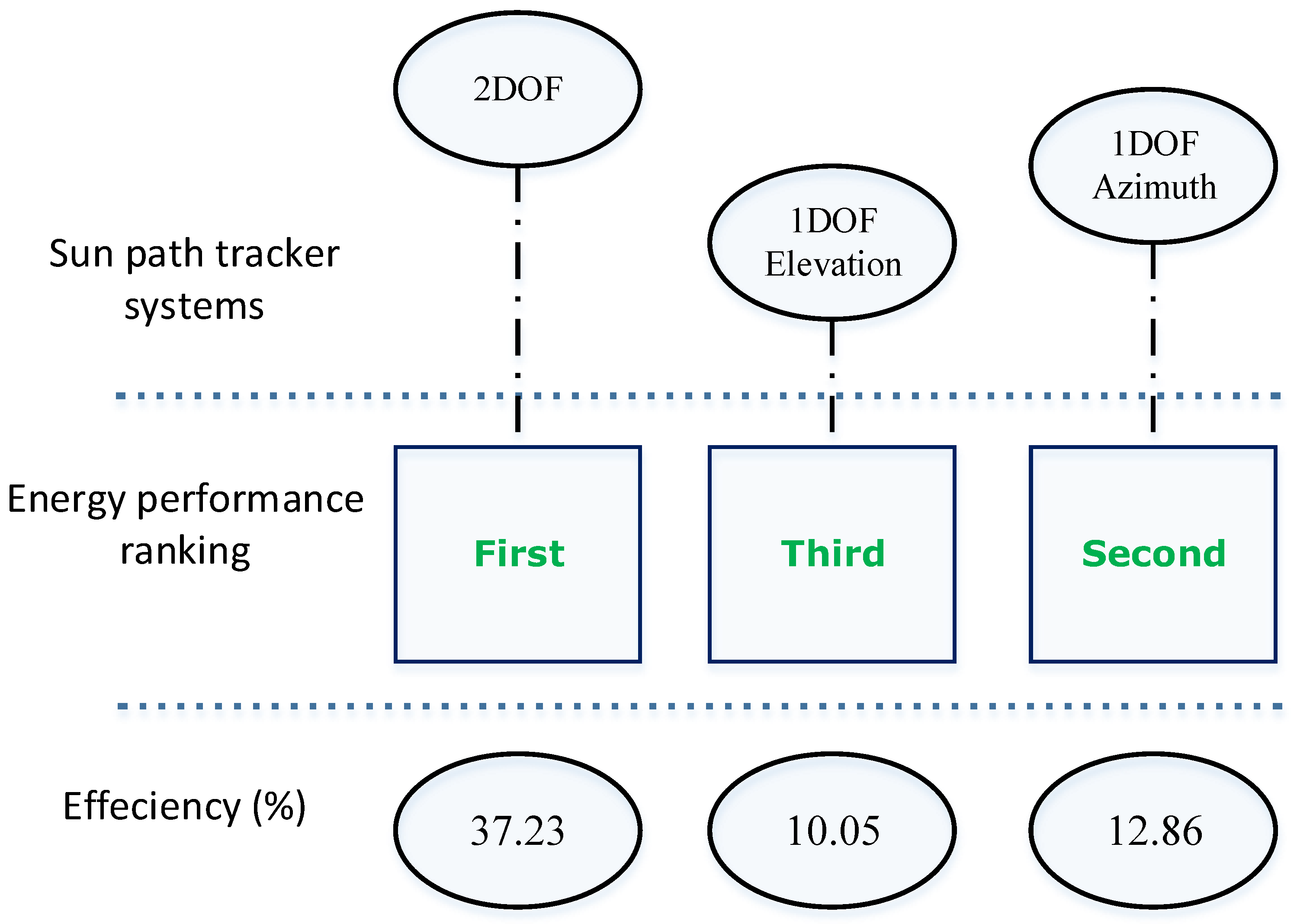
Table 1.
Inputs and outputs data parameters of sun path tracker system.
| Data Parameters | Description | |
| Inputs | Current. Voltage and Power: These PV values are obtained from the INA219 sensor and sent to the ESP32 microcontroller. | |
| Time: This time data was obtained from Server Time: www.pool.nt.organd sent to local database via Arduino IDE (Integrated Development Environment) framework and connect.ph programs. | ||
| Outputs | numerical | Cmd 2DOF_Elev: This numerical value (ADC: Analog to Digital Converter) from CPU ESP32 to command SM_Elev. |
| Cmd 2DOF_Azim: This numerical value (ADC) from CPU ESP32 to command SM_Azim. | ||
| Cmd 1DOF_Elev: This numerical value (ADC) from CPU ESP32 to command SM_Elev. | ||
| Cmd 1DOF_Azim: This numerical value (ADC) from CPU ESP32 to command SM_Azim. | ||
| astronomical | Azimuth and Elevation: These astronomical values are calculated using Equations (1) and (2), and inserted in Arduino IDE program and sent to local database, power_sunpathtracker_db, via connect.php file. | |
Table 2.
Energy characteristics of the main electronic components.
| Component | Characteristics | Energy consumption | Description | |
| Active mode | Deep mode | |||
| ESP32S2 | Power Consumption by MCU PMCU during a one cycle T is 6.37 mW | 78.32 mW | 26.85 μW | During the Ton period of active mode. the MCU consumes more energy than during the period Toff of deep mode. |
| 6.37 mW | ||||
| MG995 | n.a | 170–400 mA, 5 V | 10 mA, 5V | These typical values Stall torque: 9.8 kgf·cm (4.8V). 11 kgf·cm (6.0V). |
| Loads (Resistors) | 4x750 Ohms, ¼ W | n.a | n.a | Small carbon resistors. |
| PV Cell | 8 V, 250 mA, 2 W | n.a | n.a | Material: monocrystalline silicon cell. |
| Sensor INA219 | Analog input voltage (Min, Max) = (-26V, +26V) |
5 mW | The INA219 is a power and current shunt monitor featuring an I2C. | |
Table 3.
INA219 Binary Address (combination pins (A0, A1)).
| Sensors INA219 Indices | Two bridges stats (A0. A1) | Binary address (I2C) |
| S1→ pvs_2DOF | A0 = Bridge A1 = No Bridge |
00001 → Offset 0x41 |
| S2→ pvs_1DOF_Elev | A0 = No Bridge A1 = Bridge |
00100 → Offset 0x44 |
| S3→ pvs_1DOF_Azim | A0 = No Bridge A1 = No Bridge |
0000 → Offset 0x40 |
| S4→ pvs_0DOF | A0 = Bridge A1 = Bridge |
00101→ Offset 0x45 |
Table 4.
Energy production of different iDOF systems on March 3rd, 2025.
|
Step number |
Systems |
Voltage (V) |
Current (mA) |
Power (mW) |
Energy (kJ) |
Table 5.
Energy consumption of SPT systems.
|
MCU ESP32 mode |
SPT system |
PPVs (mW) |
PRL (mW) RL=750Ω |
PRS (mW) RS = 0.1Ω |
PMCU (mW) |
PSM (mW) |
Psens (mW) |
Ptot (mW) |
(kJ) | ||
| Deep toff | Active ton | ||||||||||
|
Total steps number: N = 60 Total experiment time: 35400 s |
26.85 (µW) |
78.32 (mW) |
2DOF | 45.7127 | 41.5874 | 0.0055 | 6.37 | Two SM | 5 | 152.9629 | 5.4148 |
| 6.37 (mW) | 100 | ||||||||||
| 1DOF_Elev | 36.6609 | 33.5619 | 0.0044 | 6.37 | One SM | 5 | 94.9363 | 3.3607 | |||
| 50 | |||||||||||
| 1DOF_Azim | 37.5973 | 33.79498 | 0.0045 | 6.37 | One SM | 5 | 95.1690 | 3.3689 | |||
| 50 | |||||||||||
| 0DOF | 33.312 | 30.26001 | 0.0040 | 6.37 | Zero SM | 5 | 41.6340 | 1.4738 | |||
| 0 | |||||||||||
Table 6.
Energy efficiency results for iDOF systems.
| µ2DOF | µ1DOF_Elev | µ1DOF_Azim | µ0DOF | time | |
| Efficiency (%) | 94.63027 | 90.55484 | 86.3928 | 92.04167 | 28/01/2025 11:43 |
| 95.62193 | 93.96307 | 89.6369 | 93.56858 | 28/01/2025 11:44 | |
| 94.23176 | 94.73339 | 88.22784 | 94.34935 | 28/01/2025 11:45 | |
| 93.57034 | 91.96778 | 88.7881 | 93.6294 | 28/01/2025 11:46 | |
| 94.30328 | 94.7538 | 89.11985 | 94.14284 | 28/01/2025 11:47 | |
| 94.68747 | 94.91592 | 88.32428 | 92.16569 | 28/01/2025 11:49 | |
| 95.81696 | 92.15889 | 89.04221 | 91.4794 | 28/01/2025 11:50 | |
| 92.35764 | 90.76984 | 87.39709 | 92.0994 | 28/01/2025 11:51 | |
| 93.62473 | 93.34688 | 91.09696 | 90.7879 | 28/01/2025 11:52 | |
| 98.42083 | 93.51257 | 90.12551 | 92.37362 | 28/01/2025 11:53 | |
| Average | 94.729 | 93.111 | 88.828 | 92.700 | Duration→ 10 min |
Table 7.
Energy Efficiency.
| time | µ2 | µ1_Elev | µ1_Azim |
| 35400 s | 37.22 % | 10.05 % | 12.86 % |
Table 9.
Standard deviation.
| 2DOF | ||
| First tier | +31.91 | Sd (%) |
| Midday | +25.29 | |
| Last tier | +53,78 |
Disclaimer/Publisher’s Note: The statements, opinions and data contained in all publications are solely those of the individual author(s) and contributor(s) and not of MDPI and/or the editor(s). MDPI and/or the editor(s) disclaim responsibility for any injury to people or property resulting from any ideas, methods, instructions or products referred to in the content. |
© 2025 by the authors. Licensee MDPI, Basel, Switzerland. This article is an open access article distributed under the terms and conditions of the Creative Commons Attribution (CC BY) license (http://creativecommons.org/licenses/by/4.0/).
Copyright: This open access article is published under a Creative Commons CC BY 4.0 license, which permit the free download, distribution, and reuse, provided that the author and preprint are cited in any reuse.


