Submitted:
03 February 2025
Posted:
04 February 2025
You are already at the latest version
Abstract
This study evaluates the performance of floating photovoltaic (FPV) systems integrated with single-axis solar tracking (FPVSAT) as an innovative approach to enhancing solar energy capture. By utilizing water bodies for solar installations, FPV systems offer a dual benefit of land conservation and improved energy efficiency due to the cooling effect of the water surface. The incorporation of single-axis solar tracking further optimizes energy generation by dynamically adjusting the panels’ orientation to follow the sun's trajectory. To analyze the system, a mathematical model was developed and validated against experimental results obtained from an FPVSAT prototype tested in Mueang District, Lop Buri, Thailand. Simulations were performed using five-minute interval weather data, with comparisons made between fixed, linear tracking, and azimuth tracking configurations. The results demonstrate that single-axis tracking systems significantly enhance solar energy yield compared to fixed installations, with the azimuth tracking configuration providing the highest efficiency. The study highlights the importance of integrating solar tracking mechanisms into FPV systems, particularly in regions with variable solar conditions, to achieve sustainable energy generation. These findings underscore the potential of FPVSAT technology as a cost-effective and efficient alternative to traditional land-based PV systems.
Keywords:
Floating photovoltaic (FPV)
; Single-axis solar tracking
; Solar energy optimization
; Renewable energy systems
; Performance analysis
1. Introduction
Global energy demand continues to rise, driven by factors such as population growth, industrialization, and technological progress. The rapid advancement of technology has led to increased energy consumption, creating two significant challenges: the depletion of fossil fuel resources and environmental degradation, including heightened CO₂ emissions and global warming. To address these issues, adopting renewable energy sources is essential for a sustainable future [1-2]. As traditional fossil fuel resources become increasingly unsustainable, both environmentally and economically, the global energy sector faces the urgent challenge of transitioning to renewable sources [3, 4]. Renewable energy technologies, including solar, wind, and hydro, are gaining traction as viable alternatives, with solar energy emerging as one of the most promising sources due to its abundance and accessibility [5]. The importance of photovoltaic (PV) technology in this transition cannot be overstated, as PV systems offer a clean, scalable, and efficient method to harness solar energy for electricity generation [6].
Photovoltaic technology directly converts sunlight into electricity without emitting greenhouse gases or pollutants during operation, aligning with the goals of sustainable energy and climate change mitigation [7]. Due to continuous advancements in efficiency and declining costs, PV systems are becoming more feasible for both large-scale and distributed power generation applications [8]. As a result, they are playing a significant role in many countries' strategies to reduce dependency on fossil fuels and decrease carbon emissions [9].
Within the spectrum of PV technologies, floating photovoltaic (FPV) systems represent an innovative solution that addresses several limitations of traditional land-based PV installations. FPV systems, installed on water bodies like lakes, reservoirs, or ponds, preserve valuable land resources that can otherwise be used for agriculture or urban development [10]. Additionally, the cooling effect of the water surface reduces the operating temperature of the PV modules, enhancing efficiency and extending their lifespan [11]. FPV systems have also been observed to reduce water evaporation and improve water quality by limiting algal growth [12], making them particularly advantageous in water-scarce regions.
Incorporating solar tracking into FPV systems presents an opportunity to further optimize energy production. Solar tracking systems, which adjust the angle of PV panels throughout the day to follow the sun’s trajectory, can significantly increase the energy yield of PV systems compared to fixed installations [13]. While dual-axis tracking systems achieve the highest levels of solar exposure, they are often complex and costly, making single-axis tracking a more practical solution for many FPV applications [14]. Single-axis trackers have demonstrated energy gains of up to 20% over fixed systems [15], which can be critical in maximizing the energy output on limited water surfaces in FPV installations [16]. Therefore, integrating solar tracking into FPV systems provides a compelling approach to further improve performance and cost-effectiveness.
Floating photovoltaic technology has emerged as an innovative approach to address land constraints and improve PV system performance. Traditionally, PV systems have been land-based, requiring significant surface area and often competing with agricultural and urban land use [17]. In contrast, FPV systems are deployed on water bodies such as lakes, reservoirs, and artificial ponds, making them suitable for regions with limited land availability. The cooling effect of water enhances the efficiency of PV modules, mitigating thermal stress and potentially prolonging module lifespan [18], [19]. Research in recent years has highlighted the operational advantages of FPV, including reduced water evaporation, improved water quality, and minimal impact on aquatic ecosystems [20]. Despite these benefits, FPV technology is still in the early stages of large-scale adoption, with a majority of installations located in countries like Japan, China, and the United States [21].
One area of significant interest in FPV systems is the incorporation of solar tracking technologies, which can further enhance energy yield. Solar tracking systems are designed to adjust the angle of PV panels relative to the sun's position, maximizing solar energy capture throughout the day. Commonly used solar tracking systems include single-axis and dual-axis trackers. Single-axis trackers follow the sun’s horizontal movement, while dual-axis trackers adjust both the horizontal and vertical angles to maintain an optimal orientation [22]. Although dual-axis trackers can achieve higher energy gains, they are generally more complex and expensive to implement, making single-axis tracking a cost-effective compromise for large-scale applications [23].
Several studies have explored the performance improvements associated with solar tracking in both land-based and floating PV systems. Single-axis tracking systems, for example, have demonstrated energy yield increases of up to 20% compared to fixed installations [24]. However, challenges remain in integrating tracking systems within FPV installations due to factors such as water surface stability, mechanical complexity, and maintenance requirements [25]. In land-based systems, tracking technologies are widely adopted in utility-scale installations where maximizing energy output justifies the added cost and complexity. In FPV applications, however, the dynamic nature of water surfaces presents unique challenges for implementing tracking mechanisms effectively [26].
Comparative studies on land-based and floating PV systems have shown that FPV installations can yield higher efficiencies under similar conditions due to the water's cooling effect [27]. When coupled with tracking capabilities, FPV systems can further enhance power generation, particularly in hot climates where temperature-induced losses are more pronounced. However, while land-based PV systems with tracking are well-established and commercially available, FPV systems with tracking are still an emerging area of research with limited deployment [28]. The complexities associated with integrating tracking in FPV systems, such as additional infrastructure costs and maintenance on water surfaces, continue to be areas of active investigation.
This study aims to analyze the performance of a floating PV system with single-axis solar tracking, contributing to a deeper understanding of FPV technology’s potential and its applicability as an efficient alternative to land-based PV systems in the renewable energy sector. This study builds on the existing literature by analyzing the performance of a floating PV system with single-axis solar tracking. By examining both theoretical and practical aspects, this research aims to contribute to the broader understanding of FPV systems with tracking technology, addressing the operational and environmental benefits that such configurations can provide.
2. Simulation and Experimental Setup
2.1. Proposed Floating PV System Configuration
The primary component of the proposed floating photovoltaic system consists of a set of tilted PV panels mounted on a floating platform equipped with a sun-tracking mechanism, as illustrated in Figure 1. One significant advantage of the floating PV system, from a sun-tracking perspective, is its ability to rotate with minimal force. This characteristic makes the system highly scalable, allowing it to be expanded into large arrays of PV panels.
The rotation of the floating PV system is achieved at a very low speed, approximately 0.25 degrees per minute, which minimizes the required energy input. This slow rotational speed enables the system to be operated using a small cable, a low-power driving motor, and minimal energy consumption. The vertical pivot axis of the system can be anchored either to a ground-fixed underwater column or a traditional anchor, providing stability and reliable sun-tracking performance.
This design highlights the scalability and energy efficiency of the proposed floating PV system, making it a practical and innovative solution for large-scale solar energy applications.
The operation of the floating PV involves rotating it by using an electric motor that pulls a cable wound around pulley ‘a’ and the cable on another side will be released by pulley ‘b’, as shown in Figure 1. These cables are connected to points set with pulleys around the pond bank and their ends are attached to a fixed point on the float (around the pyranometer shown in Figure 1). The electricity generated by the PV can be distributed on ground via an underwater cable.
The float's operation begins at 6:00 a.m., facing east, and rotates southward toward the west. From 6:00 a.m. to 6:00 p.m. (180 degree), the floating PV must be rotated for 12 hours. At night, the float rotates back to its original position (done by converting the rotating direction of motor), ready to start for the next day.
2.2. Site Location and Simulation Input Weather Data
Thailand offers exceptional solar energy potential due to its proximity to the equator, resulting in consistently high solar irradiance throughout the year. The country experiences an average of 5–6 peak sun hours per day, making it an ideal location for solar energy projects. Moreover, the increasing exploration of floating solar installations on reservoirs maximizes both energy efficiency and land use. Thailand is home to numerous deep-water reservoirs, such as dams, lakes, and large ponds, which provide suitable sites for implementing floating photovoltaic systems.
This study investigates the feasibility and performance of a floating photovoltaic system equipped with single-axis solar tracking, installed at an FPV plant located at latitude 14°02'01"N and longitude 100°43'31"E. The system was designed and its performance simulated using five-minute interval weather data obtained from the meteorological station at the Asian Institute of Technology in Bangkok, Thailand.
By utilizing detailed local meteorological data, the study provides a comprehensive evaluation of the system's efficiency and demonstrates the potential of FPV technology as an effective and sustainable alternative to traditional land-based photovoltaic systems in Thailand.
3. Mathematical Model and Validation
Solar energy availability varies by location and season due to factors such as geographical latitude, the Earth's axial tilt, day length, and local weather conditions. Regions closer to the equator benefit from more consistent solar energy, while areas at higher latitudes experience greater seasonal variation. The Earth's tilt results in changes to the angle of sunlight and day length, leading to longer, sunnier days in summer and shorter, less intense sunlight in winter. Additionally, local weather conditions, including cloud cover, humidity, and pollution, influence the amount of sunlight that reaches the Earth's surface. These variations highlight the importance of designing solar energy systems tailored to specific regional and seasonal conditions to maximize efficiency. Consequently, developing a mathematical model is crucial for conducting feasibility studies.
This study aims to evaluate how the performance of a conventional floating PV system (fixed and south-facing) can be enhanced using the proposed single-axis sun-tracking method. To estimate the solar radiation incident on the tilted PV panel surface—serving as the input energy to be converted into electricity—the 'Isotropic Sky Model,' as referenced in [29], is employed in this analysis.
3.1. Equations
To simulate both fixed and rotating (moving) tilted surfaces, it is essential to calculate all fundamental sun-Earth relationship variables, weather conditions, as well as extraterrestrial and terrestrial solar insolation. These calculations rely on input parameters, which include location-specific and weather condition data, as outlined below.
- -
- the date and watch time
- -
- the latitude angle (∅)
- -
- of site location
- -
- the tilted angle of PV-panel (β)
- -
- the azimuth angle of PV-panel (γ)
- -
- the typical annual daily terrestrial radiation (H in MJ/m2) (may using the typical meteorological year (TMY) of the site location.
Calculating the declination δ as:
where, N is the day number of the year.
Calculating the solar time (ST) as:
where, WT is watch time.
EOT is equation of time can be calculated, in minute, as:
where,
where, N is the day number of the year.
∆ is time correction factor or longitude correction (in minute) can be calculated using the local standard time meridian or longitude () and local longitude () as:
where,
Calculating the hour angle as:
where, is solar time in hours (e.g.: 10:30 = 10.5 hr or 10:45 = 10.75 hr).
Calculating the radiation falling on the tilted PV-panel surface ( in MJ/m2) using as:
where, is a constant ground reflectance or albedo of various surfaces (the value used in this study is 0.2).
is beam radiation from the sun equal to:
where, is global radiation from the sun can be calculated as:
where, a = 0.409 + 0.5016 Sin ( - 60)
b = 0.6609 - 0.4767 Sin (- 60)
and the sunrise or sunset hour angle, () is calculated from:
where, is diffuse radiation from the sky can be calculated as:
where, is daily horizontal diffuse radiation can be calculated as:
For the case that ≤ 81.4°,
For K < 0.715,
otherwise,
For the case that > 81.4°,
For K < 0.722,
otherwise,
where, the daily clearness index () can be estimated form:
where, the daily clearness index () can be estimated form:
where, the intensity of extraterrestrial radiation falling on a horizontal surface
( in J/m2) can be estimated form:
where, the value of solar constant () is 1,367 W/m2.
The geometric factor (), the ratio of the beam radiation on tilted surface to that on a horizontal surface at any time can be calculated as:
where, the cosine of incidence angle () and zenith angle () can be calculated as:
In this study, all the aforementioned equations are systematically solved and analyzed using Microsoft Excel, as in [30].
3.2. Assumptions Used in This Study
When using the ‘Isotropic Sky Model’ to estimate incident solar radiation on a tilted surface, several simplifying assumptions are made to streamline the analysis of diffuse, direct, and reflected radiation components. These assumptions include the following:
- Uniform Diffuse Radiation: The model assumes that diffuse radiation from the sky is uniformly distributed in all directions, meaning its intensity is independent of the sun’s position. This approach overlooks the fact that the sky is typically brighter near the sun.
- No Circumsolar Effect: The increased brightness near the solar disk, known as circumsolar radiation, is not accounted for in the model. Instead, diffuse radiation is treated as evenly distributed across the entire sky dome.
- Constant Reflectance (Albedo): A uniform and fixed albedo, typically ranging from 0.2 to 0.3, is assumed, representing the reflective properties of the ground surface (in this study, a water surface). This simplification assumes a constant level of reflected radiation on the tilted surface, regardless of variations in surface characteristics or seasonal changes.
- No Shading Effects: The model presumes there are no surrounding obstructions, such as trees, buildings, or other structures, that might block portions of direct or diffuse radiation.
- Fixed Tilt Angle and Elevation: It is assumed that the tilt angle and elevation of the surface remain constant for each calculation step, even though minor variations could occur due to mounting imperfections or adjustments in tracking systems.
- Ideal Atmospheric Conditions: The direct radiation component is calculated under the assumption of stable atmospheric conditions, ignoring temporary changes in air mass, aerosol concentrations, or humidity that could impact radiation levels.
- Static Solar Position Within Time Intervals: The solar position (including solar altitude and azimuth) is considered constant during each time step of the simulation, simplifying the calculation of incident angles, even though solar angles naturally change throughout the day.
These assumptions are essential for simplifying complex radiation models but may lead to slight deviations from real-world conditions.
3.3. Model Validations
To assess the accuracy of the developed mathematical model, a validation process was conducted using experimental results obtained from an actual FPVSAT prototype (as shown in Figure 2). The prototype was tested in Mueang District, Lop Buri, Thailand, located at latitude 14°46'47"N, local longitude 100°42'28"E, with a standard meridian longitude () of 105°E.
All parameters from the experimental system were used as input data for the model. For validation, the measured solar insolation incident on the PV panel surface during a clear sky day was compared with the simulation results. Solar insolation was measured and recorded using a data logger, which collected data from pyranometers installed on the FPVSAT platform and another pyranometer positioned over the water surface at the same level. The data logger was programmed to record measurements at 30-minute intervals, enabling a detailed analysis of the system's performance under real-world conditions.
4. Results and Discussion
In this theoretical study, the performance of an FPV system is evaluated and compared across three distinct configurations, as described below:
- Fixed Configuration: In this setup, the PV panels are tilted at an angle equal to the site latitude and mounted on a consolidated floater without any sun-tracking mechanism.
- Linear Tracking Configuration: The PV panels are tilted at the site latitude and mounted on a consolidated floater. The entire system rotates horizontally from -90° (east) to +90° (west) at a constant rotation speed.
- As sun Azimuth Tracking Configuration: In this configuration, the PV panels are tilted at the site latitude, mounted on a consolidated floater, and continuously rotated in real-time to align directly with the solar azimuth angle.
One notable advantage of using floaters on a water surface is their ease of rotation, which requires minimal force and a simple mechanism. However, between the "linear tracking" and "solar azimuth tracking" configurations, the linear tracking method is simpler and more cost-effective, making it a practical choice for implementation despite offering slightly lower performance compared to the solar azimuth tracking configuration.
4.1. Model Validations
To validate the developed model, the results of the simulation were compared with the experimental results obtained from the experimental setup shown in Figure 2. A mention in [29,30], the daytime from 6:00 AM to 6:00 PM should be focused. As mentioned in the assumption section, the experimental results of a very clear sky must be chosen and taken for model validation. Simulation results on the solar radiation profiles of two cases: fixed and single axis solar tracking, were compared with the measured values (on May 1st, 2024) as shown in as shown in Figure 3. The validation results show that the simulation results agree well with the experimental results.
4.2. Performance Analysis
To analyze the daily performance of the proposed FPVSAT, the mean day of the month mentioned in [26], as shown in Table 1, are used as input parameter.
To analyze the daily performance of the proposed FPVSAT, the mean day of the month are used as input parameter. Figure 4 shows the total solar radiation on the mean day of all months. As an example of the daily performance, the simulatiuon result on July 17th is used for discussion. The comparison among three cases: ‘Fixed’ (blue line), ‘Linear tracking’ (red line) and ‘as solar azimuth’ (green line) is discussed. The results demonstrate that early in the day (6:00–8:00 AM) and late in the afternoon (4:00–6:00 PM), both tracking systems ('Linear tracking' and 'as solar azimuth') outperform the fixed system, with the 'as solar azimuth' setup showing a slight edge due to its azimuthal alignment. Around noon, where solar radiation is at its peak, the difference between the three systems is less pronounced. However, the 'as solar azimuth' system still demonstrates a higher efficiency, reflecting its better angular alignment with the sun. The solar radiation for the fixed system exhibits the lowest values throughout the day (3.86 kWh/m2/day), as expected, due to its inability to adjust its position relative to the sun's movement. The linear tracking system significantly improves solar radiation capture (4.18 kWh/m2/day), especially during mid-morning and mid-afternoon, where its alignment with the sun's position allows for greater efficiency compared to the fixed system. The 'as solar azimuth' case, represented by the green line, demonstrates the highest solar radiation values overall (4.24 kWh/m2/day), particularly during the peak hours. This method appears to provide the closest alignment with the sun's path, maximizing the capture of solar radiation.
Figure 5 shows the monthly average daily solar energy over year. The fixed system consistently has the lowest daily incident radiation throughout the year. While it shows a seasonal variation pattern (highest in winter and lowest in rainy days), its inability to adjust to the sun's position limits its effectiveness, particularly during periods of low solar altitude. Linear tracking provides a notable improvement over the fixed system, especially in months with longer daylight hours, as it adjusts the panel's position to align better with the sun. However, its performance is still slightly inferior to the 'as solar azimuth' system, particularly during summer when azimuth alignment further optimizes energy capture. This system outperforms the other two throughout the year, maintaining higher daily incident radiation levels due to its ability to follow the sun's azimuth angle accurately. The improvement is most significant during periods with high solar angles, demonstrating its superior efficiency.
Based on the yearly solar energy calculations, the fixed system achieves 1.41 MWh/m²/year, while the linear tracking system shows an 8.2% improvement with 1.53 MWh/m²/year. The 'as solar azimuth' system provides the highest annual yield at 1.55 MWh/m²/year, representing a 9.8% increase over the fixed system and a marginal 1.4% gain over the linear tracking system. Despite the slight improvement in linear tracking, the 'as solar azimuth' system remains the most efficient option for maximizing energy output.
4.3. Influences of Latitude on the FPVSAT Performance
To analyze the influences of location at any latitude angle on the performance of the proposed FPVSAT, the mean days of the month are used as input parameter. The variation of latitude angle from the equator to 60 (High Latitude) degrees is used for simulation. Figure 6 shows the Daily solar energy of all mean days over year at latitude angle of 0° (Equator), 14.78° (Tropical Zone), 30° (Subtropical Zone) and 45° (Temperate Zone). In addition, the simulation results of higher latitude are in the same trend.
As latitude increases from the equator to 60°, the overall daily incident solar radiation decreases for fixed solar panels but increases significantly for systems utilizing linear and azimuth tracking. Fixed systems show consistent but lower solar energy output across all latitudes. Linear tracking and azimuth tracking systems provide significantly higher energy yields, especially at higher latitudes. At higher latitudes (e.g., 45° and 60°), the seasonal variation in solar energy is much more pronounced compared to regions closer to the equator. At higher latitudes show lower energy outputs for fixed systems, whereas ‘as sun azimuth tracking’ systems maintain relatively higher performance, but very close to ‘linear tracking’ system.
Figure 7 shows the simulation results of the influences of latitude angle on the daily total radiation. At the Equator, the values of total radiation are consistent at 3.74 kWh/m²/day across fixed, linear, and azimuth tracking systems, with no significant improvement from tracking mechanisms. Mean that tracking systems do not provide any benefit at the equator due to the high and consistent solar angles throughout the year.
In tropical zone, fixed systems produce 3.86 kWh/m²/day, while linear tracking achieves 4.18 kWh/m²/day (+8.21%), and azimuth tracking yields 4.24 kWh/m²/day (+9.75%). Tracking systems show a slight advantage, making them viable for marginal energy gains in tropical regions with moderate seasonal variation.
For subtropical zone (around 30° of latitude), daily total radiation of fixed systems yields 4.42 kWh/m²/day, while linear tracking improves to 5.29 kWh/m²/day (+19.79%), and azimuth tracking produces 5.36 kWh/m²/day (+21.35%). Tracking systems annually provide significant energy gains, highlighting their value in subtropical zones where sun angles vary more over the year.
At the location around the temperate zone (about 45° of latitude), Fixed systems generate 5.83 kWh/m²/day, while linear tracking increases this to 7.63 kWh/m²/day (+31.02%), and azimuth tracking provides 7.67 kWh/m²/day (+31.61%). While tracking systems outperform fixed ones significantly, showcasing their importance in temperate regions with pronounced seasonal variability.
For the location at high latitudes, fixed systems provide 13.00 kWh/m²/day, whereas linear tracking achieves 17.42 kWh/m²/day (+34.02%), and azimuth tracking yields 17.40 kWh/m²/day (+33.91%). Tracking systems exhibit substantial gains, making them indispensable for maintaining energy production in regions with extreme seasonal variation and low solar angles.
5. Conclusions
This study highlights the critical role of geographic location and solar tracking technologies in optimizing the performance of solar energy systems. The findings emphasize that fixed systems FPV, while the least efficient, are suitable for equatorial regions (latitude 0°) due to consistent solar availability and minimal seasonal variations. They offer stable but limited energy input and are a cost-effective option for budget-sensitive projects. Single-axis sun-tracking systems significantly outperform fixed systems, achieving an average annual solar energy increase of 9.75%. Tracking along sun azimuth systems deliver the highest energy yields, making them ideal for maximizing energy production in temperate and high-latitude regions (30°–60°). Linear tracking systems offer a practical balance between energy yield and system complexity, making them a cost-effective alternative to azimuth tracking systems.
At higher latitudes, the effectiveness of fixed systems diminishes due to lower solar angles and pronounced seasonal variations. Solar tracking systems, particularly azimuth tracking, effectively address these challenges, ensuring year-round energy efficiency and reliability. For equatorial and tropical zones, fixed systems may suffice due to stable solar angles. For temperate and high-latitude regions, adopting tracking technologies is essential to optimize solar energy output and address seasonal variability.
The implementation of location-specific designs and strategic investments in solar tracking technologies is crucial to harness the full potential of solar energy. Between linear and azimuth tracking systems, linear tracking is more practical for actual implementation due to its simpler mechanism and cost-effectiveness, despite slightly lower performance compared to azimuth tracking. This research underscores the importance of adopting solar energy systems tailored to regional characteristics to achieve long-term sustainability and maximize energy yield.
Author Contributions
Conceptualization, B.P.; methodology, B.P. and C.P.; software, C.P. and P.C.; validation, B.P. and P.C.; formal analysis, P.C. and B.P.; writing—original draft preparation, B.P.; review and editing, B.P. and P.C.; visualization, C.P. and P.C.; supervision, B.P. and C.P.; investigation, B.P.; resources, C.P. and B.P. All authors have read and agreed to the published version of the manuscript.
Funding
This research paper publication was supported by Rajamangala University of Technology Thanyaburi (RMUTT) towards the Department of Mechanical Engineering at the Faculty of Engineering, RMUTT, Thailand with no external funding attached to it.
Data Availability Statement
The data collection was obtained from global solar atlas database potential, renewable energy outlook in Thailand, and Solargis website.
Acknowledgments
The authors wish to thank Rajamangala University of Technology Thanyaburi (RMUTT) for providing financial support for his research and publications.
Conflicts of Interest
The authors declared no conflict of interest in this research paper.
Abbreviations
The following abbreviations, symbols and parameters with appropriate subscripts and superscripts are used in this manuscript:
| EOT | Equation of Time (minutes) |
| FPV | Floating Photovoltaic |
| FPVSAT | Floating Photovoltaic System with Single-Axis Solar Tracking |
| H | Total daily terrestrial solar radiation (MJ/m²) |
| Hd | Daily horizontal diffuse radiation (MJ/m²) |
| H0 | Extraterrestrial solar radiation (MJ/m²) |
| I | Global radiation from the sun (MJ/m²) |
| Ib | Beam radiation from the sun (MJ/m²) |
| Id | Diffuse radiation from the sky (MJ/m²) |
| Isc | Solar Constant (1,3671,3671,367 W/m²) |
| IT | Solar radiation incident on the tilted PV panel surface (MJ/m²) |
| Llo | Local longitude (degrees) |
| Lst | Standard meridian longitude (degrees) |
| N | Day number of the year |
| PV | Photovoltaic |
| Rb | Ratio of beam radiation on tilted surface to horizontal surface) |
| ST | Solar Time (hour) |
| TMY | Typical Meteorological Year |
| WT | Watch Time |
| ∅ | Latitude angle of the site location |
| β | Tilt angle of the PV panel |
| γ | Azimuth angle of the PV panel |
| Time correction factor or longitude correction (minute) | |
| θ | Incidence angle of solar radiation (degrees) |
| ρ | Surface reflectance or albedo (dimensionless) |
| θz | Zenith angle of solar radiation (degrees) |
| ω | Hour angle (degrees) |
| ωs | Sunrise or sunset hour angle (degrees) |
| δ | Solar declination angle (degrees) |
| K | Daily clearness index (dimensionless) |
References
- Prasartkaew, B.; Ngernplabpla, A. Investigation on the Performance of a Paraboloids Heliostat for Concentrated Central Receiver Solar Collector. In Proceedings of the 6th International Conference on Science, Technology and Innovation for Sustainable Well-Being (STISWB VI), Siem Reap, Cambodia; 2014. [Google Scholar]
- Prasartkaew, B.; Sukpancharoen, S. An Experimental Investigation on a Novel Direct-Fired Porous Boiler for Low-Pressure Steam Applications. Case Studies in Thermal Engineering 2021, 26, 101169. [Google Scholar] [CrossRef]
- International Energy Agency. World Energy Outlook 2021; IEA Publications: Paris, France, 2021. [Google Scholar]
- Prasartkaew, B.; Kumar, S. Design of a renewable energy based air-conditioning system. Energy and buildings 2014, 68, 156–164. [Google Scholar] [CrossRef]
- United Nations Environment Programme. Emissions Gap Report 2020; UNEP Publications, 2020. [Google Scholar]
- Lewis, N.S.; Nocera, D.G. Powering the planet: Chemical challenges in solar energy utilization. Proc. Natl. Acad. Sci. USA 2006, 103, 15729–15735. [Google Scholar] [CrossRef]
- Fthenakis, V.M. Sustainability of photovoltaics: The case for thin-film solar cells. Renew. Sustain. Energy Rev. 2009, 13, 2746–2750. [Google Scholar] [CrossRef]
- Fraunhofer Institute for Solar Energy Systems. Photovoltaics report. Fraunhofer ISE. 2020. Available online: https://www.ise.fraunhofer.de.
- Intergovernmental Panel on Climate Change, Global Warming of 1.5°C. IPCC, 2018.
- Choi, Y.; Lee, K.; Kim, H. A study on power generation analysis of floating PV system considering environmental impact. Environ. Sci. Technol. 2014, 48, 13125–13132. [Google Scholar] [CrossRef]
- Liu, H.; Wang, Z.; He, W. Evaluation of floating photovoltaic systems’ cooling effect on photovoltaic panels. J. Renewable Energy 2017, 21, 319–328. [Google Scholar]
- Chatterjee, S.; Chatterjee, A. Types and benefits of solar tracking systems in photovoltaic applications. Renewable Energy Rep. 2019, 24, 45–54. [Google Scholar]
- Kacira, M. Analysis of single-axis and dual-axis tracking PV systems: Efficiency and cost implications. Sol. Energy 2016, 134, 14–23. [Google Scholar]
- Sanchez, J.; Batlles, F.J. Performance analysis of single-axis tracking PV systems: A case study. Energy Convers. Manag. 2019, 182, 46–58. [Google Scholar]
- Mizuno, T. Performance improvements in floating solar plants with tracking mechanisms. Int. J. Photovoltaic Syst. 2017, 6, 110–115. [Google Scholar]
- Choi, J.; Lee, K.; Kim, H. A study on power generation analysis of floating PV system considering environmental impact. Environ. Sci. Technol. 2014, 48, 13125–13132. [Google Scholar] [CrossRef]
- Liu, H.; Wang, Z.; He, W. Evaluation of floating photovoltaic systems’ cooling effect on photovoltaic panels. J. Renewable Energy 2017, 21, 319–328. [Google Scholar]
- Liu, H.Z.; Li, C.T.; Zhang, J.W. Environmental benefits of floating PV on artificial water bodies. Energy Rep. 2020, 6, 1216–1222. [Google Scholar]
- Smith, R.; Jones, L. Global adoption trends in floating photovoltaic systems. Int. J. Renewable Energy 2019, 23, 1–9. [Google Scholar]
- Chatterjee, S.; Chatterjee, A. Types and benefits of solar tracking systems in photovoltaic applications. Renewable Energy Rep. 2019, 24, 45–54. [Google Scholar]
- Kacira, M. Analysis of single-axis and dual-axis tracking PV systems: Efficiency and cost implications. Sol. Energy 2016, 134, 14–23. [Google Scholar]
- Sanchez, J.; Batlles, F.J. Performance analysis of single-axis tracking PV systems: A case study. Energy Convers. Manag. 2019, 182, 46–58. [Google Scholar]
- Mizuno, T. Performance improvements in floating solar plants with tracking mechanisms. Int. J. Photovoltaic Syst. 2017, 6, 110–115. [Google Scholar]
- Wang, L.; Zhao, Q.; Zhou, X. Challenges and advancements in tracking mechanisms for FPV systems. IEEE Trans. Sustain. Energy 2020, 11, 486–493. [Google Scholar]
- Patel, N.; Kumar, P. Comparative analysis of land-based and floating PV systems under varying environmental conditions. Renewable Energy J. 2021, 29, 204–210. [Google Scholar]
- Gomez, F.; Torres, R. Opportunities and challenges in integrating tracking with floating PV systems. Solar Photovoltaic Res. 2018, 31, 93–101. [Google Scholar]
- Prasartkaew, B.; Kumar, S. Experimental study on the performance of a solar-biomass hybrid air-conditioning system. Renewable Energy 2013, 57, 86–93. [Google Scholar] [CrossRef]
- Prasartkaew, B.; Kumar, S. A low carbon cooling system using renewable energy resources and technologies. Energy and Buildings 2010, 42, 1453–1462. [Google Scholar] [CrossRef]
- Duffie, J.A.; Beckman, W.A.; Blair, N. Solar engineering of thermal processes, photovoltaics and wind; John Wiley & Sons, 2020. [Google Scholar]
- Prasartkaew, B. Mathematical modeling of an absorption chiller system energized by a hybrid thermal system: Model validation. Energy Procedia 2013, 34, 159–172. [Google Scholar] [CrossRef]
Figure 1.
Proposed floating PV and sun tracking mechanism.
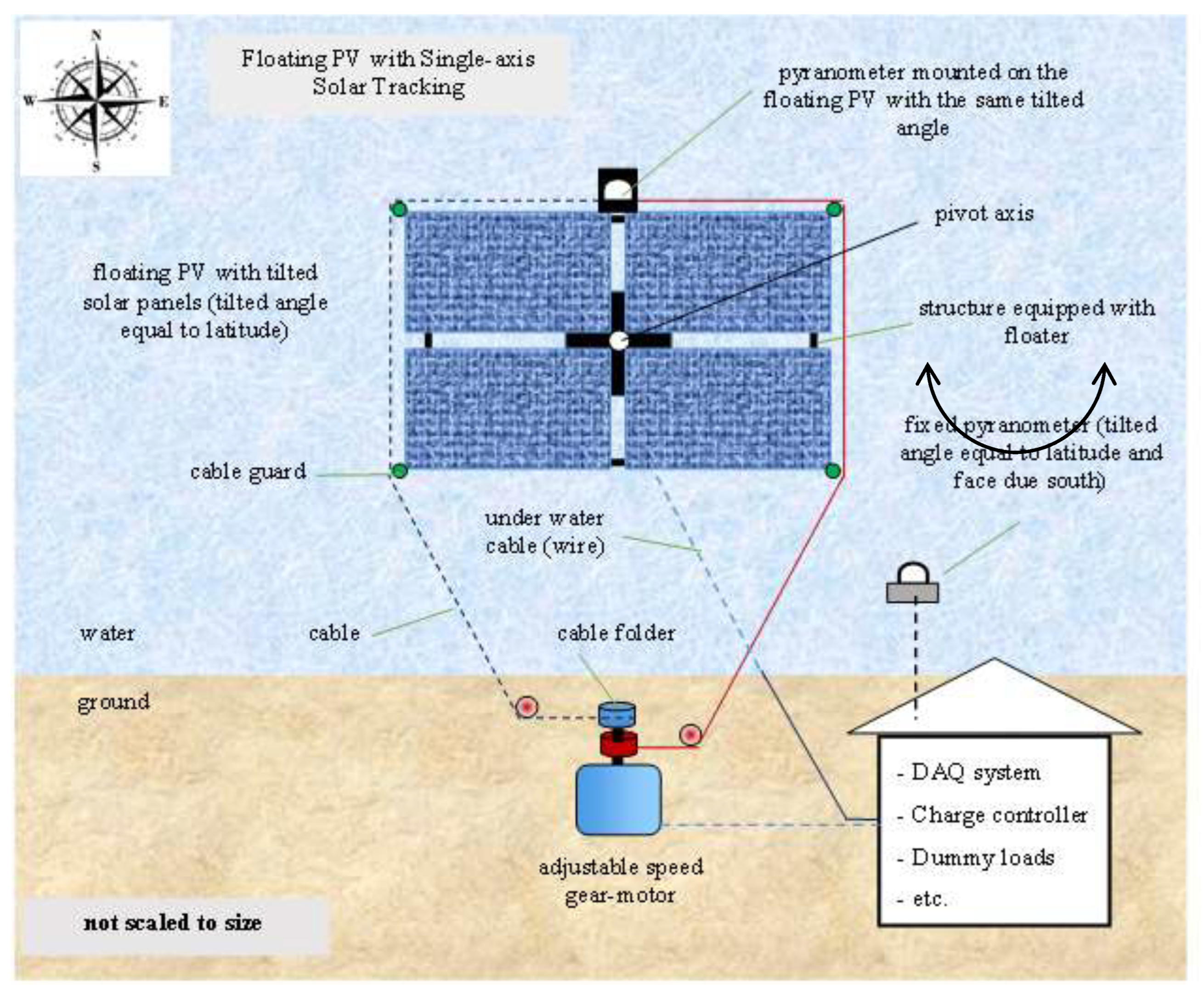
Figure 2.
A prototype floating PV used for model validation. (a) Experimental setup at the test site; (b) Drawing of FPVSAT used in this study.
Figure 2.
A prototype floating PV used for model validation. (a) Experimental setup at the test site; (b) Drawing of FPVSAT used in this study.
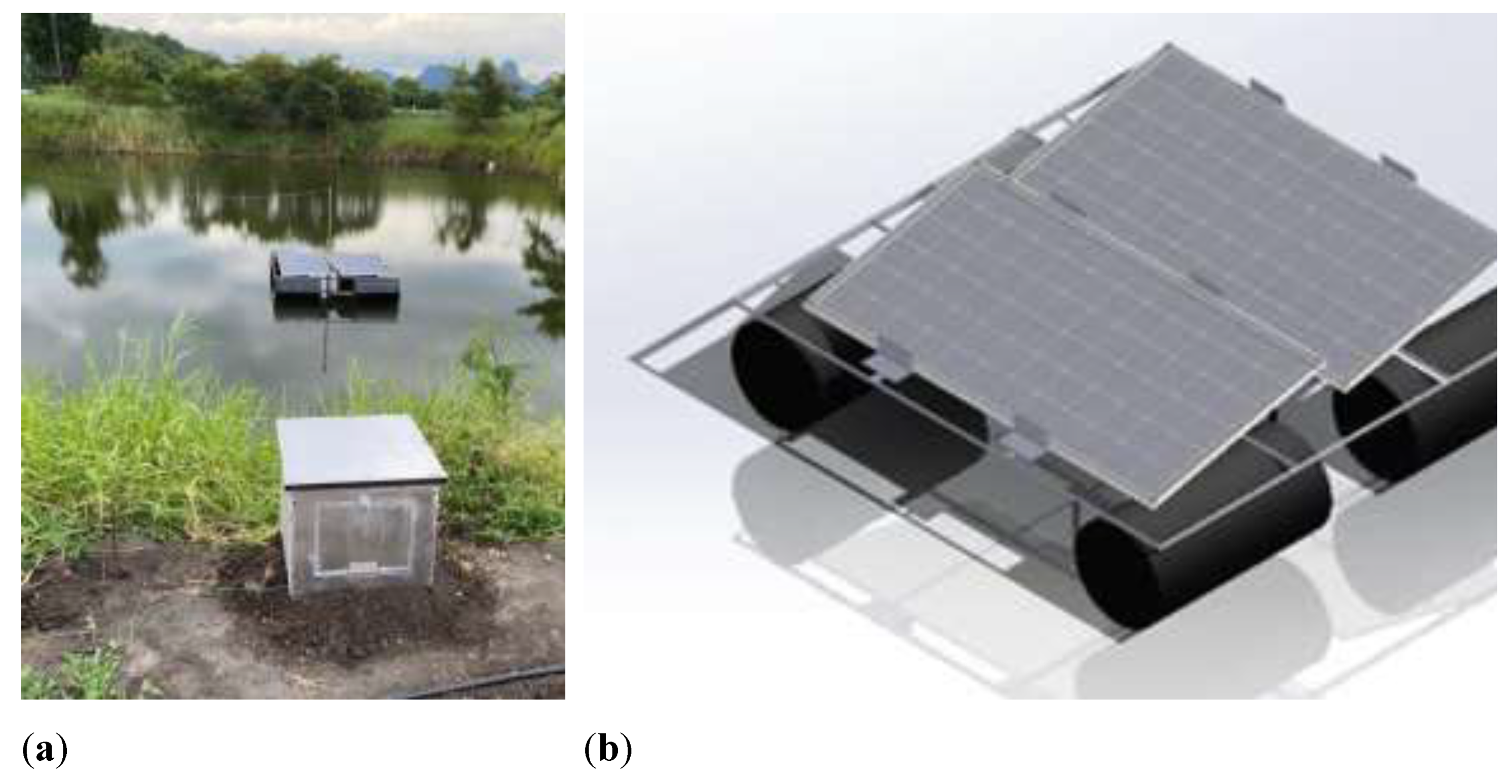
Figure 3.
Validation of the model through a comparison of simulation results with experimental data.
Figure 3.
Validation of the model through a comparison of simulation results with experimental data.
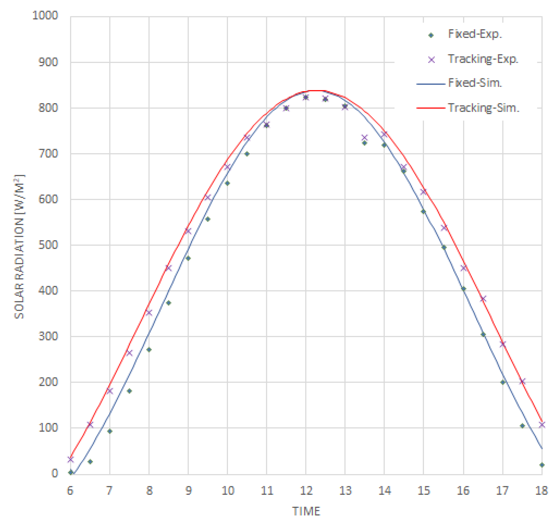
Figure 4.
Total solar radiation on the mean day of all months at = 14°46'47"N, = 100°42'28"E.
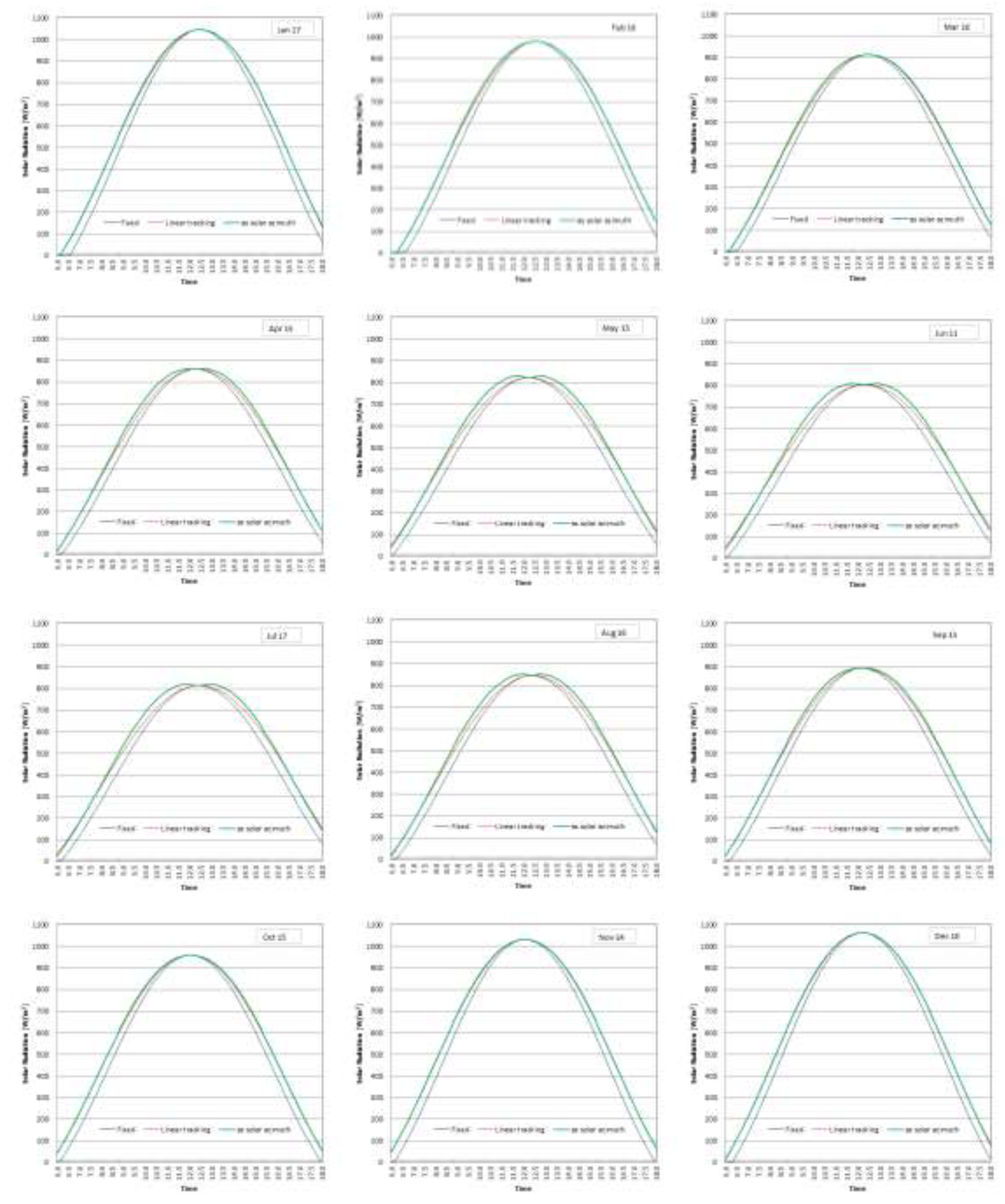
Figure 5.
Daily solar energy of all mean days over year at = 14°46'47"N, = 100°42'28"E.
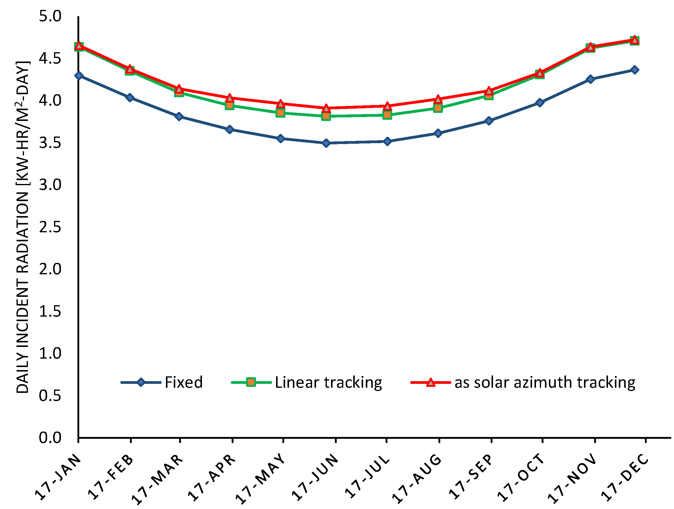
Figure 6.
Daily solar energy of all mean days over year at latitude angle of 0, 14.78, 30 and 45°.
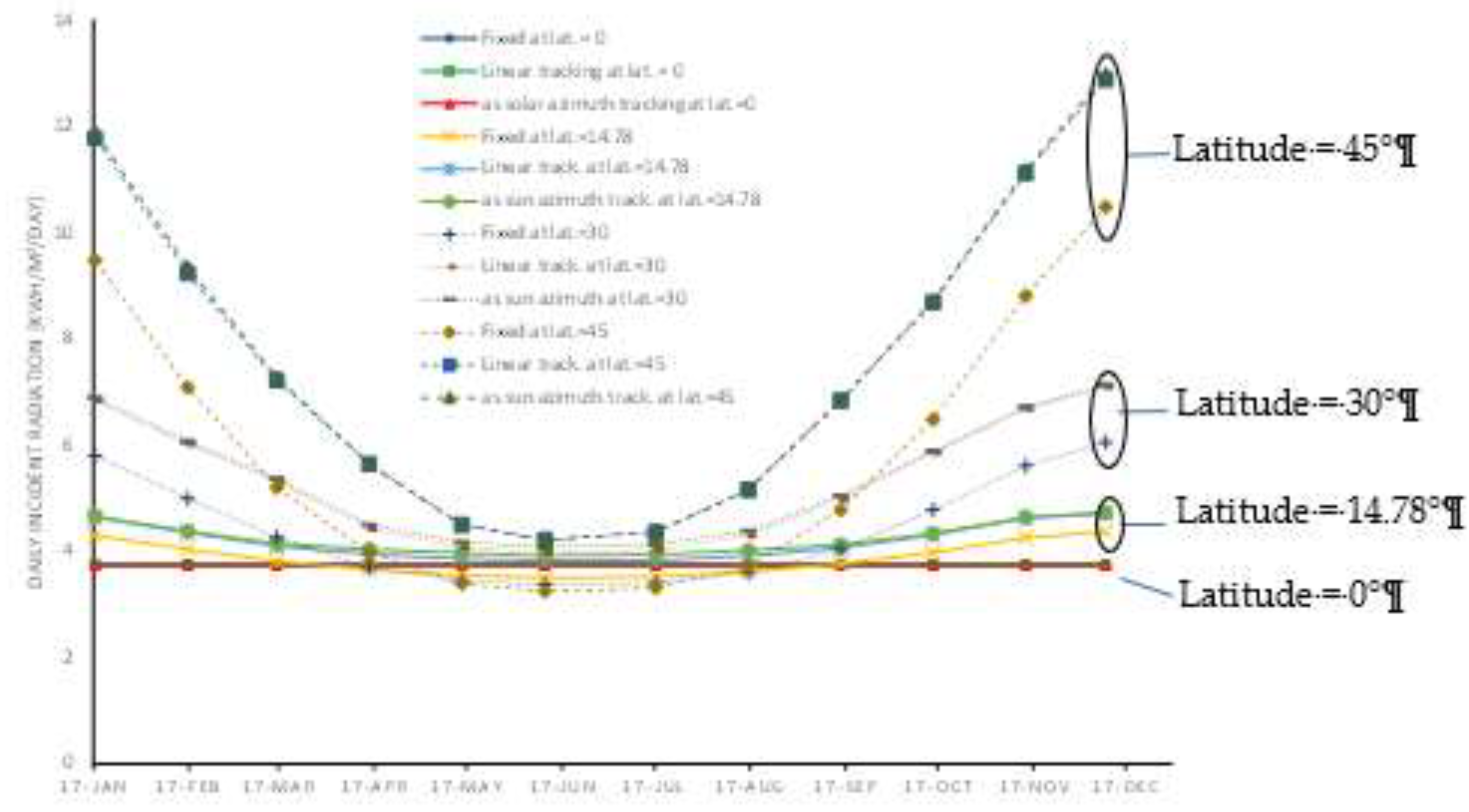
Figure 7.
Influences of latitude angle on the daily total radiation.
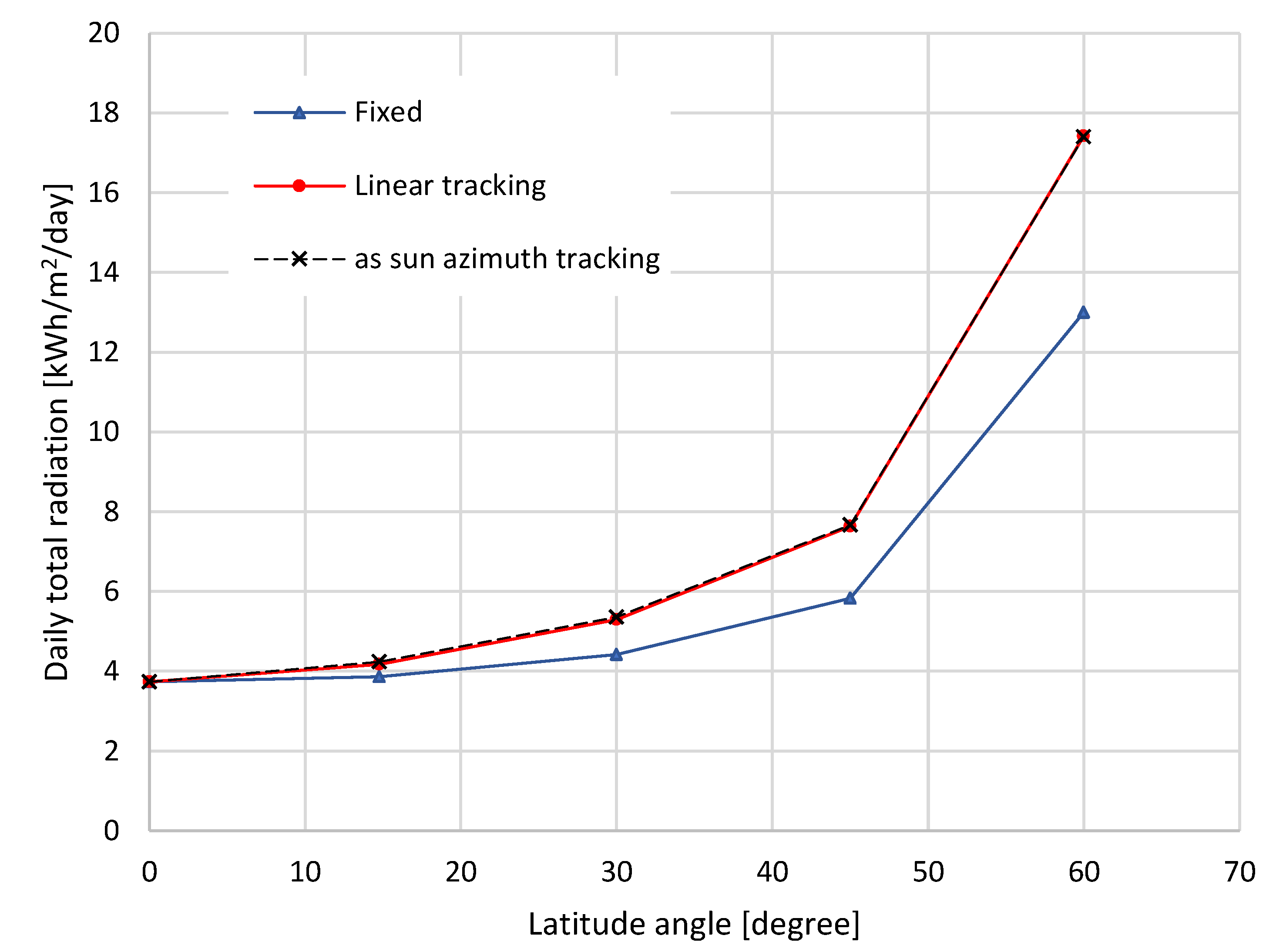

Table 1.
Mean day of the month, recommended days for months and values of N by months.
| Months | n for ith Day of Month | Mean Day of Month | Day of Year | Declination |
|---|---|---|---|---|
| January | i | 17 | 17 | -20.9 |
| February | 31+i | 16 | 47 | -13 |
| March | 59+i | 16 | 75 | -2.4 |
| April | 90+i | 15 | 105 | 9.4 |
| May | 120+i | 15 | 135 | 18.8 |
| June | 151+i | 11 | 162 | 23.1 |
| July | 181+i | 17 | 198 | 21.2 |
| August | 212+i | 16 | 228 | 13.5 |
| September | 243+i | 15 | 258 | -2.2 |
| October | 273+i | 15 | 288 | -9.6 |
| November | 304+i | 14 | 318 | -18.9 |
| December | 334+i | 10 | 344 | -23 |
Disclaimer/Publisher’s Note: The statements, opinions and data contained in all publications are solely those of the individual author(s) and contributor(s) and not of MDPI and/or the editor(s). MDPI and/or the editor(s) disclaim responsibility for any injury to people or property resulting from any ideas, methods, instructions or products referred to in the content. |
© 2025 by the authors. Licensee MDPI, Basel, Switzerland. This article is an open access article distributed under the terms and conditions of the Creative Commons Attribution (CC BY) license (https://creativecommons.org/licenses/by/4.0/).
Copyright: This open access article is published under a Creative Commons CC BY 4.0 license, which permit the free download, distribution, and reuse, provided that the author and preprint are cited in any reuse.


