Submitted:
17 September 2025
Posted:
19 September 2025
You are already at the latest version
Abstract
The understanding of coastal ecosystems regarding variability and resilience under climatic and anthropogenic forcing is reliant upon long-term ecological records. We examined the Helgoland Roads time series (1968–2017), which includes temperature, salinity, nutrients (nitrate, phosphate), and biological parameters (diatoms and Acartia spp.). We applied autocorrelation, multi-taper spectral analysis, wavelet and cross-wavelet transforms to identify dominant temporal patterns and scale-dependent interactions. Sea surface temperature shows consistent long-term warming, and sub-decadal (2–3 year) and decadal (7–8 year) oscillations reflect coherent patterns with the North Atlantic Oscillation and Arctic Oscillation. Salinity varied in antiphase to Elbe River discharge at 6–7 year scales, reflecting control of seasonal, riverine freshwater and salinity scenarios. Nutrients, both as declining long-term trends (particularly phosphate), are associated with seasonal to multi-year variability linked to episodic discharge events. Biological parameters had strong annual periodicities reflective of bloom cycles, but also variability above the annual limit. Diatoms responded to climatic, nutrient, biological responses at the 3–5 year scale associated with this ecological context, particularly nitrate and phosphate; Acartia (spp) respond to temperature, salinity and resource availability (diatoms) reflecting climate-nutrient-trophic linkages. This study indicate that Helgoland Roads is represented as a multi-scale, non-stationary system, in which climate variability, riverine input and ecological linkages are cascaded down to physical and chemical processes that structure biological communities. Spectral methods reveal scale-dependent synchrony and highlight risks of trophic mismatch under climate change, emphasizing the importance of sustained, high-frequency monitoring.
Keywords:
Helgoland Roads
; spectral analysis
; wavelet transform
; nutrients diatoms
; climate variability
1. Introduction
Understanding both the spatial and temporal variability of physical, chemical, and biological condition of coastal seas is fundamental for predicting the response of the ecosystem to changes caused by climate forcing and human activity. The North Sea, being among the most studied shelf seas in the world, has also shown significant changes to its temperature, salinity, meaning of nutrients, and the communities of plankton in the past the decades [1,2,3]. The Helgoland Roads (HR) long-term ecological time series dataset began in 1962 and represents the longest continuous high frequency marine dataset in the world. It presents a unique opportunity for assessing multi-scale variability and driver-response relationships of a coastal ecosystem [4,5]
Prior studies have shown warming trends, noticeable shifts in nutrient availability, and changes in plankton phenology at HR [3,6]. Climate indices like North Atlantic Oscillation (NAO), and the Arctic Oscillation (AO), and also terrestrial freshwaters discharged from the Elbe river, have established their importance at the major drivers of hydrographic and ecological variability in the German Bight [7,8] but the temporal dynamics of these linkages are non-stationary and vary in strength and scale through time thus complicating the ability to isolate ecosystem response with static correlations.
Spectral methods represent strong methods for disentangling these interpretations by resolving dominant frequencies and time-localized interactions. The multi-taper method, wavelet transform, and cross-wavelet techniques can characterize linear and non-linear signals, allowing for temporal and spatial assessment of climate driver responses linked to biological responses [9,10].
The goal of this study is to assess the scope and nature of interannual to decadal variability in the physical (sea surface temperature, salinity, Secchi depth), chemical (nitrate, phosphate) and biological (diatoms, Acartia spp.) parameters at Helgoland Roads, and to understand how climate oscillations and river discharges act as modifiers to these dynamics. We aspire to provide new knowledge and understanding of the multi-scale coupling of physical, chemical, and biological interactions in a coastal shelf sea system, through the application of spectral and wavelet methods to five decades of HR time series.
2. Methods
2.1. Data Sources
Our study employed work-daily Helgoland Roads time series datasets for physical variables (Sea Surface Temperature [°C], Salinity, Secchi Depth [m]), chemical variables (nitrate NO₃⁻ [µmol L⁻¹], phosphate PO₄³⁻ [µmol L⁻¹]), and biological variables (total diatom abundance [cells L⁻¹], Acartia spp. abundance [ind. m⁻³]). These datasets were collected (and licensed) from the long-term ecological data set from the Alfred Wegener Institute (AWI) long-term ecological research program [11].
To represent terrestrial forcing, monthly Elbe River discharge data were sourced from the Global Runoff Data Centre [12]. Large-scale atmospheric forcing was characterized by monthly North Atlantic Oscillation (NAO) [13] and Arctic Oscillation (AO) [14] indices obtained from the U.S. National Weather Service Climate Prediction Center.
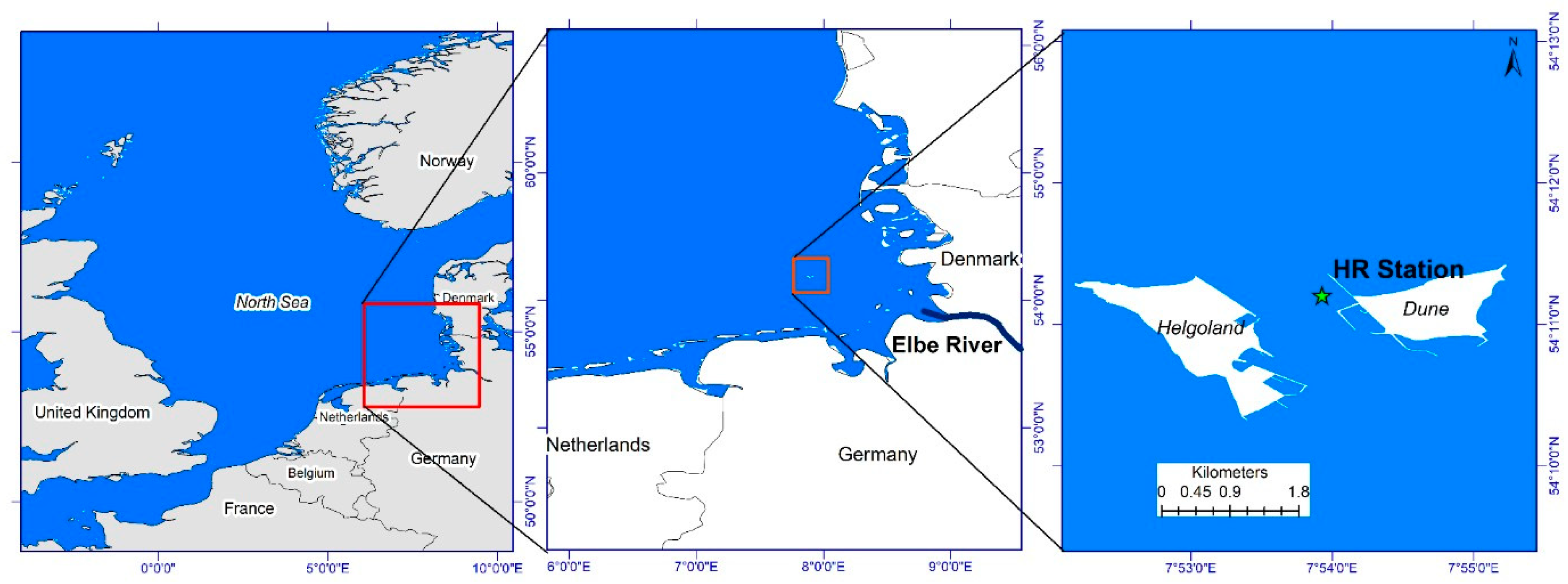
The Helgoland Roads (HR) time series station is situated in the German Bight of the southeastern North Sea (54°11′ N, 7°54′ E), in a tidal channel between the main island of Helgoland and the small island of Düne. The site is located about 60 km offshore from the German mainland, and is subjected to the impacts of open North Sea conditions (westward) as well as some terrestrial inputs predominantly from the Elbe River [15]. The German Bight is a shallow shelf-sea environment (normal depth 10–40 m) with semidiurnal tides and an average range of ~2.3m. Seasonal variability of temperature, salinity and nutrient concentrations can be substantial in this area [16].
Figure 1.
Geographical location of the study area (data used from www.marineregions.org). Left panel shows the map of North Sea with a rectangular box indicating the location of the German Bight. Middle panel map shows a close up of the German Bight with a rectangular box showing the position of Helgoland. Right panel map shows the location of Helgoland Roads Times Series Station located between two islands i.e. Helgoland and Düne.
2.2. Preprocessing
All time series were averaged to monthly values to allow comparability across the physical, chemical, and biological variables. Anomalies were adjusted by normalizing them and seasonal cycles were removed by calculating the monthly climatological means (1968-2017), and these means were subtracted from the time series. This focused attention on interannual to decadal variability, and it normalized the annual cycle’s influence over the subsequent analyses.
The justification is clearly outlined in Figure 2. The left panel has the wavelet power spectrum of Temperature, based on original time series data, whereas the right panel is based on normalized anomalies of time series data of Temperature. In the case of original time series data, the power spectrum demonstrates only 1-year periodicity. There were no observable signals of inter-annual and inter-decadal variability in the power spectrum of Temperature data based on original time series, while very clearly displayed the existence of inter-annual and inter-decadal signals in the power spectrum of Temperature based on normalized anomalies.
2.3. Autocorrelation
The temporal persistence of each normalized anomaly series was examined using autocorrelation functions (ACF), computed for successive 10-year blocks and the entire study period. Statistical significance was determined using the Bartlett method for significance limits (±2 standard errors, p < 0.05). This step was used to detect the memory effects within the time series, and also lagged dependencies.
2.4. Multi-Taper Spectral Analysis
In order to identify the most important frequencies in each variable, we applied the multi-taper method (MTM) of spectral analysis. The MTM has better spectral stability and lower variance than classical Fourier transforms [17]. Peaks in the spectra that exceed the 95% confidence interval against a red-noise background, were regarded as significant. The MTM spectra were used to delineate stationary periodicities across physical, chemical, and biological parameters.
2.5. Wavelet Analysis
To capture the non-stationary nature of the time series, we used the continuous wavelet transform (CWT), employing the Morlet wavelet [9]. This allows us to both resolve the dominant modes of variability, as well as their temporal location. The statistical significance for the CWT were determined using a red-noise background spectrum, and we used the cone of influence (COI) to denote areas with potential edge effects.
2.6. Cross-Wavelet Analysis
Finally, for our scale dependant assessments of relationships between variables, we used the cross-wavelet transform (XWT) [10,18], which quantifies the shared power between pairs of time series and provides a measure of their relative phase (i.e., whether they vary in phase, anti-phase, or with time lags). In one case we analysed XWT patterns (i) between physical drivers and climate indices, (ii) salinity with Elbe discharge, (iii) nutrients with physical drivers, and (iv) biological parameters with aspects of their potential drivers. The arrows in the cross- wavelet spectra signal their relative phase relationship (i.e., arrows to the right related to in-phase, left related to anti-phase, while up and down arrow indicate leading and lagging likelihood respectively).
PAST 3X (version 3.20) tool was used for MTM analysis of the time series variables base on normalized anomalies and other statistical analyses including wavelet transform and cross-wavelet-transform [19] were completed in R Studio.
3. Results
3.1. Temporal Variability
Physical, chemical, and biological normalized monthly anomalies (Figure 3) show both long-term patterns and short-term variations after the seasonal cycle was removed. Sea surface temperature (SST) indicates a continuous upward trend since approximately the mid-1980s, reflecting a persistent background warming in the German Bight. Regional warming has occurring within interannual fluctuations, such as distinct warm anomalies (with reference to the mean climatological temperature in the region) observed during the early 1990s and again in the early 2000s. Likewise, salinity exhibits pronounced decadal variability, including freshening periods associated with enhanced riverine influence followed by recovery periods.
Nutrient concentrations are struggling to exhibit with similar long-term trajectories. Nitrate anomalies show a progressive downward trajectory throughout the 1980s and after, representing reductions in anthropogenic loading and nutrient management in the Elbe catchment. Phosphate displays downward anomalies with episodic fluctuations, particularly during the 1970s and early 2000s.
Biological variables have greatly differing temporal heterogeneity. Although diatom abundances do show episodic peaks, they are not in regular succession indicating bloom events and more long-term variability. The episodic peaks are most pronounced during the late 1980s and mid-2010s, Acartia spp. also demonstrated marked fluctuations; the abundances were also notably high during the mid-1980s and late 1990s, and in early 2010s demonstrating population dynamics operate at times scales of seasonal and multi-year time scales.
The autocorrelation analysis of the anomalies for consecutive decades (Figure 4) shows differences in persistence across variables. SST and salinity anomalies retain significant autocorrelation over multiple lags for all time blocks, indicating physical forcing has very long memory. By contrast, nitrate and phosphate anomalies displayed weaker autocorrelations with significance only observed for the shortest lags which is indicative of rapid turnover and sensitivity to incoming resources. The biological time series stress quite short persistence: total diatom and Acartia spp. anomalies were significantly autocorrelated only for lags of one year consistent with annual bloom and lifecycle of Acartia. Beyond this autocorrelation dissipated rapidly which illustrated dominance of short-term environmental variance over long-term memory.
3.2. Spectral Characteristics
The multitaper spectral analysis (Figure 5) identified dominant frequencies through the entire period of 1968–2017. SST and salinity exhibited strong periodicities centered at 7-8 years and significant sub-decadal oscillations between 2-3 years. These periodicities relate directly to known modes of North Atlantic climate variability including the North Atlantic Oscillation and Atlantic Multidecadal Oscillation. In contrast to the physical variables, the nutrient time series were irregularly peaked but included both high frequencies (0.5–1 year) and longer cycles (3–7 years), indicating both seasonal forcing and hydroclimatic variability with predicted changes in nutrient concentrations across regimes.
The dominant diatom abundance annual cycle is predictable with the appearance of spring blooms; however, the quantity of diatom abundance diverges by repeated peaks of episodic events, sustained up to 3-5 years, attributed to changes in nutrients or hydrographic changes. Acartia spp. also strongly represent an annual component but their spectra brings to light inter annual modes at 2-3 years, and decadal variability at 8 years. Both taxa strongly depict shifts in population dictated by shifts in environmental regime.
The wavelet power spectra (Figure 7) shows all periodicity as non-stationary in time. SST and salinity show strong 7-8 year cycles from 1980-1990, and subsequent 2.5-year oscillation from 1993 -1995. Nitrate and phosphate had both intermittently strong high frequency variability throughout 1970-2000, and phosphate had an additional strong 3-year mode between 2006-2011. Biological variables had a strongly consistent annual periodicity, while the remaining shifting multi- year variability show a variety of periodicities. For instance, within the time window of 2014-2016, the diatom abundance periodically demonstrated a 3-year periodicity and was demonstrably periodic at 5 years from 1988-1992. The Acartia spp. had strong annual datasets during the 1980’s, while also reflecting multi-year variability, including perhaps, a strikingly prominent 15-year mode from 1990 to 2000. This indicates both physical and biological variability at Helgoland Roads will show distinct temporal windows of dominant periodicity, which will shift over time.
Figure 6.
Wavelet power spectrum analysis of normalized anomalies of the studied variables based on monthly mean with cone of influence (lighter shade smooth curve) and black lines indicate significant power on 95% level compared to red noise.
Figure 6.
Wavelet power spectrum analysis of normalized anomalies of the studied variables based on monthly mean with cone of influence (lighter shade smooth curve) and black lines indicate significant power on 95% level compared to red noise.
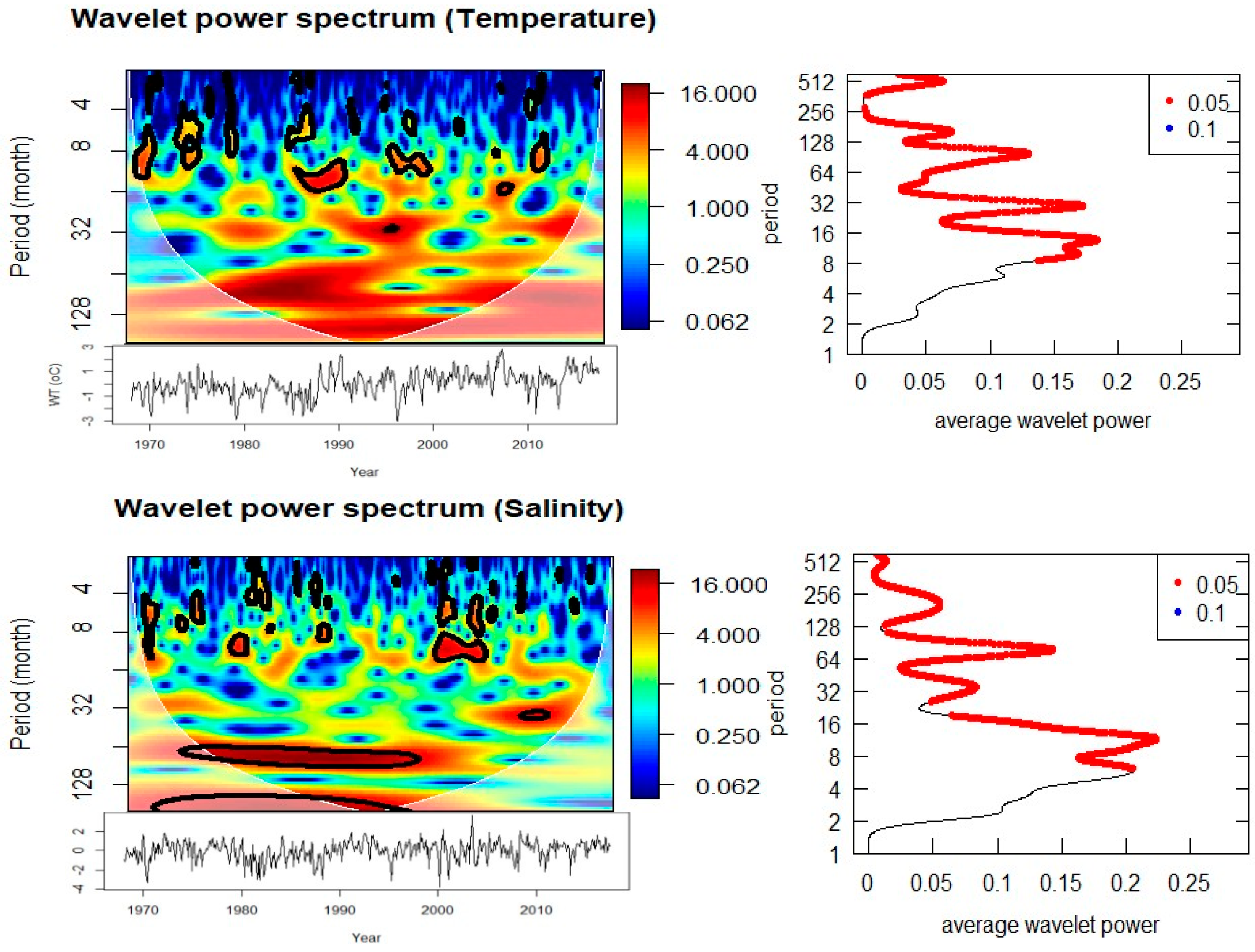
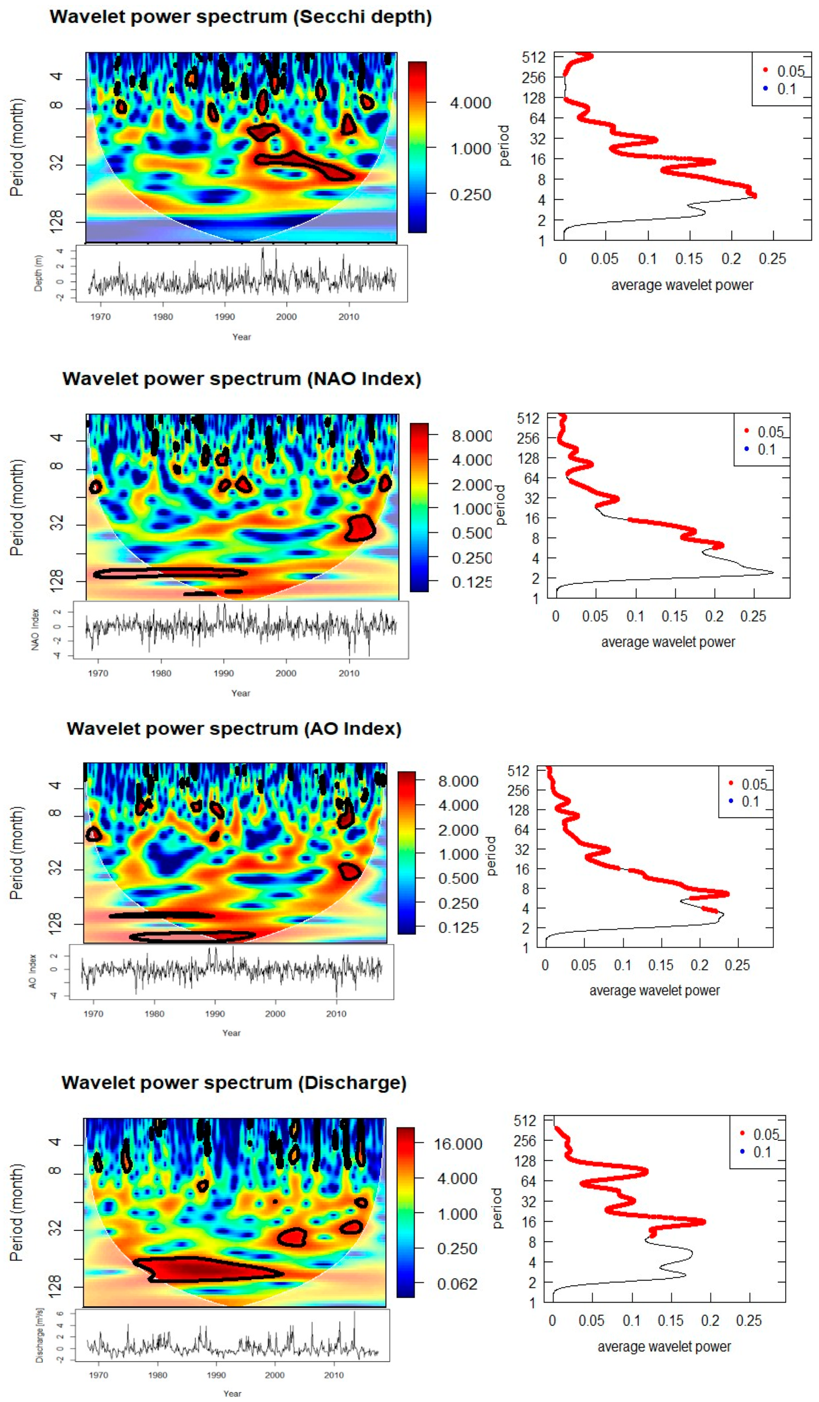
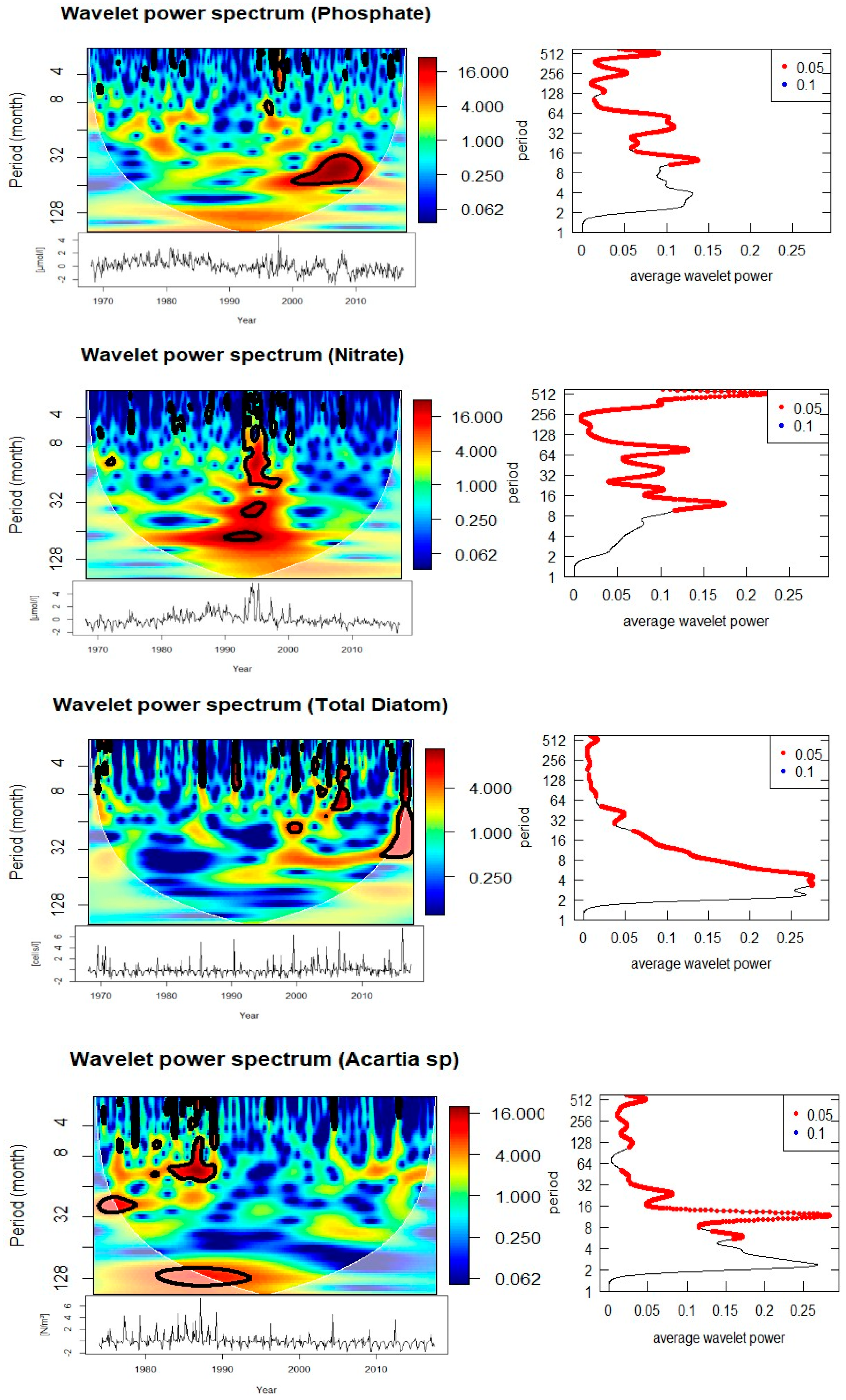
Figure 7.
Cross wavelet transform of the normalized anomaly of the time series of physical parameters with cone of influence (lighter shade smooth curve) and black lines indicate significant power on 95% level compared to red noise The relative phase relat ionship is shown as arrows (with in-phase pointing right, anti-phase pointing left). If the primary variable has positive normalized anomaly, the arrow direction is in-phase and vice versa.
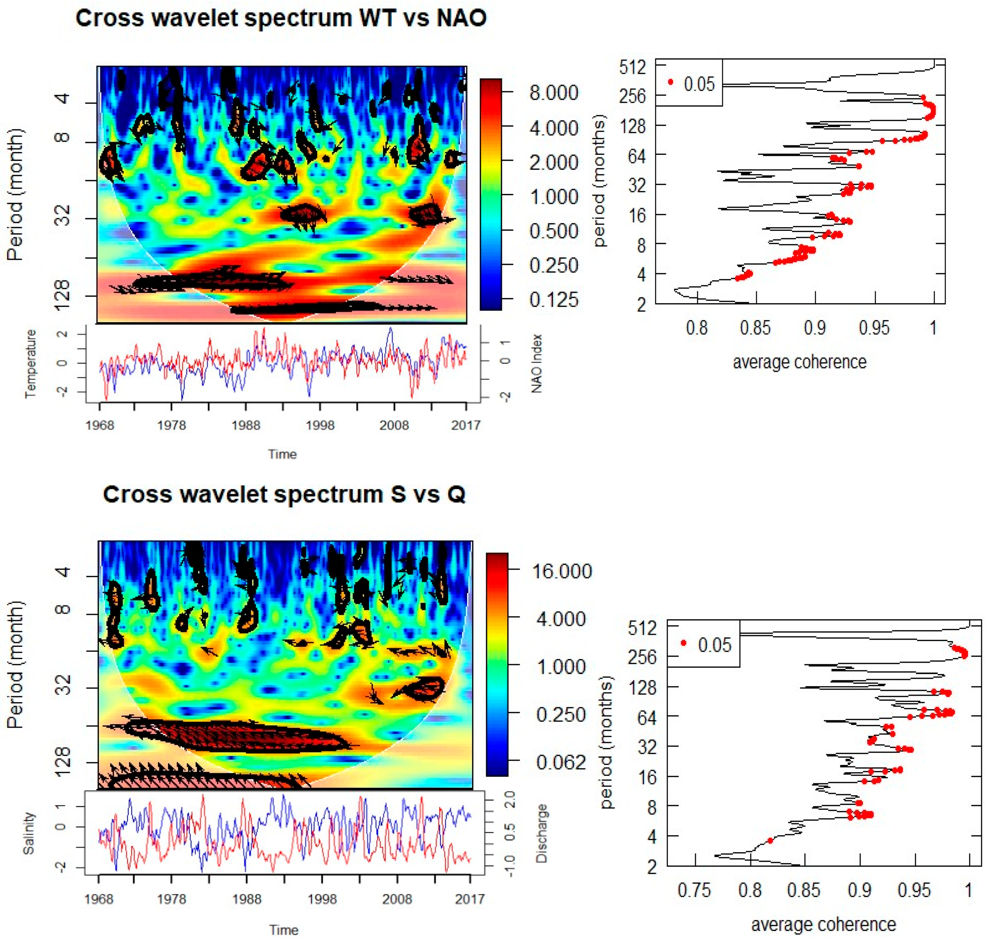
3.3. Links Between Physical Parameters and Large-Scale Drivers
Cross-wavelet analysis provides evidence for strong relationships between local physical parameters and large-scale climatic and terrestrial drivers (Figure 7, Table 1). SST is significantly coherent with both the North Atlantic Oscillation (NAO) and the Arctic Oscillation (AO) at periodicities of 2.5 years (1993–1995) and 7–8 years (1980–1990). Phase relationships indicate that these oscillations are in-phase, suggesting a direct and immediate response of SST to atmospheric forcing.
Salinity anomalies are strongly linked to Elbe River discharge, showing significant anti-phase relationships (180°) at 6–7 year cycles between 1970–2000. This reflects the dilution of seawater salinity by freshwater input during high discharge periods. Salinity also exhibits significant coherence with temperature at 7 years during 1980–1990 and with nitrate at both high-frequency (0.5–1 year, intermittent during 1970–2000) and multi-year (7 years, 1980–1998) scales. Phosphate also shows a 3-year anti-phase coherence with salinity between 2006–2011, suggesting that riverine and hydrographic processes strongly shape nutrient dynamics.
3.4. Biological Responses to Environmental Drivers
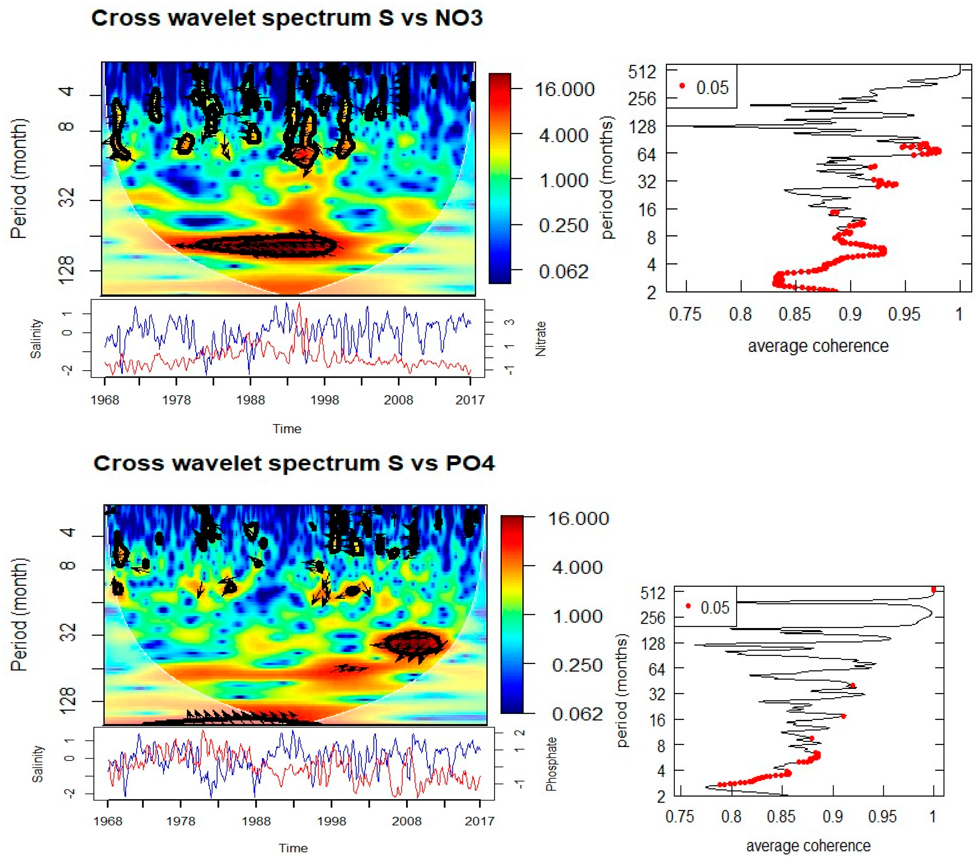
Cross-wavelet analyses of biological and environmental parameters (Figure 8, Table 1) reveal significant multi-scale coupling. Diatom abundance shows strong coherence with SST at both annual (0.5–1 year) and multi-year (3–5 year) scales. The phase relationships suggest that diatom peaks follow temperature anomalies with a lag, indicating modulation of bloom intensity and timing by thermal conditions. Significant coherence with salinity is observed at annual (0.5–1 year) and 5-year periods, with phase shifts indicating that diatom blooms are influenced by hydrographic variability. Associations with nitrate and phosphate occur at 3–5 year cycles, particularly during 1990–1995 (nitrate) and 2003–2010 (phosphate), suggesting a strong dependence of bloom dynamics on nutrient supply.
Acartia spp. show a similarly complex response. Significant coherence with SST is observed at annual (0.5–1 year, 1984–1988) and decadal (~8 years, 1985–1990) scales, with phase relationships indicating alternating in-phase and anti-phase dynamics. Salinity is coherent with Acartia spp. abundance at annual scales (1978–1988, intermittent) and at an 8-year cycle during 1988–1993. Nutrient relationships are evident at both annual (nitrate and phosphate during the 1980s) and longer (8-year nitrate, 15-year phosphate) scales. Importantly, Acartia spp. abundance also shows coherence with diatom abundance at both annual (1986–1987, 2007, 2016) and 3-year (2003–2010) scales, confirming trophic coupling between primary producers and zooplankton consumers.
4. Discussion
4.1. Variability
The robust 2–3 yr and 7–8 yr bands in SST and the significant cross-wavelet coherence with NAO/AO suggest a modulation of the thermal regimes at Helgoland Roads by large-scale atmospheric modes on sub-decadal cycles, superposed on the secular warming trend seen since at least the 1980s; consistent with more recent syntheses indicating ongoing warming in the German Bight and the North Sea [4,8]. The 2–3 yr and 7–8 yr bands persisted in our data record during 1980–1990 and 1993–1995 corresponding to periods with strong NAO/AO expression in the region [7,20]. Such a modulation of sub-decadal SST should be seen as one of the prime preconditions for the changes in phenology and trophodynamics seen across the North Sea planktonic community observed [21].
Cross-wavelet evidence demonstrating anti-phase salinity–discharge at ~6–7 years shows the overriding importance of riverine forcing at Helgoland Roads. Recent reviews have reaffirmed a river-dominated nutrient budget in the German Bight and south North Sea, with deposition from the atmosphere and inflow from the Atlantic being relatively minor and strongly seasonally driven [1,22]. The bigger picture is that river loads peaked in the 1980s and have declined (more rapidly for P than N) since, increasing the N:P ratio [1].
4.2. Ecological Response
The diatoms in Helgoland Roads demonstrate strong repeated annual (spring bloom) and secondary 3–5 yr bands that go weak and strong through time in each of your wavelets. The recent work shows that the spring bloom timing of diatoms is very resilient, while the magnitude and composition is variable interannually [6], and studies of “rapid succession” also suggest that even small physical–chemical windows can cause microplankton communities to be restructured in spring [23]. This fits well with your identification of coherence between diatoms and nitrate/phosphate at multi-year scales as it relates to nutrient supply that is driven by hydrographic and climate variability. Furthermore, taxonomic and metabarcoding studies have shown that phases of diversification and turnover of diatom and dinoflagellate assemblages are still happening in Helgoland [3,5], suggesting that physical–chemical envelopes we have found in the spectral analysis may be expressed as community composition changes even while bulk bloom timing is consistent.
Cross wavelet suggests that Acartia spp. responded at annual, interannual (2–3 yr), and longer (~8–15 yr) scales, there is also significant coupling to SST, salinity, and nutrients—and to diatoms at annual, and 3-yr bands. This fits well with the multi-decadal copepod studies documenting trends in copepod phenology and biomass across the North Sea; at Helgoland, studies that span decades note that temperature acts as a key variable regulating copepod reproduction and phenology [3,21]. The coherence with diatoms at both short and interannual time scales may indicate alternating bottom-up trophic control (due to prey availability) and lags (from hydroclimate-mediated changes in food quality) that align with recent reports of reorganization in copepod communities with warming [2].
When taken together, the spatially introduced NAO/AO-driven temperature field (T), riverine-controlled salinity/nutrient loading (S), and biological periodicity (e.g., total diatoms and Acartia spp.), provide a picture of a non-stationary multi-scale coupled system in a highly dynamic, coastal ecosystem. With river discharge at high levels (or years of high magnitude) and with a positive NAO, we generally expect a fresher, more stratified, and nutrient-rich condition in spring to promote diatom blooms and create stronger annual-band connections with Acartia. Though, in periods dominated by lower discharge regimes and altered N:P stoichiometry, these blooms may be nutrient limited, and be compositional, while grazer/consumer responses appear more of a lagged/interannual nature, strengthening the 3–5 yr coherence bands observed here. Furthermore, regional syntheses show similar relationships to those discussed here, decreasing nutrient concentrations, mixed effects of temperature on Chl-a, and spatial differences in plankton response to hydrodynamic context [4,8].
4.3. Implications and Outlook
From a methodology perspective, the use of multi-taper spectral analysis and (cross-) wavelet analysis together creates a meaningful framework to identify the temporal scales and windows of opportunity where environmental drivers and biological responses covary, something conventional time-series analysis approaches are unable to isolate in a single timeframe. From an ecological perspective, we have used the annual and interannual bands to identify both risks of short-term match–mismatch, as well as multi-year changes in the community that are relevant to trophic transfer in the German Bight. Incorporating Helgoland Roads monitoring with trait-based analysis of zooplankton [2] and molecular community analysis [5] will be critical for translating these spectral trends into mechanistic information of food-web dynamics under climate change.
5. Conclusions
A temporal analysis using spectral and wavelet analysis of nearly a half-century of time series data from Helgoland Roads identified scale-dependent variability of environmental drivers (i.e., physical, chemical, biological) in the German Bight. There was a significant warming trend in sea-surface temperature, which was linked to sub-decadal to decade-long oscillations that were correlated with larger climate variability (for example, the NAO and AO). Salinity was found to be temporally and spatially characterized by Elbe River discharge, demonstrating the influence of riverine influences forced on coastal hydrodynamics. Nutrients decreased with human management, but also displayed periodic, multi-year dynamics; however, diatoms and Acartia spp. had distinct annual patterns, with inter-annual and decadal variability.
Further, the coherence identified with the cross-wavelet analysis demonstrated that climate forcing, riverine inputs, and nutrient dynamics interacted with each other, as well as the biological communities at various temporal scales. Ultimately, the findings revealed that the system operates as a non-stationary tightly coupled system from an ecological system perspective where environmental controls cascade down physical, chemical drivers into ecosystem dynamics. Critically, the recognition that scales of climate forcing and biological responses were both stable and shifting scales means that ecosystem processes that are connected through trophic interactions may be exposed to mismatching events from climate change.
In the last instance, acknowledging dominant time scales of variability emphasizes the importance of sustained long-term, high frequency monitoring of coastal seas. The ongoing measurements at Helgoland Roads provide relevant information for ecosystem resilience, enable foreseeing regime shifts, and promote adaptive management of the North Sea.
Data Availability Statement
The original contributions presented in this study are included in the article. Further inquiries can be directed to the corresponding author.
Acknowledgments
This paper and related research have been conducted during and with the support NF-POGO Centre of Excellence, Alfred Wegener Institute (AWI), Germany (https://pogo-ocean.org/capacity-development/centre-of-excellence/). Author would like to thank Helgoland Roads time series by AWI, located at the island of Helgoland in the German Bight. This research was guided by Dr. Mirco Scharfe, Environmental Scientist, AWI, who passed away on 11th August 2019.
Conflicts of Interest
The authors declare no conflicts of interest.
References
- J. E. E. van Beusekom et al., “Wadden Sea Eutrophication: Long-Term Trends and Regional Differences,” Front Mar Sci, vol. 6, Jul. 2019. [CrossRef]
- M. M. Deschamps, M. Boersma, and L. Giménez, “Responses of the mesozooplankton community to marine heatwaves: Challenges and solutions based on a long-term time series,” Journal of Animal Ecology, vol. 93, no. 10, pp. 1524–1540, Oct. 2024. [CrossRef]
- K. H. Wiltshire et al., “Resilience of North Sea phytoplankton spring bloom dynamics: An analysis of long-term data at Helgoland Roads,” Limnol Oceanogr, vol. 53, no. 4, pp. 1294–1302, Jul. 2008. [CrossRef]
- K. Kordubel et al., “Long-term changes in spatiotemporal distribution of Noctiluca scintillans in the southern North Sea,” Harmful Algae, vol. 138, p. 102699, Sep. 2024. [CrossRef]
- L. Käse et al., “Metabarcoding analysis suggests that flexible food web interactions in the eukaryotic plankton community are more common than specific predator–prey relationships at Helgoland Roads, North Sea,” ICES Journal of Marine Science, vol. 78, no. 9, pp. 3372–3386, Nov. 2021. [CrossRef]
- M. Scharfe and K. H. Wiltshire, “Modeling of intra-annual abundance distributions: Constancy and variation in the phenology of marine phytoplankton species over five decades at Helgoland Roads (North Sea),” Ecol Modell, vol. 404, pp. 46–60, Jul. 2019. [CrossRef]
- U. Callies and M. Scharfe, “Mean spring conditions at Helgoland Roads, North Sea: Graphical modeling of the influence of hydro-climatic forcing and Elbe River discharge,” J Sea Res, vol. 101, pp. 1–11, Jul. 2015. [CrossRef]
- F. de L. L. de Amorim, A. Balkoni, V. Sidorenko, and K. H. Wiltshire, “Analyses of sea surface chlorophyll a trends and variability from 1998 to 2020 in the German Bight (North Sea),” Ocean Science, vol. 20, no. 5, pp. 1247–1265, Oct. 2024. [CrossRef]
- C. Torrence and G. P. Compo, “A Practical Guide to Wavelet Analysis,” Bull Am Meteorol Soc, vol. 79, no. 1, pp. 61–78, Jan. 1998. [CrossRef]
- A. Grinsted, J. C. Moore, and S. Jevrejeva, “Application of the cross wavelet transform and wavelet coherence to geophysical time series,” Nonlinear Process Geophys, vol. 11, no. 5/6, pp. 561–566, Nov. 2004. [CrossRef]
- K. H. Wiltshire et al., “Helgoland Roads, North Sea: 45 Years of Change,” Estuaries and Coasts, vol. 33, no. 2, pp. 295–310, Mar. 2010. [CrossRef]
- GRDC, “Elbe River discharge data. GRDC Monthly Discharge Dataset (station-level daily/monthly discharge).”.
- NCEI, “North Atlantic Oscillation (NAO) Index. National Oceanic and Atmospheric Administration. NOAA National Centers for Environmental Information.”.
- NCEI, “Arctic Oscillation (AO) Index. National Oceanic and Atmospheric Administration. NOAA National Centers for Environmental Information.”.
- T. Raabe and K. H. Wiltshire, “Quality control and analyses of the long-term nutrient data from Helgoland Roads, North Sea,” J Sea Res, vol. 61, no. 1–2, pp. 3–16, Jan. 2009. [CrossRef]
- K.-C. Emeis et al., “The North Sea — A shelf sea in the Anthropocene,” Journal of Marine Systems, vol. 141, pp. 18–33, Jan. 2015. [CrossRef]
- D. J. Thomson, “Spectrum estimation and harmonic analysis,” Proceedings of the IEEE, vol. 70, no. 9, pp. 1055–1096, 1982. [CrossRef]
- L. Wang et al., “Nutrients and Environmental Factors Cross Wavelet Analysis of River Yi in East China: A Multi-Scale Approach,” Int J Environ Res Public Health, vol. 20, no. 1, p. 496, Dec. 2022. [CrossRef]
- A. Rösch and H. Schmidbauer, “WaveletComp 1.1: A guided tour through the R package,” URL: http://www. hsstat. com/projects/WaveletComp/WaveletComp_guided_tour. pdf, 2016.
- G. Beaugrand, P. C. Reid, F. Ibañez, J. A. Lindley, and M. Edwards, “Reorganization of North Atlantic Marine Copepod Biodiversity and Climate,” Science (1979), vol. 296, no. 5573, pp. 1692–1694, May 2002. [CrossRef]
- M. M. Deschamps, M. Boersma, C. L. Meunier, I. V Kirstein, K. H. Wiltshire, and J. Di Pane, “Major shift in the copepod functional community of the southern North Sea and potential environmental drivers,” ICES Journal of Marine Science, vol. 81, no. 3, pp. 540–552, Apr. 2024. [CrossRef]
- A. Siems, T. Zimmermann, T. Sanders, and D. Pröfrock, “Dissolved trace elements and nutrients in the North Sea—a current baseline,” Environ Monit Assess, vol. 196, no. 6, p. 539, Jun. 2024. [CrossRef]
- L. Käse et al., “Rapid succession drives spring community dynamics of small protists at Helgoland Roads, North Sea,” J Plankton Res, vol. 42, no. 3, pp. 305–319, May 2020. [CrossRef]
Figure 2.
Wavelet power spectrum of Temperature: for original time series data (left) and for normalized anomalies (right).
Figure 2.
Wavelet power spectrum of Temperature: for original time series data (left) and for normalized anomalies (right).
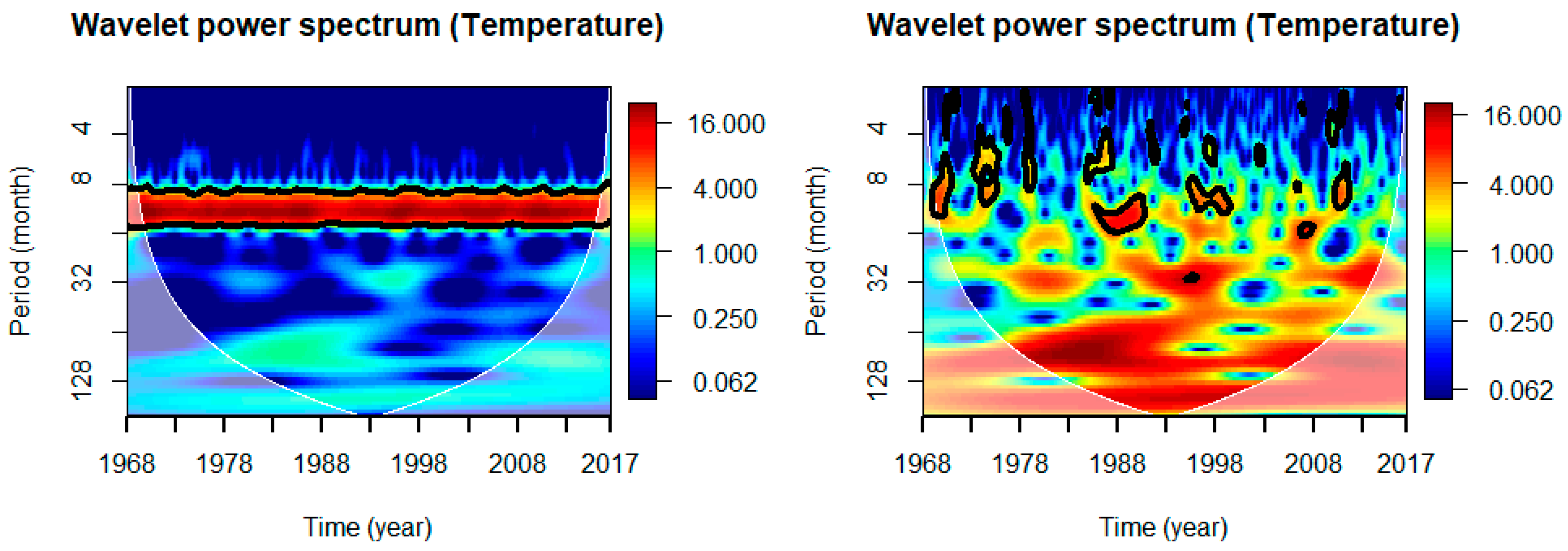
Figure 3.
Normalized anomalies of the monthly time series of the variables (without seasonality).
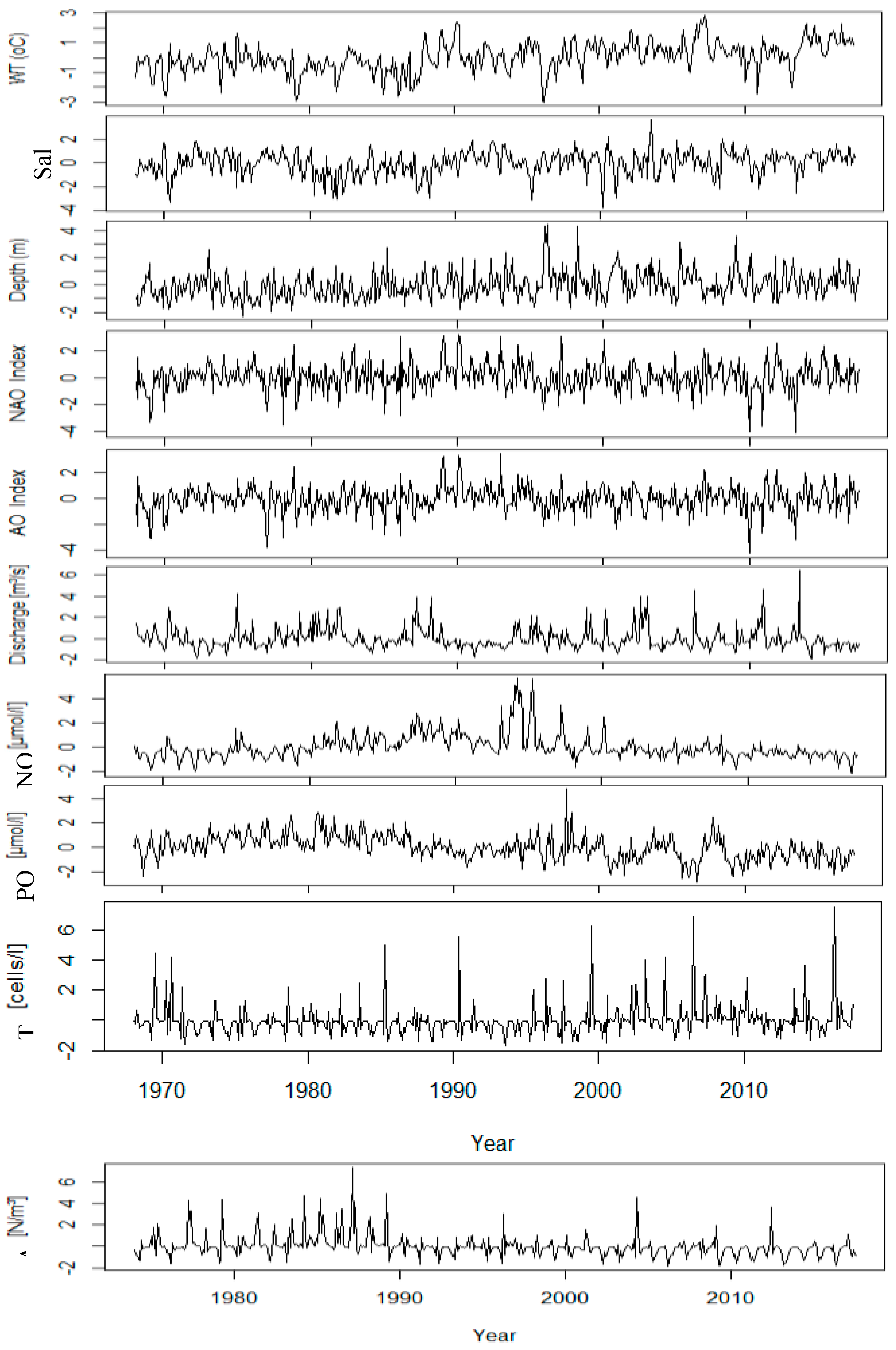
Figure 4.
Autocorrelation of the time series anomalies for 10-year blocks from 1968-2017. The dashed lines represent the range outside which autocorrelation is statistically significant (P<0.05; ±2 standard errors). A: 1968-1977, B: 1978-1987, C: 1988-1997, D: 1998-2007, E: 2008-2017 and F: 1968-2017.
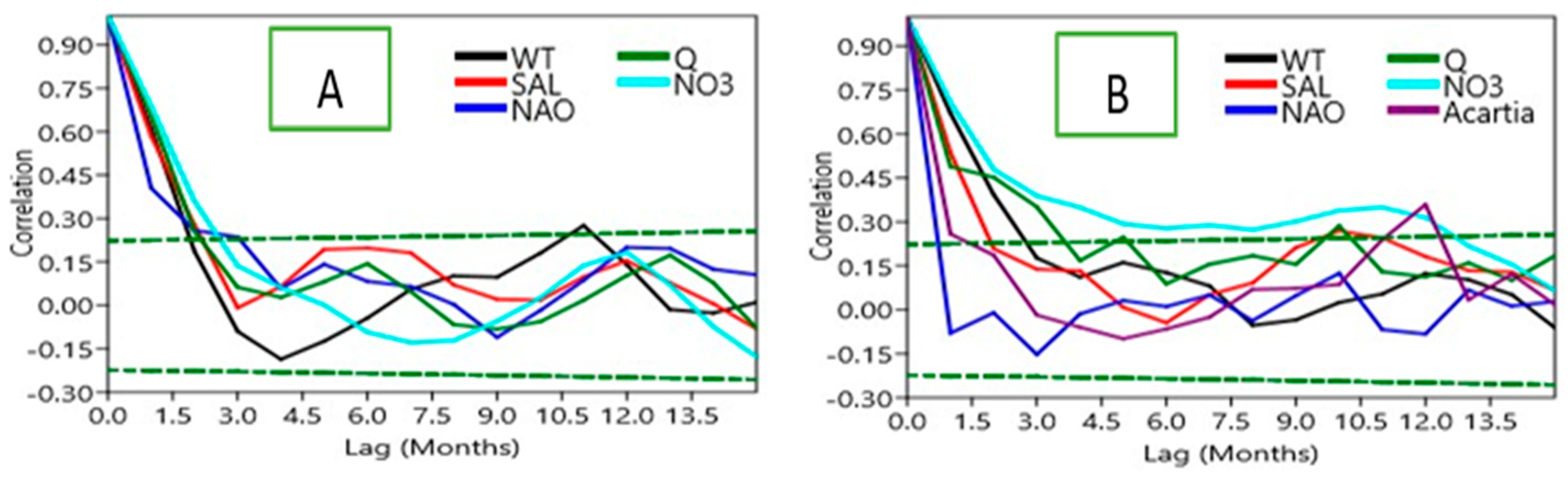
Figure 5.
Multitaper spectral analysis for the whole time series period.
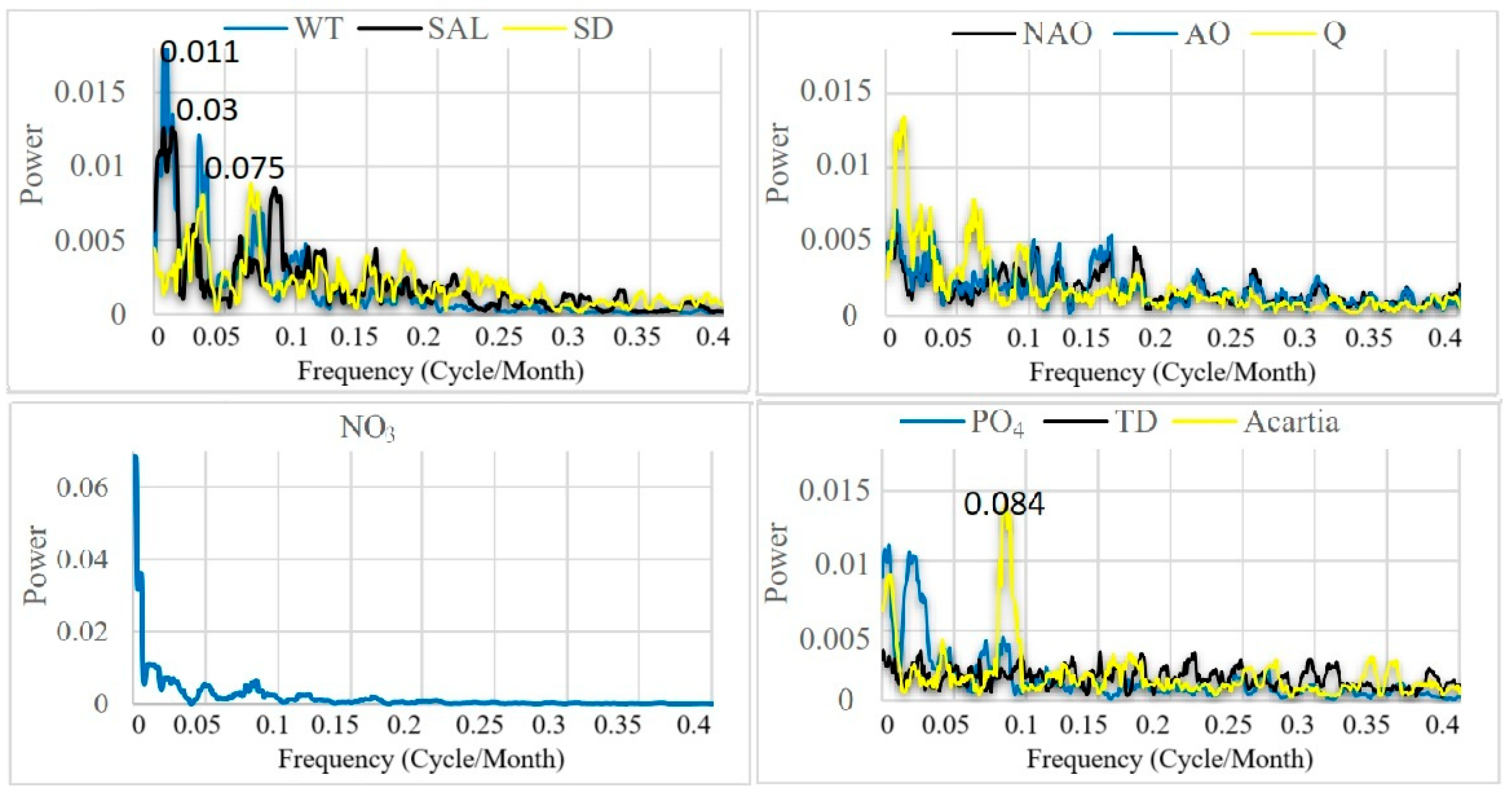
Figure 8.
Cross wavelet transform of the normalized anomaly of the time series with with cone of influence (lighter shade smooth curve) and black lines indicate significant power on 95% level compared to red noise The relative phase relationship is shown as arrows (with in-phase pointing right, anti-phase pointing left). If the primary variable has positive normalized anomaly, the arrow direction is in-phase and vice versa.
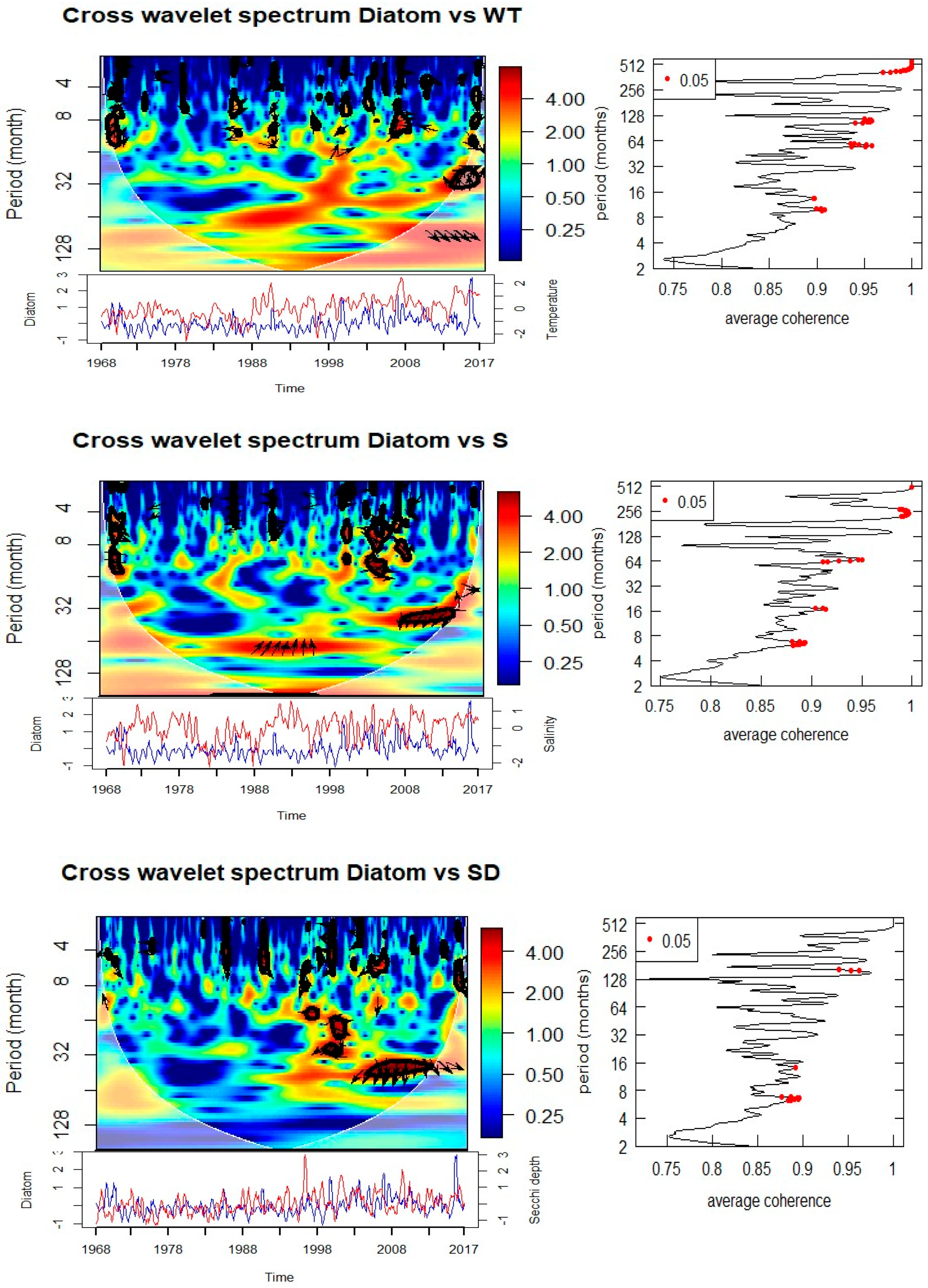
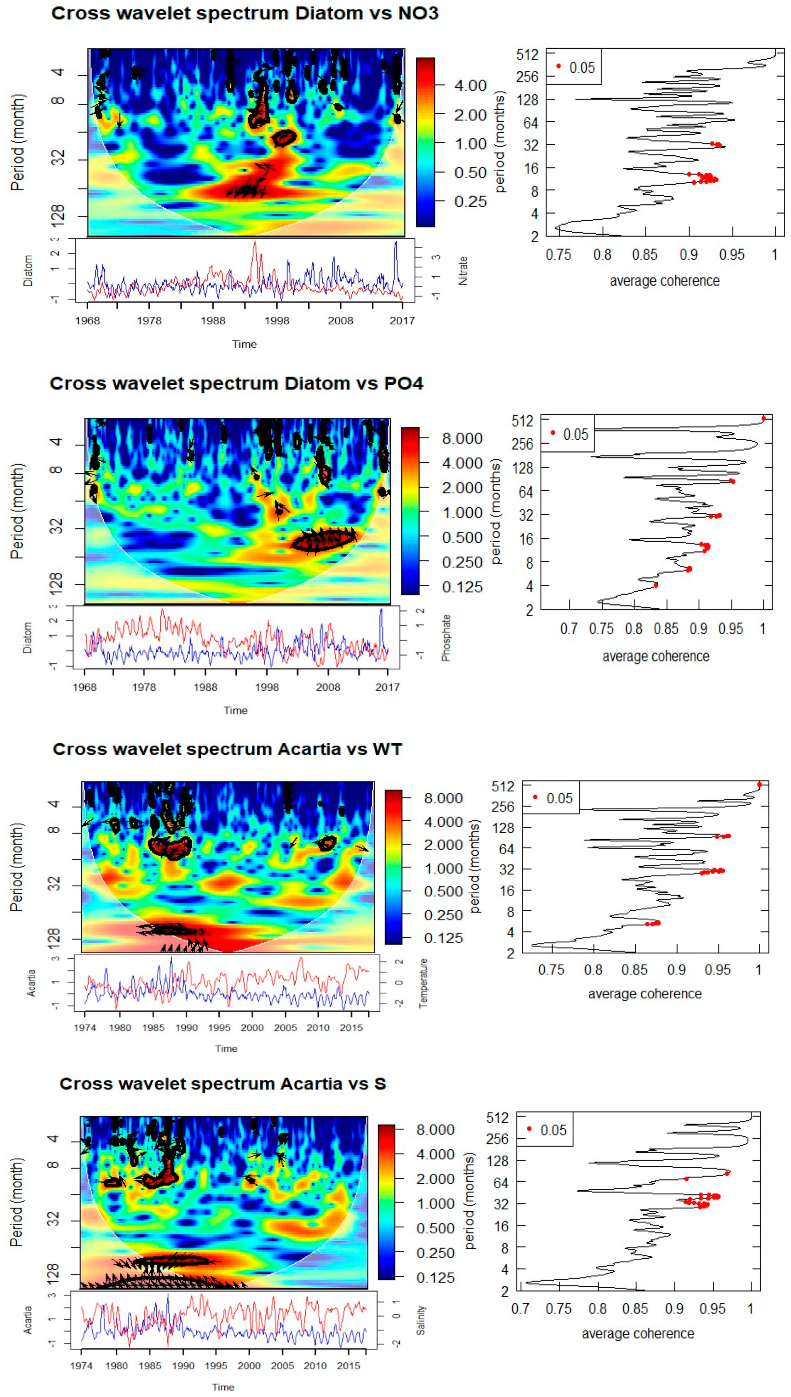

Table 1.
Summary of the drivers of T, S, and Q following cross wavelet spectrum. Observed periodicity and associated significant time period and phase angle are also listed.
Table 1.
Summary of the drivers of T, S, and Q following cross wavelet spectrum. Observed periodicity and associated significant time period and phase angle are also listed.
| Variables | Periodicity (Year) | Time periods | Phase angle |
| For Temperature | |||
| NAO | 2.5 | 1993-1995 | 90 |
| 07-Aug | 1980-1990 | 0 | |
| AO | 2.5 | 1993-1995 | 90 |
| 07-Aug | 1980-1990 | 0 | |
| For Salinity | |||
| Temperature | 7 | 1980-1990 | 90 |
| Discharge | 06-Jul | 1970-2000 | 180 |
| NO3 | 0.5-1 | 1970-2000 (intermittent) | 180 |
| 7 | 1980-1998 | 180 | |
| PO4 | 3 | 2006-2011 | 180 |
| For Total Diatom | |||
| Temperature | 0.5-1 | 1970 | 270 |
| 3 | 2014-2016 | 270 | |
| 5 | 1988-1992 | ||
| Salinity | 0.5-1 | 1970 , 2004 | 0 |
| 0.5-1 | 2008-2012 | 90 | |
| 5 | 1988-1995 | 270 | |
| NO3 | 03-May | 1990-1995 | 180 |
| PO4 | 3 | 2003-2010 | 180 |
| For Acartia spp. | |||
| Temperature | 0.5-1 | 1984-1988, | 180 |
| 8 | 1985-1990 | 180 | |
| Salinity | 1 | 1978-1988 (intermittent) | 180 |
| 8 | 1988-1993 | 90 | |
| NO3 | 1 | 1977-1988 (intermittent) | 0 |
| 8 | 1986-1996 | 0 | |
| PO4 | 1 | 1982-1987 | 270 |
| 2.5 | |||
| 15 | 1990-2000 | 0 | |
| Total Diatom | 1 | 1986-1987, 2007, 2016 | 180 |
| 3 | 2003-2010 | 180 | |
Disclaimer/Publisher’s Note: The statements, opinions and data contained in all publications are solely those of the individual author(s) and contributor(s) and not of MDPI and/or the editor(s). MDPI and/or the editor(s) disclaim responsibility for any injury to people or property resulting from any ideas, methods, instructions or products referred to in the content. |
© 2025 by the authors. Licensee MDPI, Basel, Switzerland. This article is an open access article distributed under the terms and conditions of the Creative Commons Attribution (CC BY) license (http://creativecommons.org/licenses/by/4.0/).
Copyright: This open access article is published under a Creative Commons CC BY 4.0 license, which permit the free download, distribution, and reuse, provided that the author and preprint are cited in any reuse.


