
Submitted:
18 September 2025
Posted:
18 September 2025
You are already at the latest version
Abstract
Virtual Power Plant (VPP) is capable of aggregating and intelligently coordinating diverse distributed energy resources, among which the accuracy of load forecasting is a key factor in ensuring their regulation capability. To address the periodicity and complex nonlinear fluctuations of electricity load data, this study introduces a Cyclic Order Mapping (COM) encoding method, which maps weekly and intraday sequences into continuous ordered variables on the unit circle, thereby effectively preserving load periodic features. On the basis of the COM encoding, a novel forecasting model is proposed by integrating Bidirectional Long Short-Term Memory (BiLSTM) networks, an efficient self-attention mechanism, and the Kolmogorov–Arnold Network (KAN). This model is termed BiLSTM-Att-KAN. Comparative and ablation experiments were conducted to assess the scientific validity and predictive accuracy of the proposed approach. The results confirm its superiority, achieving a Root Mean Square Error (RMSE) of 141.403, a Mean Absolute Error (MAE) of 106.687, and a coefficient of determination (R2) of 0.962. These findings demonstrate the effectiveness of the proposed model in enhancing load forecasting performance for VPP applications.
Keywords:
virtual power plants
; COM encoding
; electrical load forecasting
; BiLSTM-Att-KAN
1. Introduction
The efficient utilization of energy and the pursuit of sustainable development are fundamental objectives of the modern electrical industry. As a key technology driving digital transformation, the Virtual Power Plant (VPP) integrates distributed renewable energy sources, energy storage systems, and flexible loads. By intelligently optimizing dispatch strategies and market trading mechanisms, a VPP enhances grid flexibility, reduces carbon emissions, and facilitates the transition of electrical systems toward cleaner, low-carbon, and intelligent development [1,2,3,4]. Nevertheless, in the context of intelligent VPP operation, accurate electrical load forecasting is a critical prerequisite for ensuring efficient dispatch and effective market responsiveness [5]. Consequently, the development of high-precision load forecasting models constitutes a core technological foundation for enabling VPPs to flexibly aggregate distributed resources, support carbon reduction, and improve economic performance [6].
In VPP systems, electrical load fluctuations exhibit distinct periodic characteristics across both short and long term time scales. At the short-term level, with daily monitoring cycles, load curves demonstrate clear diurnal periodicity, characterized by pronounced day–night variations that closely correspond to human activity patterns [7]. At the long-term scale, seasonal temperature changes lead to a dual-peak pattern, driven by summer cooling demand and winter heating loads [8]. Beyond these periodic features, however, the randomness of human behavior and the nonlinear response to external disturbances introduce additional complexity to the load profile. As a result, effectively extracting and modeling the multi-scale, composite temporal patterns of load data while mitigating noise interference remains a key challenge for improving the accuracy of load forecasting in VPP applications.
Electrical load forecasting models can generally be classified into mechanistic models and data-driven models. Mechanistic approaches require substantial domain expertise and detailed system knowledge, which often limits their applicability. With the rapid advancement of artificial intelligence, machine learning and deep learning techniques have emerged as powerful alternatives for load forecasting. These data-driven approaches can automatically extract complex patterns from large-scale historical datasets, thereby improving the forecasting accuracy of fluctuating load series [9]. In general, data-driven models can be divided into static models, represented by machine learning methods [10], and dynamic models, represented by deep learning methods [11]. Commonly applied machine learning algorithms for load forecasting include BP neural networks (BPNN) [12], support vector regression (SVR) [13], and random forests (RF) [14], whose effectiveness has been widely demonstrated [15]. However, such models rely on a static modeling framework and often assume that data are independent and identically distributed. As a result, they fail to capture temporal dependencies and struggle to adapt to the time-varying characteristics of electrical load. In recent years, recurrent neural networks (RNNs) [16] have gained prominence due to their recurrent architecture, which allows them to retain historical information in temporal tasks and thereby overcome the limitations of static models. However, when dealing with long-term sequential tasks, increasing the depth of RNN layers leads to difficulties during backpropagation. Owing to the chain rule, this process is highly prone to exponential gradient explosion or vanishing, which in turn degrades predictive performance. To mitigate this issue, long short-term memory (LSTM) networks [17] and gated recurrent unit (GRU) [18,19] introduce gating mechanisms to dynamically filter and update historical load information in real time. Building on these developments, bidirectional models based on LSTM and GRU, such as bidirectional long short-term memory (BiLSTM) networks [20] and bidirectional gated recurrent unit (BiGRU) [21], have been extensively studied and validated for time-series load forecasting. Transformers leverage a self-attention mechanism to effectively decouple the multi-scale temporal characteristics of electrical load, while positional encoding preserves temporal consistency, thereby ensuring reliable forecasting performance [22,23]. Despite their notable improvements in forecasting accuracy, the interpretability of these models remains limited due to their complex and implicit feature extraction mechanisms. This limitation constrains their decision-making credibility in practical electrical load forecasting applications. Kolmogorov–Arnold Network (KAN) replaces the fixed nonlinear transformations of traditional multilayer perceptron (MLP) with learnable activation functions [24]. In electrical load forecasting, KAN enables adaptive extraction of multi-scale features, thereby significantly enhancing both the approximation capability and interpretability of complex nonlinear systems. With continued research, numerous hybrid forecasting models have been developed to overcome the limitations of single models by performing multi-level extraction of time-series features [25,26,27].
In summary, electrical load forecasting still faces the following challenges:(1) traditional time-series encoding methods, such as one-hot encoding, often generate high-dimensional sparse representations when the number of feature variables is large, thereby increasing the risk of overfitting and weakening generalization performance. (2) most existing models struggle to jointly capture short-term dependencies and long-term correlations, as they tend to emphasize either local features or global structures without achieving effective integration. (3) the nonlinear characteristics of electrical load are difficult to approximate accurately with conventional fully connected layers, which constrains both forecasting accuracy and model reliability.
The main contributions of this paper can be summarized as follows:
- (1)
- This paper proposes a cyclic order mapping (COM) encoding method, which explicitly preserves the gradual periodic variation patterns of electrical load by mapping weekly and intraday time sequences to continuous ordered vectors on the unit circle. Moreover, owing to its constant dimensionality, COM encoding substantially reduces feature space complexity and mitigates overfitting problems caused by high-dimensional sparsity.
- (2)
- This paper constructs a BiLSTM-Att-KAN ensemble model that integrates BiLSTM, an efficient self-attention mechanism, and KAN. Specifically, the primary BiLSTM captures short-term dependencies and local features from raw load data, while the self-attention mechanism extracts long-term dependencies and global structures. A secondary BiLSTM then fuses these multi-scale temporal features to further enhance dynamic representation. Finally, KAN maps the refined features into accurate forecasting results. The synergistic interaction of these components effectively resolves the difficulty of jointly modeling short- and long-term dependencies and significantly improves predictive performance.
- (3)
- This paper replaces conventional fully connected layers with KAN, which enhances the model’s nonlinear fitting capability and improves the reliability of forecasting results. By transforming complex temporal features into accurate forecasting results, KAN effectively overcomes the limitations of conventional architectures and ensures high-quality load forecasting.
2. Virtual Power Plant
A VPP represents an integrated system enabled by advanced information and communication technologies in fusion with intelligent control strategies. Its primary function is the centralized aggregation, coordinated optimization, and flexible regulation of diverse distributed energy resources (DERs) [28], the structure of a VPP is shown in Figure 1. These DERs mainly include distributed renewable energy sources, controllable loads on the demand side, and various energy storage systems. By integrating geographically dispersed, heterogeneous, and inherently fluctuating resources into a single virtual entity with enhanced predictability, dispatchability, and rapid responsiveness, a VPP enables the efficient aggregation and intelligent management of multiple distributed resources.
This virtualization and integration capability enables the VPP to proactively respond to real-time grid demands by providing critical ancillary services to the electrical system. Such services include peak shaving and valley filling, balancing intraday load fluctuations, supplying reserve capacity, and enhancing system resilience against unexpected events. Through these functions, the VPP plays a vital role in supporting the secure, stable, and economically efficient operation of the electrical grid.
In the daily management and refined dispatch practices of electrical systems, accurate load forecasting not only provides essential data support and a scientific basis for dispatching decisions but also constitutes a crucial prerequisite for achieving deep collaborative interaction and efficient matching optimization among four key parties: the generation side, the grid, the load side, and energy storage. The accuracy of load forecasting directly determines the capability of a VPP for optimal coordinated control of aggregated resources, serving as a key input factor for enhancing overall energy utilization efficiency and system operational flexibility.
3. Methodology
3.1. COM Encoding
This paper proposes an innovative encoding method called COM encoding for periodic feature sequences. The core design principle is to project discrete temporal variables onto continuous ordered variables on the unit circle, thereby explicitly preserving the periodic patterns inherent in electrical load data. By mapping discrete temporal points—such as weekly sequence numbers and intraday time indices—onto continuous variables on the unit circle, the method achieves seamless integration of periodic characteristics. In doing so, it effectively resolves the endpoint discontinuity problem inherent in conventional discrete encoding approaches, ensuring the complete representation of periodic features. Moreover, this encoding approach not only maintains the sequential relationships within the time series but also precisely expresses periodic characteristics through vector distances and angles. As a result, Monday and Sunday, as well as the final and initial sampling times within a day, are naturally connected in the vector space, forming a closed-loop structure. This design enables the continuous representation of temporal features within geometric space, overcoming the limitations of traditional methods where periodic characteristics are fragmented into isolated points. Consequently, it provides a feature representation for time-series modeling that possesses both continuity and geometric interpretability. The specific formula is given as follows:
where denotes the COM encoding function, represents the week ordinal, indicating the position of the date within a week, ( ) is the sine function, capturing the phase of the time point within the cycle, ( ) is the cosine function, providing orthogonal supplementary information on the phase, denotes the intraday time ordinal, indicating the sampling moment within a single day.
3.2. Electrical Load Forecasting Model
3.2.1. Long Short-Term Memory Network
LSTM is a special type of recurrent neural network capable of learning long-term dependencies [28]. By introducing a gating mechanism, this model regulates the flow of historical information and uses cell states to store updated historical information, effectively mitigating the performance degradation commonly encountered in modeling long-term dependencies. The network structure of LSTM is as in Figure 2. Its gating mechanism primarily consists of an input gate, a forget gate, and an output gate. The input gate determines how much of the current input information is stored in the cell state. The forget gate controls which historical information in the cell state should be discarded or retained. The output gate regulates the extent to which the historical information in the cell state influences the final output. Through the synergistic action of these gates, LSTM enables fine-grained control over temporal information flow. This effectively alleviates issues such as vanishing gradients and information loss that traditional recurrent neural networks face in long-sequence modeling, thereby significantly enhancing the model’s ability to capture long-term dependencies. The working principle of this model can be summarized as follows:
where , ,, and respectively denote the weight matrices of each gate control unit, , , , and respectively denote the biases corresponding to each gate control unit, , , , , , and denote the forget gate, input gate, candidate cell state, current cell state, output gate, and hidden cell state, respectively, denotes the current input data; denotes the hidden state of the cell at the previous time step, denotes the sigmoid activation function.
3.2.2. Bidirectional Long Short-Term Memory Network
BiLSTM is based on unidirectional LSTM and introduces two independent LSTM layers: the forward LSTM layer and the backward LSTM layer [29]. The former processes data in chronological order to capture historical information, while the latter processes the data in reverse chronological order to capture future information. By considering both historical and future contexts, BiLSTM helps further improve the forecasting accuracy of the model [30]. Its structure is illustrated in Figure 3, and the specific working principle can be explained as follows:
where and respectively denote the forward hidden state and backward hidden state at time step t, ( ) denotes the computational unit of the long short-term memory network, denotes the node input at time step t, denotes the fusion state fusing the forward and backward hidden states at time t, denotes the node output at time step t, ( ) denotes the activation function applied at time step t, denotes the weight matrix of the corresponding output node, denotes the bias vector of the corresponding output node.
3.2.3. Bidirectional Long Short-Term Memory Network
Based on the traditional self-attention mechanism [31], this paper proposes an efficient self-attention mechanism that generates query, key, and value vectors simultaneously through a single linear projection, significantly reducing the number of parameters and computational complexity. This mechanism adopts a multi-head attention architecture, which divides the feature space into multiple subspaces and independently computes attention weights in each subspace, thereby capturing dependencies from different aspects of the sequence. The attention scores are calculated using scaled dot products and normalized via the Softmax function. Finally, the weighted sum of the value vectors is used to obtain a context-aware feature representation. An output projection layer further integrates the multi-head information and maintains consistent input and output dimensions to ensure seamless integration with subsequent network layers. This design not only preserves the feature extraction capability but also greatly improves computational efficiency, making it particularly suitable for modeling long sequential time-series data. The structure is illustrated in Figure 4, and the specific formulas are as follows:
where QKV denotes the projection matrix for the input matrix X, denotes the projection weight matrix, Q, K, and V denote the query, key, and value obtained after three-way partitioning, respectively, , , and denote the query, key, and value obtained after multi-head partitioning, respectively, B denotes the batch size, ( ) denotes the multi-head partition function, T denotes the time step length, N denotes the number of heads, d denotes the dimensionality of each head, S denotes the attention score, denotes the transpose of the key matrix, Y denotes the output matrix, ( ) denotes the normalization function, ( ) denotes the multi-head concatenation function, ( ) denotes the activation function.
3.2.4. KAN
KAN is a neural network architecture based on the Kolmogorov-Arnold representation theorem, which states that any multivariate continuous function can be represented as a composition of univariate functions [32]. Unlike traditional MLP, KAN integrates univariate functions to approximate multivariate continuous functions. For example, while MLP use fixed activation functions applied to neurons, KAN employs learnable activation functions along the weights [33]. As a result, KAN offers higher parameter efficiency, improved interpretability, and stronger nonlinear fitting capabilities compared to MLP. Furthermore, nodes in KAN simply sum the incoming signals without applying additional nonlinear transformations. The structure of KAN is illustrated in Figure 5, and its working principle can be summarized as follows:
where denotes the input of layer l+1, denotes the input of layer l, denotes the activation function connecting the i-th neuron of layer l to the j-th neuron of layer l+1, denotes the B-spline function matrix corresponding to layer l, denotes the output of the KAN layer, denotes the input of the KAN layer
3.2.5. BiLSTM-Att-KAN
This paper proposes an integrated model named BiLSTM-Att-KAN, which integrates BiLSTM, an efficient self-attention mechanism, and KAN. The model structure is illustrated in Figure 6. First, the input data passes through a primary BiLSTM layer that captures short-term dependencies and local features within the sequence. As a result, the raw data is transformed into more representative feature variables, providing high-quality local temporal information for subsequent processing. Subsequently, the extracted basic features are fed into an efficient self-attention mechanism to capture global relationships and establish long-range dependencies in the sequence. This mechanism provides a global perspective and structured understanding of the sequence, significantly enhancing the model’s ability to comprehend complex sequential relationships. Additionally, feature fusion is performed between the outputs of the BiLSTM layer and the self-attention mechanism to prevent information fragmentation. By fusing the complementary advantages of BiLSTM and the self-attention mechanism, a more comprehensive and powerful feature foundation is established for subsequent processing. The fused features are then processed by a secondary BiLSTM layer to further integrate temporal information, ensuring the model effectively captures dynamic temporal patterns in the fused features. This provides highly refined and discriminative temporal features for the final forecast. Finally, KAN replaces the traditional fully connected layer to perform nonlinear mapping. Leveraging KAN’s expressive efficiency and function approximation capability, the complex time-series features extracted and refined by all preceding layers are accurately transformed into forecasting results. The specific working principle can be summarized as follows:
where X denotes the model input, X1 denotes the output of the primary BiLSTM layer,( ) denotes the computational unit of the BiLSTM network, X2 denotes the output of the efficient self-attention mechanism, ( ) denotes the computational unit of the efficient self-attention mechanism, X3 denotes the output after feature fusion; denotes the computational unit responsible for feature fusion, X4 denotes the output of the secondary BiLSTM layer, Y denotes the output of the integrated forecasting model, ( ) denotes the computational unit of the KAN module.
4. Experimental Procedures, Results and Analysis
4.1. Experimental Procedures
This paper evaluates the proposed method using the power load data of consumers within a VPP system. The experimental procedure, outlined in Figure 7, is detailed as follows:
- (1)
- Data Collection and Feature Extraction. Historical load data were collected from the power load data acquisition platform. The periodic characteristics extracted from the electrical load data are encoded using the COM encoding to preserve intrinsic temporal patterns and facilitate subsequent modeling.
- (2)
- Dataset Partitioning. To rigorously evaluate model performance, the processed dataset is partitioned into a training set and a test set, with 80% of the data allocated for training and the remaining 20% reserved for testing.
- (3)
- Model Construction and Training. A BiLSTM-Att-KAN integrated forecasting model is constructed and trained using the training dataset. The fusion of BiLSTM, an efficient self-attention mechanism, and KAN enables effective multi-scale temporal feature learning for electrical load forecasting.
- (4)
- Model EvaluationThe trained. BiLSTM-Att-KAN fused model is evaluated using the test set to comprehensively assess its forecasting performance and validate its effectiveness in electrical load forecasting.
4.2. Feature Extraction and Encoding
Electrical load data contain abundant temporal information, and effectively extracting these features is essential for constructing an accurate electrical load forecasting model. This paper emphasizes the extraction of significant periodic characteristics from the load data to enhance forecasting performance. Figure 8 presents the time-series plot of historical load sample points obtained from the electrical load data acquisition platform. As shown in Figure 8, the electrical load data exhibit distinct cyclical variations. On a daily scale, the load demonstrates significant alternating peaks and troughs. Analyzing its intraday patterns reveals a clear sequence: the load typically reaches a relatively low point around midnight, then gradually increases and reaches a prominent peak at approximately 10:00 AM. Subsequently, the load declines, forming a pronounced trough around noon, before rising again to achieve a second peak at approximately 5:00 PM. During the nighttime, the load decreases continuously until the early hours of the following morning, thereby completing a full daily cycle. This highly repetitive intraday fluctuation pattern, which is closely aligned with human activity rhythms, highlights the strong diurnal periodicity inherent in the electrical load data. Simultaneously, the electrical load data exhibit regular and repetitive patterns on a weekly scale. To verify this characteristic, a comparative analysis was conducted using data from identical workday types across two consecutive weeks. Specifically, the observation period from 1 November (Friday) to 7 November (Thursday), 2024, was compared with the period from 8 November to 14 November, 2024. The results demonstrate that, when considering a week as a complete cycle, the overall trends of load variations exhibit a high degree of consistency, thereby confirming the stable weekly periodicity inherent in the electrical load data. Specifically, the weekly variation pattern of the electrical load data can be described as follows: From Friday to Sunday, the daily peak loads exhibit a gradual decreasing trend. From Monday to Tuesday, the daily peak loads rebound significantly and increase progressively. On Wednesday, the daily peak loads generally experience a noticeable decline, forming a relative trough within the weekly load pattern. On Thursday, the daily peak load shows a marked recovery, culminating in the weekly peak load on Friday. This weekly cyclical pattern of load fluctuations provides strong evidence of the stable weekly periodicity inherent in the electrical load data, reflecting the systemic influence of societal production and human activity rhythms on electricity consumption patterns. Based on this analysis, this paper adopts COM encoding to perform feature representation of the extracted daily and weekly sequence indices. The encoded feature variables are shown in Figure 9.
4.3. Dataset Partitioning and Evaluation Indicators
The historical electrical load data used in the experiments cover the period from 1 November 2024 to 28 December 2024, comprising a total of 5500 samples collected at a 15-minute sampling frequency. An input window length of 500 time steps is adopted, meaning that the first 500 samples are used to initialize the model inputs, while the remaining 5000 samples correspond to the forecasting outputs. Consequently, all 5500 samples are utilized for model construction, but only 5000 time steps are available for evaluating the forecasting performance. When partitioning the dataset, 80% of the samples are allocated to the training set, while the remaining 20% are reserved for the test set. In addition, ablation experiments are performed to investigate the contribution of individual components within the proposed model. The model’s performance is quantitatively evaluated using RMSE, MAE, and R2 as assessment metrics, with their corresponding formulas defined as follows:
where , , and denote the true value, the predicted value, and the average of the true values for the i-th sample, respectively, RMSE quantifies the square root of the mean squared difference between predicted and true values, where a smaller RMSE indicates better model performance, MAE measures the average absolute difference between the predicted and true values; similarly, a lower MAE reflects superior forecasting accuracy, R2 evaluates the model’s ability to explain the variance of the target variable, with values typically ranging from 0 to 1. An R2 value closer to 1 indicates a better model fit, whereas values farther from 1 imply poorer performance.
4.4. Comparative Analysis of Forecasting Models
To evaluate the accuracy and robustness of the proposed model, this paper selected BiLSTM, LSTM, GRU, and Transformer models as comparative baselines and conducted a quantitative analysis of their forecasting performance using the aforementioned evaluation metrics. The final experimental results and forecasting performance metrics for each model are summarized in Table 1 and illustrated in Figure 10, respectively. As observed from the results, the proposed BiLSTM-Att-KAN fused forecasting model achieves the best overall performance in demand-side electrical load forecasting for VPP systems, with RMSE, MAE, and R2 values of 141.403, 106.687, and 0.962, respectively. The relatively high RMSE and MAE values are attributed to the large magnitude of the actual electrical load data, reflecting the positive correlation between absolute errors and data scale. Nevertheless, the R2 value of 0.962 demonstrates that the proposed model possesses outstanding forecasting capability and strong generalization performance.
The forecasting performance metrics in Table 1 demonstrate that the model construction based on BiLSTM in this paper is supported by solid theoretical and practical foundations. Regarding forecasting performance, the LSTM model achieved an RMSE of 181.989, MAE of 136.529, and an R2 of 0.938. Compared with the GRU model, its RMSE decreased by 0.712, while R2 increased by 0.001. Since RMSE is more sensitive to large deviations and R2 improvement reflects enhanced overall model fitting capability, these improvements highlight the LSTM model’s superiority in capturing comprehensive load trends, particularly long-term correlated fluctuations.Although the LSTM model exhibits a slightly higher MAE than the GRU model, with a difference of 2.837, it provides more reliable long-term load trend forecasts for VPP scheduling. Consequently, the load forecasting framework is further developed based on the LSTM architecture.Furthermore, the BiLSTM model leverages bidirectional information flow, enabling it to capture both historical and future dependencies within long-term sequence data. The proposed study validates the BiLSTM model’s performance, achieving an RMSE of 172.957, MAE of 130.656, and an R2 of 0.944. Compared with the Transformer model, the BiLSTM model reduces RMSE and MAE by 1.657 and 1.521, respectively, while improving R2 by 0.001.These results confirm that the BiLSTM model effectively adapts to the periodic temporal characteristics of demand-side electrical load data in VPP systems. Its capability to capture both historical and future temporal dependencies significantly enhances the model’s forecasting accuracy and generalization performance.
4.5. Ablation Experiments
Furthermore, to provide a more scientific and rigorous evaluation of the superiority of the proposed model and to validate the effectiveness of its key components, this paper conducts a comparative analysis of the forecasting performance metrics for the BiLSTM-KAN, BiLSTM-Att, and BiLSTM models. The final experimental results and forecasting performance metrics for each model are summarized in Table 2 and illustrated in Figure 11, respectively. The BiLSTM model achieved a forecasting performance with an RMSE of 172.957, MAE of 130.656, and an R2 of 0.944. Building upon the BiLSTM model, replacing the fully connected layer with a KAN layer yields the BiLSTM-KAN model, which reduces RMSE and MAE to 172.802 and 128.731, respectively, while increasing R2 to 0.951. These results indicate that the KAN layer enhances the nonlinear feature representation capability of the model, slightly reducing the absolute forecasting error and moderately improving the model’s fitting ability.Furthermore, incorporating an efficient self-attention mechanism into the BiLSTM model to construct the BiLSTM-Att model further improves performance. Specifically, RMSE and MAE decrease to 159.029 and 119.926, respectively, while R2 improves to 0.952. This demonstrates that the efficient self-attention mechanism effectively captures long-range temporal dependencies within the sequences, providing a structured global representation and thereby significantly enhancing the model’s ability to analyze complex sequential relationships. Furthermore, comparing the forecasting performance metrics of the BiLSTM-Att model with those of the BiLSTM-KAN model reveals that the former achieves a reduction of 13.773 in RMSE and 8.805 in MAE, while also improving R2 by 0.001. These results indicate that the efficient self-attention mechanism is more effective than KAN in reducing absolute forecasting errors, although its contribution to enhancing the model’s overall fitting capability remains relatively limited. This is because the efficient self-attention mechanism directly improves global dependency modeling at the feature level, thereby reducing absolute forecasting errors more effectively. However, when the feature representations are already of high quality, its additional impact on improving the model’s overall fitting performance becomes marginal. After further integrating the efficient self-attention mechanism with KAN to construct the complete BiLSTM-Att-KAN model, the RMSE and MAE are substantially reduced to 141.403 and 106.687, respectively, while R2 improves to 0.962. This performance gain arises from the synergistic interaction among the model’s components: the global dependency information captured by the efficient self-attention mechanism, combined with the dynamic temporal features extracted by the secondary BiLSTM, collectively provides the highly discriminative feature representations required by KAN. Through this synergistic enhancement, the integration of these three modules ultimately achieves optimal forecasting performance metrics.
4.6. Feature Comparison Experiments
After conducting the aforementioned forecasting model comparisons and ablation experiments, the integrated model exhibited the best predictive performance in electrical load forecasting. To further examine the influence of feature inputs on the proposed model, this paper compares the performance metrics of models incorporating COM encoding with those excluding COM encoding as feature inputs. The corresponding results are presented in Table 3 and Figure 12. The experimental results show that the integrated BiLSTM-Att-KAN model with COM encoding achieves an RMSE of 141.403, a reduction of 13.606 compared to the model without COM encoding, demonstrating an enhanced ability to capture load peaks and troughs. The MAE is 106.687, 10.389 lower than that of the model without COM encoding, indicating improved stability in short-term fluctuation forecasting. The R2 reaches 0.962, an increase of 0.007, reflecting stronger fitting performance. These results confirm that COM encoding enables the model to effectively extract and utilize multi-scale periodic features, thereby improving forecasting accuracy.
4.7. Comparative Analysis of Errors
The relative error distributions of each model’s forecasts are illustrated in Figure 13. The proposed model presents the narrowest box plot, with an IQR of 165.42588, a 25th percentile of –78.59215, and a 75th percentile of 86.83373. This indicates that the relative error distribution of the proposed model is the most concentrated, reflecting higher forecasting stability. Among the comparison models, the LSTM model exhibits an IQR of 208.8104, while the BiLSTM model yields an IQR of 201.25484, which is 7.55556 lower, suggesting that the BiLSTM model achieves more concentrated relative error values. In addition, the Transformer model produces an IQR of 201.6729, which is higher than that of the BiLSTM model. These results further support the rationale for adopting BiLSTM as the base model in this paper. Compared with other base models, BiLSTM demonstrates superior stability, thereby contributing to improved forecasting accuracy. The calculation formula is given as follows:
where IQR denotes the interquartile range, Q3 represents the 75th percentile, and Q1 denotes the 25th percentile. The IQR measures the spread of the middle 50% of the observations. A larger IQR indicates greater dispersion in the data, whereas a smaller IQR implies a higher degree of concentration.
5. Conclusions
To address the endpoint discontinuity problem inherent in traditional discrete encoding methods and the limitations of existing electrical load forecasting models in fully exploiting the inherent periodicity and correlations within the data, this paper proposes a novel integrated approach that combines COM with the BiLSTM-Att-KAN model, thereby significantly improving forecasting accuracy. By innovatively introducing COM, which maps weekly ordinality and intraday temporal sequences onto continuous variables on the unit circle, the inherent periodic variations in load data are explicitly captured. This effectively avoids the endpoint discontinuity associated with traditional encoding methods and constructs a more discriminative temporal feature representation for the model. Experiments on real electrical load datasets demonstrate that the proposed BiLSTM-Att-KAN model achieves optimal forecasting performance on the test set, with an RMSE of 141.403, an MAE of 106.687, and an R2 of 0.962. Its overall performance substantially surpasses that of benchmark models such as LSTM, GRU, and Transformer. This superiority arises from the deep integration of the efficient self-attention mechanism, the BiLSTM network, and the KAN layer. The primary BiLSTM layer captures short-term dependencies in the raw data, extracting local temporal features as the foundation. The efficient self-attention mechanism contributes global features, significantly mitigating modeling errors in long sequences. The secondary BiLSTM layer integrates dynamic temporal dependencies, enhancing the model’s ability to capture gradual variations in load patterns. Finally, the KAN layer accurately models complex nonlinear relationships through learnable spline functions, thereby optimizing decision boundaries. Collectively, these components generate a synergistic effect that markedly improves forecasting accuracy.
In future research, we will systematically integrate multi-source external variables, such as temperature and electricity price signals, to construct multi-modal input features, thereby enabling a more comprehensive characterization of the multidimensional factors driving load fluctuations. Meanwhile, the proposed model will be applied in heterogeneous VPP environments with diverse geographical characteristics and energy structures to thoroughly evaluate its cross-regional and cross-scenario generalization ability and robustness. In addition, we will investigate the model’s transferability and interpretability within complex interconnected energy systems to further enhance its theoretical significance and practical value for real-world power dispatch decision-making.
Author Contributions
Conceptualization, Y.Z., L.P. and D.Y.; Methodology, T.K., M.P.; Software, C.L., M.P.; Validation, Y.Z., L.P. and C.L.; Formal analysis, T.K.; Investigation, Y.Z., L.P., D.Y. and C.L.; Resources, C.L. and M.P.; Data curation, D.Y. and T.K.; Writing—original draft preparation, Y.Z.; Writing—review and editing, L.P.; Visualization, C.L.; Supervision, C.Z. All authors have read and agreed to the published version of the manuscript.
Funding
This research was funded by the “CUG Scholar” Scientific Research Funds at China University of Geosciences (Wuhan) (Project No. 2020138).
Data Availability Statement
The original contributions presented in the study are included in the article, further inquiries can be directed to the corresponding authors.
Conflicts of Interest
The authors declare no conflicts of interest.
References
- Venegas-Zarama, J.F.; Muñoz-Hernandez, J.I.; Baringo, L.; et al. A Review of the Evolution and Main Roles of Virtual Power Plants as Key Stakeholders in Power Systems. IEEE Access 2022, 10, 47937–47964. [Google Scholar] [CrossRef]
- Alahyari, A.; Ehsan, M.; Mousavizadeh, M.S. A Hybrid Storage-Wind Virtual Power Plant (VPP) Participation in the Electricity Markets: A Self-Scheduling Optimization Considering Price, Renewable Generation, and Electric Vehicles Uncertainties. J. Energy Storage 2019, 25, 100812. [Google Scholar] [CrossRef]
- Liu, X.; Gao, C. Review and Prospects of Artificial Intelligence Technology in Virtual Power Plants. Energies 2025, 8, 3325. [Google Scholar] [CrossRef]
- Jin, W.; Wang, P.; Yuan, J. Key Role and Optimization Dispatch Research of Technical Virtual Power Plants in the New Energy Era. Energies 2024, 7, 5796. [Google Scholar] [CrossRef]
- Nti, I.K.; Teimeh, M.; Nyarko-Boateng, O.; et al. Electricity Load Forecasting: A Systematic Review. J. Electr. Syst. Inf. Technol. 2020, 7, 13. [Google Scholar] [CrossRef]
- Lindberg, K.B.; Seljom, P.; Madsen, H.; et al. Long-Term Electricity Load Forecasting: Current and Future Trends. Util. Policy 2019, 58, 102–119. [Google Scholar] [CrossRef]
- Düzgün, B.; Bayındır, R.; Köksal, M.A. Estimation of Large Household Appliances Stock in the Residential Sector and Forecasting of Stock Electricity Consumption: Ex-Post and Ex-Ante Analyses. Gazi Univ. J. Sci. Part C Des. Technol. 2021, 9, 182–199. [Google Scholar] [CrossRef]
- Jahan, I.S.; Snasel, V.; Misak, S. Intelligent Systems for Power Load Forecasting: A Study Review. Energies 2020, 13, 6105. [Google Scholar] [CrossRef]
- Yazici, I.; Beyca, O.F.; Delen, D. Deep-Learning-Based Short-Term Electricity Load Forecasting: A Real Case Application. Eng. Appl. Artif. Intell. 2022, 109, 104645. [Google Scholar] [CrossRef]
- Aguilar Madrid, E.; Antonio, N. Short-Term Electricity Load Forecasting with Machine Learning. Information 2021, 12, 50. [Google Scholar] [CrossRef]
- Hafeez, G.; Alimgeer, K.S.; Khan, I. Electric Load Forecasting Based on Deep Learning and Optimized by Heuristic Algorithm in Smart Grid. Appl. Energy 2020, 269, 114915. [Google Scholar] [CrossRef]
- Huang, S.; Zhang, J.; He, Y.; et al. Short-Term Load Forecasting Based on the CEEMDAN-Sample Entropy-BPNN-Transformer. Energies 2022, 15, 3659. [Google Scholar] [CrossRef]
- Yang, Y.; Che, J.; Deng, C.; et al. Sequential Grid Approach Based Support Vector Regression for Short-Term Electric Load Forecasting. Appl. Energy 2019, 238, 1010–1021. [Google Scholar] [CrossRef]
- Dudek, G. A Comprehensive Study of Random Forest for Short-Term Load Forecasting. Energies 2022, 15, 7547. [Google Scholar] [CrossRef]
- Baur, L.; Ditschuneit, K.; Schambach, M.; et al. Explainability and Interpretability in Electric Load Forecasting Using Machine Learning Techniques—A Review. Energy AI 2024, 16, 100358. [Google Scholar] [CrossRef]
- Ugurlu, U.; Oksuz, I.; Tas, O. Electricity Price Forecasting Using Recurrent Neural Networks. Energies 2018, 11, 1255. [Google Scholar] [CrossRef]
- Kwon, B.S.; Park, R.J.; Song, K.B. Short-Term Load Forecasting Based on Deep Neural Networks Using LSTM Layer. J. Electr. Eng. Technol. 2020, 15, 1501–1509. [Google Scholar] [CrossRef]
- Abumohsen, M.; Owda, A.Y.; Owda, M. Electrical Load Forecasting Using LSTM, GRU, and RNN Algorithms. Energies 2023, 16, 2283. [Google Scholar] [CrossRef]
- Gao, X.; Li, X.; Zhao, B.; et al. Short-Term Electricity Load Forecasting Model Based on EMD-GRU with Feature Selection. Energies 2019, 12, 1140. [Google Scholar] [CrossRef]
- Wu, K.; Peng, X.; Chen, Z.; et al. A Novel Short-Term Household Load Forecasting Method Combined BiLSTM with Trend Feature Extraction. Energy Reports 2023, 9, 1013–1022. [Google Scholar] [CrossRef]
- Zou, Z.; Wang, J.; E, N.; et al. Short-Term Power Load Forecasting: An Integrated Approach Utilizing Variational Mode Decomposition and TCN–BiGRU. Energies 2023, 16, 6625. [Google Scholar] [CrossRef]
- L’Heureux, A.; Grolinger, K.; Capretz, M.A.M. Transformer-Based Model for Electrical Load Forecasting. Energies 2022, 15, 4993. [Google Scholar] [CrossRef]
- Chan, J.W.; Yeo, C.K. A Transformer-Based Approach to Electricity Load Forecasting. Electr. J. 2024, 37, 107370. [Google Scholar] [CrossRef]
- Jiang, B.; Wang, Y.; Wang, Q.; et al. A Novel Interpretable Short-Term Load Forecasting Method Based on Kolmogorov–Arnold Networks. IEEE Trans. Power Syst. 2024. [Google Scholar] [CrossRef]
- Zhang, J.; Wei, Y.M.; Li, D.; et al. Short-Term Electricity Load Forecasting Using a Hybrid Model. Energy 2018, 158, 774–781. [Google Scholar] [CrossRef]
- Bashir, T.; Haoyong, C.; Tahir, M.F.; et al. Short-Term Electricity Load Forecasting Using Hybrid Prophet-LSTM Model Optimized by BPNN. Energy Rep. 2022, 8, 1678–1686. [Google Scholar] [CrossRef]
- Cai, C.; Li, Y.; Su, Z.; et al. Short-Term Electrical Load Forecasting Based on VMD and GRU-TCN Hybrid Network. Appl. Sci. 2022, 12, 6647. [Google Scholar] [CrossRef]
- Yi, Z.; Xu, Y.; Wang, H.; et al. Coordinated Operation Strategy for a Virtual Power Plant with Multiple DER Aggregators. IEEE Trans. Sustain. Energy 2021, 12, 2445–2458. [Google Scholar] [CrossRef]
- Li, K.; Huang, W.; Hu, G.; et al. Ultra-Short-Term Power Load Forecasting Based on CEEMDAN-SE and LSTM Neural Network. Energy Build. 2023, 279, 112666. [Google Scholar] [CrossRef]
- Mounir, N.; Ouadi, H.; Jrhilifa, I. Short-Term Electric Load Forecasting Using an EMD-BiLSTM Approach for Smart Grid Energy Management System. Energy Build. 2023, 288, 113022. [Google Scholar] [CrossRef]
- Liu, F.; Liang, C. Short-Term Power Load Forecasting Based on AC-BiLSTM Model. Energy Rep. 2024, 11, 1570–1579. [Google Scholar] [CrossRef]
- Liu, C.L.; Chang, T.Y.; Yang, J.S.; et al. A Deep Learning Sequence Model Based on Self-Attention and Convolution for Wind Power Prediction. Renew. Energy 2023, 219, 119399. [Google Scholar] [CrossRef]
- Somvanshi, S.; Javed, S.A.; Islam, M.M.; et al. A Survey on Kolmogorov–Arnold Network. ACM Comput. Surv. 2024. [Google Scholar] [CrossRef]
- Liu, Z.; Wang, Y.; Vaidya, S.; et al. KAN: Kolmogorov–Arnold Networks. arXiv 2024, arXiv:2404.19756. [Google Scholar] [CrossRef]
Figure 1.
The structure of virtual power plant.
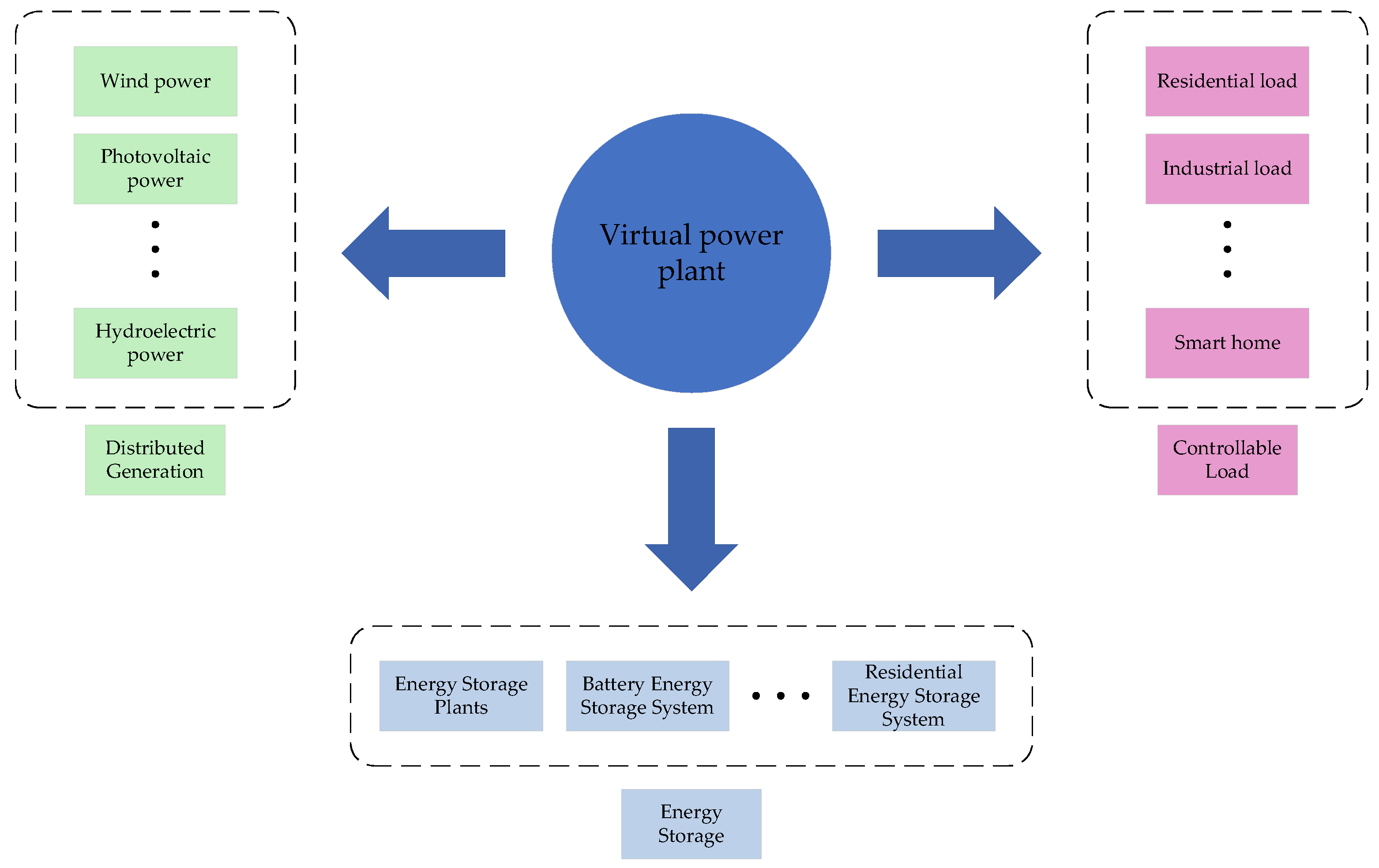
Figure 2.
The structure of LSTM.
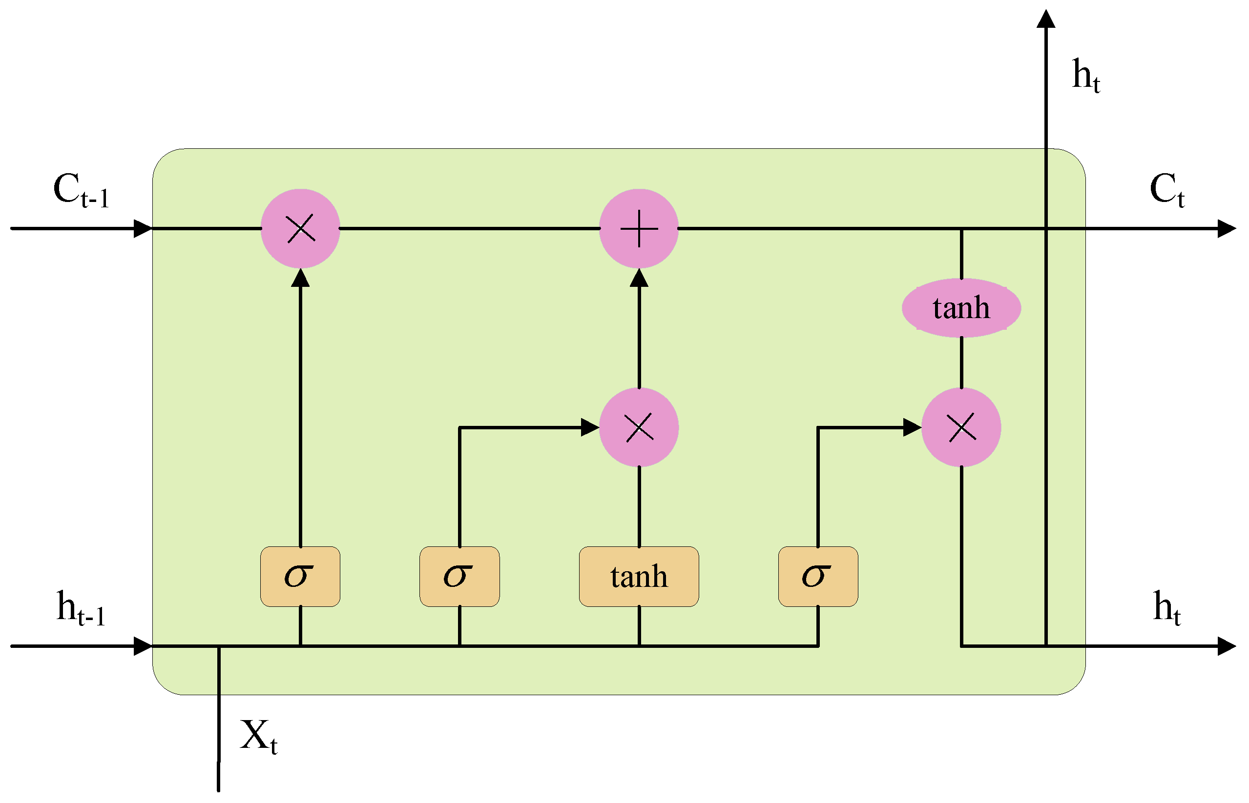
Figure 3.
The structure of BiLSTM.
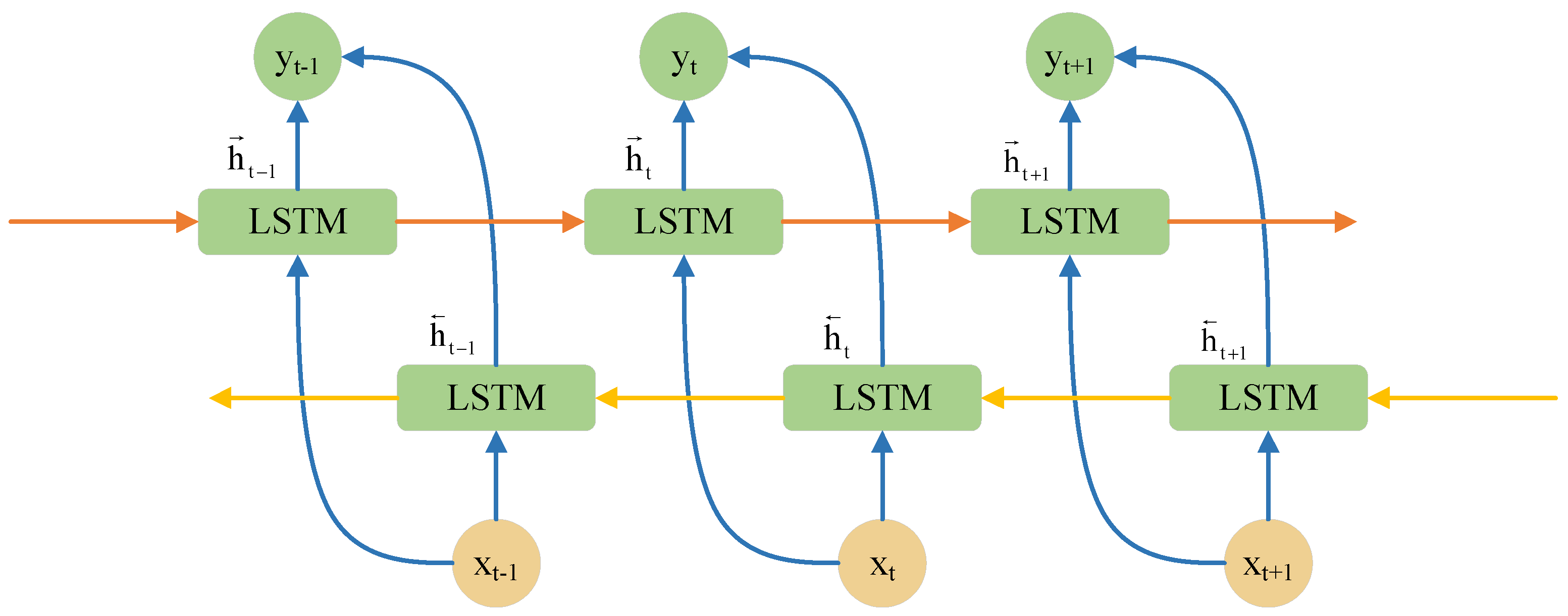
Figure 4.
The structure of Efficient self-attention mechanism.
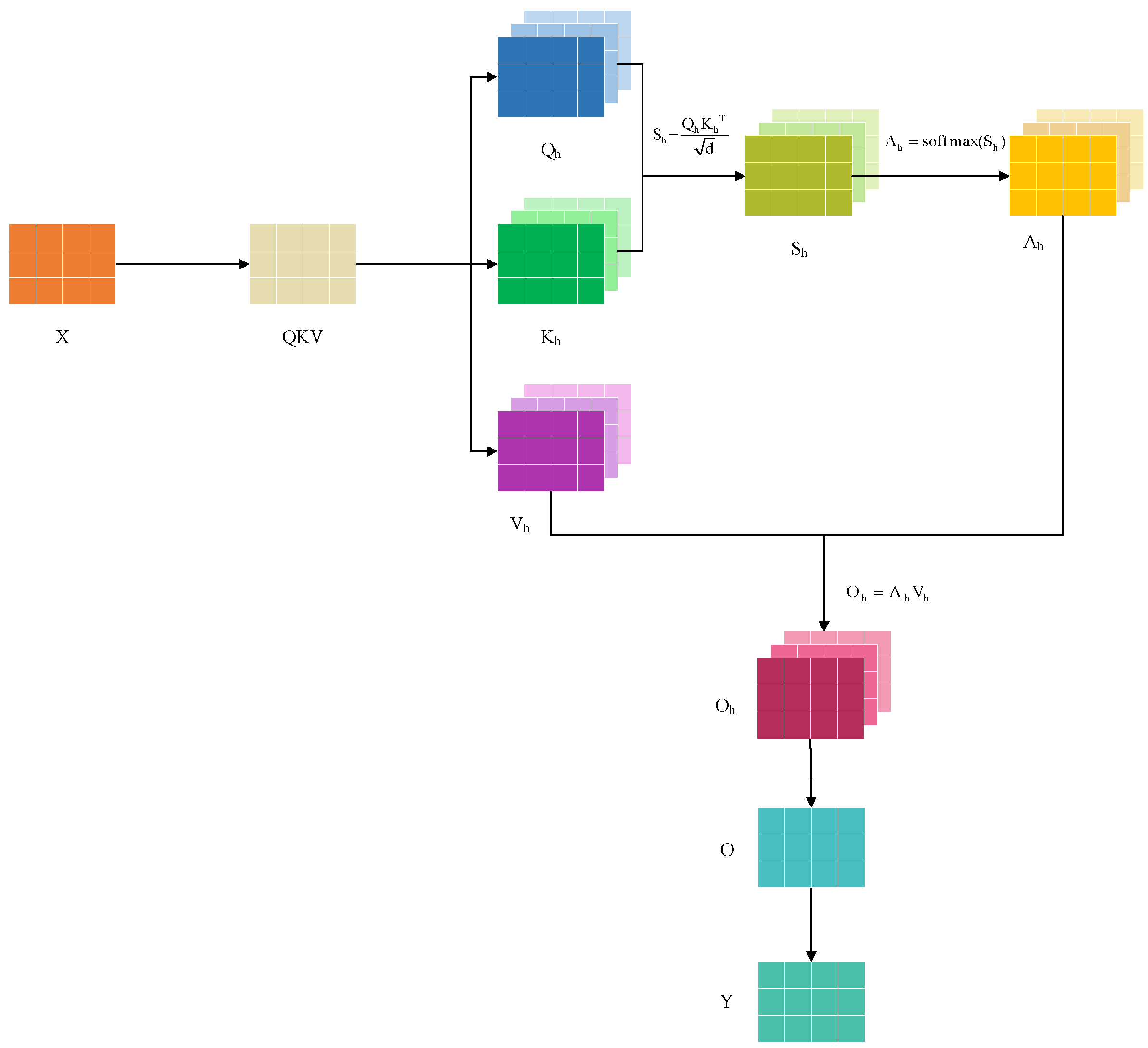
Figure 5.
The frame of Efficient self-attention mechanism.
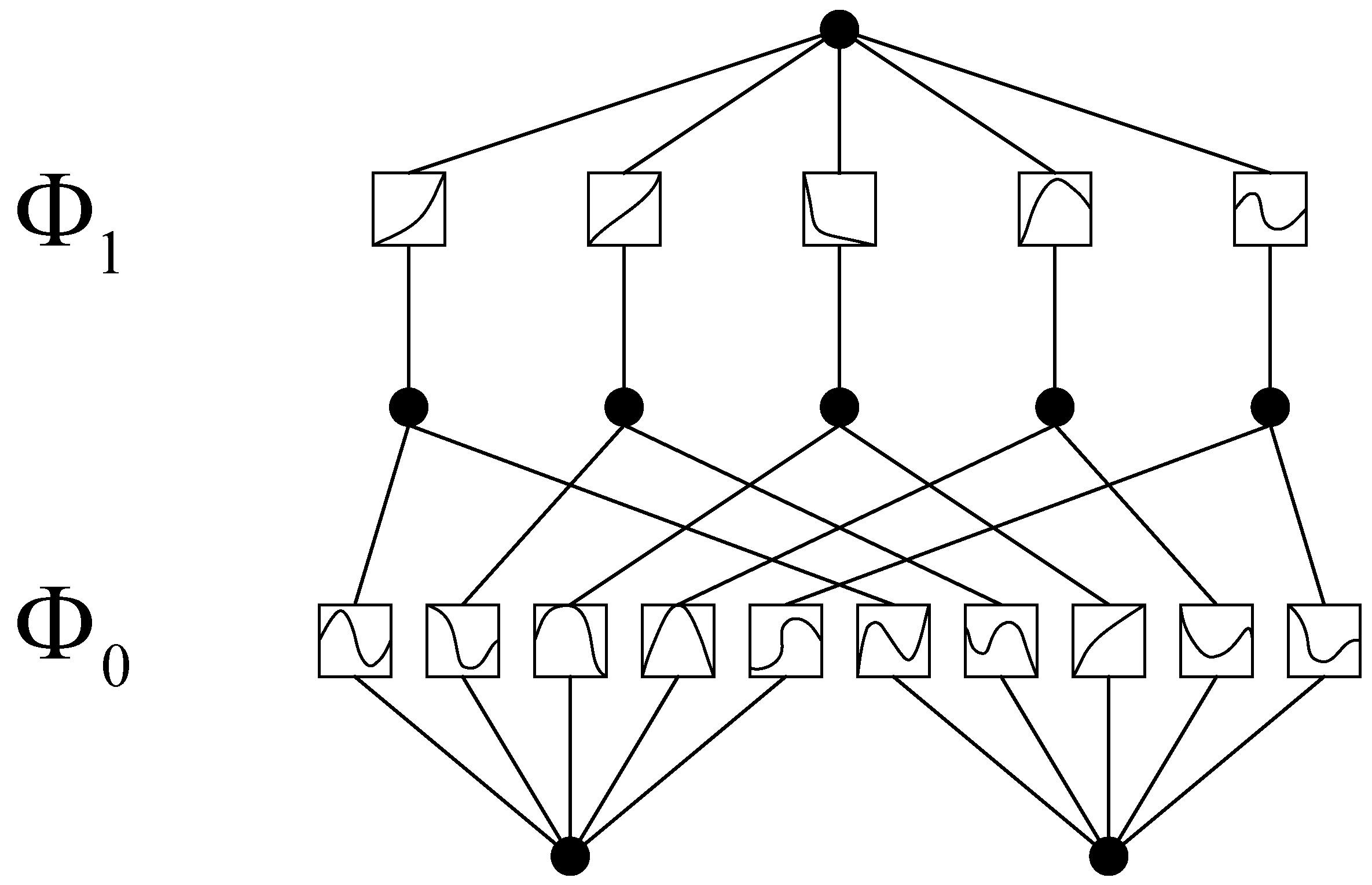
Figure 6.
The structure of BiLSTM-Att-KAN model.
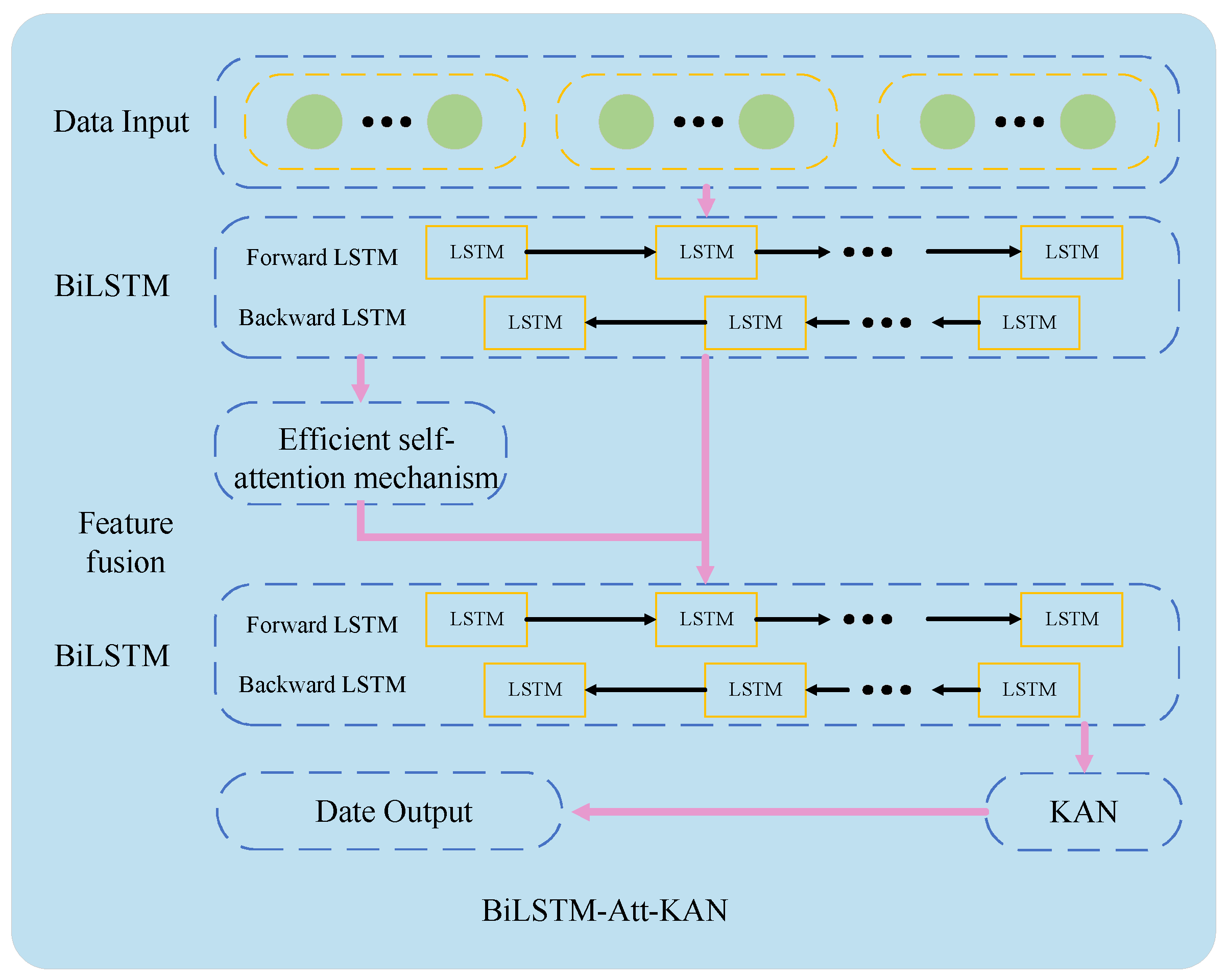
Figure 7.
Flowchart of the integrated forecasting model.

Figure 8.
Electrical load sample points.
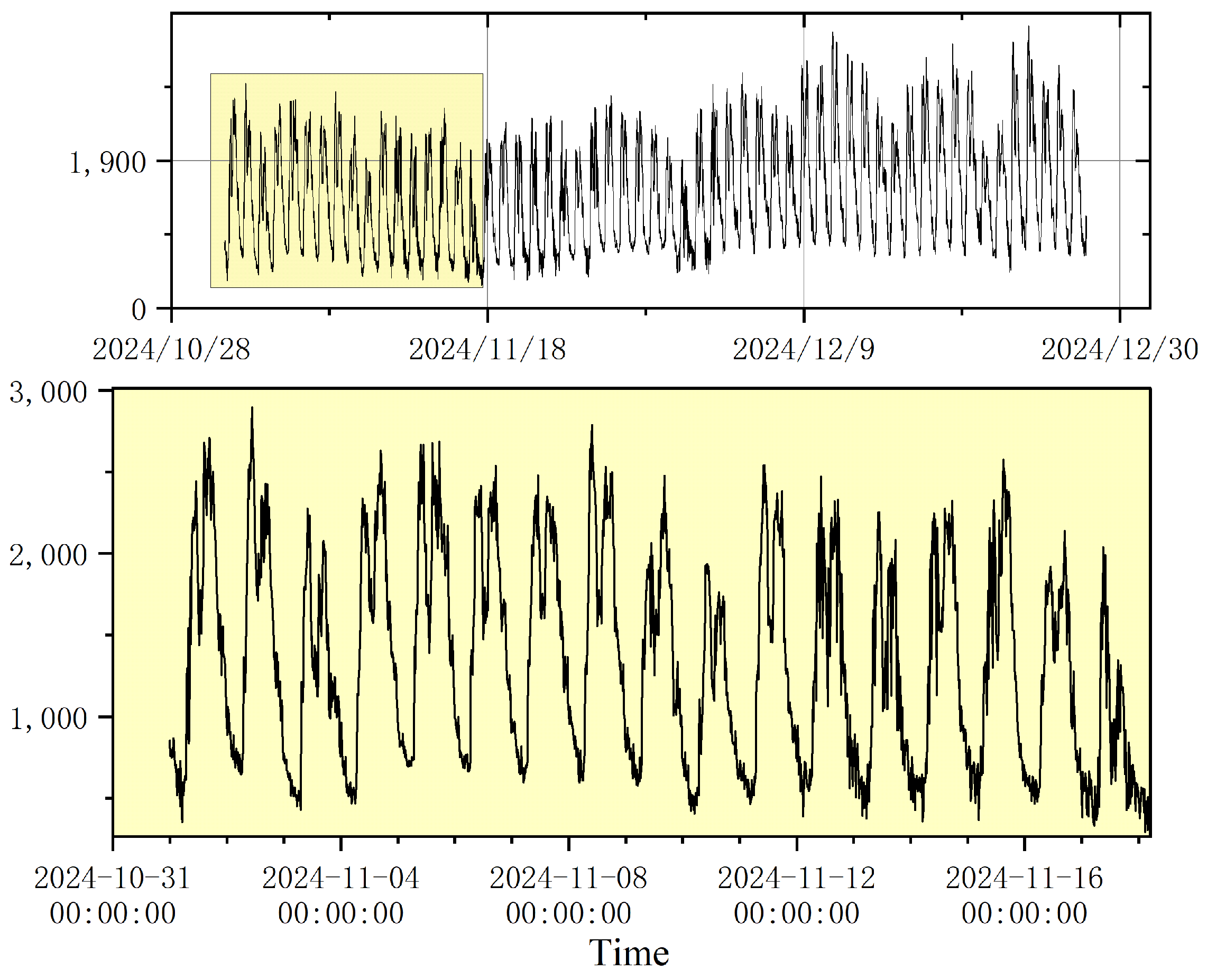
Figure 9.
Feature encoding for (a) Weekday encoding, (b) Daytime encoding.
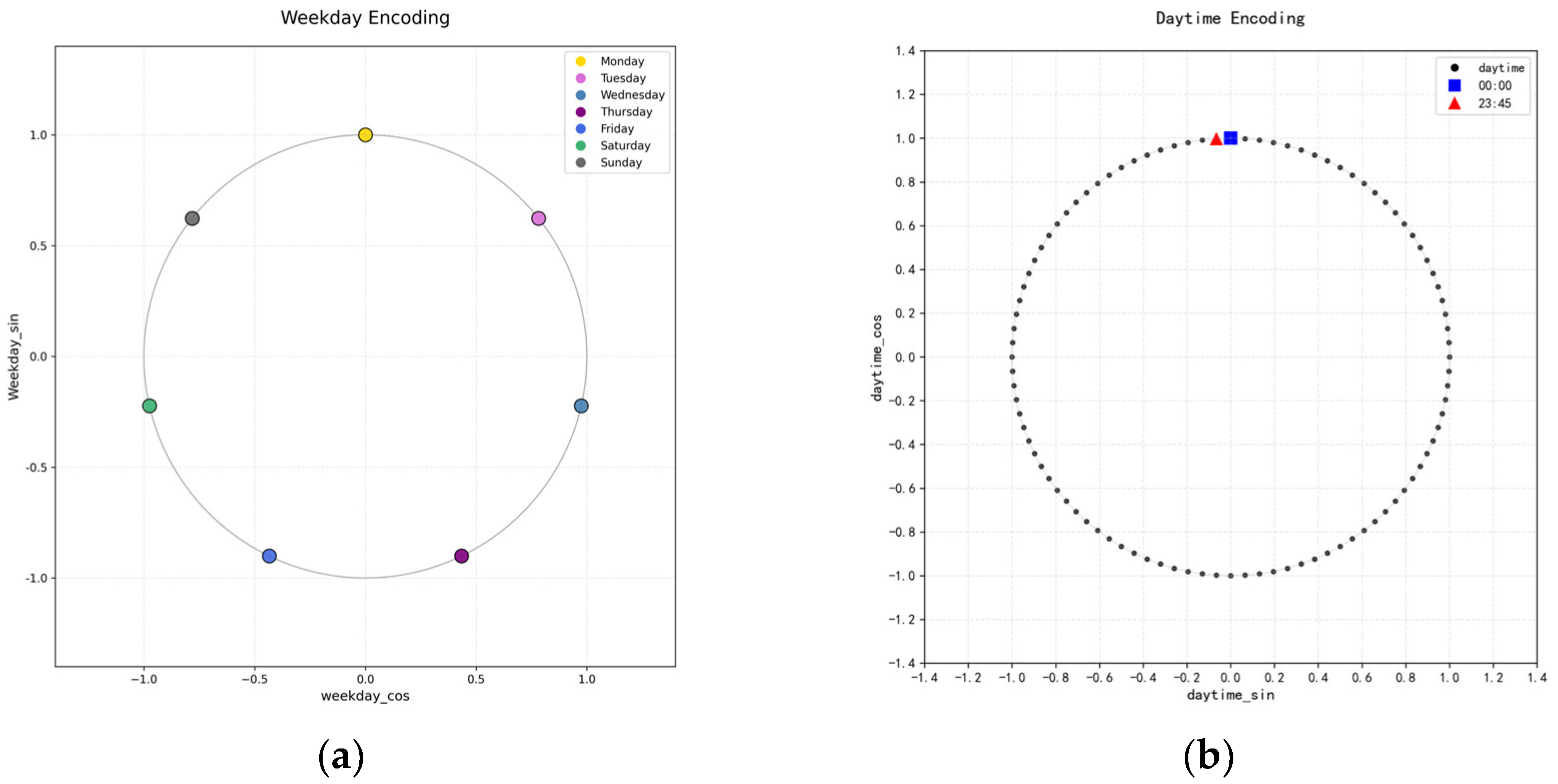
Figure 10.
Forecasting results for different models.

Figure 11.
Forecasting results for ablation experiments.
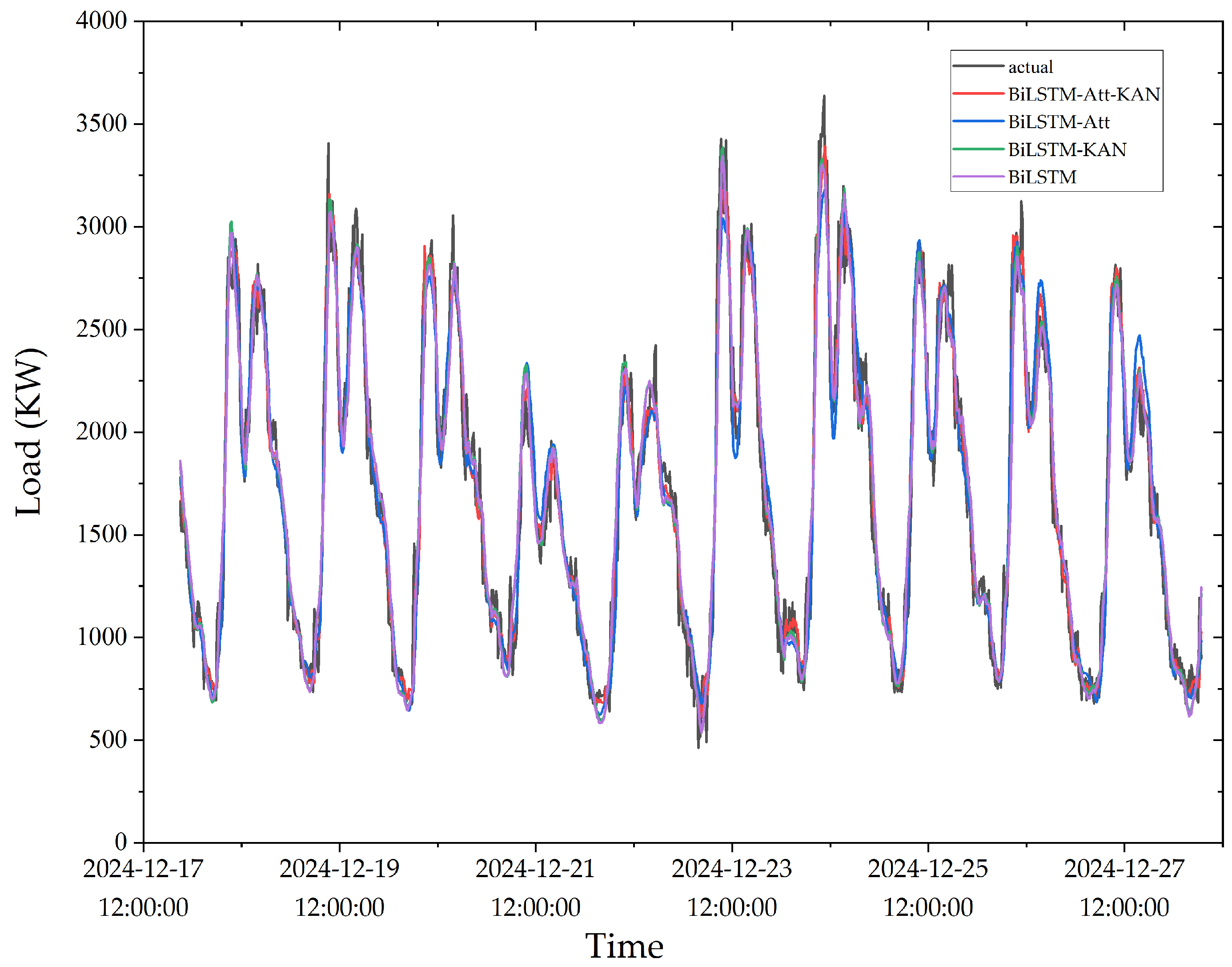
Figure 12.
Forecasting results for different feature inputs.
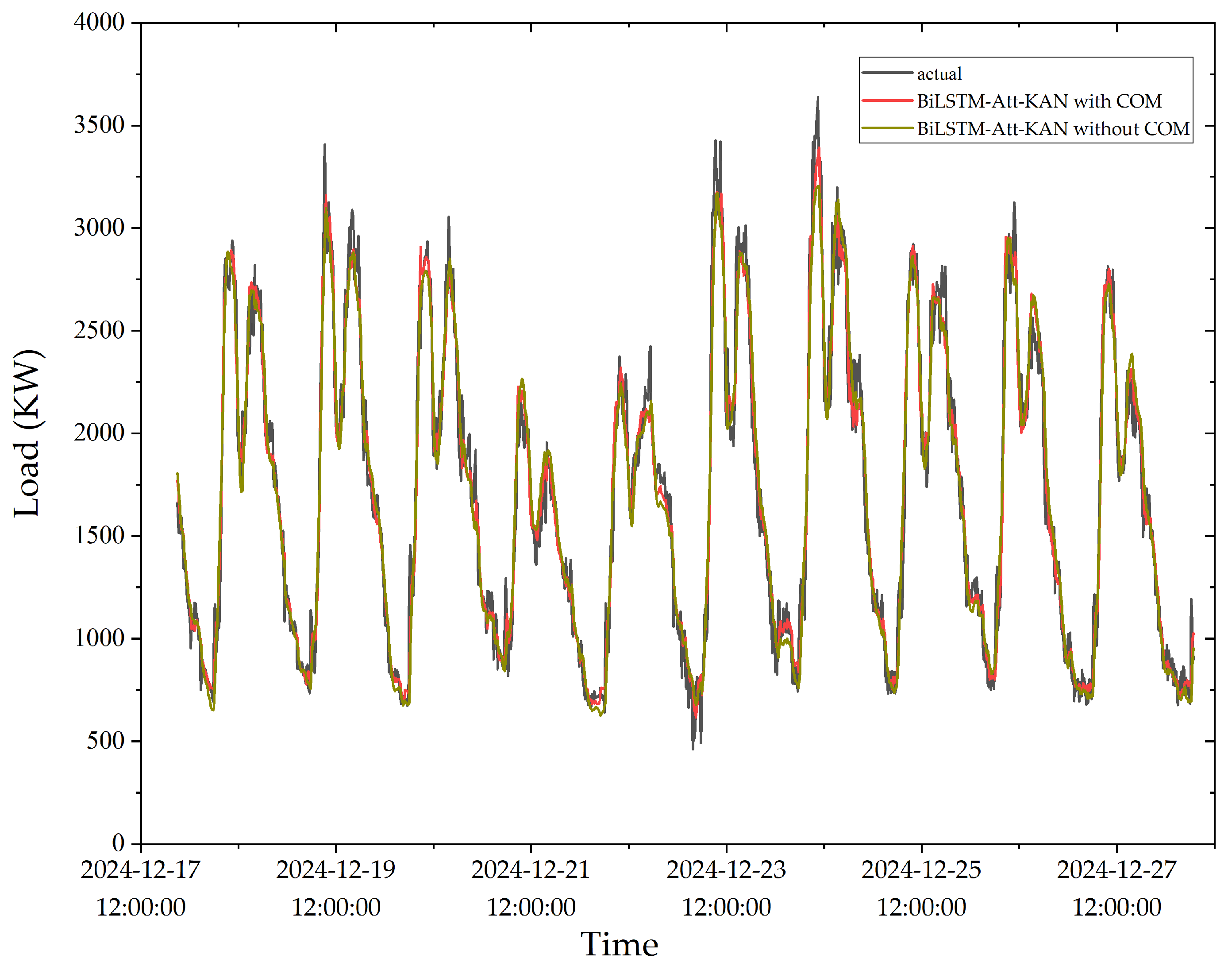
Figure 13.
Box plot of relative errors.
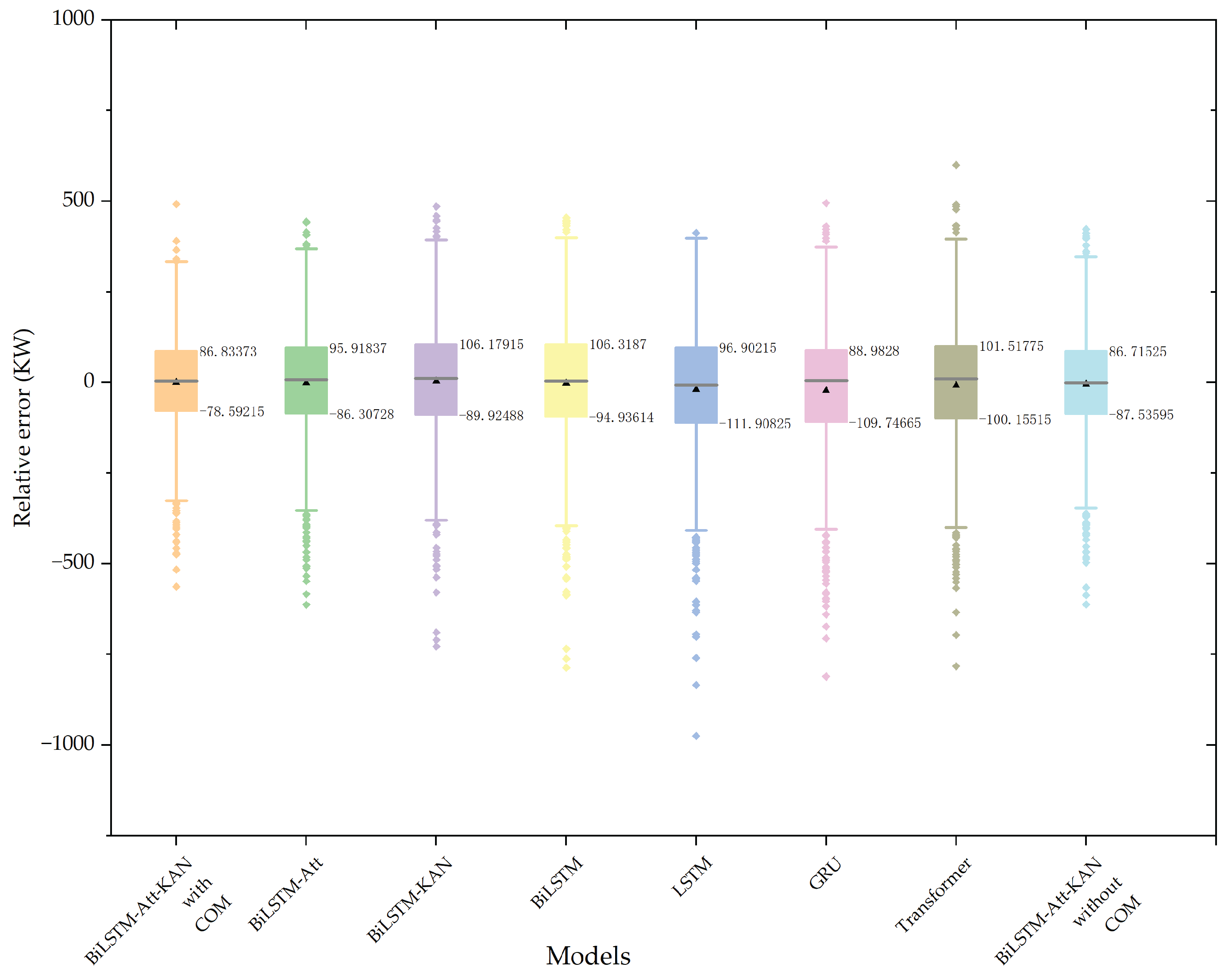

Table 1.
Forecasting results for different models.
| Models | RMSE | MAE | R2 |
|---|---|---|---|
| BiLSTM-Att-KAN | 141.403 | 106.687 | 0.962 |
| BiLSTM | 172.957 | 130.656 | 0.944 |
| LSTM | 181.989 | 136.529 | 0.938 |
| GRU | 182.701 | 133.692 | 0.937 |
| Transformer | 174.614 | 132.177 | 0.943 |
Table 2.
Forecasting results for ablation experiments.
| Models | RMSE | MAE | R2 |
|---|---|---|---|
| BiLSTM-Att-KAN | 141.403 | 106.687 | 0.962 |
| BiLSTM-Att | 159.029 | 119.926 | 0.952 |
| BiLSTM-KAN | 172.802 | 128.731 | 0.951 |
| BiLSTM | 172.957 | 130.656 | 0.944 |
Table 3.
Forecasting results for different feature inputs.
| RMSE | MAE | R2 | |
|---|---|---|---|
| With COM encoding | 141.403 | 106.687 | 0.962 |
| Without COM encoding | 155.009 | 117.076 | 0.955 |
Disclaimer/Publisher’s Note: The statements, opinions and data contained in all publications are solely those of the individual author(s) and contributor(s) and not of MDPI and/or the editor(s). MDPI and/or the editor(s) disclaim responsibility for any injury to people or property resulting from any ideas, methods, instructions or products referred to in the content. |
© 2025 by the authors. Licensee MDPI, Basel, Switzerland. This article is an open access article distributed under the terms and conditions of the Creative Commons Attribution (CC BY) license (http://creativecommons.org/licenses/by/4.0/).
Copyright: This open access article is published under a Creative Commons CC BY 4.0 license, which permit the free download, distribution, and reuse, provided that the author and preprint are cited in any reuse.


