Submitted:
27 December 2024
Posted:
27 December 2024
You are already at the latest version
Abstract
Tasks such as transformer load forecasting, and heavy overload prediction have always been handled in previous work by simple models such as LSTM and XGBoost, which are not able to handle the increasing amount of data in power systems. Recent Foundation models have changed the task-specific modeling approach in time series analysis, they can scaling up to large time series variables and datasets across domains, however the simple pre-training setting makes it unsuitable for complex downstream tasks. To address this problem, this paper proposes the FreqMixer framework for adapting recently proposed time series foundation models to complex tasks in power scenarios, such as the task of predicting transformer load fluctuations caused by the Spring Festival returnees. Experiments demonstrate that the FreqMixer large model is able to adapt to a variety of downstream tasks, obtaining optimal performance in tasks such as overload prediction and load rate prediction (23.65% MAPE reduction, as well as 87% Recall improvement and 72% Precision improvement), while being able to memorize all the large amount of transformer data in a parametrically efficient manner (0.4%) for better performance.
Keywords:
transformer load forecasting
; Parameter Efficient Fine-Tuning
; Multitask Learning
; foundation model
; Spectral Analysis
; time series forecasting
1. Introduction
Accurate load forecasting is critical for the safe operation and maintenance of transformers, preventing overloads and extending equipment life. Load forecasting models help identify potential overload risks and take preventive measures to ensure a balance between supply and demand, reduce energy waste and optimize power dispatch. At the same time, it supports trading decisions in the electricity market, improves grid efficiency and reliability, and reduces overall costs [1,2,3,4]. However, due to the nonlinear relationship between power load and factors such as weather, economic conditions, and population changes, predicting transformer load remains highly complex. Moreover, special events, such as the Spring Festival, can lead to sudden spikes in electricity demand, especially in rural areas, potentially resulting in overloads and voltage instability.
Traditional forecasting methods often rely on time series classification or short-term prediction algorithms [5,6,7,8,9,10], typically combining LSTM and XGBoost [11,12,13,14,15]. While XGBoost requires extensive feature engineering, LSTM suffers from issues like error accumulation in long-term predictions and difficulty in modeling long-distance dependencies. Moreover, these models struggle with large datasets and fail to provide fine-grained insights into “which overloaded when.”
Recent research has enhanced Transformer and MLP architectures to handle time series’ unique properties, such as non-stationarity [16,17,18], periodicity [19], multi-scale characteristics [20,21,22], and trends [23,24,25]. These models effectively address error accumulation and long-range dependencies, with applications in fields like finance [26,27,28,29], energy [30,31,32], transportation [33,34,35], environment [36,37], and industry [38,39,40]. While these models are efficient and fast to train, they struggle with scaling. Modeling thousands of transformers simultaneously can lead to overfitting and resource-heavy computations, making individual transformer models more practical but increasing maintenance burdens.
Foundation Models (FMs) pre-trained on large-scale time series data aim to address these challenges [41,42,43,44,45,46]. FMs offer generalization and can manage tasks involving thousands of transformers, but they are not always suited for complex real-world time series problems. For example, predicting load surges during the Spring Festival requires ultra-long-range dependency modeling, as current loads depend on historical patterns from previous years. This challenge is compounded by the need to incorporate covariates like temperature and population movement, which FMs typically struggle with in pre-training and require careful fine-tuning to integrate.
To overcome the limitations of Foundation Models (FM) and enhance load forecasting, we propose the FreqMixer model, a novel approach for power load forecasting. FreqMixer integrates covariate learning and frequency-domain learning within a multitask fine-tuning framework, improving forecasting accuracy, particularly in special event scenarios like the Spring Festival. Our contributions are as follows:
- We design a Side Network utilizing the PEFT (Parameter Efficient Fine-Tuning) method with covariates to address long-term dependencies. Ablation experiments show that Side Net outperforms traditional methods like full trimming, head trimming, adapter, and LoRA in both time and frequency domains.
- We introduce frequency-domain features combined with PEFT during fine-tuning, enhancing model generalization with fewer parameters and improving performance in diverse scenarios.
- We implement a multi-task learning framework to boost model generalization in Smart Grid Management, mitigating overfitting by leveraging complementary knowledge across tasks, resulting in improved performance across multiple tasks.
2. Related Work
2.1. Foundation Models for Time Series Analysis
In recent years, significant progress has been made in time series forecasting models, particularly in pre-training and cross-domain forecasting for large-scale data. The Lag-Llama [47] model, a decoder-based Transformer, enhances zero-point forecasting by using lags as covariates, effectively capturing long-range dependencies. TimeGPT-1 [45], an encoder-decoder Transformer, improves zero-point prediction efficiency and generalization across domains. TTMs [41], based on TSMixer [48], offer a general framework for multi-domain forecasting without relying on domain-specific data. TimesFM [42], like Lag-Llama, focuses on lag-based pre-training for zero-point prediction. Moirai [44], a masked encoder model trained on the LOTSA dataset (27 billion observations), excels in large-scale, cross-domain forecasting. LLM4TS [49] and TEMPO [50] leverage fine-tuning of GPT-2 for time series forecasting, showing LLMs’ potential in predicting non-linguistic data. LLMTime [51] introduces labeling strategies to enhance zero-point prediction, while Time-LLM [46] integrates text and time series data, increasing flexibility without additional computational cost. Timer [43] and UniTS [52] further develop generalized architectures for multi-task time series analysis.
These models demonstrate the power of Transformer- and LLM-based architectures in time series forecasting and cross-domain applications. However, foundational models focus on generalized pre-training, often lacking comprehensive support for covariates and efficient adaptation to downstream tasks. The challenge remains in effectively integrating task-specific covariates during fine-tuning to meet task requirements.
2.2. Parameter Efficient Fine-Tuning
The most straightforward Parameter Efficient Fine-Tuning (PEFT) method involves modifying a specific subset of parameters in the FM, such as bias and layer specifications, which are critical for downstream tasks. Linear Probe [53] introduces a linear layer on top of the FM as a classifier, freezing FM parameters to explore pre-training capabilities and serving as a baseline for PEFT methods. BitFit [54] shows that optimizing only the bias terms is effective, while DP-BiTFiT [55] focuses on bias terms and scaling factors in specific layers, improving training speed and reducing storage costs. The adapter [56], first used in NLP and later in computer vision (CV), is extended by AdaptFormer [57], which demonstrates the effectiveness of parallel adapter insertion in vision tasks. LoRA [58] approximates weight updates by injecting a low-rank matrix, targeting attention queries and value projection matrices.
Side-Tuning [59] offers a different PEFT approach by employing an independent side network in parallel with the FM, while SAN [60] uses a two-branch side-adapter for mask proposal and attentional bias. ViT-Adapter [61] integrates spatial priors and feature interaction in Visual Transformers, particularly suited for intensive prediction tasks. LST [62] reduces GPU memory consumption by separating trainable parameters from the backbone using a small Transformer, and DTL [63] designs a compact side network for ViT to improve parameter and memory efficiency.
Compared to Linear Probe, adapters, and LoRA, sidetuning introduces prior knowledge and covariates, offering more adaptability to downstream tasks while maintaining PEFT efficiency.
2.3. Multitask Learning
Multi-task learning (MTL) enhances task-specific performance by training models on multiple related tasks simultaneously, capturing generalized and complementary knowledge. It expands datasets and reduces overfitting by incorporating unsupervised or self-supervised tasks, making it ideal for data-scarce scenarios. MTL improves model performance through shared knowledge across tasks and enables transfer learning by adding task-specific parameters, suitable for delay-sensitive applications. Models like MultiNet [64], Mult [65], and UniT [66] use shared backbone networks and task-specific heads, with encoders learning a generic representation and task heads making predictions.
A key challenge in MTL is balancing the learning of all tasks to prevent one task from dominating. Uncertainty Weighting [67] addresses this by optimizing model weights and noise parameters, giving lower weights to tasks with higher uncertainty. GradNorm [68] balances the learning rates of tasks by normalizing gradient magnitudes, ensuring stable training. Dynamic Weight Averaging (DWA) [69] adjusts task weights dynamically, while Dynamic Task Prioritization (DTP) [70] prioritizes tasks with higher losses. MGDA [71] treats MTL as a multi-objective optimization problem, seeking a Pareto optimal solution for task balance.
In smart grid tasks like station load forecasting and overload prediction, MTL improves accuracy, reduces overfitting, enhances robustness, and handles multiple tasks within a single model.
3. Methodologies of FreqMixer
3.1. Problem Formulation & End-to-End multitask Finetuning
We evaluate our approach on three time series tasks: forecasting, classification, and multi-task learning. Each task has its own challenges, from predicting future values to classifying time series and managing multiple tasks simultaneously. Below, we outline the key aspects for each task, including quantile loss for forecasting, cross-entropy loss for classification, and GradNorm for balancing multi-task learning.
Time Series Forecasting Task. We define a multivariate time series as , where T is the time series length, and C is the number of channels (features). The task is a sequence-to-sequence prediction: given a history sequence x, we predict the future sequence using a model , resulting in a forecast , where H is the forecast horizon.
We train the model by minimizing the quantile loss (MQLoss), which measures asymmetrical errors between y and for a given quantile q:
where . The parameter q adjusts the weight for over- or under-predictions, making the loss suitable for capturing uncertainties.
Time Series Classification Task. A multivariate time series is represented as , where T is the length of the time series and C is the number of channels (or variates). In the BizITObs domain, these channels include both business KPIs and IT events. The classification task aims to predict a class label from a sequence x using a model , resulting in a prediction , where K is the number of predefined classes.
The model is trained by minimizing the Cross-Entropy Loss:
where is the true label (one-hot encoded), is the predicted probability, and is the weight for class i, typically balancing class frequency: with N being the total number of samples and the number of samples in class i. This loss encourages the model to correctly classify by aligning the predicted probabilities with the true label distribution.
Multi-Task Learning with GradNorm for Task Balancing. In multi-task learning (MTL), we predict multiple related tasks simultaneously from a univariate time series , where T is the time series length. For each task , the model predicts target sequences , with being the output length for task k.
The model outputs a set of predictions for all tasks:
where are the predicted outputs for the tasks. A key challenge in MTL is balancing the learning speed of different tasks, which may have varying scales and difficulties. GradNorm addresses this by adjusting task weights to equalize the gradient norms of different tasks during training, ensuring all tasks learn at similar rates.
The total loss is a weighted sum of individual task losses:
where is a learnable weight, and is the loss for task k. GradNorm dynamically adjusts based on the gradient norms to balance training by equalizing the normalized gradient norms of all tasks. This prevents any single task from dominating, promoting balanced learning across all tasks.
3.2. Background of TTMs
Our approach builds on the large-scale pre-trained foundation model TTMs. Tiny Time Mixers (TTMs) are compact models (starting from 1 million parameters) designed for efficient transfer learning on publicly available time series datasets. Based on the lightweight TSMixer architecture, TTMs use methods like adaptive chunking, diverse resolution sampling, and resolution prefix tuning to handle multiresolution pre-training with limited capacity. TTMs capture inter-channel correlations and incorporate exogenous signals during fine-tuning, making them highly effective for zero- and few-shot prediction tasks, improving performance by 4%-40% over popular benchmarks while reducing computational requirements. TTMs can even run on CPU-only devices, increasing usability in resource-limited environments. The TTMs workflow consists of two phases:
Pre-training phase: TTMs are trained on public datasets focusing on univariate time series. Multivariate datasets are converted into independent univariate series for preprocessing and backbone network input. Multiresolution pretraining captures temporal dynamics using Mean Square Error (MSE) loss. Multivariate correlation handling is deferred to the fine-tuning phase.
Fine-tuning phase: TTMs adapt to the target domain with zero-, few-, or full-sample prediction. During fine-tuning, the backbone network is frozen, and the decoder handles multivariate tasks by enabling the channel mixer to capture inter-channel correlations.
3.3. End-to-End Multitask Finetuning Framework
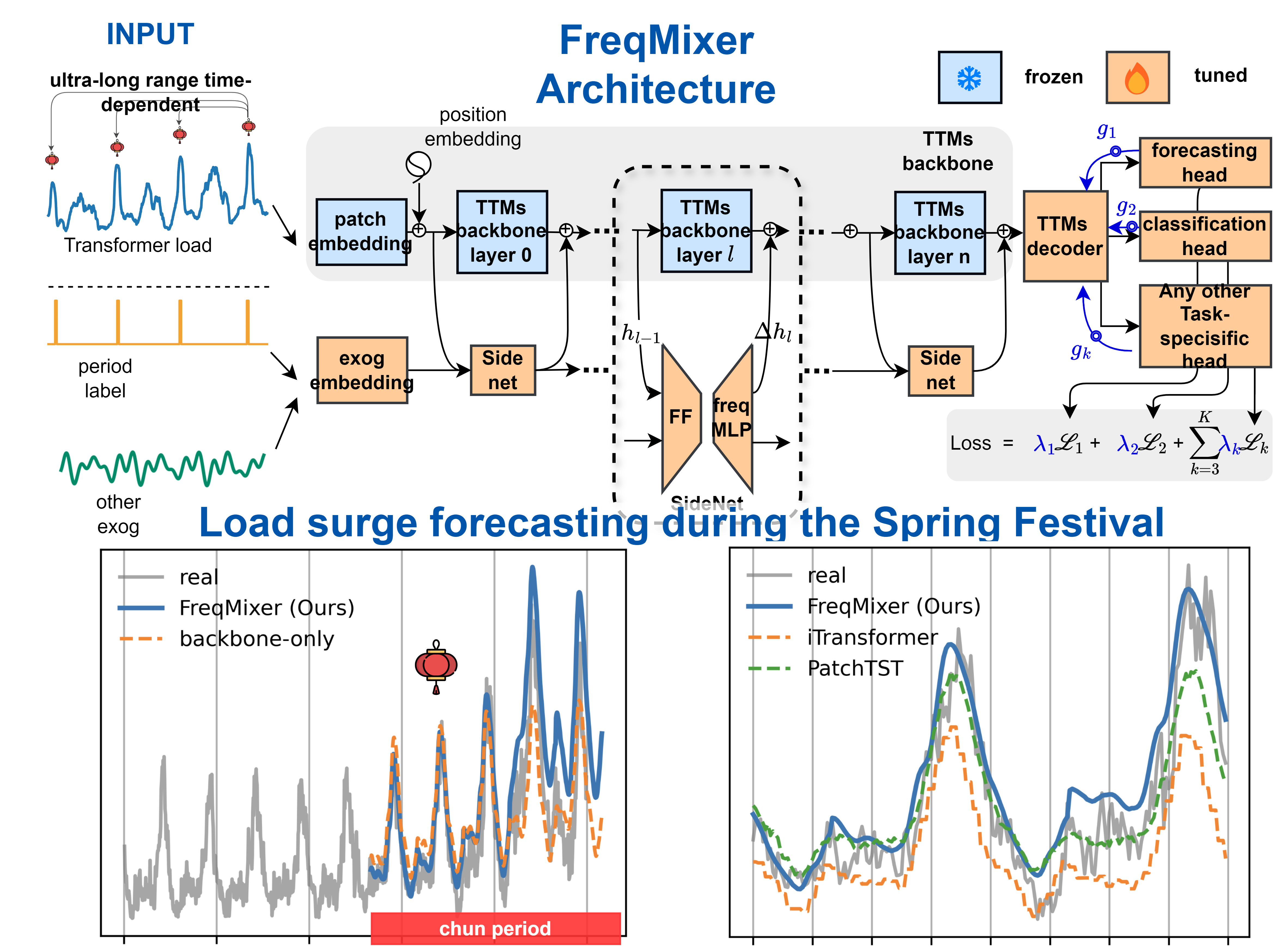
We explore Parameter Efficient Fine-Tuning (PEFT), which aims to surpass full fine-tuning with minimal parameter changes, allowing the model to efficiently adapt to new tasks while preserving the knowledge in the frozen backbone network. The backbone, responsible for processing low-level or generic features learned during pre-training, remains unchanged. Instead, fine-tuning focuses on the added companion network, the decoder, and the multi-task prediction head, enabling adaptation to the transformer load prediction task. Our fine-tuned module includes a FeedForward (FF) module and a frequency domain learning module, FreqMLP, as shown in Figure 1.
Embedding. The model input consists of the historical window of load data , future covariates , and other historical covariates, such as weather and population flow data . The historical window passes through the embedding layer of the Backbone, resulting in an embedding , where . In details, at the i-th layer of the Backbone, the patch splitting block of the Backbone reshapes the input from the previous layer into the current layer’s input , where . This increases the number of patches by -fold and reduces the patch size by the same -fold. The future covariates and historical covariates are transformed through linear layers, where the historical covariates are mapped via the weight matrix , and the future covariates are mapped via the weight matrix . To allow interaction between each channel of the historical variables and covariates, we replicate the covariate embeddings C times and concatenate them with xalong the last dimension, resulting in an embedding .
FeedForward. In the feedforward layer, the input embedding vector e is first mapped to a lower-dimensional space via the weight matrix , followed by a nonlinear activation function. Then, the mapped vector is transformed back to the original dimension via the weight matrix .
FreqMLP. Previous work [72] found that the frequency domain MLP learning mode is favorable for timing prediction. MLP in frequency-domain learning has two main advantages: first, it captures the global dependencies of the signal through the spectrum, which leads to a better understanding of the overall structure of the data; and second, it improves the learning efficiency and reduces the noise interference by concentrating the energy of the signal in the key parts of the frequency domain. Specifically, the input vector is transformed into the frequency domain via a Fourier transform, resulting in a complex representation with real and imaginary parts. The real and imaginary components are then projected to a lower-dimensional space using separate weight matrices , effectively reducing the dimensionality of the input. After projection, the real and imaginary parts are activated using a non-linear function such as ReLU and normalized, followed by dropout to prevent overfitting. The resulting low-dimensional vectors are then projected back to the original dimension using the weight matrix . Subsequently, a sparse activation function (e.g., Softshrink) is applied to the combined real and imaginary parts to retain the most relevant features while reducing redundancy. Finally, the data is transformed back to the time domain via an inverse Fourier transform, yielding the processed embedding , which models the relationship between the load ratio and the covariates.
SideNet. In each layer of the SideNet, the output of the corresponding layer in the backbone network is incorporated to refine the hidden state. Specifically, the process is as follows: Let denote the output of the l-th layer in the backbone network, where , with being the input from the previous layer. The SideNet then computes a residual update and an auxiliary embedding by processing the concatenation of the backbone’s hidden state and the embedding from the previous layer of the SideNet, , as follows:
The hidden state for the current layer is then updated by adding the residual to the previous hidden state, yielding the final output for the current layer:
This process allows the SideNet to iteratively refine the hidden state by incorporating information from both the backbone and auxiliary features at each layer, enhancing the model’s representation power and capacity to learn complex relationships between the inputs.
Task-specific Head. After the embedding passes through the decoder, its shape remains unchanged, serving as a shared representation for all tasks. This shared representation is then fed into multiple task-specific heads. For the regression task, the shared representation is processed by a linear layer with a weight matrix , producing the regression output as , where H represents the output dimension for the regression task. Similarly, for the classification task, the shared representation is fed into a classification head with a weight matrix , yielding the classification logits as , where num_class represents the number of classes in the classification task. These task-specific heads allow the model to adapt the shared representation h to different tasks, such as regression and classification, while maintaining a consistent dimensionality throughout.
4. Experiments
4.1. Data
For experimental purposes, we selected electric load data from 2021 to present (2024-September) for more than 160 transformers in a region of southern China. The data were sampled every 15 minutes. Each point-in-time data is labeled according to the official rubric for whether it is in a heavy or overloaded state. The data before 2024 is taken as the training set and the data after 2024 is taken as the test set. These transformers have unstable load characteristics during the Chinese New Year period every year due to the homecoming wave, which creates a big obstacle for the management and maintenance of the equipment. All data are normalized by the features of the training set to ensure the stability of training. Due to the sensitive nature of the data, it cannot be publicly disclosed.
4.2. Experimental Setting
To evaluate the performance of our FreqMixer model, we benchmark it against several well-established multivariate time series forecasting methods. We focus on comparing FreqMixer to deep learning models and mixer models, excluding traditional approaches like XGBoost and ARIMA, as they struggle with complex features and large-scale data.
Forecasting Benchmarks. We compare FreqMixer with various multivariate time series prediction models: (i) mixer models (including FreqMixer and TTMs), (ii) deep learning models such as PatchTST [22], DLinear [25], iTransformer [73], tsMixer [48], and timemixer [74], and (iii) LSTM+MLP [75], MLP [76]. We do not include traditional methods like XGBoost or ARIMA due to their limitations in capturing complex time series patterns, especially for long-term prediction.
Model Configuration. All models were trained with a context length and prediction length , except for FreqMixer, which uses autoregression to predict 96 steps at a time. For FreqMixer, the batch size was and the hidden feature size for the SideNet was 32. Baseline models were implemented using the Neuralforecast and Time Series libraries with recommended hyperparameters. All models were trained with early stopping based on validation performance, using a quantile loss function (MQloss) with a quantile of 0.8. Our training environment included 72-core CPUs, 256GB of RAM, and two H100 80GB GPUs.
Metrics. We evaluate performance using regression metrics (MSE, MAE, MAPE) and classification metrics (Accuracy, Precision, Recall, F1-score). Classification metrics are particularly important for transformer load prediction tasks, as they reflect whether the predicted values correctly indicate the equipment’s operational state, such as overload conditions. We determine overloads by checking if the load rate exceeds a predefined threshold.
4.3. Load Forecasting in 2024 Spring Festival
In this section, we demonstrate the potential of the model for load factor prediction through various empirical evidence.
Load Forecasting. In our experiments, we compared the FreqMixer models with current benchmark models, using data from the past 5 days to predict the load for the next 3 days. To fully evaluate model performance, we assessed each model at different lead times. Table 1 clearly shows that FreqMixer significantly outperforms traditional LSTM hybrid methods and MLP schemes in power load forecasting, particularly for multi-day lead time predictions.
Specifically, FreqMixer achieves a 24% reduction in MAPE, an 87% improvement in recall, and a 72% increase in accuracy. These improvements highlight that FreqMixer not only better captures the relationship between historical and future data, but also excels at handling complex time-dependent features. Notably, FreqMixer achieves 3.5 times the recall of the SOTA benchmark and doubles the Precision when the lead time is 3 days. These advancements are largely due to FreqMixer’s ability to model long-range dependencies, overcoming the limitations of traditional models, and delivering more consistent and accurate results, especially in capturing complex long-distance dependencies. Figure 2 shows the forecasting results during the Spring Festival, with a load surge observed in a transformer in southern China (a), comparing the performance of FreqMixer with other methods.
These results demonstrate that FreqMixer not only improves prediction accuracy in power load forecasting, but also effectively handles the impact of special events, like the Chinese New Year, on transformer loads. Leveraging the power of a large model and multidimensional covariates, FreqMixer shows strong performance in addressing long-distance dependencies and complex time series forecasting tasks.
Overload Prediction. In this section, we show the applicability of the pre-trained model to different types of downstream tasks (i.e., ). We use 5 days of historical data to predict whether the next day’s will be heavily overloaded or not. As shown in Table 2, our method significantly reduces the false alarm rate and improves the accuracy of the prediction compared to other baseline methods. On the one hand, this is due to the fact that our method is better able to capture the complex relationship between historical load data and future heavy overload events; on the other hand, it is the fact that the pre-training step helps to improve the generalization to multiple downstream tasks, highlighting the potential of the time series base model.
4.4. Ablation Study
To better understand the effectiveness of our proposed model and its components, we conducted a series of ablation studies. These experiments were designed to isolate and evaluate the contributions of different architectural choices, including the use of the SideNet module, covariate handling strategies, and the fine-tuning approaches. In the following sections, we present the results of these ablation experiments to highlight the importance of each design decision in improving model performance and parametric efficiency.
Applicability to Multiple Downstream Tasks. We tested various fine-tuned architectures in both multitasking and single-tasking scenarios and justified our design. We used load rate data from 10 transformers for testing and evaluated the performance of the model in a load prediction task. Table 3 shows the experimental results, where Full represents full fine-tuning, head represents only the task head being fine-tuned, and adapter and lora as well as side net all use our proposed SideNet module to support covariates, with the difference being in the different locations and whether or not to pass the covariate as a state quantity with the network layer. Full, head, and lora do not pass covariates to the next layer; they use the same covariate embedding for each layer. Experimental results demonstrate that this approach is suboptimal, due to the fact that the covariate embeddings of adapter and SideNet allow for a more abstract representation at deeper layers. Finally, the parallel SideNet shows the best performance over the serial adapter in both single and multitasking situations. This conclusion is not surprising, as previous work [57] has demonstrated that parallel structures always have better performance for the same structure.
Parametric Efficiency. The parametric efficiency of our approach cannot be captured in this experiment because the TTMs pre-training model itself is small. We tested the efficiency of the fine-tuning module on the pre-trained Transformer Timer by performing a temporal prediction task on the ETTh1 [77] dataset, using 512 historical sequences to predict 96 long sequences. We use the FF-only module and the FreqMLP-only module as well as the hybrid module. The experimental results in Table 4 demonstrate that when fine-tuning in the frequency domain, performance can be obtained with about 1/100 of the parameters over the full amount of fine-tuning methods. Despite the higher efficiency of FreqMLP-only, the reason we still need hybrid is that FreqMLP cannot handle discontinuous signals, such as step signals.
5. Conclusions
In this paper, we propose the FreqMixer framework for adapting time-series foundation models to power-related tasks. Through extensive experiments, we show that using covariates for downstream tasks achieves a 20% reduction in MAPE, 80% recall improvement, and 70% precision enhancement in transformer load prediction during Chinese New Year. We demonstrate that incorporating frequency-domain features during fine-tuning improves efficiency, with our module fine-tuned on Timer achieving optimal performance on the ETTh1 dataset using only 1/232 of the parameters. Additionally, multi-task fine-tuning adapts a single model for multiple tasks, improving recall by 8% and precision by 100% in load classification. Our next steps includes real-time system monitoring and addressing system limitations.
Author Contributions
Conceptualization, Yikai Hou and Chao Ma; methodology, Yikai Hou and Chao Ma; software, Xiang Li; validation, Yikai Hou, Chao Ma, and Yinggang Sun; formal analysis, Yikai Hou; investigation, Yikai Hou and Xiang Li; resources, Chao Ma and Haining Yu; data curation, Xiang Li; writing—original draft preparation, Yikai Hou; writing—review and editing, Yikai Hou and Chao Ma; visualization, Yikai Hou; supervision, Chao Ma; project administration, Chao Ma; funding acquisition, Zhou Fang. All authors have read and agreed to the published version of the manuscript.
Funding
This research was funded by National Natural Science Foundation, China (No. 62172123), the Key Research and Development Program of Heilongjiang (Grant No. 2022ZX01A36), the Special projects for the central government to guide the development of local science and technology, China (No. ZY20B11), the Harbin Manufacturing Technology Innovation Talent Project (No. CXRC20221104236), Natural Science Foundation of Heilongjiang Province of China (Grant No. YQ2021F007).
Institutional Review Board Statement
Not applicable.
Informed Consent Statement
Not applicable.
Data Availability Statement
Data cannot be provided due to privacy.
Conflicts of Interest
The authors declare no conflicts of interest
Abbreviations
The following abbreviations are used in this manuscript:
| PEFT | Parameter Efficient Fine-Tuning |
| TTMs | Tiny Time Mixers |
| MTL | Multi-Task Learning |
| FMs | Foundation Models |
References
- Ahmad, N.; Ghadi, Y.; Adnan, M.; Ali, M. Load forecasting techniques for power system: Research challenges and survey. IEEE Access 2022, 10, 71054–71090. [Google Scholar] [CrossRef]
- Nti, I.K.; Teimeh, M.; Nyarko-Boateng, O.; Adekoya, A.F. Electricity load forecasting: a systematic review. Journal of Electrical Systems and Information Technology 2020, 7, 1–19. [Google Scholar] [CrossRef]
- Zhu, J.; Dong, H.; Zheng, W.; Li, S.; Huang, Y.; Xi, L. Review and prospect of data-driven techniques for load forecasting in integrated energy systems. Applied Energy 2022, 321, 119269. [Google Scholar] [CrossRef]
- Haben, S.; Arora, S.; Giasemidis, G.; Voss, M.; Greetham, D.V. Review of low voltage load forecasting: Methods, applications, and recommendations. Applied Energy 2021, 304, 117798. [Google Scholar] [CrossRef]
- Cao, L.; Li, Y.; Zhang, J.; Jiang, Y.; Han, Y.; Wei, J. Electrical load prediction of healthcare buildings through single and ensemble learning. Energy Reports 2020, 6, 2751–2767. [Google Scholar] [CrossRef]
- Khan, A.N.; Iqbal, N.; Ahmad, R.; Kim, D.H. Ensemble prediction approach based on learning to statistical model for efficient building energy consumption management. Symmetry 2021, 13, 405. [Google Scholar] [CrossRef]
- Kong, W.; Dong, Z.Y.; Jia, Y.; Hill, D.J.; Xu, Y.; Zhang, Y. Short-term residential load forecasting based on LSTM recurrent neural network. IEEE transactions on smart grid 2017, 10, 841–851. [Google Scholar] [CrossRef]
- Alhussein, M.; Aurangzeb, K.; Haider, S.I. Hybrid CNN-LSTM model for short-term individual household load forecasting. Ieee Access 2020, 8, 180544–180557. [Google Scholar] [CrossRef]
- Muzaffar, S.; Afshari, A. Short-term load forecasts using LSTM networks. Energy Procedia 2019, 158, 2922–2927. [Google Scholar] [CrossRef]
- Abumohsen, M.; Owda, A.Y.; Owda, M. Electrical load forecasting using LSTM, GRU, and RNN algorithms. Energies 2023, 16, 2283. [Google Scholar] [CrossRef]
- Ma, H.; Yang, P.; Wang, F.; Wang, X.; Yang, D.; Feng, B. Short-Term Heavy Overload Forecasting of Public Transformers Based on Combined LSTM-XGBoost Model. Energies 2023, 16, 1507. [Google Scholar] [CrossRef]
- Wang, Y.; Sun, S.; Chen, X.; Zeng, X.; Kong, Y.; Chen, J.; Guo, Y.; Wang, T. Short-term load forecasting of industrial customers based on SVMD and XGBoost. International Journal of Electrical Power & Energy Systems 2021, 129, 106830. [Google Scholar]
- Deng, X.; Ye, A.; Zhong, J.; Xu, D.; Yang, W.; Song, Z.; Zhang, Z.; Guo, J.; Wang, T.; Tian, Y.; et al. Bagging–XGBoost algorithm based extreme weather identification and short-term load forecasting model. Energy Reports 2022, 8, 8661–8674. [Google Scholar] [CrossRef]
- Yao, X.; Fu, X.; Zong, C. Short-term load forecasting method based on feature preference strategy and LightGBM-XGboost. IEEE Access 2022, 10, 75257–75268. [Google Scholar] [CrossRef]
- Zhang, L.; Jánošík, D. Enhanced short-term load forecasting with hybrid machine learning models: CatBoost and XGBoost approaches. Expert Systems with Applications 2024, 241, 122686. [Google Scholar] [CrossRef]
- Liu, Y.; Wu, H.; Wang, J.; Long, M. Non-stationary transformers: Exploring the stationarity in time series forecasting. Advances in Neural Information Processing Systems 2022, 35, 9881–9893. [Google Scholar]
- Kim, T.; Kim, J.; Tae, Y.; Park, C.; Choi, J.H.; Choo, J. Reversible instance normalization for accurate time-series forecasting against distribution shift. In Proceedings of the International Conference on Learning Representations; 2021. [Google Scholar]
- Ogasawara, E.; Martinez, L.C.; De Oliveira, D.; Zimbrão, G.; Pappa, G.L.; Mattoso, M. Adaptive normalization: A novel data normalization approach for non-stationary time series. In Proceedings of the The 2010 International Joint Conference on Neural Networks (IJCNN). IEEE; 2010; pp. 1–8. [Google Scholar]
- Wu, H.; Hu, T.; Liu, Y.; Zhou, H.; Wang, J.; Long, M. Timesnet: Temporal 2d-variation modeling for general time series analysis. arXiv, 2022; arXiv:2210.02186. [Google Scholar]
- Oreshkin, B.N.; Carpov, D.; Chapados, N.; Bengio, Y. N-BEATS: Neural basis expansion analysis for interpretable time series forecasting. arXiv, 2019; arXiv:1905.10437. [Google Scholar]
- Challu, C.; Olivares, K.G.; Oreshkin, B.N.; Ramirez, F.G.; Canseco, M.M.; Dubrawski, A. Nhits: Neural hierarchical interpolation for time series forecasting. In Proceedings of the Proceedings of the AAAI Conference on Artificial Intelligence; 2023; Vol. 37, pp. 376989–6997. [Google Scholar]
- Nie, Y.; Nguyen, N.H.; Sinthong, P.; Kalagnanam, J. A time series is worth 64 words: Long-term forecasting with transformers. arXiv, 2022; arXiv:2211.14730. [Google Scholar]
- Wu, H.; Xu, J.; Wang, J.; Long, M. Autoformer: Decomposition transformers with auto-correlation for long-term series forecasting. Advances in Neural Information Processing Systems 2021, 34, 22419–22430. [Google Scholar]
- Zhou, T.; Ma, Z.; Wen, Q.; Wang, X.; Sun, L.; Jin, R. Fedformer: Frequency enhanced decomposed transformer for long-term series forecasting. In Proceedings of the International Conference on Machine Learning. PMLR; 2022; pp. 27268–27286. [Google Scholar]
- Zeng, A.; Chen, M.; Zhang, L.; Xu, Q. Are transformers effective for time series forecasting? In Proceedings of the Proceedings of the AAAI conference on artificial intelligence, Vol. 37; 2023; pp. 11121–11128. [Google Scholar]
- Sezer, O.B.; Gudelek, M.U.; Ozbayoglu, A.M. Financial time series forecasting with deep learning: A systematic literature review: 2005–2019. Applied soft computing 2020, 90, 106181. [Google Scholar] [CrossRef]
- Samonas, M. Financial forecasting, analysis, and modelling: a framework for long-term forecasting; John Wiley & Sons, 2015.
- Sezer, O.B.; Gudelek, M.U.; Ozbayoglu, A.M. Financial time series forecasting with deep learning: A systematic literature review: 2005–2019. Applied soft computing 2020, 90, 106181. [Google Scholar] [CrossRef]
- Bala, R.; Singh, R.P.; et al. Financial and non-stationary time series forecasting using LSTM recurrent neural network for short and long horizon. In Proceedings of the 2019 10th international conference on computing, communication and networking technologies (ICCCNT). IEEE; 2019; pp. 1–7. [Google Scholar]
- Hyndman, R.J.; Fan, S. Density forecasting for long-term peak electricity demand. IEEE Transactions on Power Systems 2009, 25, 1142–1153. [Google Scholar] [CrossRef]
- Ying, C.; Wang, W.; Yu, J.; Li, Q.; Yu, D.; Liu, J. Deep learning for renewable energy forecasting: A taxonomy, and systematic literature review. Journal of Cleaner Production 2023, 384, 135414. [Google Scholar] [CrossRef]
- Ghalehkhondabi, I.; Ardjmand, E.; Weckman, G.R.; Young, W.A. An overview of energy demand forecasting methods published in 2005–2015. Energy Systems 2017, 8, 411–447. [Google Scholar] [CrossRef]
- Vlahogianni, E.I.; Karlaftis, M.G.; Golias, J.C. Short-term traffic forecasting: Where we are and where we’re going. Transportation Research Part C: Emerging Technologies 2014, 43, 3–19. [Google Scholar] [CrossRef]
- Zhang, C.; Patras, P. Long-term mobile traffic forecasting using deep spatio-temporal neural networks. In Proceedings of the Proceedings of the Eighteenth ACM International Symposium on Mobile Ad Hoc Networking and Computing, 2018, pp.; pp. 231–240.
- Qu, L.; Li, W.; Li, W.; Ma, D.; Wang, Y. Daily long-term traffic flow forecasting based on a deep neural network. Expert Systems with applications 2019, 121, 304–312. [Google Scholar] [CrossRef]
- Rout, U.K.; Vo<i>β</i>, A.; Singh, A.; Fahl, U.; Blesl, M.; Gallachóir, B.P.Ó. Energy and emissions forecast of China over a long-time horizon. Energy 2011, 36, 1–11. [Google Scholar] [CrossRef]
- Liu, H.; Yan, G.; Duan, Z.; Chen, C. Intelligent modeling strategies for forecasting air quality time series: A review. Applied Soft Computing 2021, 102, 106957. [Google Scholar] [CrossRef]
- Kalgren, P.W.; Byington, C.S.; Roemer, M.J.; Watson, M.J. Defining PHM, a lexical evolution of maintenance and logistics. In Proceedings of the 2006 IEEE autotestcon. IEEE; 2006; pp. 353–358. [Google Scholar]
- Meng, H.; Li, Y.F. A review on prognostics and health management (PHM) methods of lithium-ion batteries. Renewable and Sustainable Energy Reviews 2019, 116, 109405. [Google Scholar] [CrossRef]
- Zio, E. Prognostics and Health Management (PHM): Where are we and where do we (need to) go in theory and practice. Reliability Engineering & System Safety 2022, 218, 108119. [Google Scholar]
- Ekambaram, V.; Jati, A.; Nguyen, N.H.; Dayama, P.; Reddy, C.; Gifford, W.M.; Kalagnanam, J. TTMs: Fast Multi-level Tiny Time Mixers for Improved Zero-shot and Few-shot Forecasting of Multivariate Time Series. arXiv preprint arXiv:2401.03955, arXiv:2401.03955 2024.
- Das, A.; Kong, W.; Sen, R.; Zhou, Y. A decoder-only foundation model for time-series forecasting. arXiv preprint arXiv:2310.10688, arXiv:2310.10688 2023.
- Liu, Y.; Zhang, H.; Li, C.; Huang, X.; Wang, J.; Long, M. Timer: Transformers for time series analysis at scale. arXiv preprint arXiv:2402.02368, arXiv:2402.02368 2024.
- Woo, G.; Liu, C.; Kumar, A.; Xiong, C.; Savarese, S.; Sahoo, D. Unified training of universal time series forecasting transformers. arXiv preprint arXiv:2402.02592, arXiv:2402.02592 2024.
- Garza, A.; Mergenthaler-Canseco, M. TimeGPT-1. arXiv preprint arXiv:2310.03589, arXiv:2310.03589 2023.
- Jin, M.; Wang, S.; Ma, L.; Chu, Z.; Zhang, J.Y.; Shi, X.; Chen, P.Y.; Liang, Y.; Li, Y.F.; Pan, S.; et al. Time-llm: Time series forecasting by reprogramming large language models. arXiv preprint arXiv:2310.01728, arXiv:2310.01728 2023.
- Rasul, K.; Ashok, A.; Williams, A.R.; Khorasani, A.; Adamopoulos, G.; Bhagwatkar, R.; Biloš, M.; Ghonia, H.; Hassen, N.; Schneider, A.; et al. Lag-llama: Towards foundation models for time series forecasting. In Proceedings of the R0-FoMo: Robustness of Few-shot and Zero-shot Learning in Large Foundation Models; 2023. [Google Scholar]
- Ekambaram, V.; Jati, A.; Nguyen, N.; Sinthong, P.; Kalagnanam, J. Tsmixer: Lightweight mlp-mixer model for multivariate time series forecasting. In Proceedings of the Proceedings of the 29th ACM SIGKDD Conference on Knowledge Discovery and Data Mining, 2023, pp.; pp. 459–469.
- Chang, C.; Peng, W.C.; Chen, T.F. Llm4ts: Two-stage fine-tuning for time-series forecasting with pre-trained llms. arXiv preprint arXiv:2308.08469, arXiv:2308.08469 2023.
- Cao, D.; Jia, F.; Arik, S.O.; Pfister, T.; Zheng, Y.; Ye, W.; Liu, Y. Tempo: Prompt-based generative pre-trained transformer for time series forecasting. arXiv preprint arXiv:2310.04948, arXiv:2310.04948 2023.
- Gruver, N.; Finzi, M.; Qiu, S.; Wilson, A.G. Large language models are zero-shot time series forecasters. Advances in Neural Information Processing Systems 2024, 36. [Google Scholar]
- Gao, S.; Koker, T.; Queen, O.; Hartvigsen, T.; Tsiligkaridis, T.; Zitnik, M. Units: Building a unified time series model. arXiv preprint arXiv:2403.00131, arXiv:2403.00131 2024.
- Kornblith, S.; Shlens, J.; Le, Q.V. Do better imagenet models transfer better? In Proceedings of the Proceedings of the IEEE/CVF conference on computer vision and pattern recognition; 2019; pp. 2661–2671. [Google Scholar]
- Zaken, E.B.; Ravfogel, S.; Goldberg, Y. Bitfit: Simple parameter-efficient fine-tuning for transformer-based masked language-models. arXiv preprint arXiv:2106.10199, arXiv:2106.10199 2021.
- Caron, M.; Touvron, H.; Misra, I.; Jégou, H.; Mairal, J.; Bojanowski, P.; Joulin, A. Emerging properties in self-supervised vision transformers. In Proceedings of the Proceedings of the IEEE/CVF international conference on computer vision, 2021, pp.; pp. 9650–9660.
- Houlsby, N.; Giurgiu, A.; Jastrzebski, S.; Morrone, B.; De Laroussilhe, Q.; Gesmundo, A.; Attariyan, M.; Gelly, S. Parameter-efficient transfer learning for NLP. In Proceedings of the International conference on machine learning. PMLR; 2019; pp. 2790–2799. [Google Scholar]
- Chen, S.; Ge, C.; Tong, Z.; Wang, J.; Song, Y.; Wang, J.; Luo, P. Adaptformer: Adapting vision transformers for scalable visual recognition. Advances in Neural Information Processing Systems 2022, 35, 16664–16678. [Google Scholar]
- Hu, E.J.; Shen, Y.; Wallis, P.; Allen-Zhu, Z.; Li, Y.; Wang, S.; Wang, L.; Chen, W. Lora: Low-rank adaptation of large language models. arXiv preprint arXiv:2106.09685, arXiv:2106.09685 2021.
- Zhang, J.O.; Sax, A.; Zamir, A.; Guibas, L.; Malik, J. Side-tuning: a baseline for network adaptation via additive side networks. In Proceedings of the Computer Vision–ECCV 2020: 16th European Conference, Glasgow, UK, 2020, Proceedings, Part III 16. Springer, 2020, August 23–28; pp. 698–714.
- Xu, M.; Zhang, Z.; Wei, F.; Hu, H.; Bai, X. Side adapter network for open-vocabulary semantic segmentation. In Proceedings of the Proceedings of the IEEE/CVF Conference on Computer Vision and Pattern Recognition, 2023, pp.; pp. 2945–2954.
- Chen, Z.; Duan, Y.; Wang, W.; He, J.; Lu, T.; Dai, J.; Qiao, Y. Vision transformer adapter for dense predictions. arXiv preprint arXiv:2205.08534, arXiv:2205.08534 2022.
- Sung, Y.L.; Cho, J.; Bansal, M. Lst: Ladder side-tuning for parameter and memory efficient transfer learning. Advances in Neural Information Processing Systems 2022, 35, 12991–13005. [Google Scholar]
- Fu, M.; Zhu, K.; Wu, J. Dtl: Disentangled transfer learning for visual recognition. In Proceedings of the Proceedings of the AAAI Conference on Artificial Intelligence, 2024, Vol.; pp. 3812082–12090.
- Teichmann, M.; Weber, M.; Zoellner, M.; Cipolla, R.; Urtasun, R. Multinet: Real-time joint semantic reasoning for autonomous driving. In Proceedings of the 2018 IEEE intelligent vehicles symposium (IV). IEEE; 2018; pp. 1013–1020. [Google Scholar]
- Bhattacharjee, D.; Zhang, T.; Süsstrunk, S.; Salzmann, M. Mult: An end-to-end multitask learning transformer. In Proceedings of the Proceedings of the IEEE/CVF Conference on Computer Vision and Pattern Recognition, 2022, pp.; pp. 12031–12041.
- Hu, R.; Singh, A. Unit: Multimodal multitask learning with a unified transformer. In Proceedings of the Proceedings of the IEEE/CVF international conference on computer vision, 2021, pp.; pp. 1439–1449.
- Kendall, A.; Gal, Y.; Cipolla, R. Multi-task learning using uncertainty to weigh losses for scene geometry and semantics. In Proceedings of the Proceedings of the IEEE conference on computer vision and pattern recognition, 2018, pp.; pp. 7482–7491.
- Chen, Z.; Badrinarayanan, V.; Lee, C.Y.; Rabinovich, A. Gradnorm: Gradient normalization for adaptive loss balancing in deep multitask networks. In Proceedings of the International conference on machine learning. PMLR; 2018; pp. 794–803. [Google Scholar]
- Liu, S.; Johns, E.; Davison, A.J. End-to-end multi-task learning with attention. In Proceedings of the Proceedings of the IEEE/CVF conference on computer vision and pattern recognition, 2019, pp.; pp. 1871–1880.
- Guo, M.; Haque, A.; Huang, D.A.; Yeung, S.; Fei-Fei, L. Dynamic task prioritization for multitask learning. In Proceedings of the Proceedings of the European conference on computer vision (ECCV), 2018, pp.; pp. 270–287.
- Sener, O.; Koltun, V. Multi-task learning as multi-objective optimization. Advances in neural information processing systems 2018, 31. [Google Scholar]
- Yi, K.; Zhang, Q.; Fan, W.; Wang, S.; Wang, P.; He, H.; An, N.; Lian, D.; Cao, L.; Niu, Z. Frequency-domain MLPs are more effective learners in time series forecasting. Advances in Neural Information Processing Systems 2024, 36. [Google Scholar]
- Liu, Y.; Hu, T.; Zhang, H.; Wu, H.; Wang, S.; Ma, L.; Long, M. itransformer: Inverted transformers are effective for time series forecasting. arXiv preprint arXiv:2310.06625, arXiv:2310.06625 2023.
- Wang, S.; Wu, H.; Shi, X.; Hu, T.; Luo, H.; Ma, L.; Zhang, J.Y.; Zhou, J. Timemixer: Decomposable multiscale mixing for time series forecasting. arXiv preprint arXiv:2405.14616, arXiv:2405.14616 2024.
- Massaoudi, M.; Refaat, S.S.; Chihi, I.; Trabelsi, M.; Oueslati, F.S.; Abu-Rub, H. A novel stacked generalization ensemble-based hybrid LGBM-XGB-MLP model for Short-Term Load Forecasting. Energy 2021, 214, 118874. [Google Scholar] [CrossRef]
- Askari, M.; Keynia, F. Mid-term electricity load forecasting by a new composite method based on optimal learning MLP algorithm. IET Generation, Transmission & Distribution 2020, 14, 845–852. [Google Scholar]
- Zhou, H.; Zhang, S.; Peng, J.; Zhang, S.; Li, J.; Xiong, H.; Zhang, W. Informer: Beyond efficient transformer for long sequence time-series forecasting. In Proceedings of the Proceedings of the AAAI conference on artificial intelligence, 2021, Vol.; pp. 3511106–11115.
Figure 1.
The overall architecture of FreqMixer. TTMs backbone does not participate in training (blue), SideNet embeds the covariates and models the relationship between the covariates and the main variable in both time and frequency domains.
Figure 1.
The overall architecture of FreqMixer. TTMs backbone does not participate in training (blue), SideNet embeds the covariates and models the relationship between the covariates and the main variable in both time and frequency domains.
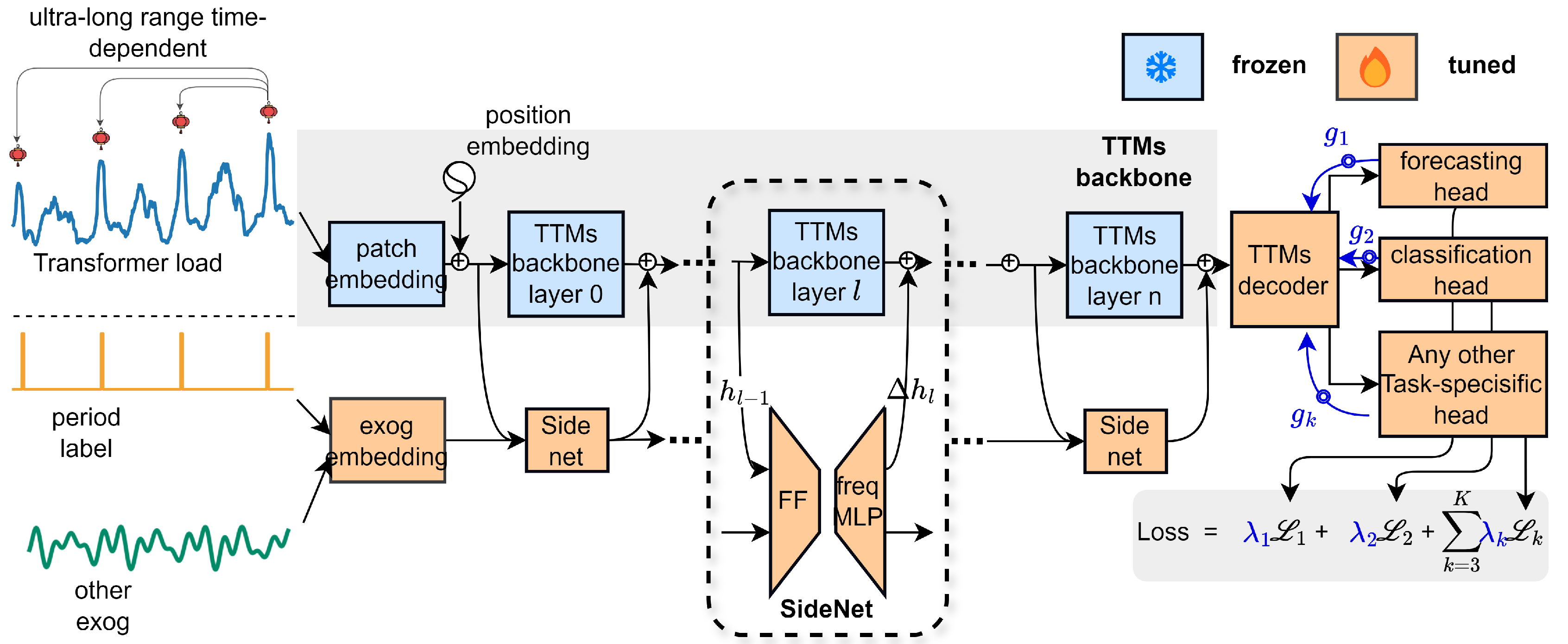
Figure 2.
Illustration of Load Forecasting in 2024 Spring Festival. (a) load surge observed in a transformer in southern China and the forecasting results of FreqMixer. (b) Comparison with traditional baseline. (d) Comparison with SOTA baseline
Figure 2.
Illustration of Load Forecasting in 2024 Spring Festival. (a) load surge observed in a transformer in southern China and the forecasting results of FreqMixer. (b) Comparison with traditional baseline. (d) Comparison with SOTA baseline
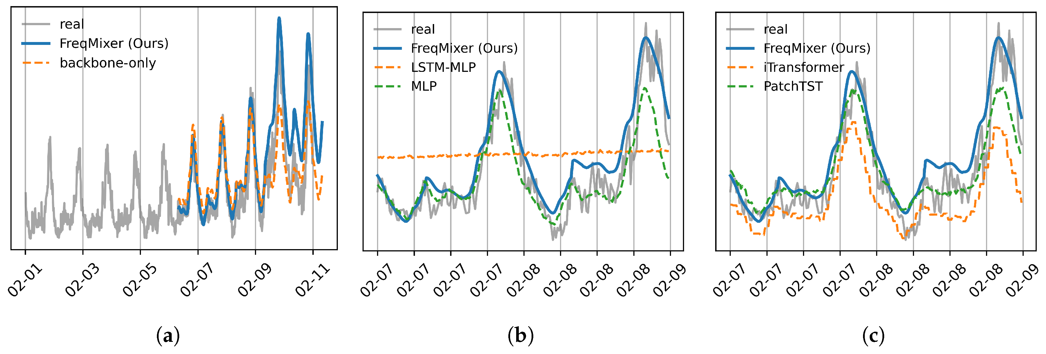

Table 1.
Load Forecasting Results.
| model | Leadtime/Metric | 1hour | 3hour | 6hour | 12hour | 1day | 2day | 3day | |
|---|---|---|---|---|---|---|---|---|---|
| SOTA TSF Models | TSMixerx | MAPE | 23.82 | 44.87 | 49.23 | 28.46 | 30.82 | 51.82 | 31.16 |
| Recall | 0.118 | 0.118 | 0.118 | 0.059 | 0.000 | 0.000 | 0.000 | ||
| Precision | 1.000 | 1.000 | 0.500 | 1.000 | 0.000 | 0.000 | 0.000 | ||
| iTransformer | MAPE | 23.9 | 24.68 | 26 | 27.44 | 30.22 | 34.75 | 37.37 | |
| Recall | 0.176 | 0.118 | 0.059 | 0.000 | 0.000 | 0.000 | 0.000 | ||
| Precision | 0.750 | 1.000 | 0.333 | 0.000 | 0.000 | 0.000 | 0.000 | ||
| TimeMixer | MAPE | 17.79 | 20.71 | 24.22 | 25.38 | 27.49 | 33.07 | 37.06 | |
| Recall | 0.294 | 0.176 | 0.118 | 0.118 | 0.118 | 0.000 | 0.000 | ||
| Precision | 1.000 | 1.000 | 1.000 | 1.000 | 1.000 | 0.000 | 0.000 | ||
| PatchTST | MAPE | 18.39 | 19.91 | 20.66 | 22.98 | 26.6 | 30.71 | 33.07 | |
| Recall | 0.882 | 0.588 | 0.412 | 0.235 | 0.294 | 0.118 | 0.000 | ||
| Precision | 0.441 | 0.455 | 0.333 | 0.235 | 0.139 | 0.047 | 0.000 | ||
| Baseline | lstm+mlp | MAPE | 26.09 | 26.33 | 26.74 | 27.48 | 28.38 | 29.50 | 29.86 |
| Recall | 0.000 | 0.000 | 0.000 | 0.000 | 0.000 | 0.000 | 0.000 | ||
| Precision | 0.000 | 0.000 | 0.000 | 0.000 | 0.000 | 0.000 | 0.000 | ||
| mlp | MAPE | 16.38 | 17.33 | 18.48 | 20.38 | 23.80 | 26.28 | 32.00 | |
| Recall | 0.700 | 0.600 | 0.650 | 0.450 | 0.500 | 0.250 | 0.158 | ||
| Precision | 0.519 | 0.500 | 0.481 | 0.310 | 0.385 | 0.208 | 0.125 | ||
| Foundation | FreqMixer | MAPE | 13.31 | 15.04 | 16.1 | 16.87 | 17.17 | 21.43 | 24.53 |
| Recall | 0.706 | 0.647 | 0.647 | 0.706 | 0.706 | 0.647 | 0.706 | ||
| Precision | 0.706 | 0.917 | 0.733 | 0.632 | 0.600 | 0.355 | 0.255 | ||
| TTms | MAPE | 23.27 | 27.85 | 28.32 | 28.56 | 29.72 | 42.76 | 53.54 | |
| Recall | 0.880 | 1.000 | 0.650 | 0.450 | 0.400 | 0.250 | 0.150 | ||
| Precision | 0.595 | 0.652 | 0.382 | 0.281 | 0.286 | 0.122 | 0.056 | ||
| Avg Imp. over best SOTA | MAPE ↓: -23.65%, Recall ↑: 87.42%, Precision ↑: 72.32% | ||||||||
Table 2.
Downstream Overload Prediction Task Results.
| Model | Accuracy | Precision | Recall | F1_score |
|---|---|---|---|---|
| FreqMixer | 0.9489 | 0.5652 | 0.619 | 0.5909 |
| Dlinear | 0.8324 | 0.1935 | 0.5714 | 0.2892 |
| mlp | 0.0653 | 0.0575 | 0.9524 | 0.1084 |
| lstm | 0.0597 | 0.0597 | 1 | 0.1126 |
| Avg Imp. | 14.00% | 2× | 8.33% | 1× |
Table 3.
Ablation Results on Network Structure.
| TASK | Single task | Multi task | |||||||||
|---|---|---|---|---|---|---|---|---|---|---|---|
| METHOD | full | head | Adapter | LoRA | SideNet | full | head | Adapter | LoRA | SideNet | |
| lead 1 day | MAE | 0.077 | 0.156 | 0.072 | 0.073 | 0.073 | 0.081 | 0.144 | 0.077 | 0.095 | 0.077 |
| MSE | 1.015 | 3.819 | 0.834 | 0.875 | 0.860 | 1.123 | 3.504 | 1.005 | 1.435 | 0.974 | |
| MAPE | 28.987 | 64.937 | 28.084 | 28.497 | 28.316 | 30.744 | 55.238 | 30.226 | 36.770 | 30.366 | |
| Accuracy | 0.241 | 0.000 | 0.433 | 0.406 | 0.433 | 0.176 | 0.000 | 0.400 | 0.161 | 0.429 | |
| Precision | 0.318 | 0.000 | 0.448 | 0.419 | 0.448 | 0.231 | 0.000 | 0.429 | 0.227 | 0.462 | |
| Recall | 0.500 | 0.000 | 0.929 | 0.929 | 0.929 | 0.429 | 0.000 | 0.857 | 0.357 | 0.857 | |
| F1 score | 0.389 | 0.000 | 0.605 | 0.578 | 0.605 | 0.300 | 0.000 | 0.571 | 0.278 | 0.600 | |
| lead 5 day | MAE | 0.219 | 0.179 | 0.205 | 0.215 | 0.214 | 0.259 | 0.155 | 0.206 | 0.265 | 0.215 |
| MSE | 6.240 | 4.893 | 5.394 | 5.920 | 5.736 | 8.546 | 4.036 | 5.228 | 8.675 | 5.598 | |
| MAPE | 93.913 | 75.774 | 84.639 | 87.907 | 87.522 | 109.766 | 59.757 | 86.595 | 114.597 | 90.281 | |
| Accuracy | 0.025 | 0.000 | 0.160 | 0.163 | 0.179 | 0.019 | 0.000 | 0.169 | 0.054 | 0.167 | |
| Precision | 0.030 | 0.000 | 0.165 | 0.167 | 0.182 | 0.021 | 0.000 | 0.180 | 0.061 | 0.174 | |
| Recall | 0.133 | 0.000 | 0.867 | 0.867 | 0.933 | 0.133 | 0.000 | 0.733 | 0.333 | 0.800 | |
| F1 score | 0.049 | 0.000 | 0.277 | 0.280 | 0.304 | 0.036 | 0.000 | 0.289 | 0.103 | 0.286 | |
| #Param | 0.8M | 0.3M | 1.6M | 1.6M | 1.3M | 1.7M | 0.3M | 1.6M | 1.6M | 2.9M | |
Table 4.
Downstream Overload Prediction Task Results.
| tune mode | d_model | MSE | MAE | #Param |
|---|---|---|---|---|
| SOTA Baseline PatchTST |
16 | 0.370 | 0.400 | 0.11M |
| full tune | / | 0.368 | 0.396 | 67.3M |
| FF | 16 | 0.373 | 0.401 | 0.27M |
| 32 | 0.369 | 0.400 | 0.53M | |
| 128 | 0.362 | 0.398 | 2.11M | |
| 512 | 0.399 | 0.421 | 8.41M | |
| FreqMLP | 2 | 0.362 | 0.399 | 0.05M |
| 4 | 0.354 | 0.394 | 0.09M | |
| 16 | 0.363 | 0.399 | 0.55M | |
| 32 | 0.369 | 0.402 | 1.08M | |
| FF+FreqMLP | 2 | 0.364 | 0.400 | 0.09M |
| 4 | 0.360 | 0.396 | 0.16M | |
| 8 | 0.359 | 0.396 | 0.29M | |
| 16 | 0.362 | 0.399 | 0.55M | |
| 32 | 0.362 | 0.401 | 1.08M |
Disclaimer/Publisher’s Note: The statements, opinions and data contained in all publications are solely those of the individual author(s) and contributor(s) and not of MDPI and/or the editor(s). MDPI and/or the editor(s) disclaim responsibility for any injury to people or property resulting from any ideas, methods, instructions or products referred to in the content. |
© 2024 by the authors. Licensee MDPI, Basel, Switzerland. This article is an open access article distributed under the terms and conditions of the Creative Commons Attribution (CC BY) license (http://creativecommons.org/licenses/by/4.0/).
Copyright: This open access article is published under a Creative Commons CC BY 4.0 license, which permit the free download, distribution, and reuse, provided that the author and preprint are cited in any reuse.


