
Submitted:
23 July 2025
Posted:
24 July 2025
You are already at the latest version
Abstract
Time series forecasting can be applied to various aspects of daily life, providing valuable insights to inform decision-making in areas such as stock market, electricity load, traffic flow and health-care, among others. Many previous studies have demonstrated the effectiveness of transformer-based models in long-term time series forecasting tasks, and the introduction of patch mechanisms can further enhance the predictive performance of Transformer-based models. However, most of the previous works have focused on reducing the computational resource overhead of patch-wise models, with little consideration given to the potential decrease in the model's ability to capture information from each time step within the patches. This often limits the further improvement of prediction accuracy in patch-wise models. To Address this issue, we propose a frequency compensation block, which incorporates frequency-domain data features into each patch before performing the time series forecasting task, to improve patch-wise model, called Frequency Compensation Patch-wise transFormer(FCP-Former). Experimental results demonstrate that the proposed method achieve better performance compared with the state-of-the-art methods in multivariate time series forecasting tasks.
Keywords:
time series forecasting
; frequency-domain
; transformer-based model
; patch-wise model
1. Introduction
Time series forecasting constitutes a statistical approach aimed at predicting future observations based on historical temporal data. This methodology has demonstrated extensive applicability across a broad spectrum of domains, including but not limited to meteorology[1,2], healthcare analytics[3,4], intelligent transportation systems[5,6] , electrical load forecasting[7,8], and financial risk assessment[9,10]. In recent years, recurrent neural network (RNN)-based architectures have been extensively employed for modeling time series data due to their capacity to learn temporal dependencies[11,12]. While these methods have yielded considerable empirical success [13,14], they are inherently constrained by several limitations, most notably the issues of vanishing and exploding gradients. These challenges significantly hinder the ability of RNNs to effectively model long-range dependencies within sequential data, thereby limiting their performance in scenarios requiring long-term forecasting accuracy.
After achieving great success in computer vision [15,16,17,18] and natural language processing [19,20,21,22], the transformer [23] model was introduced to time series forecasting to directly model the relationships between any two time steps in a sequence. Due to its powerful attention mechanism, transformer overcomes the gradient vanishing and gradient exploding problems that still trouble RNN and LSTM(Long Short-Term Memory)-type methods, making it a popular research topic in the field of time series forecasting.
Based on the token granularity fed into the attention mechanism in the time domain, existing Transformer-based research can be roughly divided into patch-wise models and point-wise models. A patch is a basic module formed by concatenating multiple temporally contiguous time-series data points. This enables the model to treat a patch as a token instead of treating each timestep as a token, significantly reducing the computational time. Based on different treatments of the variates, patch-wise models can be further divided into channel-independent strategy models and channel-dependent strategy models. Typical channel-independent strategy models include PatchTST [24], while channel-dependent strategy models include iTransformer[31] ,TimeXer[32] and Crossformer[33]. In contrast, point-wise models treat each time step and its corresponding variates as a token, which gives them a stronger ability to capture internal temporal variations. Typical point-wise models include FEDformer [25], Informer [26] and Autoformer [27]. However, due to their high computational complexity, it is challenging for these models to capture long-term dependencies between time series data.
For patch-wise models, patching the time series data can effectively reduce computational resource consumption. However, patch-wise methods embed each patch into a coarse token through a temporal linear projection, which leads to their inability to fully utilize the data within the patch, potentially compromising the accuracy of the final prediction.
Inspired by FEDformer [25] which utilizes frequency domain transformations, we recognize that some information in time series data may not be sufficiently captured in the time domain but can be effectively revealed in the frequency domain. For instance, periodic signals exhibit this characteristic.. As illustrated in Figure 1, in the time domain, data points are arranged in chronological order, with each data point representing the observation at a specific point in time. In the frequency domain, the data is decomposed into different frequency components, with each frequency component representing the extent of a particular periodicity in the signal. This representation facilitates the identification of periodicity and underlying trends in the data.
To address the loss caused by the model's inability to fully utilize the information of each piece of data within the patch, we propose a method that adds corresponding frequency domain information to the patched data, compensating for the information loss caused by patching, and propose an optimized PatchTST[24] called Frequency Compensation Patch-wise transFormer(FCP-Former). The main contributions of this paper are summarized as follows:
- We propose a frequency compensation block that adds corresponding frequency domain information to the patched data via frequency-domain representation learning, compensating for intra-patch information loss.
- We use the frequency compensation block to optimize PatchTST model, called FCP-Former, which better captures the periodic and trend changes in time series data.
- We conducted multivariate time series prediction experiments on eigth publicly available multivariate time series datasets. The proposed FCP-Former exhibits better comprehensive performance compared with the state-of-the-art methods.
2. Preliminaries and Related Work
2.1. Problem Definition
Time series data is a set of data arranged in chronological order. This type of data is typically collected at specific time points, and there is a temporal dependence between the data points. In time series forecasting, future events are predicted by utilizing these time-ordered data. The historical data can be defined as and the predicted data can be defined as . where D is the number of variables, L is the length of historical data, T is the length of predicted data. The concept of time series forecasting can be expressed as:
where is the predicted value, is the forecasting function, are the historical values and is the forecasting error.
2.2. Transformer-Based Time Series Forecaster
With the great success made in the field of natural language processing and computer vision, Transformer has gained the attention of researchers in the field of time series forecasting due to its powerful ability to capture long-term temporal dependencies and complex multivariate correlations. We briefly review several key variants below. Informer [26] addresses the high computational complexity of transformers in time series forecasting by proposing a sparse self-attention mechanism. FEDformer[25] enhances the transformer model's ability to capture global features of time series data by combining the transformer model with seasonal trend decomposition, while retaining key frequency information of the time series data through Fourier and wavelet transforms. PatchTST[24] improves the transformer’s ability to capture historical dependencies by using a channel-independent strategy to patch the time series data, reducing computational overhead while maintaining the ability to model long-range dependencies. Crossformer[33] enhances the transformer’s ability to handle multivariate time series forecasting tasks through dimension-segment-wise embedding and a two-stage attention mechanism. Npformer[28] introduces an innovative multi-scale segmented Fourier attention mechanism to more effectively capture dependencies. TimeXer[32] enhances the Transformer model's prediction accuracy by incorporating exogenous variables. iTransformer[31] applies the Transformer's attention mechanism along the variate dimension instead of the time dimension.
Most of these transformer-based models either focus on the attention mechanism, designing new attention mechanisms to reduce the complexity of the original attention mechanism, or process the time series data itself to better leverage the transformer, thus achieving better performance on forecasting, especially when the prediction length is long. However, these patch-wise transformer methods face a common problem — as shown in Figure 2, compared to point-wise methods, the patch-wise approach, where the model treats a patch as a single token, cannot fully utilize each piece of data, which results in information loss within the patch. TimeXer introduces exogenous variables to address this issue, however, the feature extracted from the time domain remains inherently limited. In contrast to TimeXer, we leverage the complementary nature of frequency-domain information to time-domain data. Our proposed frequency compensation block extracts features from the frequency domain, effectively overcoming the limitations of relying solely on time-domain feature extraction. This enables the model to better capture the periodic and trend characteristics of time series data.
2.3. Time Series Forecasting with Time-Frequency Analysis
The Fourier transform serves as a bridge for converting signals between the time and frequency domains, with the discrete Fourier transform (DFT) and discrete wavelet transform (DWT) commonly used tools for time-frequency analysis. Current mainstream time-frequency analysis methods can be categorized into two types. The first type involves transforming time-domain data into the corresponding Fourier spectrum, analyzing the Fourier spectrum to extract frequency-domain-based features, and then using inverse transformations to convert the data back to the time domain to obtain prediction results. Typical examples include FreTS [29], FITS [34], and SparseTSF [35]. In contrast, the second type simultaneously extracts features from both the time and frequency domains of time series data, with the extracted features then concatenated at the network output to produce the prediction result. A typical example is FEDformer [25]. The method proposed in this paper primarily addresses the issue of data loss within patches in patch-wise models. Since the first type of time-frequency analysis typically demands relatively low resource overhead, the proposed FCP-Former adopts this approach.
3. Method
As illustrated in Figure 3, our proposed FCP-Former includes the following components: patching, embedding, projection, encoder, and the frequency compensation block. Lu Han et al.[30] had demonstrated through extensive experiments that the prediction method using channel-independent strategies typically achieves better prediction results than the method using channel-dependent strategies. Therefore, FCP-Former, like PatchTST[24], adopts the channel-independent strategy. However, FCP-Former applies the frequency compensation block to process the patched data before encoding, adding corresponding frequency features to compensate for intra-patch information loss. While NPformer [31] designs a multi-scale segmented Fourier attention mechanism, iTransformer has demonstrated that the standard attention mechanism can also yield excellent results. Therefore, instead of modifying the attention mechanism, FCP-Former focuses on enriching the information within each patch.
3.1. Model Structure
FCP-Former consists of a patching module, a Frequency Compensation Block, and an encoder.
Patching: By adopting a channel-independent strategy, we divide the original time series data into D channels based on the data dimension D, and perform patching separately for each channel. The time series data in each channel can be represented as , where i represents the i-th channel among the D channels. Let the patch length be P, the patch step size be S, and the length of the time series data in the channel be L. The number of patches, N, can then be calculated as follows:
padding is applied at the end, meaning that when the last patch extends beyond the end of the series, the remaining positions within that patch are filled using the last observed value in the channel, ensuring that each patch has a consistent size. After patching, the original time series in each channel is transformed into a sequence of patches .
Frequency Compensation Block: The core function of the frequency compensation block is to perform representation learning on each patch in the frequency domain, using the features of the patch in the frequency domain as a supplement to the information that is overlooked for each time step within the patch. To achieve this, frequency compensation block first applies a Fast Fourier Transform (FFT) to the patch, converting the data within the patch to a frequency domain representation. Then, it performs representation learning in the frequency domain. Finally, an inverse Fourier transform is applied to convert the data back into a time-domain representation. The data in the processed patch represents a transformed version of the original data, enriched by the frequency domain representation learning, rather than the completely raw data. It also includes the frequency characteristics of the patch, which serves as a compensation for the information that is overlooked within the patch. We will analyze the frequency compensation block in detail in the next section.
Encoder: We use a vanilla Transformer encoder to map the patches processed by frequency compensation block into the latent representations. Each patch is embedded into a latent space of dimension D by using a learnable linear projection matrix and position encoding , which serves as the input to the encoder. Embedding process can be simply formulated as follows:
where is the frequency compensation block, is the result obtained after applying frequency compensation block to each patch, and is the embedded result used as the input of the encoder. Then the multi-head attention will transform them into query matrices , key matrices and value matrices . The attention output is ultimately obtained through scaled dot product. Attention process can be simply formulated as follows:
where and . After passing through the BatchNorm layers and feed forward network, the final predicted result can be obtained from a linear layer.
3.2. Analysis of Frequency Compensation Block
Discrete Fourier Transform (DFT):The core idea of the Fourier Transform is to decompose a signal in the time domain into a linear combination of a series of sine and cosine functions. Each sine and cosine function represents a specific frequency component of the signal. Thus, the Fourier transform can help us extract the frequency characteristics from time series data. For discrete signals, the Discrete Fourier Transform is used, and its formula is:
where is the complex value of the k-th frequency in the frequency domain; is the n-th sampling point of the time-domain signal; N is the length of the signal. Relatively the IDFT can be defined as:
The shows that for a signal of length N, the computational complexity of the DFT is . However, the Fast Fourier Transform (FFT) reduces the computational load by utilizing the symmetry and periodicity of the signal, breaking the computation into smaller parts, thus reducing its complexity to and significantly improving computational efficiency.
Representation Learning In The Frequency Domain: When performing Fast Fourier Transform on time series data, how to sample is an issue that must be addressed. Retaining all frequency components may inevitably be affected by noise, while preserving only a portion of the frequencies may risk missing some of the underlying trends in the data. FEDformer[28] demonstrates that real-world multivariate time series typically yield low-rank matrices after Fourier transform. This low-rank property implies that representing the time series by randomly selecting a fixed number of Fourier components is reasonable. Consequently, we adopt random sampling as our sampling method and set number of modes as M. After random sampling, the selected set of frequency indices is defined as Next, we define two weight tensors, and where represents the number of features, represents the number of patches, and represents the number of frequency components selected from the frequency domain after random sampling. These parameters represent the learnable weights of the network and are initialized with random values. The weights are used to perform weighted transformations on the input signal in the frequency domain. The input patch tensor is where B is the batch size, V is the number of features and PL is the length of each patch. We apply a Fast Fourier Transform (FFT) to the input tensor X along the PL dimension. A tensor is defined to store the frequency domain data after the Fourier transform. Finally,we use the Inverse Fourier transform (IFFT) to convert the processed frequency domain data back to the time domain. This process can be simply formulated as follows:
where is the input tensor, is the result obtained by applying the Fourier transform to , represents the learned complex weight for frequency i. is the frequency domain representation after the weighting operation, and thefinal output is .
4. Results
To verify the effectiveness and generality of FCP-Former, we conducted a comprehensive empirical study on eight real-world time-series long-term forecasting datasets, which are widely used in practical applications. To ensure a fair comparison with baseline methods that typically use shorter look-back windows, we set the input length of FCP-Former to 96 as those baselines. This configuration deliberately does not leverage the potential advantage of longer look-back windows afforded by the patching mechanism, focusing instead on the intrinsic capability of the proposed frequency compensation block. The results demonstrate that even under this constrained setting, FCP-Former achieves competitive performance in terms of MSE and MAE compared to existing state-of-the-art methods. Furthermore, we explore the performance of FCP-Former when utilizing longer look-back windows (336 and 512 input time steps), where it demonstrates superior predictive capabilities.
4.1 Experimental Setup
4.1.1. Datasets
We use eight real-world datasets widely used in time series forecasting research. We describe the datasets in detail as follows:
ETT (Electricity Transformer Temperature): consists of two years of data from two different electricity transformers. ETTh1 and ETTh2 are recorded every hour, and ETTm1 and ETTm2 are recorded every 15 minutes.
Traffic: contains data on hourly occupancy rates from 862 sensors of San Francisco Bay area freeways from January 2015 to December 2016.
Weather: provides 21 meteorological factors recorded every 10 minutes at the Weather Station of the Max Planck Biogeochemistry Institute in 2020.
Electricity: records the hourly electricity consumption of 321 customers.
ILI: describes the number of patients and influenza-like illness ratio at weekly intervals, sourced from the US Centers for Disease Control and Prevention between 2002 and 2021.
The statistics of those datasets are summarized in Table 1.
4.1.2. Baselines and Experimental Settings
We choose the SOTA transformer-based model as the baseline, including PatchTST[24], iTransformer[31], TimeXer[32], FEDformer[25], Crossformer[33] and Autoformer[27]. All of the models follow the same experimental setup with prediction length for ILI dataset and for other datasets. To verify the effectiveness and generality of proposed method, we set the input length of the proposed model to 96. This input length is typically used by point-wise methods. The statistics of those baselines are summarized in Table 2.
4.1.3. Metrics
we choose the mean square error(MSE) and mean absolute error(MAE) as evaluation metrics, which can be defined as:
where N is the prediction length, is the ground truth at timestamp within the forecast horizon and is the predicted value at timestamp . A lower MSE or MAE indicates better forecasting performance.
4.1.4. Implementation Details
Our model was implemented with PyTorch2.4.0 and trained on an NVIDIA GeForce RTX4090 GPU. We used the Adam optimizer and set the learning rate to 1e-4 to train our model. For small datasets, such as the ETT dataset, we set the batch size to 128. For larger datasets like traffic, due to memory resource limitations, we adjust the batch size between 8 and 32. For all datasets, we set the maximum number of training epochs to 50. To preventoverfitting and reduce training time, we set the dropout rate to 0.05 and use an early stopping mechanism with a patience of 3 to halt training when the validation loss showed no significant decrease. The patch length, denoted as P, was set to 16. The hyperparameter frequency modes, denoted as M, were set to 16.
4.2. Experimental Results
For multivariate forecasting, FCP-Former outperforms other methods on all eight benchmark datasets, as shown in Table 3. The experimental results indicate that FCP-Former significantly outperforms other baseline methods in prediction performance for multivariate long-term time series forecasting tasks. FCP-Former achieves a total of 48 optimal values and 17 suboptimal values, especially on the ETT and electricity datasets. Although FCP-Former does not achieve the best performance on all datasets, it consistently attains near-optimal results. This demonstrates. that FCP-Former exhibits significant advantages in long-term forecasting. It is worth noting that, compared to baseline methods, FCP-Former often exhibits a smaller MAE when the MSE values are similar. This indicates smaller average deviations between predictions and ground truth, reflecting higher overall prediction accuracy. In practical application scenarios, such as stock price forecasting, supply chain management, and healthcare, where a lower MAE is more critical, our model demonstrates a distinct advantage.
4.3. Model Analysis
We will analyze FCP-Former through ablation studies, hyperparameter sensitivity experiments and experiments with different input lengths.
4.3.1. Ablation Studies
In this section, we conduct an ablation study on the model to demonstrate the effectiveness of our frequency compensation block. The following component is ablated:
- w/o FCB: Removing the frequency compensation block before encoding.
We compare the performance of the FCP-Former ablation version and the results of the full FCP-Former model in Table 4. From the results of the ablation experiment, it is evident that the application of the frequency compensation block leads to improved prediction performance.
4.3.2. Hyperparameter Sensitivity Experiments
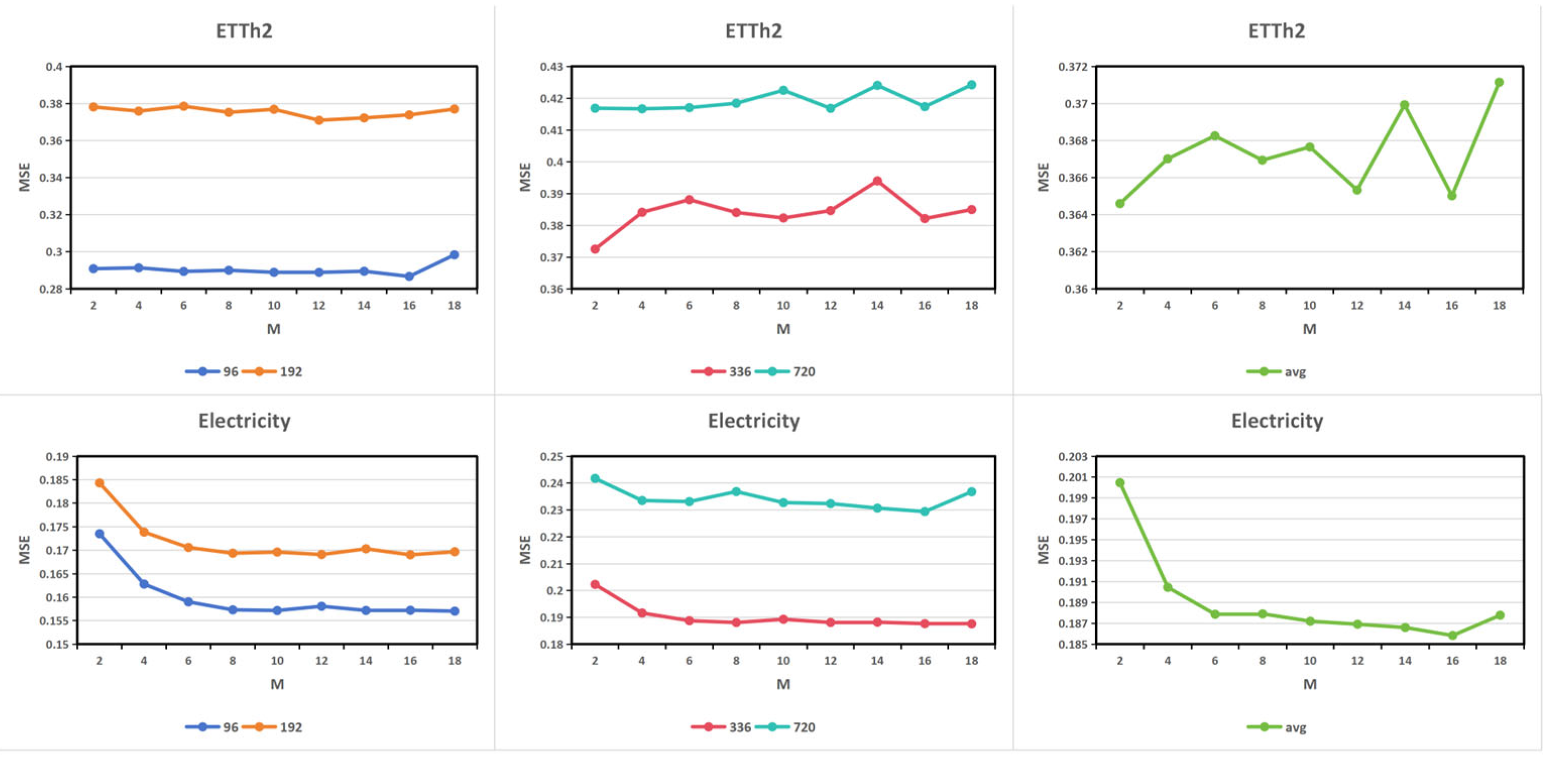
In frequency compensation block, we employed a crucial hyperparameter: the number of modes in the frequency domain M. This hyperparameter determines how many frequency components are selected from the frequency domain for the model to learn from. Its value directly impacts both the model's frequency domain representation capability and computational complexity. Theoretically, a larger number of modes implies more frequency patterns are used, resulting in higher frequency domain resolution and finer data variations being captured, but at the cost of increased computational load and a higher risk of overfitting. On the other hand, a smaller number of modes compresses the frequency domain information, with the model focusing only on the main low-frequency components. This makes the model lighter and faster, but may lead to the loss of high-frequency information, decreasing representational capacity while potentially improving generalization performance. In our experiments, we evaluate the number of modes in the frequency domain M from the set {2,4,6,8,10,12,14,16,18}. The results are shown in Figure 4. This figure corroborates the aforementioned theoretical analysis. When the value of M is low, the model learns fewer frequency patterns, resulting in relatively lower prediction accuracy. As M increases, the MSE gradually decreases and plateaus. When M reaches 16, the model achieves its optimal performance for this hyperparameter on both the ETTh2 and Electricity datasets. However, as M continues to increase, the model's prediction performance deteriorates due to overfitting, leading to a rise in MSE. This trend of performance deterioration due to overfitting is more pronounced on the Electricity dataset. Considering both computational costs and prediction performance, we recommend setting the value of M to 16.
Figure 4.
The MSE results with different number of selected modes in the ETTh1(upper row) and Electricity(lower row) datasets.
Figure 4.
The MSE results with different number of selected modes in the ETTh1(upper row) and Electricity(lower row) datasets.
4.3.3. Experiments with Different Input Lengths
In time series forecasting tasks, the input length determines the amount of historical information available to the model. A longer look-back window allows the model to capture a broader range of past observations, thereby expanding its perceptual scope. For a model with strong long-term time dependency modeling corresponding to models referred to as FCP-Former-336 and FCP-Former-512. Since a longer look-back window inevitably leads to increased memory overhead, we dynamically adjusted the batch size to balance memory consumption. Due to the limited size of the ILI dataset, with only 966 data points, increasing the input length leads to a reduction in the training set size. For FCP-Former-512, using the dataset split as shown in Table I, the training set consists of only 8 data points, making training impossible. Similarly, for FCP-Former-336, the training set contains only 184 data points, which is insufficient for adequate model training. Therefore, we did not conduct experiments on the ILI dataset. For the remaining datasets, the comparative results of FCP-Former, FCP-Former-336, and FCP-Former-512 are presented in Table 5. Based on the work of Wang et al[36]., it is evident that due to the presence of repeated short-term patterns in the data, and the difficulty of Transformer models in effectively capturing and modeling these short-term patterns, the performance of Transformer-based models often deteriorates as the input length increases. This phenomenon helps explain why, in a few specific cases, the performance of FCP-Former-336 marginally outperformed that of FCP-Former-512. However, overall, the performance of FCP-Former-512 surpasses that of both FCP-Former-336 and FCP-Former, particularly when the prediction length is higher, where its advantages become even more pronounced. The overall superior performance of FCP-Former-512, particularly for longer prediction horizons, suggests that FCP-Former excels in capturing long-term temporal dependencies and in deeply extracting meaningful information from historical data.
4.4. Multivariate Showcases
As shown in Figure 5, we also compare the prediction results of FCP-Former with those of recently established state-of-the-art models (PatchTST, TimeXer and iTransformer) on the test sets of multiple datasets (ETTm1, Weather, and Electricity). Our model demonstrates predictions that are closest to the ground truth values, providing a direct visual manifestation of its superior MAE performance reported in Table 3. Furthermore, due to its enhanced ability to capture the trend of time series data, FCP-Former exhibits a significant advantage in predicting the overall trend, as evidenced by the close alignment between its predicted trends and the actual trends.
5. Conclusions
In this work, we have proposed a frequency compensation block to optimize the patch-wise transformer-based model in long time series prediction tasks. The frequency compensation block enables the model to perform representation learning of time series data in the frequency domain, enriching the information within each patch of the patch-wise model. This allows the model to more effectively capture the periodic and trend components within the data when performing time series forecasting tasks, and uncovers key information hidden in the raw data. Experimental results on several real-world time series datasets demonstrate that FCP-Former achieves state-of-the-art performance in long-sequence prediction tasks, with predictions that are closer to the true values, better meeting the requirements of practical application scenarios. In future research, we aim to investigate the model's performance on datasets with more chaotic periodic and trend components, to further mitigate the impact of noise on the accuracy of model predictions.
Author Contributions
Conceptualization, M.L. and M.Y.; methodology, M.L. and M.Y .; software, M.Y.; validation, M.Y., S.C. and H.L.; investigation, G.X.; data curation,S.L.; writing—original draft preparation, M.Y.; writing—review and editing, all authors.; visualization, M.Y.; All authors have read and agreed to the published version of the manuscript.
Funding
Please add: This work was funded by the Deep Earth Probe and Mineral Resources Exploration-National Science and Technology Major Project (2024ZD1003905).
Institutional Review Board Statement
Not applicable.
Informed Consent Statement
Not applicable.
Data Availability Statement:
ETT datasets: HTTPS://GITHUB.COM/ZHOUHAOYI/ETDATASET, Traffic datasets: HTTP://PEMS.DOT.CA.GOV, Weather datasets:https://www.bgc-jena.mpg.de/wetter/,Electricity datasets: https://archive.ics.uci.edu/ml/datasets/ElectricityLoadDiagrams20112014, ILI datasets: https://gis.cdc.gov/grasp/fluview/fluportaldashboard.html. Further inquiries can be directed to the corresponding author
Conflicts of Interest
The authors declare no conflicts of interest.
Abbreviations
The following abbreviations are used in this manuscript:
| RNN | recurrent neural network |
| LSTM | Long Short-Term Memory |
| DFT | Discrete Fourier Transform |
| FFT | fast Fourier transform |
References
- K. Stephan, G. Jisha, and IEEE, "Enhanced Weather Prediction with Feature Engineered, Time Series Cross Validated Ridge Regression Model," in 2024 CONTROL INSTRUMENTATION SYSTEM CONFERENCE, CISCON 2024, 2024-01-01 2024. [CrossRef]
- S. Sharma, K. Bhatt, R. Chabra, and N. Aneja, "A Comparative Performance Model of Machine Learning Classifiers on Time Series Prediction for Weather Forecasting," in ADVANCES IN INFORMATION COMMUNICATION TECHNOLOGY AND COMPUTING, AICTC 2021, 2022-01-01 2022, vol. 392, pp. 577-587. [CrossRef]
- P. Melin, J. Monica, D. Sanchez, and O. Castillo, "Multiple Ensemble Neural Network Models with Fuzzy Response Aggregation for Predicting COVID-19 Time Series: The Case of Mexico," HEALTHCARE, vol. 8, no. 2, 2020-06-01 2020, Art no. 181. [CrossRef]
- R. Sharma, M. Kumar, S. Maheshwari, and K. Ray, "EVDHM-ARIMA-Based Time Series Forecasting Model and Its Application for COVID-19 Cases," IEEE TRANSACTIONS ON INSTRUMENTATION AND MEASUREMENT, vol. 70, 2021-01-01 2021, Art no. 6502210. [CrossRef]
- Y. Fang, Y. Qin, H. Luo, F. Zhao, and K. Zheng, "STWave+: A Multi-Scale Efficient Spectral Graph Attention Network With Long-Term Trends for Disentangled Traffic Flow Forecasting," IEEE TRANSACTIONS ON KNOWLEDGE AND DATA ENGINEERING, vol. 36, no. 6, pp. 2671-2685, 2024-06-01 2024. [CrossRef]
- K. Elmazi, D. Elmazi, E. Musta, F. Mehmeti, and F. Hidri, "An Intelligent Transportation Systems-Based Machine Learning-Enhanced Traffic Prediction Model using Time Series Analysis and Regression Techniques," in 2024 INTERNATIONAL CONFERENCE ON INNOVATIONS IN INTELLIGENT SYSTEMS AND APPLICATIONS, INISTA, 2024-01-01 2024. [CrossRef]
- H. Iftikhar, S. Gonzales, J. Zywiolek, and J. López-Gonzales, "Electricity Demand Forecasting Using a Novel Time Series Ensemble Technique," IEEE ACCESS, vol. 12, pp. 88963-88975, 2024-01-01 2024. [CrossRef]
- S. Gonzales, H. Iftikhar, and J. López-Gonzales, "Analysis and forecasting of electricity prices using an improved time series ensemble approach: an application to the Peruvian electricity market," AIMS MATHEMATICS, vol. 9, no. 8, pp. 21952-21971, 2024-01-01 2024. [CrossRef]
- Y. Hsu, Y. Tsai, and C. Li, "FinGAT: Financial Graph Attention Networks for Recommending Top-$K$K Profitable Stocks," IEEE TRANSACTIONS ON KNOWLEDGE AND DATA ENGINEERING, vol. 35, no. 1, pp. 469-481, 2023-01-01 2023. [CrossRef]
- S. Pal and S. Kar, "Fuzzy transfer learning in time series forecasting for stock market prices," SOFT COMPUTING, vol. 26, no. 14, pp. 6941-6952, 2022-01-24 2022. [CrossRef]
- W. Zhou, C. Zhu, and J. Ma, "Single-layer folded RNN for time series prediction and classification under a non-Von Neumann architecture," DIGITAL SIGNAL PROCESSING, vol. 147, 2024-02-13 2024, Art no. 104415. [CrossRef]
- R. Murata, F. Okubo, T. Minematsu, Y. Taniguchi, and A. Shimada, "Recurrent Neural Network-FitNets: Improving Early Prediction of Student Performanceby Time-Series Knowledge Distillation," JOURNAL OF EDUCATIONAL COMPUTING RESEARCH, vol. 61, no. 3, pp. 639-670, 2022-10-26 2023. [CrossRef]
- C. Zhang, J. Liu, and S. Zhang, "Online Purchase Behavior Prediction Model Based on Recurrent Neural Network and Naive Bayes," JOURNAL OF THEORETICAL AND APPLIED ELECTRONIC COMMERCE RESEARCH, vol. 19, no. 4, pp. 3461-3476, 2024-12-01 2024. [CrossRef]
- M. Monti, J. Fiorentino, E. Milanetti, G. Gosti, and G. Tartaglia, "Prediction of Time Series Gene Expression and Structural Analysis of Gene Regulatory Networks Using Recurrent Neural Networks," ENTROPY, vol. 24, no. 2, 2022-02-01 2022, Art no. 141. [CrossRef]
- S. Elmi, B. Morris, and IEEE, "Res-ViT: Residual Vision Transformers for Image Recognition Tasks," in 2023 IEEE 35TH INTERNATIONAL CONFERENCE ON TOOLS WITH ARTIFICIAL INTELLIGENCE, ICTAI, 2023-01-01 2023, pp. 309-316 [Online]. Available: https://ieeexplore.ieee.org/stampPDF/getPDF.jsp?tp=&arnumber=10356246&ref=. [CrossRef]
- L. Meng et al., "AdaViT: Adaptive Vision Transformers for Efficient Image Recognition," in 2022 IEEE/CVF CONFERENCE ON COMPUTER VISION AND PATTERN RECOGNITION (CVPR), 2022-01-01 2022, pp. 12299-12308. [Online]. Available: https://ieeexplore.ieee.org/stampPDF/getPDF.jsp?tp=&arnumber=9879366&ref=. [CrossRef]
- S. Nag, G. Datta, S. Kundu, N. Chandrachoodan, P. Beerel, and IEEE, "ViTA: A Vision Transformer Inference Accelerator for Edge Applications," in 2023 IEEE INTERNATIONAL SYMPOSIUM ON CIRCUITS AND SYSTEMS, ISCAS, 2023-01-01 2023. [Online]. Available: https://ieeexplore.ieee.org/stampPDF/getPDF.jsp?tp=&arnumber=10181988&ref=. [CrossRef]
- Z. Yang et al., "LAVT: Language-Aware Vision Transformer for Referring Image Segmentation," in 2022 IEEE/CVF CONFERENCE ON COMPUTER VISION AND PATTERN RECOGNITION (CVPR 2022), 2022-01-01 2022, pp. 18134-18144. [Online]. Available: https://ieeexplore.ieee.org/stampPDF/getPDF.jsp?tp=&arnumber=9880242&ref=. [CrossRef]
- H. Lin, L. Yang, and P. Wang, "W-core Transformer Model for Chinese Word Segmentation," in TRENDS AND APPLICATIONS IN INFORMATION SYSTEMS AND TECHNOLOGIES, VOL 1, 2021-01-01 2021, vol. 1365, pp. 270-280. [Online]. Available: https://link.springer.com/content/pdf/10.1007/978-3-030-72657-7_26.pdf. [CrossRef]
- M. Nguyen, V. Lai, A. Ben Veyseh, T. Nguyen, and A. C. LINGUIST, "Trankit: A Light-Weight Transformer-based Toolkit for Multilingual Natural Language Processing," in EACL 2021: THE 16TH CONFERENCE OF THE EUROPEAN CHAPTER OF THE ASSOCIATION FOR COMPUTATIONAL LINGUISTICS: PROCEEDINGS OF THE SYSTEM DEMONSTRATIONS, 2021-01-01 2021, pp. 80-90.
- S. Sarkar, M. Babar, M. Hassan, M. Hasan, S. Santu, and A. C. MACHINERY, "Processing Natural Language on Embedded Devices: How Well Do Transformer Models Perform?," in PROCEEDINGS OF THE 15TH ACM/SPEC INTERNATIONAL CONFERENCE ON PERFORMANCE ENGINEERING, ICPE 2024, 2024-01-01 2024, pp. 211-222. [CrossRef]
- L. Molinaro, R. Tatano, E. Busto, A. Fiandrotti, V. Basile, and V. Patti, "DelBERTo: A Deep Lightweight Transformer for Sentiment Analysis," in AIXIA 2022 - ADVANCES IN ARTIFICIAL INTELLIGENCE, 2023-01-01 2023, vol. 13796, pp. 443-456. [Online]. Available: https://link.springer.com/content/pdf/10.1007/978-3-031-27181-6_31.pdf. [CrossRef]
- A. Vaswani et al., "Attention Is All You Need," in ADVANCES IN NEURAL INFORMATION PROCESSING SYSTEMS 30 (NIPS 2017), 2017-01-01 2017, vol. 30, WOS.ISTP ed.
- Y. Nie, N. Nguyen, P. Sinthong, and J. Kalagnanam, "A Time Series is Worth 64 Words: Long-term Forecasting with Transformers," Arxiv, 2023-03-05 2023. arXiv:2211.14730.
- T. Zhou, Z. Ma, Q. Wen, X. Wang, L. Sun, and R. Jin, "FEDformer: Frequency Enhanced Decomposed Transformer for Long-term Series Forecasting," in 39th International Conference on Machine Learning (ICML), Baltimore, MD, 2022 Jul 17-23 2022, in Proceedings of Machine Learning Research, 2022. [Online]. Available: <Go to ISI>://WOS:000900130208024. [Online]. Available: <Go to ISI>://WOS:000900130208024.
- H. Zhou et al., "Informer: Beyond Efficient Transformer for Long Sequence Time-Series Forecasting," Proceedings of the AAAI Conference on Artificial Intelligence, vol. 35, no. 12, pp. 11106-11115, 2021. [CrossRef]
- H. Wu, J. Xu, J. Wang, and M. Long, "Autoformer: Decomposition Transformers with Auto-Correlation for Long-Term Series Forecasting," in ADVANCES IN NEURAL INFORMATION PROCESSING SYSTEMS 34 (NEURIPS 2021), 2021-01-01 2021, vol. 34.
- H. Tong, L. Kong, J. Liu, S. Gao, Y. Xu, and Y. Chen, "Segmented Frequency-Domain Correlation Prediction Model for Long-Term Time Series Forecasting Using Transformer," IET SOFTWARE, vol. 2024, 2024-07-08 2024, Art no. 2920167. [CrossRef]
- K. Yi et al., "Frequency-domain MLPs are More Effective Learners in Time Series Forecasting," in ADVANCES IN NEURAL INFORMATION PROCESSING SYSTEMS 36 (NEURIPS 2023), 2023-01-01 2023.
- .Han, H. Ye, and D. Zhan, "The Capacity and Robustness Trade-Off: Revisiting the Channel Independent Strategy for Multivariate Time Series Forecasting," IEEE TRANSACTIONS ON KNOWLEDGE AND DATA ENGINEERING, vol. 36, no. 11, pp. 7129-7142, 2024-11-01 2024. [CrossRef]
- Y. Liu, T. Hu, H. Zhang, H. Wu, S. Wang, L. Ma, and M. Long, “itransformer: Inverted transformers are effective for time series forecasting,”in International Conference on Learning Representations, 2024.
- Wang Y , Wu H , Dong J ,et al.TimeXer: Empowering Transformers for Time Series Forecasting with Exogenous Variables[J]. 2024.
- Yunhao Zhang and Junchi Yan. Crossformer: Transformer utilizing cross-dimension dependency for multivariate time series forecasting. In ICLR, 2022.
- Z. Xu, A. Zeng, and Q. Xu, “FITS: Modeling time series with $10k$parameters,” in International Conference on Learning Representations, 2024.
- S. Lin, W. Lin, W. Wu, H. Chen, and J. Yang, “Sparsetsf: Modeling long-term time series forecasting with 1k parameters,” arXiv preprint arXiv:2405.00946, 2024.
- H. Wang, J. Peng, F. Huang, J. Wang, J. Chen, and Y. Xiao, “MICN: Multiscale local and global context modeling for long-term series forecasting,”in Proc. 11th Int. Conf. Learn. Representations, 2023, pp. 1–11.
Figure 1.
(a): Time-domain plots of a sine wave with a frequency of 5; (b) frequency-domain(right) plots of a sine wave with a frequency of 5.
Figure 1.
(a): Time-domain plots of a sine wave with a frequency of 5; (b) frequency-domain(right) plots of a sine wave with a frequency of 5.
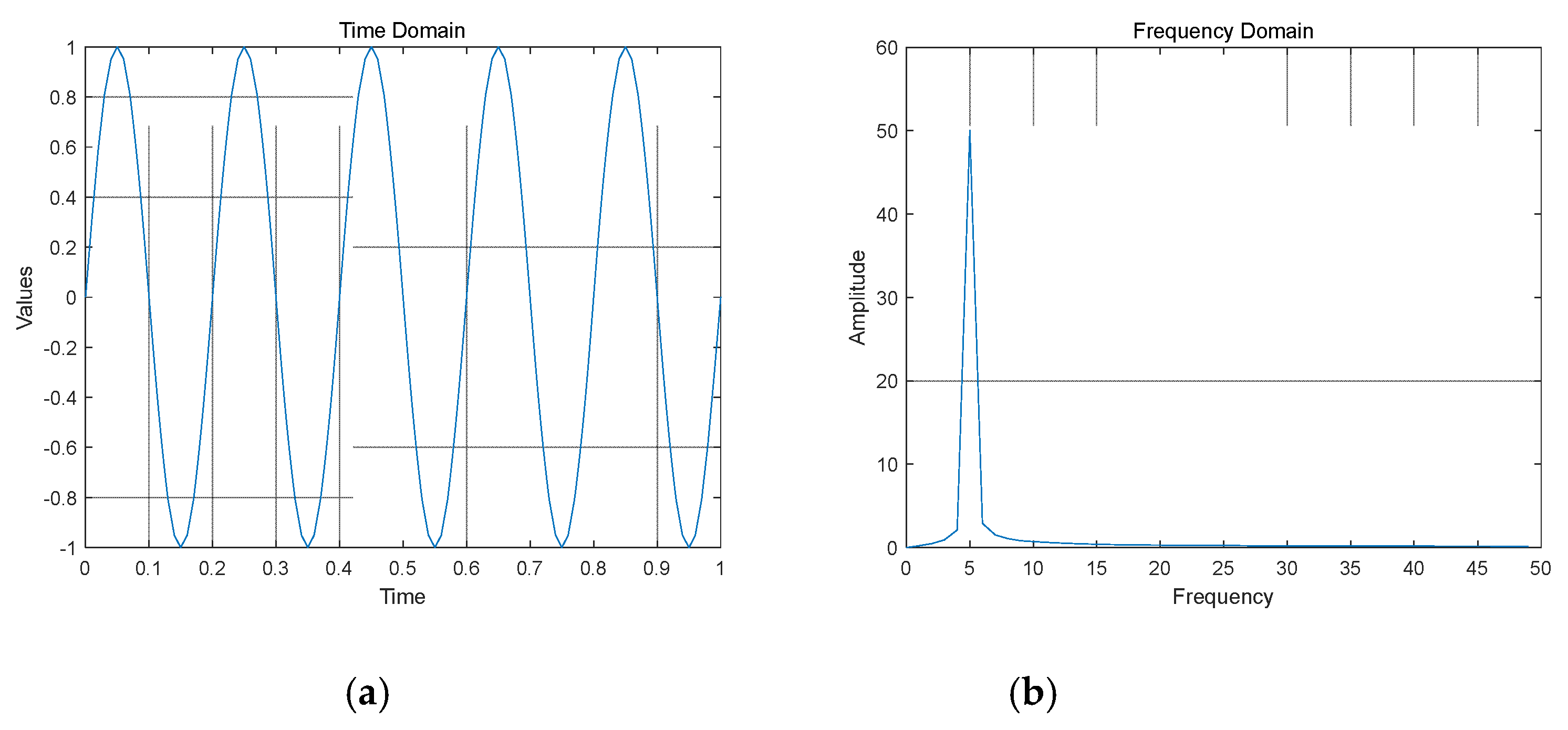
Figure 2.
Some data from the ETTh1 dataset. The red dashed lines represent tokens from point-wise models, the blue rectangular areas represent tokens from patch-wise models using channel-dependent strategies, and the green rectangular areas represent tokens from patch-wise models using channel-independent strategies.
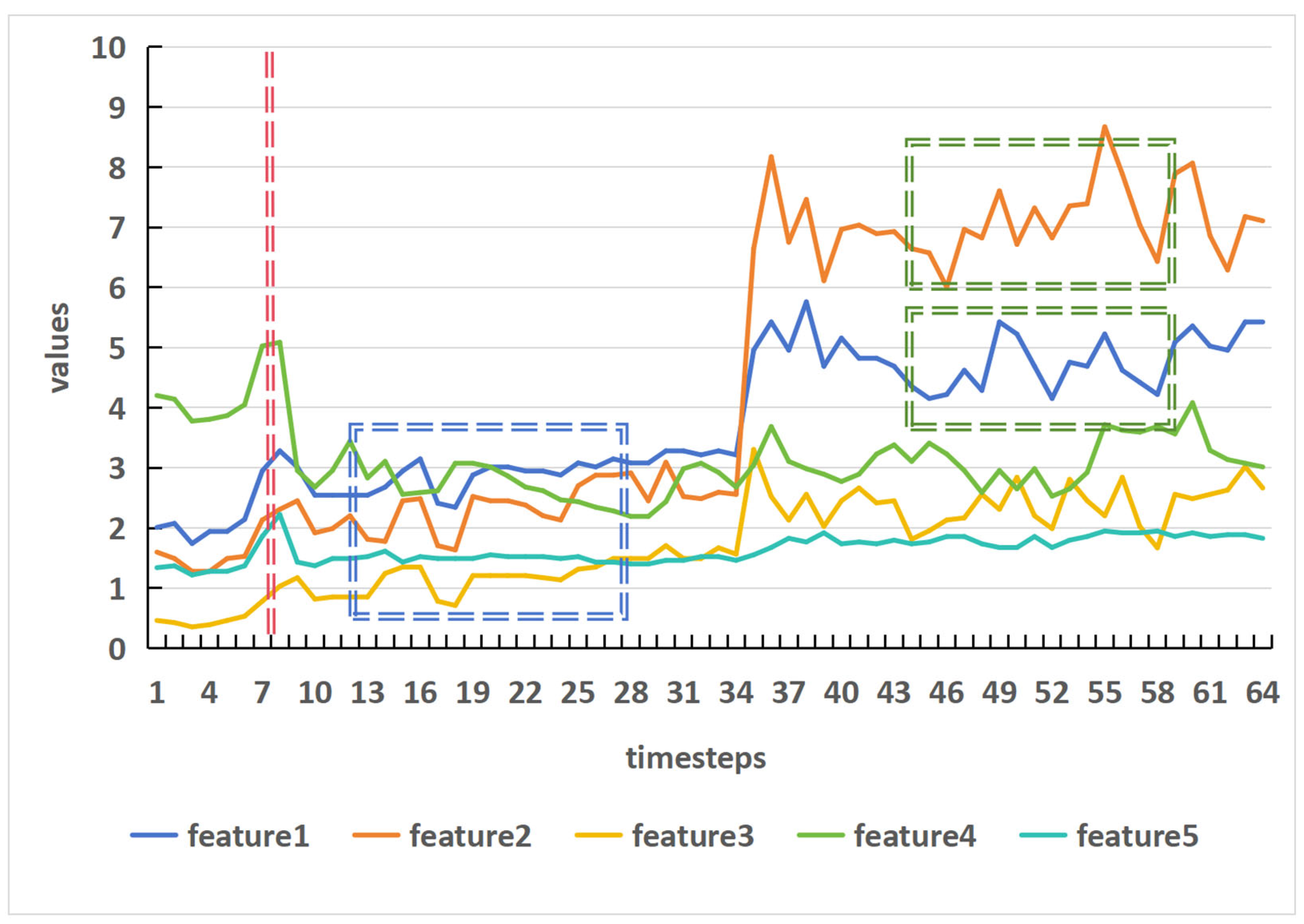
Figure 3.
FCP-Former uses a channel-independent strategy and employs a frequency compensation block to perform representation learning in the frequency domain for each patch. The learned data is then converted back to the time domain via an inverse Fourier transform for embedding operations. The vanilla transformer encoder and linear layers are used to produce the prediction results.
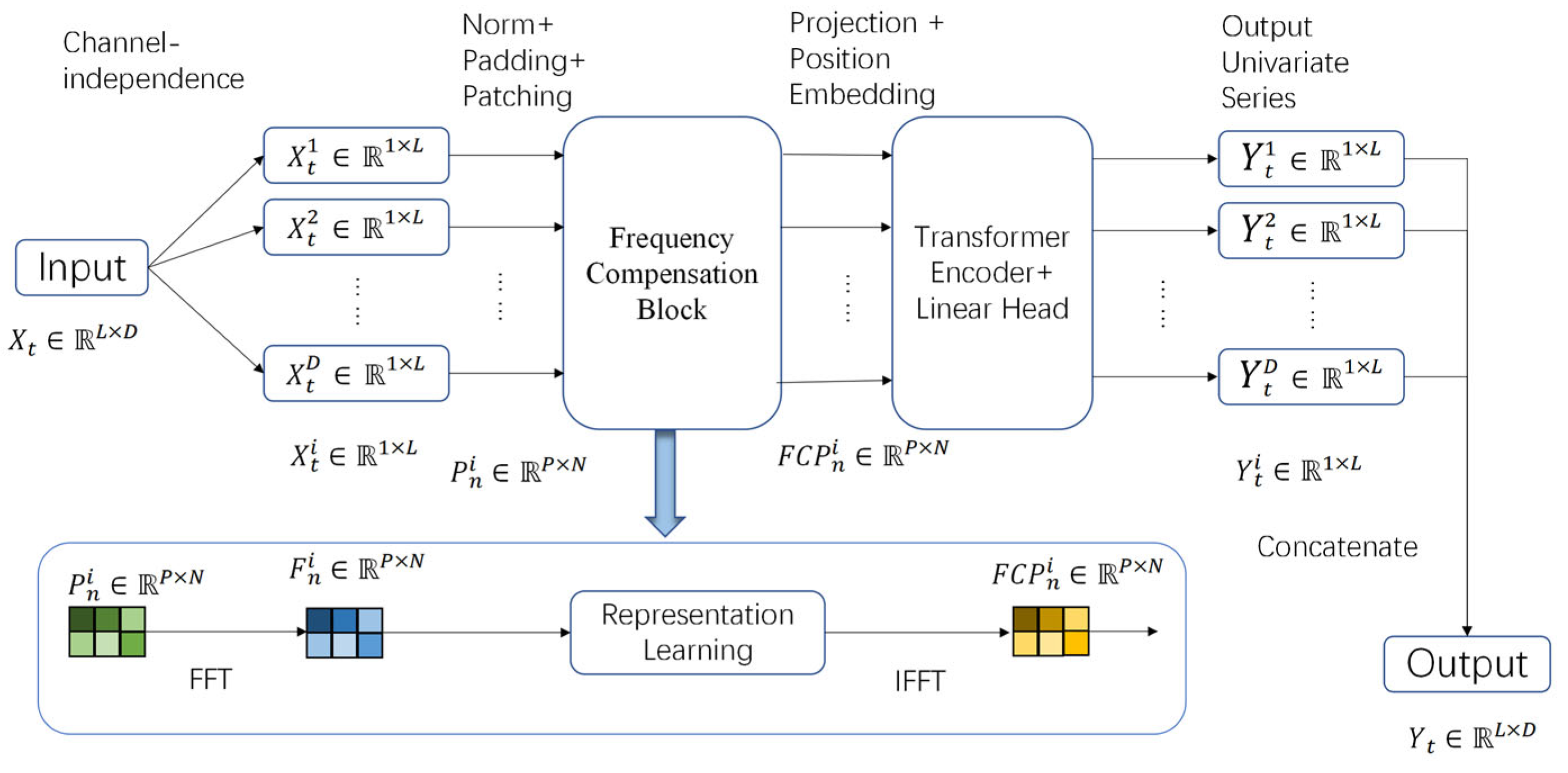
Figure 5.
visualization results of forecasting sequence randomly selected from ETTm1 (upper row), Weather (middle row) and Electricity (lower row). (a): The visualization of the prediction results of FCP-Former; (b): The visualization of the prediction results of PatchTST; (c): The visualization of the prediction results of TimeXer; (d): The visualization of the prediction results of iTransformer.
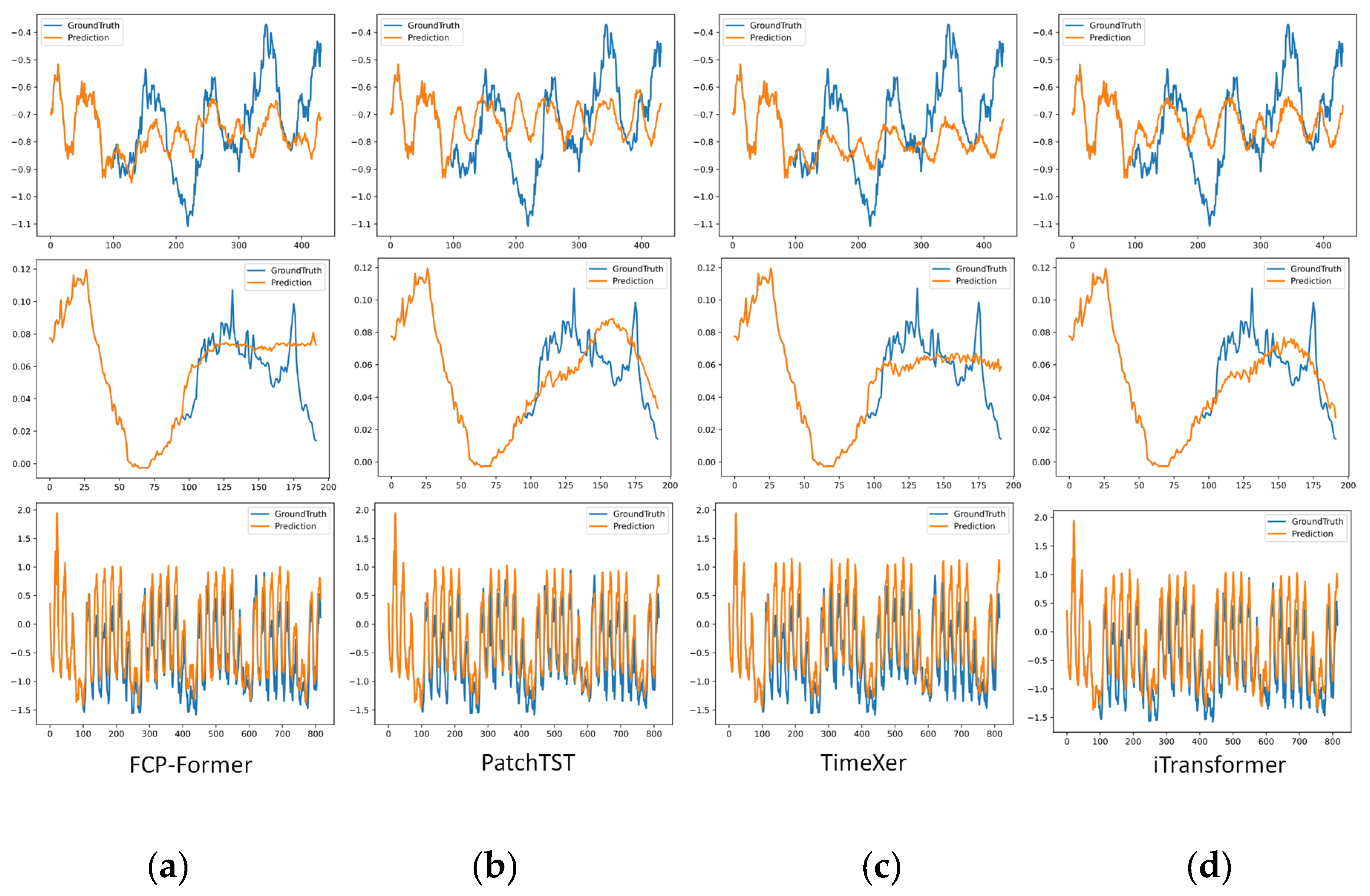

Table 1.
Details of datasets.
| Datasets | ETTh | ETTm | Traffic | Weather | Electricity | ILI |
| Timesteps | 17420 | 69680 | 17544 | 52696 | 26304 | 966 |
| Features | 7 | 7 | 862 | 21 | 321 | 7 |
| Partitions (train/val/test) |
12/4/4 | 12/4/4 | 7/1/2 | 7/1/2 | 7/1/2 | 6/2/2 |
Table 2.
Details of baselines.
| Models | Type | Sources | Strategy |
| PatchTST | Patch-wise | ICLR2023 | CI |
| iTransformer | Patch-wise | ICLR2024 | CD |
| TimeXer | Patch-wise | NeurIPS2024 | CD |
| FEDformer | Point-wise | ICML2022 | CD |
| Crossformer | Patch-wise | ICLR2023 | CD |
| Autoformer | Point-wise | NeurIPS2021 | CD |
Table 3.
Multivariate long-term forecasting results.
| Methods | FCP-Former | PatchTST | iTransformer | TimeXer | FEDformer | Crossformer | Autoformer | ||||||||
| Metric | MSE | MAE | MSE | MAE | MSE | MAE | MSE | MAE | MSE | MAE | MSE | MAE | MSE | MAE | |
| ETTh1 | 96 | 0.378 | 0.395 | 0.378 | 0.395 | 0.385 | 0.404 | 0.386 | 0.399 | 0.388 | 0.425 | 0.384 | 0.408 | 0.447 | 0.451 |
| 192 | 0.426 | 0.421 | 0.443 | 0.435 | 0.441 | 0.438 | 0.438 | 0.432 | 0.437 | 0.450 | 0.433 | 0.435 | 0.486 | 0.475 | |
| 336 | 0.472 | 0.445 | 0.493 | 0.461 | 0.479 | 0.456 | 0.483 | 0.455 | 0.482 | 0.476 | 0.677 | 0.628 | 0.505 | 0.490 | |
| 720 | 0.471 | 0.460 | 0.527 | 0.499 | 0.489 | 0.482 | 0.491 | 0.476 | 0.502 | 0.498 | 0.670 | 0.616 | 0.517 | 0.519 | |
| avg | 0.437 | 0.430 | 0.460 | 0.447 | 0.449 | 0.445 | 0.449 | 0.440 | 0.452 | 0.462 | 0.541 | 0.522 | 0.489 | 0.484 | |
| ETTh2 | 96 | 0.287 | 0.339 | 0.292 | 0.343 | 0.297 | 0.347 | 0.289 | 0.342 | 0.339 | 0.383 | 0.678 | 0.634 | 0.344 | 0.385 |
| 192 | 0.374 | 0.394 | 0.373 | 0.399 | 0.378 | 0.398 | 0.371 | 0.394 | 0.414 | 0.427 | 1.141 | 0.745 | 0.422 | 0.433 | |
| 336 | 0.382 | 0.412 | 0.390 | 0.416 | 0.426 | 0.433 | 0.419 | 0.430 | 0.453 | 0.464 | 1.200 | 0.764 | 0.455 | 0.464 | |
| 720 | 0.417 | 0.437 | 0.422 | 0.443 | 0.430 | 0.448 | 0.416 | 0.438 | 0.480 | 0.487 | 1.384 | 0.836 | 0.465 | 0.477 | |
| avg | 0.365 | 0.395 | 0.369 | 0.400 | 0.383 | 0.407 | 0.374 | 0.401 | 0.422 | 0.441 | 1.101 | 0.745 | 0.421 | 0.440 | |
| ETTm1 | 96 | 0.322 | 0.360 | 0.330 | 0.367 | 0.360 | 0.387 | 0.330 | 0.367 | 0.373 | 0.419 | 0.343 | 0.381 | 0.620 | 0.528 |
| 192 | 0.368 | 0.386 | 0.370 | 0.387 | 0.389 | 0.405 | 0.367 | 0.387 | 0.415 | 0.440 | 0.375 | 0.403 | 0.603 | 0.519 | |
| 336 | 0.399 | 0.407 | 0.398 | 0.411 | 0.419 | 0.416 | 0.401 | 0.411 | 0.450 | 0.460 | 0.413 | 0.424 | 0.622 | 0.526 | |
| 720 | 0.467 | 0.452 | 0.461 | 0.444 | 0.493 | 0.458 | 0.467 | 0.450 | 0.509 | 0.487 | 0.530 | 0.508 | 0.565 | 0.515 | |
| avg | 0.389 | 0.401 | 0.390 | 0.403 | 0.415 | 0.417 | 0.391 | 0.403 | 0.437 | 0.452 | 0.415 | 0.429 | 0.602 | 0.522 | |
| ETTm2 | 96 | 0.177 | 0.257 | 0.185 | 0.264 | 0.181 | 0.265 | 0.175 | 0.258 | 0.192 | 0.282 | 0.269 | 0.351 | 0.220 | 0.303 |
| 192 | 0.240 | 0.298 | 0.247 | 0.307 | 0.250 | 0.310 | 0.238 | 0.300 | 0.264 | 0.324 | 0.363 | 0.419 | 0.272 | 0.330 | |
| 336 | 0.301 | 0.340 | 0.309 | 0.346 | 0.315 | 0.352 | 0.296 | 0.339 | 0.325 | 0.362 | 0.673 | 0.596 | 0.327 | 0.365 | |
| 720 | 0.401 | 0.398 | 0.422 | 0.422 | 0.411 | 0.406 | 0.405 | 0.406 | 0.421 | 0.416 | 2.652 | 1.111 | 0.421 | 0.418 | |
| avg | 0.280 | 0.323 | 0.291 | 0.335 | 0.289 | 0.333 | 0.279 | 0.326 | 0.301 | 0.346 | 0.989 | 0.619 | 0.310 | 0.354 | |
| Traffic | 96 | 0.490 | 0.311 | 0.492 | 0.314 | 0.427 | 0.289 | 0.466 | 0.302 | 0.575 | 0.354 | 0.528 | 0.293 | 0.647 | 0.396 |
| 192 | 0.486 | 0.307 | 0.482 | 0.305 | 0.456 | 0.305 | 0.485 | 0.317 | 0.647 | 0.406 | 0.544 | 0.295 | 0.666 | 0.418 | |
| 336 | 0.502 | 0.318 | 0.495 | 0.311 | 0.476 | 0.316 | 0.502 | 0.322 | 0.669 | 0.419 | 0.572 | 0.298 | 0.699 | 0.434 | |
| 720 | 0.537 | 0.335 | 0.528 | 0.330 | 0.514 | 0.341 | 0.538 | 0.340 | 0.721 | 0.444 | 0.596 | 0.311 | 0.710 | 0.440 | |
| avg | 0.504 | 0.318 | 0.499 | 0.315 | 0.468 | 0.313 | 0.498 | 0.320 | 0.652 | 0.420 | 0.560 | 0.299 | 0.680 | 0.422 | |
| Weather | 96 | 0.162 | 0.209 | 0.175 | 0.217 | 0.173 | 0.211 | 0.158 | 0.204 | 0.220 | 0.299 | 0.158 | 0.235 | 0.253 | 0.323 |
| 192 | 0.210 | 0.253 | 0.222 | 0.259 | 0.222 | 0.254 | 0.206 | 0.250 | 0.283 | 0.350 | 0.203 | 0.267 | 0.298 | 0.353 | |
| 336 | 0.265 | 0.293 | 0.276 | 0.298 | 0.281 | 0.298 | 0.263 | 0.292 | 0.347 | 0.399 | 0.254 | 0.309 | 0.357 | 0.394 | |
| 720 | 0.343 | 0.344 | 0.354 | 0.351 | 0.356 | 0.349 | 0.343 | 0.343 | 0.402 | 0.413 | 0.367 | 0.391 | 0.419 | 0.427 | |
| avg | 0.245 | 0.275 | 0.257 | 0.281 | 0.258 | 0.278 | 0.242 | 0.272 | 0.313 | 0.365 | 0.246 | 0.301 | 0.332 | 0.374 | |
| Electricity | 96 | 0.156 | 0.250 | 0.167 | 0.254 | 0.158 | 0.252 | 0.162 | 0.252 | 0.215 | 0.327 | 0.219 | 0.314 | 0.207 | 0.321 |
| 192 | 0.169 | 0.262 | 0.180 | 0.267 | 0.189 | 0.274 | 0.192 | 0.279 | 0.232 | 0.341 | 0.231 | 0.322 | 0.216 | 0.327 | |
| 336 | 0.188 | 0.280 | 0.198 | 0.284 | 0.208 | 0.294 | 0.208 | 0.295 | 0.254 | 0.359 | 0.246 | 0.337 | 0.271 | 0.368 | |
| 720 | 0.229 | 0.317 | 0.238 | 0.317 | 0.254 | 0.331 | 0.249 | 0.329 | 0.305 | 0.394 | 0.280 | 0.363 | 0.282 | 0.377 | |
| avg | 0.186 | 0.277 | 0.198 | 0.282 | 0.207 | 0.291 | 0.206 | 0.293 | 0.252 | 0.356 | 0.244 | 0.334 | 0.244 | 0.348 | |
| ILI | 24 | 1.689 | 0.803 | 1.650 | 0.804 | 2.357 | 1.058 | 2.333 | 1.042 | 4.077 | 1.424 | 3.370 | 1.193 | 2.802 | 1.153 |
| 36 | 1.573 | 0.777 | 1.714 | 0.853 | 2.236 | 1.027 | 2.192 | 0.976 | 3.865 | 1.414 | 3.533 | 1.219 | 2.734 | 1.085 | |
| 48 | 1.684 | 0.815 | 1.718 | 0.863 | 2.207 | 1.020 | 2.173 | 0.969 | 3.881 | 1.404 | 3.790 | 1.263 | 2.592 | 1.045 | |
| 60 | 1.992 | 0.905 | 1.977 | 0.934 | 2.212 | 1.036 | 2.111 | 0.961 | 3.947 | 1.409 | 4.076 | 1.327 | 2.833 | 1.127 | |
| avg | 1.734 | 0.825 | 1.765 | 0.863 | 2.253 | 1.035 | 2.203 | 0.987 | 3.943 | 1.413 | 3.692 | 1.250 | 2.740 | 1.102 | |
| SOTA counts | 48 | 7 | 6 | 16 | 0 | 7 | 0 | ||||||||
The best results are in bold and the second best are underlined.
Table 4.
THE RESULTS OF THE ABLATION OF FCP-Former.
| Methods | FCP-Former | w/o FCB | |||
| Metric | MSE | MAE | Metric | MSE | |
| ETTm2 | 96 | 0.177 | 0.257 | 0.185 | 0.264 |
| 192 | 0.240 | 0.298 | 0.247 | 0.307 | |
| 336 | 0.301 | 0.340 | 0.309 | 0.346 | |
| 720 | 0.401 | 0.398 | 0.422 | 0.422 | |
| avg | 0.280 | 0.323 | 0.291 | 0.335 | |
| Weather | 96 | 0.162 | 0.209 | 0.175 | 0.217 |
| 192 | 0.210 | 0.253 | 0.222 | 0.259 | |
| 336 | 0.265 | 0.293 | 0.276 | 0.298 | |
| 720 | 0.343 | 0.344 | 0.354 | 0.351 | |
| avg | 0.245 | 0.275 | 0.257 | 0.281 | |
| Electricity | 96 | 0.157 | 0.251 | 0.167 | 0.254 |
| 192 | 0.169 | 0.262 | 0.180 | 0.267 | |
| 336 | 0.188 | 0.280 | 0.198 | 0.284 | |
| 720 | 0.229 | 0.317 | 0.238 | 0.317 | |
| avg | 0.186 | 0.277 | 0.198 | 0.282 | |
The best results are in bold.
Table 5.
Multivariate long-term forecasting results with FCP-Former-336 and FCP-Former-512.
| Methods | FCP-Former | FCP-Former-336 | FCP-Former-512 | ||||
| Metric | MSE | MAE | MSE | MSE | MSE | MAE | |
| ETTh1 | 96 | 0.378 | 0.395 | 0.379 | 0.400 | 0.376 | 0.403 |
| 192 | 0.426 | 0.421 | 0.411 | 0.422 | 0.421 | 0.439 | |
| 336 | 0.472 | 0.445 | 0.482 | 0.472 | 0.438 | 0.453 | |
| 720 | 0.471 | 0.460 | 0.505 | 0.500 | 0.475 | 0.484 | |
| avg | 0.437 | 0.430 | 0.444 | 0.448 | 0.427 | 0.445 | |
| ETTh2 | 96 | 0.287 | 0.339 | 0.290 | 0.349 | 0.280 | 0.343 |
| 192 | 0.374 | 0.394 | 0.340 | 0.385 | 0.331 | 0.383 | |
| 336 | 0.382 | 0.412 | 0.353 | 0.402 | 0.361 | 0.407 | |
| 720 | 0.417 | 0.437 | 0.408 | 0.440 | 0.395 | 0.434 | |
| avg | 0.365 | 0.395 | 0.348 | 0.394 | 0.342 | 0.392 | |
| ETTm1 | 96 | 0.322 | 0.360 | 0.296 | 0.350 | 0.304 | 0.350 |
| 192 | 0.368 | 0.386 | 0.343 | 0.375 | 0.345 | 0.375 | |
| 336 | 0.399 | 0.407 | 0.382 | 0.397 | 0.376 | 0.392 | |
| 720 | 0.467 | 0.452 | 0.440 | 0.429 | 0.431 | 0.421 | |
| avg | 0.389 | 0.401 | 0.365 | 0.388 | 0.364 | 0.385 | |
| ETTm2 | 96 | 0.177 | 0.257 | 0.167 | 0.256 | 0.165 | 0.254 |
| 192 | 0.240 | 0.298 | 0.221 | 0.293 | 0.221 | 0.292 | |
| 336 | 0.301 | 0.340 | 0.279 | 0.330 | 0.276 | 0.328 | |
| 720 | 0.401 | 0.398 | 0.374 | 0.387 | 0.366 | 0.385 | |
| avg | 0.280 | 0.323 | 0.260 | 0.317 | 0.257 | 0.315 | |
| Traffic | 96 | 0.490 | 0.311 | 0.419 | 0.303 | 0.419 | 0.305 |
| 192 | 0.486 | 0.307 | 0.427 | 0.305 | 0.425 | 0.308 | |
| 336 | 0.502 | 0.318 | 0.438 | 0.307 | 0.434 | 0.313 | |
| 720 | 0.537 | 0.335 | 0.472 | 0.329 | 0.469 | 0.327 | |
| avg | 0.504 | 0.318 | 0.439 | 0.311 | 0.437 | 0.313 | |
| Weather | 96 | 0.162 | 0.209 | 0.151 | 0.203 | 0.150 | 0.208 |
| 192 | 0.210 | 0.253 | 0.195 | 0.246 | 0.194 | 0.248 | |
| 336 | 0.265 | 0.293 | 0.249 | 0.288 | 0.244 | 0.287 | |
| 720 | 0.343 | 0.344 | 0.329 | 0.340 | 0.315 | 0.337 | |
| avg | 0.245 | 0.275 | 0.231 | 0.269 | 0.226 | 0.270 | |
| Electricity | 96 | 0.157 | 0.251 | 0.137 | 0.234 | 0.136 | 0.235 |
| 192 | 0.169 | 0.262 | 0.156 | 0.250 | 0.158 | 0.255 | |
| 336 | 0.188 | 0.280 | 0.173 | 0.269 | 0.171 | 0.268 | |
| 720 | 0.229 | 0.317 | 0.208 | 0.298 | 0.222 | 0.316 | |
| avg | 0.186 | 0.277 | 0.169 | 0.263 | 0.172 | 0.268 | |
The best results are in bold.
Disclaimer/Publisher’s Note: The statements, opinions and data contained in all publications are solely those of the individual author(s) and contributor(s) and not of MDPI and/or the editor(s). MDPI and/or the editor(s) disclaim responsibility for any injury to people or property resulting from any ideas, methods, instructions or products referred to in the content. |
© 2025 by the authors. Licensee MDPI, Basel, Switzerland. This article is an open access article distributed under the terms and conditions of the Creative Commons Attribution (CC BY) license (https://creativecommons.org/licenses/by/4.0/).
Copyright: This open access article is published under a Creative Commons CC BY 4.0 license, which permit the free download, distribution, and reuse, provided that the author and preprint are cited in any reuse.


