Submitted:
03 July 2024
Posted:
04 July 2024
You are already at the latest version
Abstract
With the global objectives of achieving a ‘carbon peak’ and ‘carbon neutrality’, along with the implementation of carbon reduction policies, China’s industrial structure has undergone significant adjustments, resulting in constraints on high-energy consumption and high-emission industries while promoting the rapid growth of green industries. Consequently, these changes have led to an increasingly complex power system structure and presented new challenges for electricity demand forecasting. To address this issue, this study proposes a 24-step multivariate time series short-term load forecasting algorithm model based on KNN data imputation and BiTCN bidirectional temporal convolutional networks combined with BiGRU bidirectional gated recurrent units and attention mechanism. The Kepler adaptive optimization algorithm (KOA) is employed for hyperparameter optimization to effectively enhance prediction accuracy. Furthermore, using real load data from a wind farm in Xinjiang as an example, this paper predicts the electricity load from January 1st to December 30th in 2019. Experimental results demonstrate that our comprehensive short-term load forecasting model exhibits lower prediction errors and superior performance compared to traditional methods, thus holding great value for practical applications.
Keywords:
dual carbon target
; load forecasting
; KOA
; BiTCN-BiGRU-Attention
1. Introduction
Load forecasting is a crucial prerequisite for maintaining the power system’s dynamic balance between supply and demand. Its accuracy significantly impacts the power system’s planning, operation, and economic dispatching. As a core technology in the power system, load forecasting plays a vital role in ensuring power supply stability, optimizing resource allocation, and assisting decision-making. With the robust development of the global power market, the complexity and dynamics of the power system are escalating. The integration of various distributed new energy sources, the emergence of the new interaction mode of “source-network-charge-storage,” and the pursuit of the power industry to enhance quality and efficiency have imposed higher demands for load forecasting accuracy. Against this backdrop, the continuous improvement and optimization of load forecasting technology have become vital to auxiliary power supply decision-making and maintaining power system stability.
The composition of the load in the force system is relatively straightforward, and the prediction scenario is primarily focused on the system level or bus bar due to the traditional electrical level. As a result, the conventional method of load prediction is a relatively simple statistical analysis-based approach. Examples of such models include the linear regression (LR) model [1] and the Holt-Winters [2] model. While these models are easy to derive and interpret, their generalization capabilities are limited. With the rapid growth of the power system, particularly the development of new power systems, numerous new elements have been introduced, such as distributed renewable energy and electric vehicles, significantly increasing the uncertainty of the load side of the power system. Concurrently, due to the increasing popularity of demand-side management, new roles have emerged, such as producers and consumers, load aggregators, etc., leading to a more active interaction between users and the grid. In light of these complex load factors, it can be observed that the traditional load forecasting method struggles to construct the load model accurately in the context of new power systems.
To address this issue, data-driven artificial intelligence has progressively emerged as the primary application approach and research direction for power system load forecasting. At present, AI-based methods can be primarily categorized into traditional machine learning techniques and deep learning methods. Prediction approaches relying on conventional machine learning often encompass random forest algorithm [3], decision tree regression [4], gradient Lifting tree (GBDT) regression [5], CatBoost regression [6], support vector regression (SVR) [7], extreme gradient Boost (XGBoost) [8], and extreme learning machine (ELM) [9], among others. These methods exhibit significant advantages when addressing nonlinear problems. Nonetheless, challenges such as complex data correlation processing, multiple feature dimensions, vast data scales, and slow processing speeds [10] still persist. The deep learning method, on the other hand, can extract hidden abstract features layer by layer from a vast amount of data through multi-layer nonlinear mapping, thereby effectively enhancing prediction efficacy. Among various neural networks, the recurrent neural network (RNN) demonstrates effectiveness in addressing wind power prediction-related issues. However, traditional backpropagation neural networks are susceptible to falling into local optimal solutions, leading to gradient disappearance and gradient explosion [10]. To overcome this issue, long short-term memory (LSTM) and gated recurrent unit (GRU) networks introduce unique unit structures to the basic RNN [11,12], making them increasingly applicable to wind speed and wind power prediction. The integration of random forest and LSTM neural network was proposed in Literature [13] for power load prediction, yielding satisfactory results. Literature [14] introduced an algorithm based on a multi-variable short-duration memory network (MLSTM) to exploit historical wind power and wind speed data for more accurate wind power forecasting, demonstrating stable performance across different datasets. Temporal Convolutional Neural Networks (TCN) built upon Convolutional Neural Networks (CNNS) were also explored, with the convolutional architecture proven to excel over typical cyclic networks across various tasks and data sets, while the flexible, sensitive field exhibited a longer adequate memory. Literature [15] enhanced the CNN-LSTM model to predict ultra-short-term offshore wind power, implementing an optimal combination of attention-strengthening and spatial characteristic weak modules to boost wind power output reliability. GRU, an LSTM derivative, simplified the neural unit structure and boasted a faster convergence rate. Literature [16] proposed the prediction of low and high-frequency data using multiple linear regression and GRU neural networks, respectively, and combined the outcomes from each to generate the final prediction. Lastly, Literature [17] merged CNN-GRU, extracting multi-dimensional load influencing factors through CNN before constructing a feature vector in the form of a time series to be used as the input for the GRU network, thoroughly investigating the dynamic change rule characteristics within the data.
Through an in-depth exploration of machine learning algorithms in load prediction, researchers can select various network models for this purpose, and choosing the most suitable model algorithm can significantly enhance the accuracy of load prediction. However, setting hyperparameters in network models through manual experience is both inconvenient and challenging. Consequently, numerous advanced intelligent optimization algorithms have been extensively employed in load forecasting to aid network models in determining appropriate network parameters, thereby improving the accuracy of load forecasting. In recent years, scholars have conducted mathematical simulations to analyze the survival strategies, evolutionary processes, and competitive mechanisms of various creatures in nature, as well as the formation, development, and termination of natural phenomena. Additionally, they have examined the relationship between matter and the method of inquiry in natural and human sciences, resulting in the proposal of numerous ROAs. In 1988, Professor Holland, inspired by the biological evolution found in nature, introduced the genetic algorithm (GA) [18], laying the groundwork for the development of advanced intelligence algorithms. Building on the collective behavior of biological groups in nature, Eberhart and his colleagues advanced the particle swarm optimization algorithm (PSO) in 1995 [19], followed by Dorigo et al., who proposed the ant colony algorithm (ACO) [20]. Additionally, algorithms based on physical principles, such as the gravitational search algorithm (GSA) proposed by Rashedi et al. in 2009 [21], and those inspired by human social behavior, such as the instructional learning optimization algorithm (TLBO) proposed by Rao et al. in 2011 [22], were also developed. In the evolution of stochastic optimization algorithms, researchers continuously suggest new methods while enhancing the performance of existing ones, in accordance with the “no free lunch theorem” [23]. Notable examples include the Marine Predator Algorithm (MPA) [24], Chameleon Algorithm (CSA) [25], Archimedes Optimization Algorithm (AOA) [26], Golden Eagle Optimization algorithm (GEO) [27], Stochastic Frank-Wolfe (SFO) [28], Chimp Optimization Algorithm (ChOA) [29], Slime Bacteria Algorithm (SMA) [30], and Dandelion Optimization Algorithm (DO) [31], African Vulture Optimization algorithm (AVOA) [32], Aphid-ant Mutualism algorithm (AAM) [33], Beluga Optimization algorithm (BWO) [34], Elephant Clan Optimization algorithm (ECO) [35], Human Happiness Algorithm (HFA) [36], and Gander Optimization Algorithm (GOA) [37]. These methods are extensively employed to enhance the precision of relevant load forecasting techniques. For instance, in reference [38], the CSA optimization algorithm is used to improve the load prediction accuracy of DBN-SARIMA. Similarly, reference [39] leverages the GOA algorithm to optimize the accuracy of LSSVR load prediction. Among these, the Kepler Optimization algorithm (KOA) [40] is a novel optimization method based on a physical model proposed by Abdel-Basset et al. in 2023. It exhibits a significant improvement in performance compared to previous optimization algorithms.
In the process of handling load data summaries, it is unavoidable that vacant data will occasionally occur. To ensure the continuity of the data and the comprehensiveness of the features, it is crucial to fill in these gaps. The traditional filling methods can be categorized into statistical-based approaches and machine learning-based approaches. The statistical techniques primarily include mean filling, conditional mean filling, and global constant filling. At present, machine learning-based methods mainly encompass decision tree-based filling [41] and neural network regression-based loading [42]. Notably, several statistical methods fail to identify the correlation between the data effectively, resulting in shortcomings regarding the accuracy of filling vacant values. Conversely, several machine learning-based methods, to some extent, take into account the correlation between the data, thereby exhibiting better performance compared to their statistical counterparts. However, these methods are generally effective only for linear and noise-free data sets. With the progression of information acquisition technology, humans are confronted with a multitude of nonlinear noise data sets. Consequently, the development of high-performance gap-filling algorithms for such nonlinear noise data sets holds significant research value. Among these algorithms, the KNN (K-Nearest Neighbors) approach, being a relatively novel method, demonstrates excellent nonlinear data fitting performance and exhibits robust resistance to noise interference in tests.
In summary, this paper proposes a novel method founded on KNN data-filling processing. The BiTCN (Bidirectional Time Convolutional) network is optimized utilizing the Kepler adaptive optimization algorithm (KOA). This study presents a 24-step multi-variable time series short-term load regression prediction algorithm, which is based on a bidirectional time convolutional network integrated with a bidirectional gated cycle unit (BiGRU) and attention mechanism. By incorporating power load influencing factors, such as electricity price, load, weather, and temperature, the model trains on a multitude of historical data, extracting and mapping the internal relationship between input and output, ultimately achieving accurate prediction results. During the experiment, the KNN model was utilized to fill in missing values. Subsequently, the feature data was fed into the BiTCN and BiGRU models, where their time series modeling capabilities, in conjunction with the bidirectional context capture and attention to crucial information, were harnessed. This approach capitalized on the strengths of each model, extracting features at different levels and dimensions and merging them. Finally, the attention mechanism was employed to weigh various features based on their respective importance at additional time steps, thereby calculating the attention weight for each time step and facilitating the ultimate prediction. Experimental results indicate that, in comparison to traditional methods, the proposed approach presents a lower prediction error and superior model performance, thus demonstrating a more comprehensive range of application values.
2. Related Methodologies
2.1. Load Type Classification
The load forecasting can be categorized into long-term, short-term, and medium-term load forecasting based on the duration, with the short-term load forecasting incorporating long-term (monthly, quarterly, and annual) forecasting. This is primarily utilized to facilitate power supply and grid infrastructure planning or to develop long-term operation and maintenance strategies. Short-term load forecasting offers valuable insights for daily production planning, frequency modulation unit adjustments, and more, thereby contributing significantly to ensuring the safe and stable operation of the power grid in real time.
2.2. KOA Optimization Algorithm
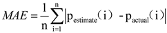
Kepler optimization algorithm is a heuristic optimization algorithm proposed by Abdel-Basset et al. [40]. In KOA, the Sun and the planets rotating around the Sun in elliptical orbits can be used to represent the search space. Since the positions of the planets (the candidate solutions) relative to the Sun (optimal solution) change over time, the search space can be explored and utilized more efficiently. During the optimization process, KOA will apply the following rules:
(1) The orbital periods of planets (the candidate solutions) are randomly selected from a normal distribution.
(2) The eccentricity of planets (the candidate solutions) is generated randomly within the range of [0,1].
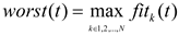
(3) The fitness of each solution is calculated based on the objective function.
(4) In the iterative process, the best solution serves as the central star (sun).
(5) Planets move around the Sun in elliptical orbits, resulting in changes in their distance over time.
Based on the above rules, after evaluating the fitness of the initial set, KOA runs iteratively until a termination criterion is met. Theoretically, KOA can be regarded as a global optimization algorithm due to its exploration and exploitation phases. The following is a detailed description of KOA’s iterative process from a mathematical point of view.
Step 1. Initial process:
The population size, denoted as N in this process, will be randomly distributed in d dimensions according to formula (1), representing the decision variables of an optimization problem.
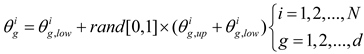 where denotes the g-th planet (candidate solution) in the search space,it represents the number of candidate solutions in the search space; represents the dimension of the problem to be optimized; and denote the upper and lower bounds of the g-th decision variable, respectively; And denotes a randomly generated number at [0,1].
The g-th planet (candidate solution) in the search space is denoted by , where represents the total number of candidate solutions in the search space. The dimension of the problem to be optimized is represented by . and denote the upper and lower bounds of the g-th decision variable respectively. Additionally, represents a randomly generated number within the range [0,1].
For each object’s orbital eccentricity (e), it is initialized as in formula (2):
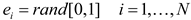 where is a randomly generated number whose value ranges from [0,1].
Finally, for the orbital period of each planet (candidate solution), it is initialized as formula (3):
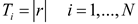 where is a randomly generated number according to a normal distribution.
Step 2. Define the force of gravity (F):
The law of universal gravitation gives the gravitational pull of the Sun and any planet . Gravity is defined as formula (4):
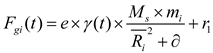
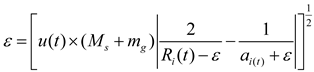
In the formula for gravitation, is a small number; is the cosmological gravitational constant; e is the eccentricity of planetary orbits, whose value ranges from [0,1], which can give KOA model more random features; is a randomly generated value between [0,1], which can provide more variation in the optimization process; are the normalized value of , which offers the Euclidean distance between the Sun and the planets , which is defined as formula (5):
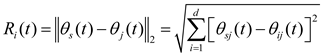 where offers the Euclidean distance between the Sun’s dimensions and the planets’ dimensions . The masses of the Sun and the planets at time can be calculated using the following formulas (6)-(7):
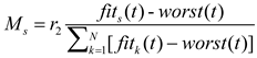
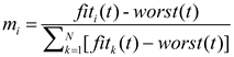 were the functions and are defined as formulas (8)—(9):
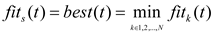
In the definition of solar mass , a random constant from 0 to 1 is generated to represent the planet’s mass value within the scatter search space. The function , which decreases exponentially with time to control the search accuracy, is defined as formula (10):
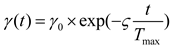 where is a constant; is an initial value, while and are the current iteration number and the maximum iteration number, respectively.
The specific motion is shown in Figure 1.
Step 3. Calculate the planet’s velocity:
The planetary velocity depends on its setting relative to the Sun , and the closer you are to the Sun , the greater the velocity; The further away from the Sun , the slower it will be. This is understood to mean that as the gravity of the Sun tries to capture the planet , the planet increases its speed to avoid being pulled closer and slows down as it escapes. Mathematically, it is understood as the process of KOA escaping from a local optimum solution, which can be described by the following formulas (11)—(20):
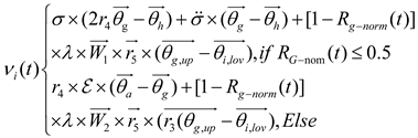

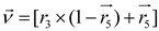
 where the velocity of the planet at a given time is represented by , while represents the planet . and are randomly generated numbers within the range [0,1], while and are random vectors contained in [0,1]. and represent a randomly selected solution from the population. and denote the masses of the Sun and planets, respectively; refers to the universal gravitational constant, while is a small value used to prevent division errors caused by zero frequency. denotes the distance between the optimal solution and the object at a specific time. Let represent the semi-major axis of the planet ’s elliptical orbit at that time, which is defined by Kepler’s third law as shown in the following formula (21):
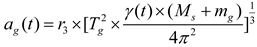 where denotes the orbital period of the planet . In our proposed algorithm, it is assumed that the semi-major axis of the elliptical orbit of the planet gradually decreases with time. That is, its solution moves toward the region where the global optimal solution is expected to be found. Let denote the Euclidean distance between the normalized and , which is defined as formula (22):
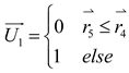
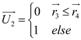
The purpose of is to calculate the percentage of time steps each object will change. If , the object is close to the Sun and will increase its speed to prevent drifting towards the Sun due to its huge gravitational pull. Otherwise, the planet will slow down.
Step 4. Escape the local optimum solution:
In the solar system, most objects rotate on their own axis while rotating counterclockwise around the Sun ; However, some objects do the opposite, rotating clockwise around the Sun. KOA mimics this mechanism by using this behavior to escape the local algorithm optimal region, which is mainly embodied by a sign F that changes the search direction, thus giving the agent a good chance to scan the search space accurately.
Step 5. Update the object position:
Based on the previous section, the planet will rotate in an elliptical orbit around the Sun. During this process, the object will move closer to the Sun for some time and away from it. The KOA algorithm simulates this behavior mainly using two phases: exploration and exploitation. KOA will explore objects far from the Sun to find new solutions and, more accurately, find the optimal solution. In this way, the exploration and exploitation area around the Sun is expanded. In the exploration phase, the target is far away from the Sun (the optimal solution), and the whole search area can be explored more effectively. Target distance from the Sun (global optimal solution).
The position update formula is as formula (23):
 where is the new position of the object in time , is the speed needed for the planet to reach the new position, is the best position of the Sun found so far, and is used as a sign to change the direction of the search. The position update formula simulates the gravitational force exerted by the Sun on the planets. In this formula, a time step is introduced based on the calculation of the distance between the current planet and the Sun, multiplied by the gravity of the Sun. This modification aids KOA in exploring its surrounding area after initialization, facilitating a more efficient searches for optimal solutions with fewer function evaluations. In general, when the planet is moving away from the Sun, the velocity of the planet will represent KOA’s exploration operator. However, this speed is affected by the Sun’s gravitational pull, which contributes to the region around the current better optimal solution for the planet. At the same time, as a planet approaches the Sun, its speed will increase dramatically, allowing it to escape the Sun’s gravitational pull. In this case, if the Sun (the optimal solution) is the local minimum, the velocity represents the local optimal avoidance, while the Sun’s gravitational representation helps KOA attack the best solution so far to find a better solution.
Step 6. Update the position with the Sun:
If the distance between the Sun and the planet is infinitesimally small, then either the planet or the Sun emerges as the optimal solution during iterative processes.
This principle is randomly swapped with the formula. The position update formula further improves KOA’s exploration operator, as shown in Step 5. The mathematical model of the principle is described as formula (24):
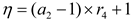
 where is an adaptive factor that controls the distance between the Sun and the current planet at the time , which is defined as formula (25):
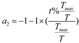
 where is a randomly generated number according to a normal distribution, and is a [-2,1] linear decreasing factor, defined as formula (26):
 where is a cyclic control parameter and gradually reduced from −2 to −1 throughout the optimization process with period as formula (27):
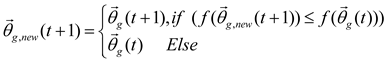
Step 7. Adjust the parameters:
This step implements an elite strategy to ensure the best placement of the planets and sun. Use the formula (28) summarizes the process:
Thus, the specific flow chart of this method is as Figure 2:
2.3. The BiGRU Model
LSTM is developed from RNN, which changes the neurons in the hidden layer of RNN through the gate mechanism and introduces a self-loop mechanism on the basis of it to improve the shortcomings of gradient disappearance. As a variant of LSTM, the GRU neural network has been optimized in structure, reducing the training time while ensuring high accuracy prediction. Compared with LSTM, GRU is more concise in design, and its structure contains only two gates: reset gate () and update gate (). The former mainly control data (or variables?). The input of data and the composition of previous memory; And the latter controls the preservation of the previous memory. The simplified structure of GRU enables it to model sequences for the temporal characteristics of data effectively while maintaining high computational efficiency. The following formulas (29)—(30) show the governing formulas for GRU units:
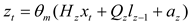
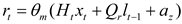 where, in Equations (8) and (9), , , , , and the corresponding activation functions as well as the bias , , update and reset gate are calculated based on the assigned weights. In addition, is the input to the neuron at the time step; and is the cell state vector at time step . After this, the reset gate is used to start new memory contents. The Hadamard (element product) is calculated using the formula . The reset gate is used to determine what information to eliminate from the previous step. After that, the activity function is applied to produce a new cell state vector .
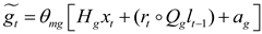
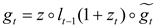
Finally, the current cell state vector is obtained by passing the reservation information to the next cell. To this end, updating the gate involves the formulas (31)—(32):
For information retrieval and storage, the GRU neural network adopts a recurrent structure. Still, this structure only considers the previous state of the prediction point, ignoring the future state of the prediction point. However, in actual forecasting, the load information at the previous time is always highly related to the load information at the next time. Therefore, the prediction accuracy cannot be further improved. For deeper time series feature extraction, BiGRU is introduced here.
BiGRU (Bidirectional Recurrent Neural Network) consists of a forward GRU layer and an inverse GRU layer, which allows for predicting time series in the opposite direction. In the end, the output will be determined by the state of the forward and inverse layers. Due to the absence of a connection between the forward and inverse layers, BiGRU enables simultaneous consideration of data change patterns compared to one-way GRU, thereby enhancing flexibility, comprehensiveness, and relevance in analysis. This promotes a stronger integration between the model and its processing information while significantly improving prediction accuracy as compared to GRU. The structure of BiGRU is shown in Figure 3 and the expression of the network structure is as formula(33)—(35).
 where GRU is the traditional GRU network operation process, and are the state and weight of the forward hidden layer at time ; and are the state and weight of the backward hidden layer at time ; and is the bias of the hidden layer at time .
The specific structure of BiGRU is shown in Figure 3.
2.4. BiTCN Model
The Time Convolutional Network (TCN) models have gained significant attention and application in the field due to their ability to process time series data in parallel efficiently. Similarly, the study and application of BiLSTM networks have been validated to capture important fluctuation characteristics associated with future time parameters. However, it should be noted that in predicting the current power load, TCN is limited to capturing past parameter fluctuations such as wind speed, temperature, and rate of change. In summary, this paper proposes to optimize the power load forecasting model by BiTCN algorithm.
The BiTCN model facilitates bidirectional information integration by simultaneously capturing the fluctuation characteristics of parameter changes in both past and future time dimensions. It achieves this by connecting forward TCN modules, backward TCN modules, and a temporal attention module within each BiTCN module. Multiple BiTCN modules are sequentially connected to construct the overall BiTCN model.
The forward TCN model receives past time parameters as inputs from the module, while the backward TCN model takes future time parameters as inputs. Both models share consistent input parameters and employ temporal attention to merge and process the outputs from both modules, resulting in a novel set of output features. Element-wise input fusion significantly enhances the performance of the model.
We are assuming that the input to the modulein the BiTCN model is , where . Firstly, is fed into the forward TCN module to extract historical temporal information from the vibration data and obtain bold time features . Simultaneously, by applying reverse processing on , we accept backward time data , where . Then, it serves as input for the back TCN module to extract future temporal information from the vibration data and acquire backward time features . The formulas for calculating these two types of features are as formulas (36)—(37):
The dimensions of the temporal convolutional kernel for capturing time gaps, the parameter for Leaky ReLU activation function, the dilation rate for atrous convolution, and the parameter for Dropout regularization are represented by , , , and , respectively. denotes feature extraction in the forward TCN module while describes feature extraction in the backward TCN module.The structure of BiTCN is shown as Figure 4.
2.5. The Attention Mechanism
The attention mechanism is a computational approach that emulates the information processing mechanism of the human brain, thereby enhancing the information processing capability of neural networks. It selectively emphasizes important features by assigning weights to input features and applying weight distribution to retain intermediate results in neural network computations. This facilitates learning with a new model while reducing or disregarding the influence of irrelevant features, thus achieving effective information filtering, improving analysis efficiency, enabling better decision-making by models, and enhancing prediction accuracy. For short-term load forecasting tasks, models often need to process large volumes of load data within limited time frames. The value of the load at a specific moment is more closely related to nearby load values than those further away. Therefore, models should primarily focus on recent load values during prediction. This necessitates leveraging attention mechanisms. The attention mechanism can assign varying weights to each time point’s load value by giving higher weights to values closer in time and lower weights as they become more distant from the current time point. Consequently, models can effectively capture valuable information quickly and improve prediction accuracy. Figure 5 illustrates the structure of an attention mechanism representing an attention distribution vector.
The relevant formulas for this mechanism are as formulas (38)–(40):

The attention scoring function is in the hidden layer , while and represent the attention weights. denotes the bias term, and signifies the dimensionality of input vectors.
2.6. Construction of KOA-BiGRU-BiTCN-Attention Model
To sum up, we can construct the integrated Attention mechanism and the BiGRU-BiTCN algorithm optimized by the KOA optimization algorithm as shown in Figure 6:
3. Results and Discussion of KOA-BiGRU-BiTCN-Attention Model
To verify the accuracy and generality of the model, this paper selects the wind power dataset from Xinjiang, China, for a verification experiment and a comparison experiment.
3.1. Example of Xinjiang Wind Power Data
This paper utilizes a total of 35,040 load data points from Xinjiang wind power, spanning from January 1, 2019, to December 30, 2019, along with related meteorological and temporal data, to construct and verify a power load prediction model. The power load data have a sampling interval of 15 min, resulting in 96 data points sampled each day. For short-term prediction, we selected the first 34,960 data points as the training dataset and the last 100 data points as the validation dataset. For long-term prediction, the first 28,040 data points were chosen as the training dataset, and the previous 7000 data points served as the validation dataset.
3.1.1. Data Preprocessing
By checking the data set, it is found that the data set has missing values. The specific missing values are listed in the following Table 1:
Accordingly, we use the KNNI algorithm to fill the vacancy value:
First, we randomly delete a part of the data on the complete time series to simulate the missing value through program processing and use the KNNI algorithm to perform a filling simulation to test the model performance, as follows Figure 7 and Table 2:
Then, we apply the model to fill the corresponding vacancy value. Next, we carry out the subsequent screening and variable prediction.
3.2. Selection of Input Variables
After the correlation analysis of different wind speeds, wind direction, and other variables with load data, this paper selected the nine variables with the highest correlation as input variables to train the model and forecast the future load data. The specific data and results are as follows Figure 8:
Previous studies have shown that deep learning models are more sensitive to numbers between 0 and 1 [20]. Therefore, the original load sequence is input. Before entering the MapReduce-BP model, the load data is normalized first, and then the inverse normalization is processed after the training to get the actual load forecast value.
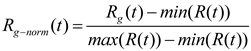
3.3. Selection of Evaluation Indicators
In order to quantitatively evaluate the accuracy of the prediction model, we use three leading evaluation indicators in this paper. These include mean absolute error, which measures the mean fundamental difference between the predicted value and the actual value; The mean fundamental percentage error, which provides the expected error as a percentage of the true value, allowing us to understand the effect of the error in the aggregate; And root-mean-square error, which is the square root of the mean of the squared prediction error and is able to give the magnitude of the prediction error. The specific calculation formulais as follows:
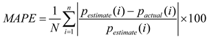
 where and are the predicted value and the measured value, respectively, and are the average values of the predicted and measured values, respectively.
3.4. Setting of Model Parameters
Before the experiment starts, we first set the parameters of the relevant model and its optimization algorithm. The relevant parameters of the KOA optimization algorithm are as follows Table 3:
The relevant parameters of the BiGRU-BiTCN-Attention optimization algorithm are as follows Table 4:
3.5. Load Forecasting Experiment Platform and Result Analysis
3.5.1. Experimental Platform
The experiments described in this paper are run on GPU, the graphics card is NVIDIA GeForce GTX 3060, and the experimental environment is MATLAB 2023a edition.
3.5.2. Analysis of Ablation Experiment Results
In this experiment, the prediction results of TCN, GRU, TCN-GRU, and BiTCN-BiGRU prediction methods were taken as the comparison reference, recorded as the experimental control group, and compared with the prediction results of the proposed model to confirm the following two points:
(1) The feature capture efficiency and prediction accuracy of BiTCN-BiGRU are superior to the basic BiTCN, BiGRU, TCN and GRU prediction methods.
(2) KOA, as a population optimization algorithm, can effectively improve the adjustment efficiency and prediction accuracy of hyperparameters.
Therefore, on the experimental platform, we conducted relevant experiments and obtained the following results Table 5 and Figure 9:
P.S: Bbmeans BiGRU-BiTCN, BBA means BiGRU-BiTCN-Attention
The experimental results show that:
The initial model is a network based on a gated cycle unit (GRU), which has the worst performance on all evaluation indicators, including RMSE (31.71%), MAPE (39.53%), and MAE (31.99). After the introduction of the temporal convolutional network (TCN), RMSE, MAPE, and MAE of the model improved by 11.38%, 19.48%, and 24.04%, respectively, indicating that TCN has a significant advantage in capturing long-term dependencies of time series. The bidirectional GRU (BiGRU) and bidirectional TCN (BiTCN) structures are further used to improve the model performance. Compared with unidirectional TCN, the BiTCN model enhanced by 8.08%, 3.31%, and 6.23% in RMSE, MAPE, and MAE, respectively. The TCN-GRU model combined with TCN and GRU also showed improved performance compared with the single BiTCN model, with RMSE increased by 6.81%. Further, the BITCN-BiGRU-Attention model formed by combining BiTCN and BiGRU and introducing the attention mechanism has achieved significant performance improvement in all evaluation indicators, among which RMSE, MAPE, and MAE have increased by 8.92%, 28.04%, and 24.49%, respectively. This indicates that the attention mechanism can effectively enhance the model’s ability to recognize essential features in time series, thus improving the prediction accuracy. The KOA-BiTCN-BiGRU-Attention model with the introduction of the KOA mechanism achieved the most significant improvement in all indicators, among which RMSE, MAPE, and MAE improved by 22.87%, 43.48%, and 30.61%, respectively. The above experiments verify the performance of the proposed model.
At the same time, in order to verify the optimization efficiency of the KOA optimization algorithm, this paper selected the BiTCN-BiGRU-Attention model optimized by TSA, SMA, GWO, and WOA optimization algorithms for performance comparison. The relevant algorithms are introduced as follows:
The Tunicate Swarm Algorithm (TSA) is a new optimization algorithm proposed by Kaur et al. It is inspired by the swarm behavior of the capsule to survive successfully in the deep sea. The TSA algorithm simulates the jet propulsion and swarm behavior of the capsule during navigation and foraging. This algorithm can solve relevant cases with unknown search space [43].
The slime mold algorithm is an intelligent optimization algorithm proposed in 2020, which mainly simulates the foraging behavior and state changes of physarum polycephalum in nature under different food concentrations. Myxomycetes primarily secrete enzymes to digest food. The front end of myxomycetes extends into a fan shape, and the back end is surrounded by a network of interconnected veins. Different concentrations of food in the environment affect the flow of cytoplasm in the vein network of myxomycetes, thus forming other states of myxomycetes foraging [30].
Grey Wolf Optimizer (GWO) is a population intelligent optimization algorithm proposed in 2014 by Mirjalili et al., scholars from Griffith University in Australia. This algorithm is an optimization search method developed inspired by the prey-hunting activities of grey Wolves [44].
The Whale Optimization Algorithm (WOA) is a new swarm intelligence optimization algorithm proposed by Mirjalili and Lewis from Griffith University in Australia in 2016. Inspired by the typical air curtain attack behavior of humpback whales in the process of simulating simple prey, WOA optimized the relevant process [45].
According to the experimental results, the KOA-BiTCN-BiGRU-Attention model outperforms other variant models on all evaluation indexes. Specifically, compared with the TSA-BiTCN-BiGRU-Attention model, the KOA variant achieved 10.53%, 15.95%, and 11.92% improvement in RMSE, MAPE, and MAE, respectively. Similarly, compared to the SMA-BiTCN-BiGRU-Attention model, the KOA variant achieved a 13.15%, 35.32%, and 20.51% improvement on these three metrics, respectively. In addition, compared with the GWO-BiTCN-BiGRU-Attention and WOA-BiTCN-BiGRU-Attention models, the KOA variant also showed outstanding improvement in RMSE, MAPE, and MAE, reaching 12.32%, 14.47%, 12.21%, 16.19%, 25.58%, and 17.06%, respectively. This proves that the KOA optimization algorithm has obvious advantages over traditional optimization methods.
Then, this paper selects the classical model and sets the relevant parameters consistent with the model proposed in this paper for comparative experiments. The types of models are as follows: Decision Tree: A decision tree builds a tree-like model of decision rules by recursively splitting the data set into smaller subsets. Each internal node represents a test on an attribute, each branch represents the result of the test, and each leaf node represents a prediction result. In time series forecasting, the decision tree can predict a target value at a future point in time based on the eigenvalue at a past point in time.
XGBoost: XGBoost is an efficient gradient lifting library that uses the Gradient lifting (GBM) framework. XGBoost adds trees at each step to minimize the loss function, which is used to measure the difference between the predicted and actual values of the model. XGBoost has regularization capabilities that help reduce the overfitting of the model, resulting in improved prediction accuracy in time series predictions. Gaussian Regression: Gaussian regression is a regression method based on Gaussian processes that incorporate prior knowledge of the infinite-dimensional space of the function into the model, learning this distribution through observations of the training data. In time series forecasting, Gaussian regression can take advantage of its smoothing properties to predict continuous time series data.
Extreme Learning Machine Regression (ELM): ELM is a learning algorithm proposed for single-hidden layer feedforward neural networks. Its core idea is to initialize the weight and bias of the hidden layer randomly and then directly calculate the weight of the output layer using an analytical method. This method reduces the number of parameters that need to be adjusted, thus speeding up the learning speed, and is especially suitable for fast prediction of time series data.
GRNN (Generalized Regression Neural Network): A GRNN is a neural network based on kernel regression that calculates the distance of each input vector from every sample in the training set and then estimates the output value based on those distances. GRNN is particularly well suited for dealing with noisy datasets and nonlinear problems, making it a powerful tool for time series prediction.
Generalized Additive Models Regression (GAM): GAM models the relationship between response and predictor variables by adding the sum of multiple smoothing functions, one predictor for each smoothing function. This model structure makes GAM both flexible and easy to interpret, making it ideal for solving complex nonlinear relationships in time series data.
SVR (Support Vector Regression): SVR uses the same principles as support vector machines, but the goal in regression problems is to have the data points fall within the ε band of the decision boundary defined by the support vector as much as possible. The SVR makes the model more robust by introducing relaxation variables to handle situations where it is impossible to fall entirely within the ε band.
BP (Back Propagation Neural Network): The BP algorithm updates the weight and bias of the network by calculating the error between the prediction and the actual output and propagating this error backward through the network. This approach allows multilayer feedforward neural networks to be able to learn complex non-linear relationships, making it a powerful tool in time series prediction.
LSTM (Long Short-Term Memory): LSTM controls the flow of information by introducing three gates (input gate, forget gate, and output gate), which allows it to eliminate or mitigate the gradient disappearance problem in traditional RNNS, thus effectively capturing long-term dependencies. This property makes LSTM suitable for time series prediction, especially when predicting long-time series.
LSTM-CNN (Long Short-Term Memory Convolutional Neural Network): LSTM-CNN exploits LSTM’s ability to process sequence data and CNN’s advantage in feature extraction by combining LSTM with CNN. This combination can effectively process the spatio-temporal features in the time series data, thus improving the prediction accuracy.
MLP (Multi-Layer Perceptron): MLP is able to capture complex nonlinear relationships by introducing one or more hidden layers and using nonlinear activation functions to increase the expressive power of the network. This makes MLP a powerful tool for dealing with time series prediction problems, especially when complex non-linear patterns are present in the data.
The MLP-DT(Ensemble Learning) ensemble learning method combines the strengths of Multilayer Perceptron (MLP) and Decision Tree (DT) regression models to enhance overall predictive performance and generalization ability. First, MLP and DT are selected as base models due to their superior predictive performance. Next, a hyperparameter space is defined for each model, and model training is conducted on the training set while continuously tuning hyperparameters on the validation set to find the optimal models and record validation errors. Finally, the validation errors of different models are compared; if the error differences are significant, the model with the smaller error is selected. If the errors are within a certain threshold, the predictions of the two models are combined using weighted averaging. The final prediction is the weighted sum of the two models’ predictions.
P.S: DT means Decision Tree
In all the above evaluation indicators, the KOA-BiTCN-BiGRU-Attention model showed significant performance improvement compared with other models. Compared with the ELM model, the improvement percentage of KOA-BiTCN-BiGRU-Attention on RMSE, MAPE, and MAE was 76.80%, 73.46%, and 79.67%, respectively, showing excellent performance for processing very complex time series data. In addition, compared with the classical LSTM model, the improvement of the KOA-BiTCN-BiGRU-Attention model in these three indicators reached 71.12%, 74.02%, and 76.01%, respectively, which had different degrees of improvement compared with other models. This further proves the advanced nature and high efficiency of the model proposed in this paper.
The specific improved performance visualization is as follows Figure 12:
P.S: TG means TCN-GRU, CL means CNN-LSTM
In summary, this section verifies the performance of the proposed 24-step multi-variable time series short-term load forecasting model. At the same time, we will further study the model in the future to improve its relevant performance and calculation speed.
3. Conclusions
Electricity demand forecasting, a field of long-standing research, has developed various mature prediction models and theories. With the advancement of global “carbon peak and carbon neutrality” goals and the implementation of numerous carbon reduction policies, certain high-energy-consumption and high-emission industries face restrictions or even transformation, while new green industries are emerging rapidly. These changes have led to significant adjustments in China’s industrial structure, rendering traditional methods based on historical data inadequate. Furthermore, in the context of the construction of new electricity markets, the structure of power systems has become increasingly complex, enabling bi-directional interactions between electricity and information flow, and allowing demand-side resources to participate in grid peak shaving and frequency modulation, directly affecting grid loads. Therefore, considering the impacts of “dual carbon” goals and the construction of new power systems is particularly important in mid-to-long-term electricity demand forecasting. Given the differences in principles, advantages, and applicable scenarios of various prediction models, the selection and optimization of models are crucial to ensure adaptability to the complex power system environment under the influence of “dual carbon” goals. Against this backdrop, this study has arrived at the following main conclusions and achievements:
1) A novel algorithmic model for short-term load forecasting in 24-step multivariate time series has been proposed. This model combines KNN data imputation with BiTCN bidirectional temporal convolutional network, along with BiGRU bidirectional gated recurrent unit and attention mechanism. Furthermore, the model’s hyperparameters have been optimized using Kepler Adaptive Optimization Algorithm (KOA), resulting in enhanced prediction accuracy compared to equivalent time steps.
2) An integrated approach has been adopted by combining different models to construct a comprehensive short-term electricity load forecasting model. This holistic framework not only provides valuable insights for production-related decisions but also serves as a reference point for formulating and implementing relevant policies.
Author Contributions
Conceptualization, M.X. and W.L.; methodology, M.X.; software, M.X.; validation, S.W., J.T., and P.W.; formal analysis, M.X.; investigation, S.W.; resources, P.W.; data curation, J.T.; writing—original draft preparation, M.X.; writing—review and editing, J.T. and W.L.; visualization, J.T. and C.X.; supervision, P.W.; project administration, J.T.
Funding
This research received no external funding.
Data Availability Statement
Due to the confidentiality agreement signed with the relevant enterprises, the relevant data cannot be disclosed, please understand.
Acknowledgments
Thanks to Teacher Peng Wu for the experimental guidance of this paper.
Conflicts of Interest
The authors declare no conflicts of interest.
References
- Petrušić, A.; Janjić, A. Fuzzy Multiple Linear Regression for the Short Term Load Forecast. In Proceedings of the 2020 55th International Scientific Conference on Information, Communication and Energy Systems and Technologies, Niš, Serbia, 10–12 September 2020. [Google Scholar] [CrossRef]
- Yang, G.; Zheng, H.; Zhang, H.; Jia, R. Short-term load forecasting based on holt-winters exponential smoothing and temporal convolutional network. Dianli Xitong Zidonghua/Autom. Electr. Power Syst. 2022, 46, 73–82. [Google Scholar] [CrossRef]
- Yakhot, V.; Orszag, S.A. Renormalization group analysis of turbulence. I. Basic theory. J. Sci. Comput. 1986, 1, 3–51. [Google Scholar] [CrossRef]
- Vaish, J.; Siddiqui, K.M.; Maheshwari, Z.; Kumar, A.; Shrivastava, S. Day Ahead Load Forecasting using Random Forest Method with Meteorological Variables. In Proceedings of the 2023 IEEE Conference on Technologies for Sustainability (SusTech), Portland, OR, USA, 19–22 April 2023. [Google Scholar] [CrossRef]
- Ding, Q. Long-Term Load Forecast using Decision Tree Method. In Proceedings of the 2006 IEEE PES Power Systems Conference and Exposition, Atlanta, GA, USA, 29 October–1 November 2006. [Google Scholar] [CrossRef]
- Zhang, T.; Huang, Y.; Liao, H.; Liang, Y. A hybrid electric vehicle load classification and forecasting approach based on GBDT algorithm and temporal convolutional network. Appl. Energy 2023, 351, 121768. [Google Scholar] [CrossRef]
- Lu, K.; Sun, W.; Ma, C.; Yang, S.; Zhu, Z.; Zhao, P.; Zhao, X.; Xu, N. Load forecast method of electric vehicle charging station using SVR based on GA-PSO. IOP Conf. Ser.: Earth Environ. Sci. 2017, 69, 012196. [Google Scholar] [CrossRef]
- Huang, A.; Zhou, J.; Cheng, T.; He, X.; Lv, J.; Ding, M. Short-term Load Forecasting for Holidays based on Similar Days Selecting and XGBoost Model. In Proceedings of the 2023 IEEE 6th International Conference on Industrial Cyber-Physical Systems, Wuhan, China, 8–11 May 2023. [Google Scholar] [CrossRef]
- Zhang, W.; Hua, H.; Cao, J. Short Term Load Forecasting Based on IGSA-ELM Algorithm. In Proceedings of the 2017 IEEE International Conference on Energy Internet, Beijing, China, 17–21 April 2017. [Google Scholar] [CrossRef]
- Hu, Y.; Qu, B.; Wang, J.; Liang, J.; Wang, Y.; Yu, K.; Li, Y.; Qiao, K. Short-term load forecasting using multimodal evolutionary algorithm and random vector functional link network based ensemble learning. Appl. Energy 2021, 285, 116415. [Google Scholar] [CrossRef]
- Aseeri, A.O. Effective RNN-based forecasting methodology design for improving short-term power load forecasts: Application to large-scale power-grid time series. J. Comput. Sci. 2023, 68, 101984. [Google Scholar] [CrossRef]
- Ajitha, A.; Goel, M.; Assudani, M.; Radhika, S.; Goel, S. Design and development of residential sector load prediction model during COVID-19 pandemic using LSTM based RNN. Electr. Power Syst. Res. 2022, 212, 108635. [Google Scholar] [CrossRef]
- Fang, P.; Gao, Y.; Pan, G.; Ma, D.; Sun, H. Research on forecasting method of mid- and long-term photovoltaic power generation based on LSTM neural network. Renewable Energy Resour. 2022, 40, 48–54. (in Chinese). [Google Scholar] [CrossRef]
- Zhang, Q.; Tang, Z.; Wang, G.; Yang, Y.; Tong, Y. Ultra-short-term wind power prediction model based on long and short term memory network. Acta Energiae Solaris Sinica 2021, 42, 275–281. (in Chinese). [Google Scholar] [CrossRef]
- Rick, R.; Berton, L. Energy forecasting model Based on CNN-LSTM-AE for many time series with unequal lengths. Eng. Appl. Artif. Intell. 2022, 113, 104998. [Google Scholar] [CrossRef]
- Fu, Y.; Ren, Z.; Wei, S.; Wang, Y.; Huang, L.; Jia, F. Ultra-short-term power prediction of offshore wind power based on improved LSTM-TCN model. Proc. CSEE 2022, 42, 4292–4303. (in Chinese). [Google Scholar] [CrossRef]
- Al-Ja’afreh, M.A.A.; Mokryani, G.; Amjad, B. An enhanced CNN-LSTM based multi-stage framework for PV and load short-term forecasting: DSO scenarios. Energy Rep. 2023, 10, 1387–1408. [Google Scholar] [CrossRef]
- Holland, J.H. Genetic algorithms. Sci. American 1992, 267, 66–73. [Google Scholar] [CrossRef]
- Kenndy, J.; Eberhart, R. Particle Swarm Optimization. In Proceedings of the ICNN’95-International Conference on Neural Networks, Perth, WA, Australia, 27 November–1 December 1995. [Google Scholar] [CrossRef]
- Dorigo, M.; Di Caro, G.; Gambardella, L.M. Ant algorithms for discrete optimization. Artif. Life 1999, 5, 137–172. [Google Scholar] [CrossRef] [PubMed]
- Rashedi, E.; Nezamabadi-Pour, H.; Saryazdi, S. GSA: A gravitational search algorithm. Inf. Sci. 2009, 179, 2232–2248. [Google Scholar] [CrossRef]
- Rao, R.V.; Savsani, V.J.; Vakharia, D.P. Teaching-learning-based optimization: A novel method for constrained mechanical design optimization problems. Comput.-Aided Des. 2011, 43, 303–315. [Google Scholar] [CrossRef]
- Wolpert, D.H.; Macready, W.G. No free lunch theorems for optimization. IEEE Trans. Evol. Comput. 1997, 1, 67–82. [Google Scholar] [CrossRef]
- Faramarzi, A.; Heidarinejad, M.; Mirjalili, S.; Gandomi, A.H. Marine predators algorithm: A nature-inspired metaheuristic. Expert Syst. Appl. 2020, 152, 113377. [Google Scholar] [CrossRef]
- Braik, M.S. Chameleon Swarm Algorithm: A bio-inspired optimizer for solving engineering design problems. Expert Syst. Appl. 2021, 174, 114685. [Google Scholar] [CrossRef]
- Hashim, F.A.; Hussain, K.; Houssein, E.H.; Mabrouk, M.S.; Al-Atabany, W. Archimedes optimization algorithm: A new metaheuristic algorithm for solving optimization problems. Appl. Intell. 2021, 51, 1531–1551. [Google Scholar] [CrossRef]
- Mohammadi-Balani, A.; Nayeri, M.D.; Azar, A.; Taghizadeh-Yazdi, M. Golden eagle optimizer: A nature-inspired metaheuristic algorithm. Comput. Ind. Eng. 2021, 152, 107050. [Google Scholar] [CrossRef]
- Shadravan, S.; Naji, H.R.; Bardsiri, V.K. The Sailfish Optimizer: A novel nature-inspired metaheuristic algorithm for solving constrained engineering optimization problems. Eng. Appl. Artif. Intell. 2019, 80, 20–34. [Google Scholar] [CrossRef]
- Khishe, M.; Mosavi, M.R. Chimp optimization algorithm. Expert Syst. Appl. 2020, 149, 113338. [Google Scholar] [CrossRef]
- Li, S.; Chen, H.; Wang, M.; Heidari, A.A.; Mirjalili, S. Slime mould algorithm: A new method for stochastic optimization. Future Gener. Comput. Syst. 2020, 111, 300–323. [Google Scholar] [CrossRef]
- Zhao, S.; Zhang, T.; Ma, S.; Chen, M. Dandelion optimizer: A nature-inspired metaheuristic algorithm for engineering applications. Eng. Appl. Artif. Intell. 2022, 114, 105075. [Google Scholar] [CrossRef]
- Abdollahzadeh, B.; Gharehchopogh, F.S.; Mirjalili, S. African vultures optimization algorithm: A new nature-inspired metaheuristic algorithm for global optimization problems. Comput. Ind. Eng. 2021, 158, 107408. [Google Scholar] [CrossRef]
- Eslami, N.; Yazdani, S.; Mirzaei, M.; Hadavandi, E. Aphid-Ant Mutualism: A novel nature-inspired metaheuristic algorithm for solving optimization problems. Math. Comput. Simul. 2022, 201, 362–395. [Google Scholar] [CrossRef]
- Zhong, C.; Li, G.; Meng, Z. Beluga whale optimization: A novel nature-inspired metaheuristic algorithm. Knowledge Based Syst. 2022, 251, 109215. [Google Scholar] [CrossRef]
- Jafari, M.; Salajegheh, E.; Salajegheh, J. Elephant clan optimization: A nature-inspired metaheuristic algorithm for the optimal design of structures. Appl. Soft Comput. 2021, 113, 107892. [Google Scholar] [CrossRef]
- Kazemi, M.V.; Veysari, E.F. A new optimization algorithm inspired by the quest for the evolution of human society: Human felicity algorithm. Expert Syst. Appl. 2022, 193, 116468. [Google Scholar] [CrossRef]
- Pan, J.S.; Zhang, L.; Wang, R.; Snášel, V.; Chu, S. Gannet optimization algorithm: A new metaheuristic algorithm for solving engineering optimization problems. Math. Comput. Simul. 2022, 202, 343–373. [Google Scholar] [CrossRef]
- Zhang, J.; Wang, S.; Tan, Z.; Sun, A. An improved hybrid model for short term power load prediction. Energy 2023, 268, 126561. [Google Scholar] [CrossRef]
- Li, D.; Ji, X.; Tian, X. Short-term Power Load Forecasting Based On VMD-GOA-LSSVR Model. In Proceedings of the 2021 China Automation Congress, Beijing, China, 22–24 October 2021. [Google Scholar] [CrossRef]
- Abdel-Basset, M.; Mohamed, R.; Abdel Azeem, S.A.; Jameel, M.; Abouhawwash, M. Kepler optimization algorithm: A new metaheuristic algorithm inspired by Kepler’s laws of planetary motion. Knowledge-Based Syst. 2023, 268, 110454. [Google Scholar] [CrossRef]
- Wang, Z.; Qiu, H.; Sun, Y.; Deng, Q. Collaborative Filtering Recommendation Algorithm Based on Random Forest Filling. In Proceedings of the 2019 2nd International Conference on Information Systems and Computer Aided Education, Dalian, China, 28–30 September 2019. [Google Scholar] [CrossRef]
- Liu, X.; Du, S.; Li, T.; Teng, F.; Yang, Y. A missing value filling model based on feature fusion enhanced autoencoder. Appl. Intell. 2023, 53, 24931–24946. [Google Scholar] [CrossRef]
- Kaur, S.; Awasthi, L.K.; Sangal, A.L.; Dhiman, G. Tunicate Swarm Algorithm: A new bio-inspired based metaheuristic paradigm for global optimization. Eng. Appl. Artif. Intell. 2020, 90, 103541. [Google Scholar] [CrossRef]
- Seyedali Mirjalili, Shahrzad Saremi, Seyed Mohammad Mirjalili, & Leandro dos S. Coelho. (2016). Multi-objective grey wolf optimizer: A novel algorithm for multi-criterion optimization. Expert Systems with Applications, 47, 106-119. [CrossRef]
- Mirjalili, S.; Lewis, A. The whale optimization algorithm. Adv. Eng. Software 2016, 95, 51–67. [Google Scholar] [CrossRef]
Figure 1.
Possible positions in (a) 2-dimension and (b) 3-dimension.
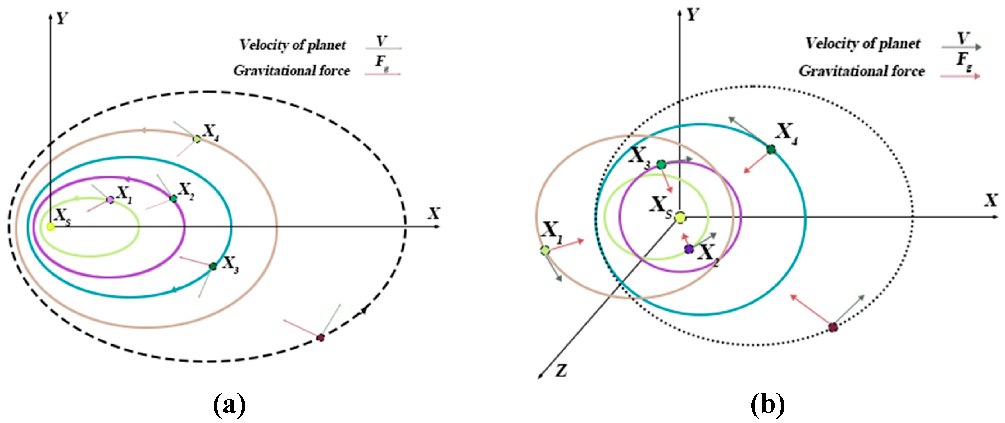
Figure 2.
Flow chart KOA optimization algorithm.
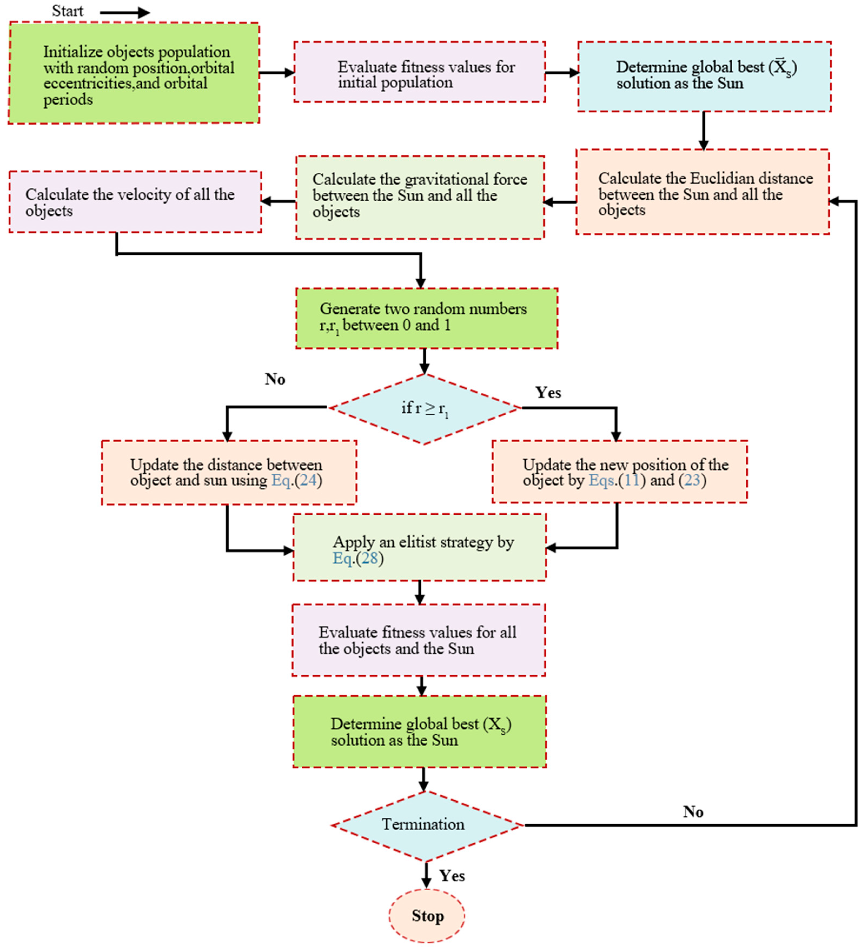
Figure 3.
Diagram of the BiGRU structure.
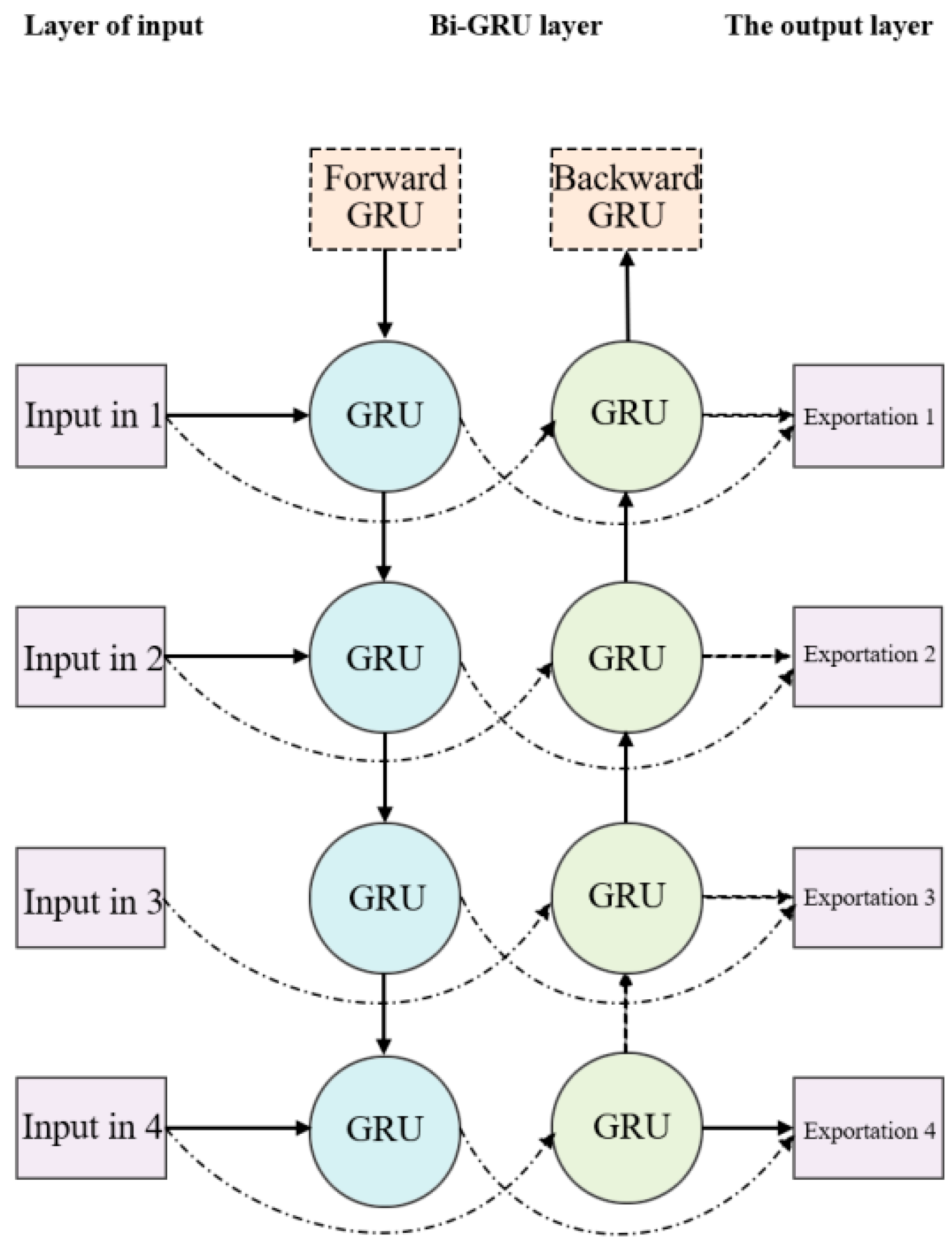
Figure 4.
BiTCN module structure.
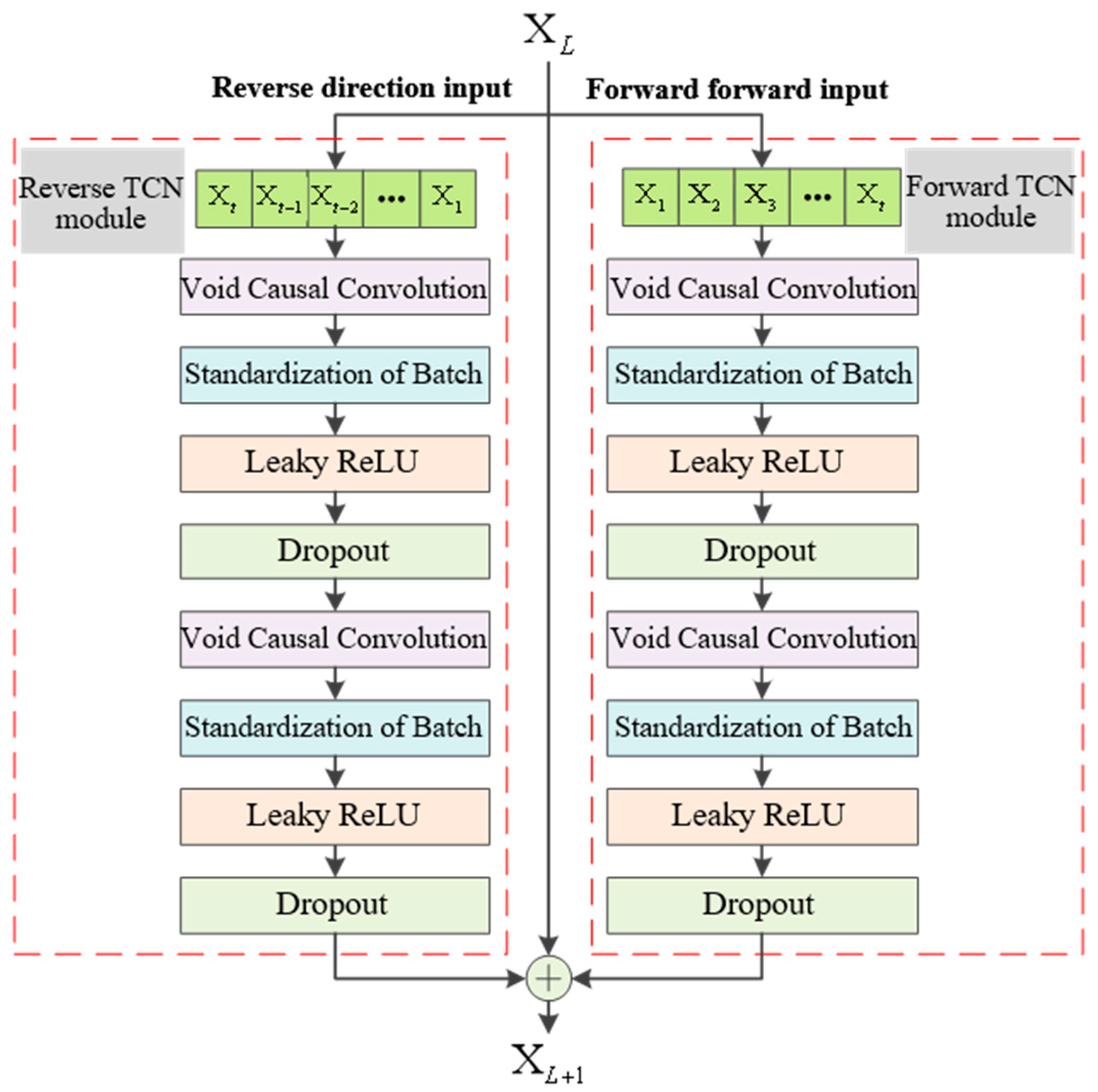
Figure 5.
Attention mechanism.
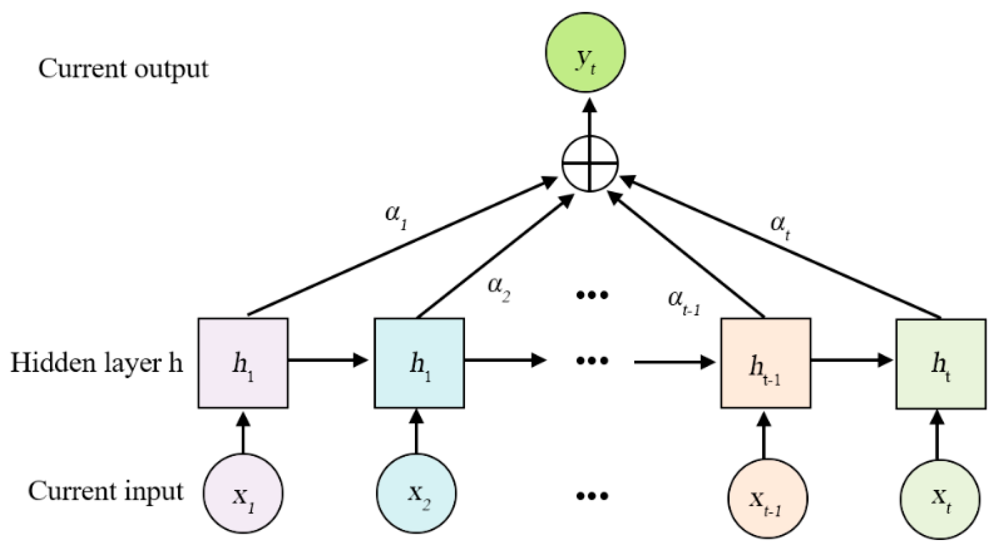
Figure 6.
Structure of KOA-BiGRU-BiTCN-Attention model.
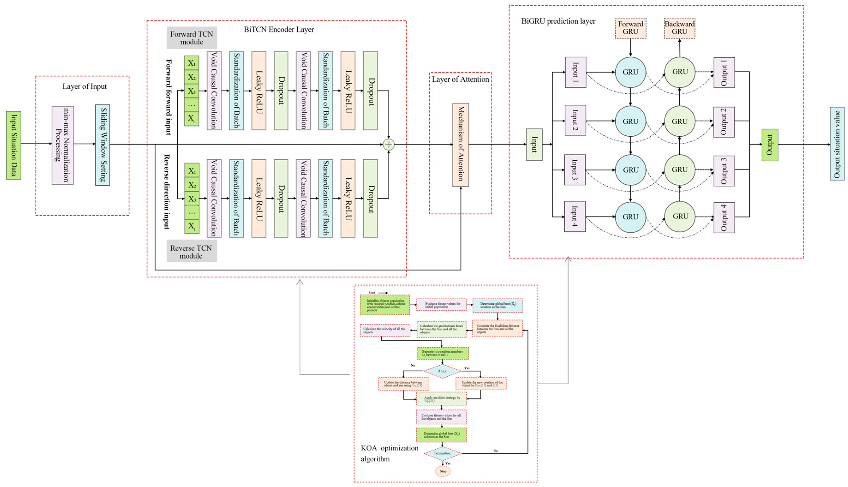
Figure 7.
Imputation of missing values for the KNNI model.
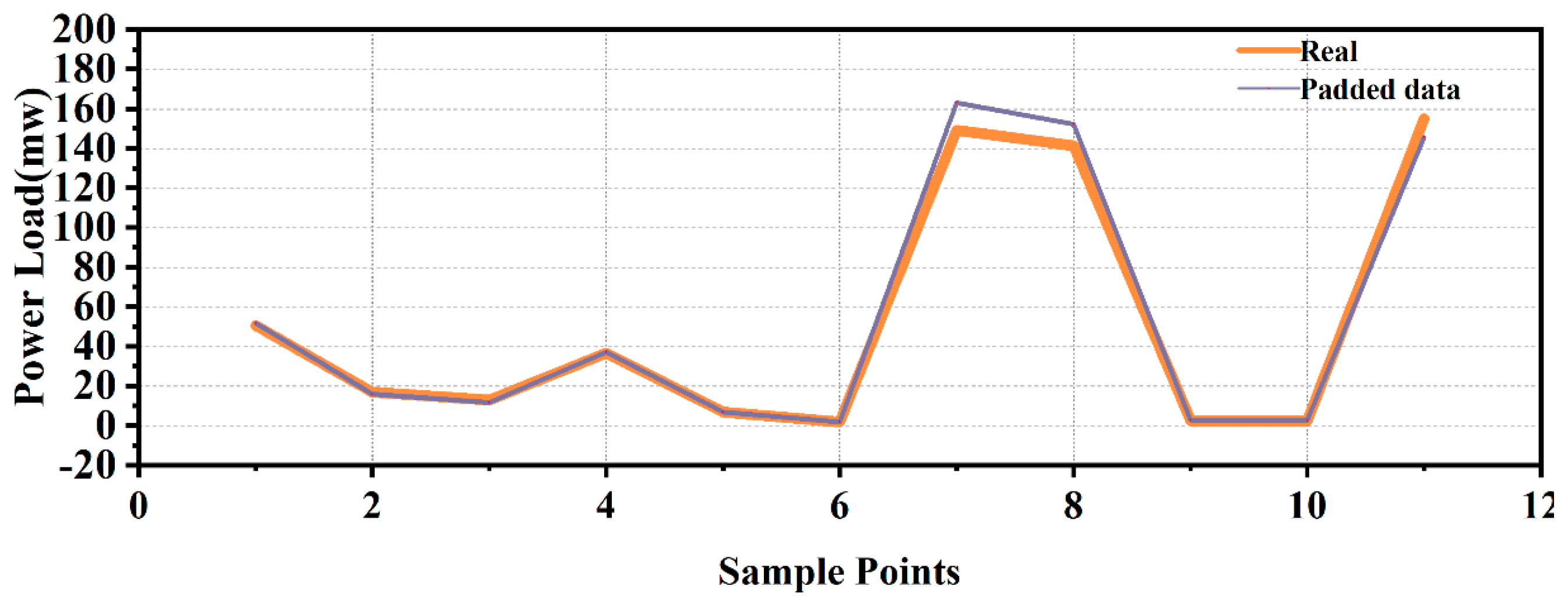
Figure 8.
Correlation heatmap.
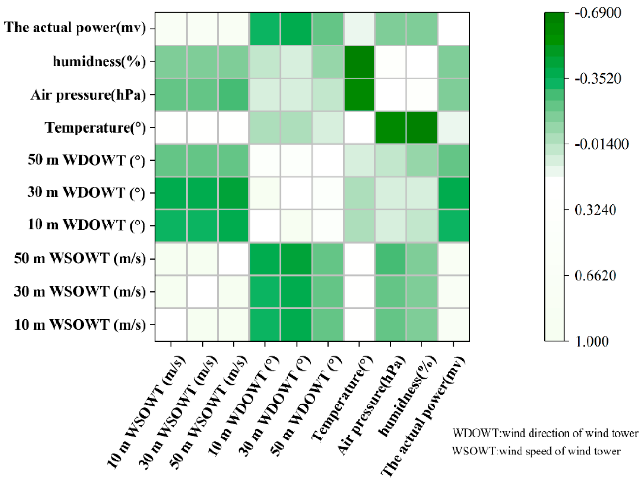
Figure 9.
Visualization of the performance of ablation experiments visualization.
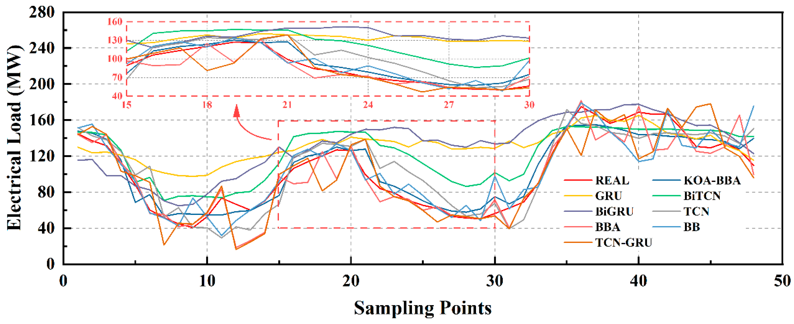
Figure 10.
Visualization of prediction results of different optimization algorithms.
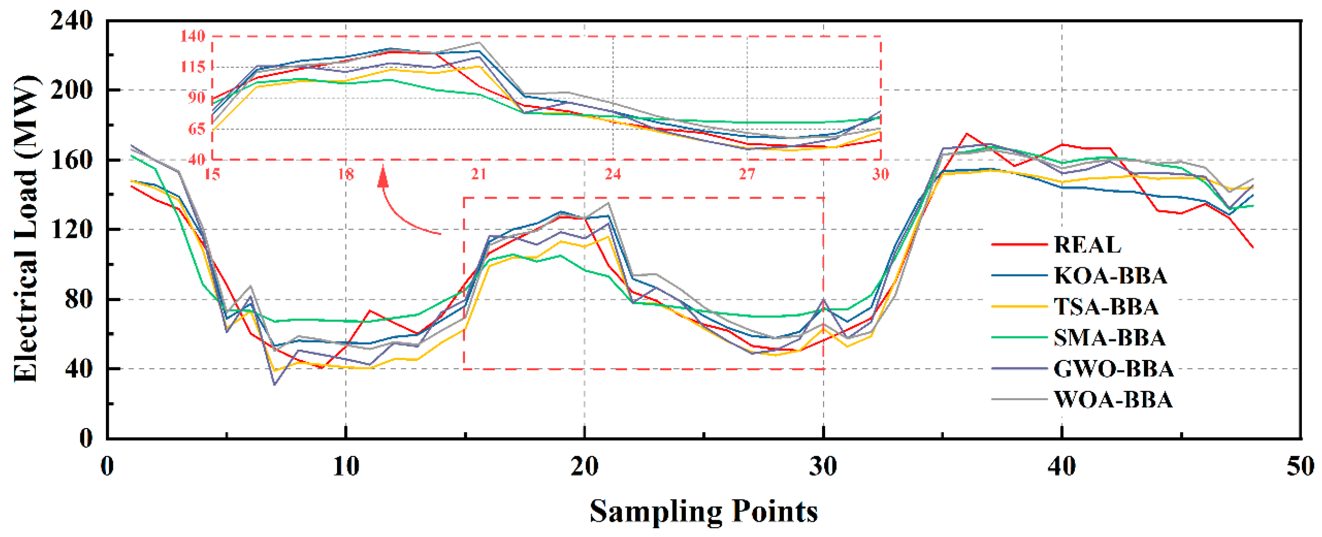
Figure 11.
Visualization of comparison of classical algorithm predictions.
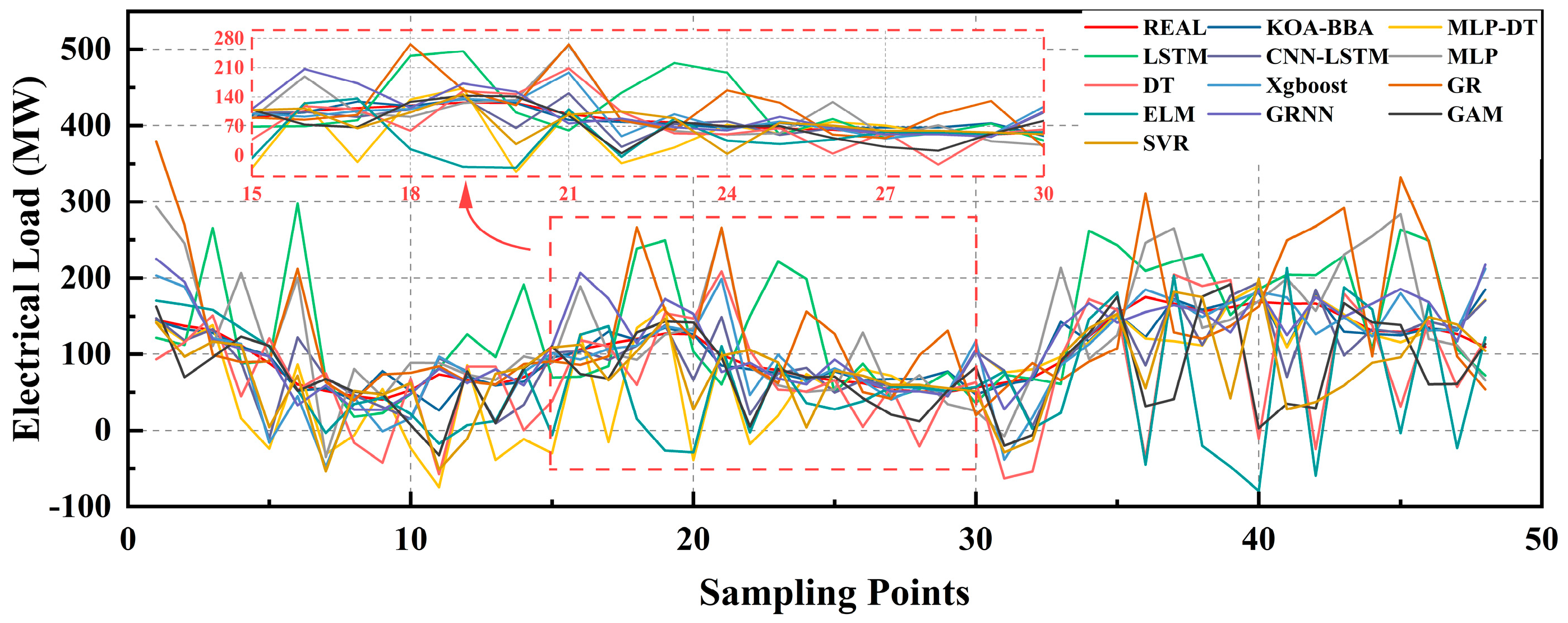
Figure 12.
Visualization of performance improvement.
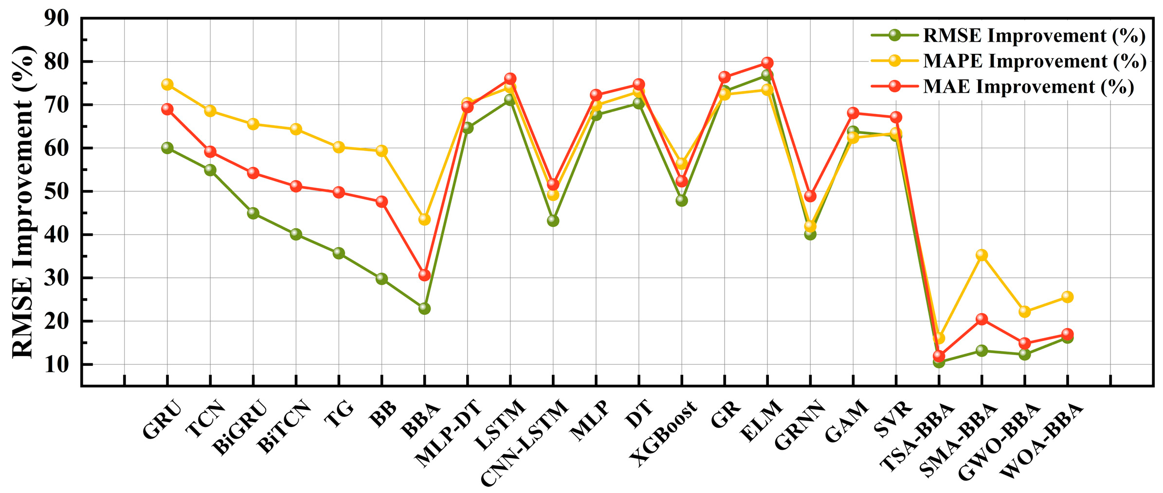

Table 1.
Number and type of missing values.
| Variables with missing values | Number of missing values |
|---|---|
| Power load | 128 |
| Relative humidity | 23 |
| Temperature (°C) | 15 |
| Direction of wind | 128 |
Table 2.
KNNI test performance.
| Model | RMSE | MAPE | MAE | R-squared |
|---|---|---|---|---|
| KNNI | 4.97 | 10.45 | 379.3 | 0.97 |
Table 3.
KOA Model parameters.
| Parameters | Values |
|---|---|
| Number of planets to search for | 20 |
| Maximum number of function evaluations | 5 |
| Range of Kernel sizes | [1,5] |
| Learning rate range | [0.001,0.01] |
| Range of neuron number | [100,130] |
Table 4.
BiTCN-BiGRU Model parameters.
| Parameters | Values |
|---|---|
| Number of planets to search for | 20 |
| Maximum number of function evaluations | 5 |
| Range of Kernel sizes | [1,5] |
| Learning rate range | [0.001,0.01] |
| Range of neuron number | [100,130] |
Table 5.
Performance comparison of ablation experiments.
| Model | RMSE | MAPE | MAE |
|---|---|---|---|
| GRU | 29.71 | 32.53 | 31.99 |
| TCN | 28.10 | 31.83 | 24.30 |
| BiGRU | 23.01 | 29.03 | 21.68 |
| BiTCN | 21.15 | 28.07 | 20.33 |
| TCN-GRU | 19.71 | 25.13 | 19.76 |
| BiTCN-BiGRU | 18.05 | 24.61 | 18.95 |
| BiTCN-BiGRU-Attention | 16.44 | 17.71 | 14.31 |
| KOA-BiTCN-BiGRU-Attention | 12.68 | 10.01 | 9.93 |
Table 6.
Performance comparison of different optimization algorithms.
| Model | RMSE | MAPE | MAE |
|---|---|---|---|
| KOA-BiTCN-BiGRU-Attention | 12.68 | 10.01 | 9.93 |
| TSA-BiTCN-BiGRU-Attention | 14.17 | 11.92 | 11.27 |
| SMA-BiTCN-BiGRU-Attention | 14.60 | 15.46 | 12.48 |
| GWO-BiTCN-BiGRU-Attention | 14.46 | 12.86 | 11.66 |
| WOA-BiTCN-BiGRU-Attention | 15.13 | 13.45 | 11.96 |
Table 7.
Classical algorithms predict comparative performance.
| Model | RMSE | MAE | MAPE |
|---|---|---|---|
| XGBoost | 20.86 | 17.14 | 20.08 |
| Gaussian Regression | 48.11 | 38.96 | 38.01 |
| ELM | 48.34 | 40.29 | 35.07 |
| GRNN | 20.95 | 16.95 | 19.63 |
| GAM | 30.57 | 25.53 | 25.38 |
| SVR | 29.40 | 25.03 | 27.17 |
| LSTM | 22.09 | 20.54 | 20.21 |
| KOA-BiTCN-BiGRU-Attention | 12.68 | 9.93 | 10.01 |
| MLP-DT | 29.34 | 24.04 | 27.58 |
| LSTM | 42.32 | 36.42 | 40.37 |
| CNN-LSTM | 21.55 | 17.55 | 19.18 |
Disclaimer/Publisher’s Note: The statements, opinions and data contained in all publications are solely those of the individual author(s) and contributor(s) and not of MDPI and/or the editor(s). MDPI and/or the editor(s) disclaim responsibility for any injury to people or property resulting from any ideas, methods, instructions or products referred to in the content. |
© 2024 by the authors. Licensee MDPI, Basel, Switzerland. This article is an open access article distributed under the terms and conditions of the Creative Commons Attribution (CC BY) license (http://creativecommons.org/licenses/by/4.0/).
Copyright: This open access article is published under a Creative Commons CC BY 4.0 license, which permit the free download, distribution, and reuse, provided that the author and preprint are cited in any reuse.


