
Submitted:
17 September 2025
Posted:
19 September 2025
You are already at the latest version
Abstract
We have investigated and theoretically developed a mathematical model that, first, allows us to understand how the positional exactitude of the output link of a four-bar mechanism depends on the manufacturing dimensional tolerances (associated with the IT grades, which correspond to the bilateral tolerances specified in the ISO 286-2 norm) of its links and the error of the input coordinate. To find this dependence, the total differentials of the kinematic constraint functions that govern the field of positions must be determined for each kinematic cycle of the mechanism under consideration. These total differentials lead to a system of equations whose solution gives the positional errors of the movable output links as a function of the manufacturing dimensional errors and an incidence matrix that varies with each one of the positions of the input element. On the other hand, the theoretical transmission ratio between the output velocities with respect to the input velocity of the articulated kinematic chain is defined, and for determining the total errors in each ratio, the total differential of each one of them is calculated, showing a clear dependence respect to the positional errors of the output links (previously defined) of the mechanism. The sum of the theoretical transmission ratio and its respective error provides the real transmission ratio. Furthermore, the described methodology allows determining the sensitivity (influence coefficients) in the transmission ratios due to errors inherent in the links lengths. Finally, the presented analytical approach is numerically implemented through an example of articulated parallelogram design, principally characterizing in graphic form the transmission ratios in their regions of permitted movements and blocking positions, for a specific IT degree of precision of the bilateral dimensional tolerances of their functional geometric parameters, with the objective of analyzing every aspect related to the performance of the mechanisms. The methods and conclusions proposed in this document also leave open the way as future work to study separately the magnitudes and signs of the positional errors and the transmission ratio, or even the influence coefficients themselves, in order to assign the most convenient degree of IT precision for each link in the mechanism with the purpose of reducing errors in the designs and obtain better efficiency in the transmission ratio.
Keywords:
4-bar mechanism
; dimensional tolerances
; influence coefficients
; transmission ratio
1. Introduction
The purpose of any mechanism composed of interconnected elements is to convert the energy supplied to the input link into force or movement toward the output link. Fundamentally, articulated mechanisms are used today in many practical industrial applications (machines) around the world, some of which require a high degree of positional exactitude of their output links around one or various prescribed operating positions that allow define the best possible efficiency in its transmission ratios.
During the past four decades, the world advanced manufacturing industry has been increasing its focus of attention on fabrication quality. It is common to observe that the drawings supplied by manufacturers do not provide, among other important technical specifications, manufacturing dimensional tolerances or clearances at kinematic linkage points, or the functional dimensions of the links, but rather a part number. This leaves unknown the role that manufacturing dimensional quality plays in the operation of an articulated mechanism, specifically the precision and movement requirements in the transmission ratios.
The analysis and synthesis of precision articulated mechanisms primarily require the challenge of achieving positional accuracy of the output element, making it vital to define the degree of precision of the dimensional tolerances of its components. Under common mechanical operating conditions, the manufacturing tolerances of the dimensional parameters of the kinematics chain are commonly assigned using the bilateral tolerances (IT grades) specified in the ISO 286-2:2010 norm.
The four-bar linkages, or “articulated quadrilaterals”, have a wide application in contemporary technology and great versatility and diffusion in the industry, also because this mechanism constitutes the most basic chain of links connected by rotating pairs that allow relative movement between the parts. Although these applications can be quite diverse, the four-bar linkages can be classified, depending on the tasks that they perform, as function generators, path generators, and motion generators [1, 2].
Historically, the knowledge necessary to elucidate the true importance of these aspects in the performance of the mechanism can be seen from the research of Sutherland et al. [3], in which they address the problem of designing a four-bar mechanism considering the errors introduced by the functional structure of the mechanism itself and by the dimensional tolerances in the path followed by a point of the coupler and in the positioning of the connecting rod. As a result of this work, a unique value of maximum dimensional tolerance is proposed that all the geometric parameters involved must have to guarantee the required accuracy. In 1995, Fogarasy et al. [4] developed a method in which, starting from the kinematic restriction equations and their total differentials, they calculate the velocities and accelerations for different cases of articulated plane mechanisms. However, to achieve this, they despise the errors that may be introduced by the generalized input coordinate. An extension work reported in [5] indicates the use of kinematic constraint equations to analyze the influence of the manufacturing tolerances in the kinematic performance of the mechanisms. The theme of the reliability of the real trajectory followed by a point of the coupler of an articulated mechanism when it must be generated with a specific precision, has generally been studied taking into account the influence of dimensional manufacturing errors and clearances existing in any deviation from the trajectory. For example, in [6] by assigning different IT degrees from an ideal distribution and by means of the Jacobian matrix method, the sensitivity of the dimensional tolerances respect to the quality of the performance in a four-bar linkage is determined, which allows to identify the most robust and ideal design. Other similar studies are implemented numerically for a slider-crank mechanism [7] and the kinematic synthesis of four-bar mechanisms for the generation of multiphase motion with tolerances [8]. As well, an analysis and synthesis procedure has been reported by Monte Carlo simulation that uses the measurement of the deviation of the real trajectory of the coupling point with respect to the desired one (reliability index), this method based on the reliability of the mechanical error in the trajectory generation mechanisms allows to assign optimal tolerances and clearances [9]. In the last decade, the use of specialized software in computational mechanics for modeling and simulation has allowed to optimize four-bar planar mechanisms from a dynamic and structural approach (considering external loads, displacement and vibration); this computational methodology can provide improved design data of stress, deformation and vibration frequency [10,11]. Furthermore, these software packages have contributed to developing optimized linkages by estimating the positional mechanical error of the output links as a function of the influence due to the sensitivities caused by the dimensions and tolerances of its components (pins, diameters of holes and lengths of links). In this regard, we can mention the error estimation through the numerical study of the modified partial derivative formulation [12], the deduction of the direct and inverse kinematics of the mechanism with respect to a set of variations in the tolerances and input coordinates to obtain the maximum error [13] and the use of a Taylor series approximation with modified error equation [14, 15]; all the previous reports were verified through a CAD model. Many researchers have addressed the optimization of dimensions and tolerances in mechanisms with the objective of satisfying the quality and minimizing the manufacturing costs of the manipulators, through various techniques such as Lagrange multipliers using an expanded formulation of the reciprocal power function cost-tolerance or genetic algorithm (see [16,17] and references therein).
Within the practical requirements of power transmission systems, it is important to maintain a constant ratio between the motions of the input link and its corresponding output element. To date, the analysis of specific cases of generating a quasi-constant transmission ratio [18-21] or the study of the quality of transmission angle ranges during the mechanism synthesis [22, 23] are topics that have been extensively investigated.
In the classical literature and scientific reports of the area, few are addressed regarding the influence or sensitivity in the transmission ratios of the output components due to dimensional errors or tolerances in the links lengths. An interesting study is reported in Ref. [24], where a robust design of mechanisms based on an analytical approach is proposed and flat four-bar and slider-crank articulated systems are analyzed for transmit the rotation between two parallel axes with a constant transmission ratio of 1:1. Here, the authors graphically illustrate the importance of reducing the transmission ratio sensitivity, product of the variations in the links length caused by the assignment of manufacturing tolerances or operating deformations, which highly affects the ideal theoretical value of the transmission ratio. And it is in this field of study where the main objectives of the work presented in this paper focus on establishing an analytical approach for 4-bar mechanisms that allows calculate independently the positional errors, the influence coefficients (sensitivities), the transmission ratios and their errors, as well as the ranges and regions of permitted and blocking motion, due to the assignment of dimensional tolerances by IT precision grades. This proposed formalism proves to be useful for analyzing the best efficiency in the transmission ratios and is another possible future option for defining admissible geometric variations.
The investigation presented in this document is organized as follows: The second section provides a complete overview of the theoretical foundations and mathematical procedures necessary for the deduction of explicit formulas to calculate the position errors/sensitivities and consequently the real positions of the output links. In that same sense, based on the derivations of the previous section, the third section delves into the analytical formalism for obtaining the errors/sensitivities in the transmission ratios and subsequently the real transmission ratios. The fourth section discusses the numerical implementation of the methodology, including graphical representations for a comparative analysis of the solutions for the ideal transmission ratios versus those dependent of the sensitivity due to bilateral tolerances/errors specified in ISO 286-2 norm (IT degrees) and the intervals of regions of permitted and blocking movement are characterized. Finally, the conclusions of the work are presented.
2. Mathematical Model to Evaluate the Influence of Dimensional Tolerances and Errors on Positioning Exactitude
In this section, we will develop a model that allows knowing the influences of the dimensional manufacturing tolerances of the geometric parameters and the angular deviation of the input link on the positioning error of the output links of a four-bar linkage mechanism. For this, the kinematic restriction equations of the mechanism will be found and its total differentials will be calculated. The results of the mathematical model that takes into account the influence of the dimensional tolerances of the geometric parameters allow us to know which of the functional dimensions of the mechanism links is the one that has the greatest or least influence on said positioning errors, thus being able to know which one link assign a greater or lesser degree of dimensional precision in order to guarantee a rigorous positioning of the output element in the case that the designer so requires.
The four-bar linkage mechanism can be considered like a mechanism with plane movement, the lengths of the links l1, l2, l3, l4 and their respective angles are represented in the Figure 1. It can be seen that both link l1 and link l3 are attached to the fixed frame by one of its ends. This mechanism is of one degree of freedom (demonstrated by the well-know Kutzbach–Gruebler equation) [25]. Therefore, knowing the lengths of the links a single input parameter is required to completely define their positions, this being the angle of the link l1, denoted as θ1.
The kinematic restriction equations obtained from the projection of the mechanism on the x and y axes are given by the equations (1) and (2), respectively:
The trigonometric scalar equations (1) and (2) can be solved simultaneously to find the output angles θ2 and θ3, defined as follows [25]:
Where
Equations (3) and (4) have two solutions, corresponding to the open and crossed configurations shown in the Figure 2.
2.1. Total Differentials of the Kinematic Constraint Equations and Positional Errors of the Output Links
Next, we will determine the total differential of the kinematic constraint functions that govern the field of positions. Such total differentials lead to a system of equations whose solution gives the positional errors of the mobile output links as a function of the manufacturing dimensional tolerances and of an incidence matrix that varies with each one of the positions of the input element.
Then, the total differential of the equations (1) and (2) with respect to the input and output coordinates (θ1, θ2 and θ3) and the geometric parameters (l1, l2, l3 and l4), is written as:
We are interested in obtaining the output positional errors, these errors are a function of the positioning error δθ1 of the input coordinate and the dimensional tolerances δl1, δl2, δl3 and δl4. Hence, we can express the total differentials indicated in the equations (5) and (6) in matrix form, through:
Thus, the output positional error vectors δθ2 and δθ3 are given by:
where
The product of both matrices forms the matrix , which contains the influence coefficients (), reducing the equation (8) as follows:
where
Each one of the terms of the matrix will be equal to:
In general, is the incidence matrix derived from the joint action of the errors in the input coordinate δθ1 and the manufacturing dimensional tolerances δl1, δl2, δl3 and δl4 of the geometric parameters of the mechanism. Notice that equation (9) can be obtained as long as the determinant of the equation (8) is different from zero. The null determinant of is obtained when , so we have the restriction ; with n∈Z. This only physically occurs in a special four-bar mechanism called “Articulated Parallelogram”, when the entry angle of the primary element is 0 or π, in which case all the links of the mechanism are aligned with each other [25].
Therefore, the complete calculation of the positioning errors for each one of the links 2 and 3 of a four-bar linkage mechanism is defined by rewriting equation (8) as:
It is important to indicate that the magnitudes of δl1, δl2, δl3 and δl4 depend on the values assigned by the international standards for Dimensional and Geometrical Product Specifications (GPS) and Verification, in particular the ISO 286-2:2010 standard (GPS — ISO code system for tolerances on linear sizes. Part 2: Tables of standard tolerance classes and limit deviations for holes and shafts) [26]. The use of this standard allows us to assign a tolerance range based on a nominal measurement (in mm), which corresponds to the functional geometric parameter lj of the mechanism. Twenty degrees (or indexes) of tolerance have been provided, designated by the abbreviations IT0, IT01 and IT1-IT18, from the most precise to the coarsest, whose numerical values are calculated for a group of nominal measurements and constitute the fundamental tolerances of the system. On the other hand, the positioning error δθ1 corresponding to the input angular coordinate only applies to elements that do not make complete turns, that is, for specific work positions. Its values are assigned according to the ISO 2768-1:1989 standard (General tolerances — Part 1: Tolerances for linear and angular dimensions without individual tolerance indications) [27].
Moreover, the coefficients ε21 to ε24 and ε31 to ε34 possess units of and have variable sign, which establishes the possibility that the designer controls the final sign of the product εijδlj, by assigning a fundamental position for the dimensional tolerance δlj (the ISO system defines 28 different positions with respect to the zero line as tolerance zones, see Upper and Lower limit deviations for shafts in [26]), in order to reduce the final output error around a specific operating position of the mechanism. The coefficients ε25 and ε35 are dimensionless.
Finally, the real position can be approximated by:
3. Transmission Ratio
The transmission ratio is defined as the output angular velocity divided by the input angular velocity of the mechanism. Below, we shall obtain the equations for the transmission ratio in a four-bar linkage mechanism, specifically we will find the transmission ratio between the input angle θ1 associated with the output angles θ2 and θ3.
The first step consists in isolate one of the two output angles in the left side of the equations (1) and (2), subsequently both sides of the equations are squared and added, finally is simplified by substitution of trigonometric identities. When carrying out this procedure for θ2 and θ3, the Freudenstein expressions are obtained [28,29]:
Further on, we implicitly derive the equations (15) and (16) with respect to θ1, namely:
As an outcome, we solve for the terms (i21) and (i31) that define the transmission ratios between the output and input angles, which are expressed by:
Obviously, the quotient of angular velocities is dimensionless.
3.1. Total Errors in the Transmission Ratio
As was shown in the previous section, it can be seen that the transmission ratio can be expressed as a function of the geometry and angular positioning of the links of the four-bar mechanism, therefore it is sensitive to positional errors and dimensional manufacturing tolerances.
In this section, we shall calculate the total differential of the equations (17) and (18) with respect to angular positioning and geometric parameters, in order to determine the total error in the transmission ratios, according to the next formulas:
where
If in the previous expressions we substitute the positioning errors δθ2 and δθ3, defined in the equations (11) and (12). The formulas (19) and (20) can be rewritten in function on the dimensional tolerances δl1, δl2, δl3, δl4 and δθ1 as:
where
According to the expressions (21) and (22), let us formally write the total errors of the transmission ratios i21 and i31 in matrix form, conveniently defined as:
Finally, the real transmission ratios can be approximated by:
4. Study cases
4.1. Parallelogram Four-Bar Linkage
Let us apply the derived formulas (17) and (18) for calculating the theoretical transmission ratios of a four-bar mechanism in parallelogram configuration (Special-Case Grashof linkage). The Grashof condition for a four-bar linkage is satisfied if S+L ≤ P+Q; where S is the shortest link, L is the longest, P and Q are the other links; this implies that at least one bar of the mechanism will be able to realize complete turns.
In this first case study, the nominal measurements of the elements (between hole centres) of the mechanism satisfy the conditions: l1=l3=25mm and l2=l4=250mm (S+L=P+Q). Specifically, we will present our results using the category of mechanism with change point, this category implies that during the movement in a determined position all the bars of the mechanism are collinear, therefore, the follower link can change its direction of rotation (two times per revolution of the input crank), see Figure 3. Consequently, the mechanism adopts the open configuration double-crank (the rotation angles of the cranks l1 and l3 are identical) and the crossed configuration crank-rocker. Notice that in the collinearity positions the movement of the mechanism becomes indeterminate and it can become an antiparallelogram mechanism, in practice the movement must be limited to avoid these positions.
The theoretical transmission ratios and are shown in the Figure 4, for open and crossed configuration. The results of our modeling show for the case of the transmission ratio (Figure 4a), that at the beginning of the movement from an open configuration (dotted blue line), that is, in the range 0°≤θ1≤π , the angles of rotation of the cranks l1 and l3 will be identical and consequently all the points of the connecting rod l2 will describe a semicircle of radius equal to the length of l1, which implies that both its angular displacement and velocity are zero, therefore = 0. Subsequently, in the position θ1=π, the four links are collinear and the mechanism undergoes the change point condition and begins the crossed configuration (antiparallelogram), in that second range (π ≤θ1≤2π) the cranks l1 and l3 rotate in opposite directions with unequal angular velocities, therefore, the link l2 experiences an increase in its angular displacement and hence acquires angular velocity, in that interval, the graph shows a inflection point and a curvilinear variation in the transmission ratio with a decay towards negative values which is due to the fact that when θ1≈275° the link l2 inverts the direction of rotation and its angular displacement begins to decrease until again all the links align (θ1=2π). Regarding the transmission ratio (Figure 4b), analyzing the solution in the range 0°≤ θ1≤π, when the movement of the mechanism begins from an open configuration (dotted blue line), as mentioned before, both the links l1 and l3 have the same angles of rotation and consequently the same angular velocities, this leads to =1. An inflection point is clearly observed in θ1=π, in which the articulated parallelogram switch to a crossed configuration, in the interval π ≤ θ1≤ 2π the cranks l1 y l3 rotate with unequal angular speeds and in the opposite direction, therefore the plot shows a descending curvilinear behavior with a negative solution (the minus sign indicates that the direction of rotation is inverted). The solid black line shown in the figures 4(a)-(b), indicates the transmission ratios and when the parallelogram four-bar initiates the movement from a crossed configuration and whose behavior obeys to the previous explanations.
On the other hand, we demonstrate the efficiency of the method proposed here, by comparing the transmission ratio with that calculated by the analytical approach through the Kutzbach–Gruebler equation described in Ref. [24]. The result obtained there, show good agreement whit our theory.
Besides, we also calculated the influence coefficients for the same parallelogram configuration. The Figure 5 exhibits the coefficients numerically-calculated and agree with the criteria for analyzing the sensitivities of the transmission ratio predicted by Rothenhofer et al. [24] (singularities exist at 0° and 180°). These coefficients, as well as the coefficients , are in function of the input angle and of each one of the lengths of the links, and can present positive or negative solutions in the open and crossed configuration ranges with a symmetrical behavior in both configurations, whose change point occurs at θ1=π. Their units are and determine the susceptibility in the calculation of the total errors of the transmission ratios and , for the case when the magnitudes of δl1, δl2, δl3, δl4 and δθ1 are not zero (see Eq. (23)).
4.2. Variations in the Link Lengths Due to Dimensional Tolerances
The most demonstrative case is the study of the real transmission ratios by solving numerically the equations (24) and (25). Within the formalism described in previous subsections and according to ISO 286-2:2010 standard, we can assign three qualities (amplitudes) of tolerances (e.g. IT01-ultraprecise, IT9-medium and IT18-very coarse) to the nominal measurement of the links of the mechanism. The Table 1 shows the amplitudes of the ISO tolerances for δl1, δl2, δl3 and δl4 as a function of the nominal measurements of the links (l1=l3=25mm and l2=l4=250mm). According to the Grashof law, in this type of mechanism the input angular coordinate ranges from 0 to 360 °, therefore its positioning error will be zero (δθ1=0).
We shall analyze the cases when the position of the tolerance zone with respect to the nominal measurement (Zero Line) is located above and below it (for practicality, the fundamental deviation criterion will not be considered). This means that the dimensional tolerances will be added or subtracted to the magnitude of the nominal measurements of the links (bilateral tolerances). To illustrate our results, in this section we present a comprehensive analysis of results for the particular case of the IT18 tolerance grade. Now, we should take into account that the articulated parallelogram mechanism in its theoretical design has only two different nominal measurements for its links, but considering the fact of adding or subtracting the tolerance, the final magnitude of the length of each link will have two variants. Therefore, sixteen different articulated four-bar mechanisms can be designed that are obtained from variations with repetition of two different measurements per link taken four at a time, that is 24 = 16 different designs. For a clearer idea, Table 2 shows the sign of the dimensional tolerances applied and type of Grashof condition for each articulated mechanism design.
The Figure 6 and Figure 7 show, respectively, the theoretical transmission ratios and in open configuration compared versus the real transmission ratios and , for Grashof mechanisms articulated parallelogram-type and of continuous motion with different degrees of tolerance. As it is seen, the figures 6(a)-(b) correspond to mechanisms that satisfy the condition S+L=P+Q and adjust to the discussion presented in section 4.1. Due to the change in the nominal measurements of the links, a change in the inclination of the slope is noticeable in the characteristic curves of the real transmission ratio with respect to the theoretical curve, both in the region of positive and negative values, being more pronounced in the case of designs when the dimensional tolerances increase the final size of the mechanism, note that all curves coincide in the change from positive to negative values at the same inflection point at θ1≈275°.
Now, in figures 7(a)-(b) a comparison is realized between the theoretical transmission ratios versus the real transmission ratios for two types of mechanism designs that depending on the dimensional tolerances applied to the nominal measurements, form the configuration Crank (l1)-Connecting rod (l2)-Rocker (l3), satisfying the condition S+L<P+Q. Based on the above, the graphs of the transmission ratios ideal theoretical and real do not show any similarity between them. The behavior of the curve for shown in Figure 7(a), makes evident the translation movement of the connecting rod, in the range of 0°≤θ1≤210° the slope shows a slight decrease, later from 210°≤θ1≤2π, the change in the inclination of the slope is pronounced, in addition two inflection points are observed for the change from positive to negative values at θ1≈95° and θ1≈275°. On the other hand, Figure 7(b) shows the curve for and it has a well-defined crest and trough behavior, demonstrating that this link does not have the capacity for complete rotation, this component connected to the base can only oscillate (rocker), there is an inflection point of change from positive to negative values at θ1≈π. As already mentioned in the previous section, for all the cases presented, the crossed configuration has a graphic mirrored- symmetrical behavior with respect to figures 6 and 7, whose explanation can be discussed in a similar way. Furthermore, the change from positive to negative values (or vice versa) in the evolution of the graphs indicates when the link invests its angular displacement.
Finally, the scope and utility of our analytical formalism extends to those linkages that do not have a continuous motion between them, known as non-Grashof mechanisms and satisfying the inequality S+L>P+Q. For our case of study, by modifying the nominal measurements of its components with the IT18 tolerance grade, ten mechanisms of this class are obtained. Since none of its three moving links realize a complete revolution with respect to the reference plane, they are always in oscillatory motion, this type of mechanisms are also called triple rocker. Therefore, one of the main objectives is to find out the interval of permissible limit positions of the input link.
Within this framework, the figures 8 and 9 illustrate, respectively, the real transmission ratios and , as well as the angular position range θ1 corresponding to the permitted movements. Additionally, they also provide the angular ranges of the blocking positions.
It is important to emphasize, that the behavior of the graphs must be carefully analyzed as follows: i) Here, we can identify vertical lines located on the horizontal axis at (or )=0 , when they intersect perpendicularly with those lines that coincide on this same axis (in some cases a slight deviation can be noticed due to precision errors in the numerical calculations), the value intervals of θ1 that define the blocking of the mechanism are specified, ii) On the other hand, we can notice that these same vertical lines can be directed towards positive or negative values ( as has been highlighted throughout this document, the above indicates the inversion of the direction of rotation of the link), and they are connected to each other end to end by means of a curve that indicates the transmission ratio of the angular interval of the allowed movement positions of the articulated assembly.
In what follows, for a better understanding of the analysis strategy indicated for the transmission ratios graphs illustrated in Figure 8 and Figure 9, Table 3 shows for the ten non-Grashof mechanism designs presented in this work, the ranges of the input angle θ1 for the allowed movements and the blocking of these articulated kinematic assemblies.
The results obtained demonstrate that the assignment of IT precision grades does not necessarily improve the performance of the mechanism. Some configurations satisfying the Grashoff condition deviate considerably from the ideal theoretical value of an articulated parallelogram. Furthermore, there are also cases where the increase of the bilateral tolerances leads to the Grashoff relation not being fulfilled. This complete characterization of the efficiency of the transmission ratios proposes the present methodology as a useful option for assigning the most appropriate IT precision grade for each nominal dimension of the links, with the purpose of reducing design errors and obtaining a better efficiency. Another notable feature of our approach lies in the separate calculation of the positional errors and transmission ratios, as well as the influence coefficients themselves.
5. Conclusions
The principal objective of this paper consisted in present an analytical and numerical methodology using the formulation of partial derivatives, for the estimation of real transmission ratios in 4-bar mechanisms, considering the influence of bilateral tolerances in the dimensions of their links. This formulation, as a first step, allowed us to predict for any angular position of the input element of the mechanism, the positional errors of the output links in function of the manufacturing tolerances of their functional dimensions and the positioning error of the input link itself. Subsequently, the errors of the transmission ratios were deduced, which demonstrated a dependence with the positional errors of the output elements, the sum of these errors with the theoretical ratio provided the real ratio of the mechanism. Our analytical approach allowed us to define an incidence matrix, formed by variable coefficients with the input coordinate that indicate the relative importance that has each geometric parameter of the mechanism in the positioning error at the output.
On the other hand, the numerical solution of the influence coefficients (relative influence that the dimensional tolerances have on the positioning error of the output links) and the theoretical transmission ratio , for an illustrative case of mechanism type articulated parallelogram, were validated through the analytical theory of Rothenhofer et al., where the only possible transmission ratio has a value of 1.
As mentioned in the previous sections, for common mechanical operating conditions, IT grades are used to assign bilateral tolerances to the dimensional parameters of a system, as specified in ISO 286-2 norm. Considering the same case study of articulated parallelogram, an IT18 tolerance grade was assigned. Our numerical calculations show that, as a result of the variations in the links lengths due to dimensional tolerances, when the articulated parallelogram condition is not met, the real transmission ratios of the mechanism deviate substantially from their ideal theoretical value (i.e. 1 for the case of ). It is even evident that such small changes in the lengths of its components in some cases cause unacceptable instantaneous variations in the transmission ratio (the Grashoff relation is no longer fulfilled).
It is important to highlight that the graphical representations of the real transmission ratios obtained by our approach allow us to characterize the efficiency of designs that meet the Grashoff condition, and beyond, define the permitted and blocking motion ranges for those designs that do not satisfy this condition. We can establish that we have a method that provides a complete overview for assigning a rational combination of dimensional tolerances for any degree of IT accuracy, with the goal of reducing the errors in the designs and achieving a better efficiency in the transmission ratio in 4-bar mechanisms.
To date, there are no reports in the classical and specialized literature in the area of synthesis and analysis of mechanisms that, unlike our theoretical formalism, provide expressions that independently calculate the errors in the transmission ratios and positional, as well as influence coefficients. Therefore, a future scope may lie in studying how the magnitudes and signs of the aforementioned parameters allow to assign the most appropriate IT precision degree for each nominal dimension, in order to obtain motion and precision conditions that translate into efficient transmission ratios.
Author Contributions
Conceptualization, J. Flores Méndez; Formal analysis, J. Flores Méndez, Gustavo M. Minquiz, A. Morales-Sánchez, Zaira Jocelyn Hernández Simón and A.C. Piñón Reyes; Funding acquisition, Luis Hernández Martínez; Investigation, J. Flores Méndez, José Alberto Luna López and A.C. Piñón Reyes; Methodology, J. Flores Méndez and Zaira Jocelyn Hernández Simón; Project administration, José Alberto Luna López, Luis Hernández Martínez and Nancy E. González Sierra; Resources, Gustavo M. Minquiz and Zaira Jocelyn Hernández Simón; Supervision, Zaira Jocelyn Hernández Simón, Luis Hernández Martínez and Nancy E. González Sierra; Validation, Gustavo M. Minquiz and Zaira Jocelyn Hernández Simón; Writing–original draft, J. Flores Méndez; Writing–review & editing, Gustavo M. Minquiz, A. Morales-Sánchez, Mario Moreno, Zaira Jocelyn Hernández Simón, José Alberto Luna López, Francisco Severiano Carrillo, Luis Hernández Martínez, Nancy E. González Sierra and A.C. Piñón Reyes. All authors have read and agreed to the published version of the manuscript.
Funding
This research received no external funding.
Institutional Review Board Statement
Not applicable.
Informed Consent Statement
Not applicable.
Data Availability Statement
Not applicable.
Acknowledgments
The authors would like to sincerely thank Tania Martínez Angel (Benemérita Universidad Autónoma de Puebla), due to his interest and dedication to the present research work, the results obtained were relevant for obtaining her title as an Engineer in Automation and Autotronics.
Conflicts of Interest
The authors declare no conflicts of interest.
References
- Katsumi Watanabe. Approximate Synthesis of Plane Four-Bar Mechanism for Curve Generation. Bulletin of the JSME 1975, 18, 536–544. [Google Scholar] [CrossRef]
- Katsumi Watanabe. Approximate Synthesis of Plane Four-Bar Mechanism for Function Generation. Bulletin of the JSME 1974, 17, 951–958. [Google Scholar] [CrossRef]
- G. H. Sutherland, N.R. Karwa. Ten-design-parameter 4-bar synthesis with tolerance considerations. Mechanism and Machine Theory 1978, 13, 311–327. [Google Scholar] [CrossRef]
- Fogarasy, M. R. Smith. The Case for a General Method of Kinematic Analysis of Plane Mechanisms Based on Equations of Constraint. Proceedings of the Institution of Mechanical Engineers - Part C. 1995, 209, 337–343. [Google Scholar]
- A. Fogarasy, M. R. Smith. The influence of manufacturing tolerances on the kinematic performance of mechanisms. Proceedings of the Institution of Mechanical Engineers, Part C. 1998, 212, 35–47. [Google Scholar]
- K. Ting, Y. Long. Performance Quality and Tolerance Sensitivity of Mechanisms. ASME. J. Mech. Des. 1996, 118, 144–150. [CrossRef]
- P. Flores, J. C. P. Claro. A Systematic and General Approach to Kinematic Position Errors Due to Manufacturing and Assemble Tolerances. Proceedings of the ASME 2007 International Design Engineering Technical Conferences and Computers and Information in Engineering Conference. Volume 5: 6th International Conference on Multibody Systems, Nonlinear Dynamics, and Control, Parts A, B, and C. Las Vegas, Nevada, USA. September 4–7, 43–49. ASME, 2007.
- R. S. Sodhi, K. Russell. Kinematic Synthesis of Planar Four-Bar Mechanisms for Multi-phase Motion Generation with Tolerances. Mechanics Based Design of Structures and Machines 2004, 32, 215–233. [Google Scholar] [CrossRef]
- Zhongxiu Shi, Fengqiang Li, Shian Qin, Fei Wang. Analysis and synthesis of mechanical error in path generating linkages based on reliability. Annual Reliability and Maintainability Symposium, Philadelphia, PA, USA, 303–306, 1997.
- Ruby Mishra, Gourishankar Mohapatro, Rojaline Behera. Structural and dynamic analysis of optimized four bar mechanism considering counterweight in coupler link. Materials Today: Proceedings 2018, 5, Part–1. [Google Scholar] [CrossRef]
- Ruby Mishra. Mechanisms of flexible four-bar linkages: A brief review. Materials Today: Proceedings 2021, 47, Part 16, 5570–5574. [Google Scholar] [CrossRef]
- H. P. Jawale, A. Jaiswal. Investigation of mechanical error in four-bar mechanism under the effects of link tolerance. J. Braz. Soc. Mech. Sci. Eng. 2018, 40, 383. [Google Scholar] [CrossRef]
- D. A. Dsouza, A. Jaiswal, H. P. Jawale. Positional Error Estimation of Five-Bar Mechanism Under the Influence of Tolerances. In: V. K. Gupta, C. Amarnath, P. Tandon, M. Z. Ansari (Eds). Recent Advances in Machines and Mechanisms. Lecture Notes in Mechanical Engineering, Springer, Singapore, 2023.
- Jaiswal, H. P. Jawale. Influence of tolerances on error estimation in P3R and 4R planar mechanisms. J. Braz. Soc. Mech. Sci. Eng. 2022, 44, 62. [Google Scholar] [CrossRef]
- Jaiswal, H. P. Jawale. Estimation of error in four-bar mechanism under dimensional deviations. Int. J. Interact. Des. Manuf. 2024, 18, 541–554. [Google Scholar] [CrossRef]
- Armillotta. Concurrent optimization of dimensions and tolerances on structures and mechanisms. Int. J. Adv. Manuf. Technol. 2020, 111, 3141–3157. [Google Scholar] [CrossRef]
- S. Velmurugan, K. Sivakumar, S. Ramabalan. Impact of mixed tolerance combination on the geometric position and torques of a four-bar kinematic chain using genetic algorithm. Materials Today: Proceedings 2022, 66, Part 3, 1056–1065. [Google Scholar]
- G. Figliolini, E. Pennestrì. Synthesis of Quasi-Constant Transmission Ratio Planar Linkages. ASME. J. Mech. Des. 2015, 137, 102301. [Google Scholar] [CrossRef]
- Kai Liu, Xianwen Kong, Jingjun Yu. Algebraic synthesis and input-output analysis of 1-DOF multi-loop linkages with a constant transmission ratio between two adjacent parallel, intersecting or skew axes. Mechanism and Machine Theory 2023, 190, 105467. [Google Scholar] [CrossRef]
- Kai Liu, Xianwen Kong, Jingjun Yu. Algebraic synthesis of single-loop 6R spatial mechanisms for constant velocity transmission between two adjacent parallel, intersecting or skew axes. Mechanism and Machine Theory 2024, 200, 105725. [Google Scholar] [CrossRef]
- K. Liu, J. Yu. Algebraic Method for Exact Synthesis of One-Degree-of-Freedom Linkages With Arbitrarily Prescribed Constant Velocity Ratios. ASME. J. Mech. Des. 2022, 144, 063301. [Google Scholar] [CrossRef]
- R. Karakuş, E. Tanık. Transmission angle in compliant four-bar mechanism. Int. J. Mech. Mater. Des. 2023, 19, 713–727. [Google Scholar] [CrossRef]
- Xiaoyong Wu, Qingping Liu, Jun Ding, Congzhe Wang, Haoyong Yu, Shaoping Bai. Transmission angle of planar four-bar linkages applicable for different input-output links subject to external loads. Mechanism and Machine Theory 2024, 203, 105829. [Google Scholar] [CrossRef]
- Gerald Rothenhofer, Conor Walsh, Alexander Slocum. Transmission ratio based analysis and robust design of mechanisms. Precision Engineering 2010, 34, 790–797. [Google Scholar] [CrossRef]
- Robert, L. Norton, Milton P. Higgins. Design of Machinery: An Introduction to the Synthesis and Analysis of Mechanisms and Machines. 6th edition, McGraw Hill, 2019.
- ISO 286-2:2010. Geometrical product specifications (GPS)-ISO code system for tolerances on linear sizes. Part 2: Tables of standard tolerance classes and limit deviations for holes and shafts. 2nd edition, 2010.
- ISO 2768-1:1989. General tolerances-Part 1: Tolerances for linear and angular dimensions without individual tolerance indications. 1st edition, 1989.
- F. Freudenstein. Design of Four-Link Mechanisms. Ph.D. Thesis, Columbia University, New York, USA, 1954.
- Ghosal. The Freudenstein equation. Resonance 2010, 15, 699–710. [Google Scholar] [CrossRef]
Figure 1.
Classic Four-bar linkage mechanism notation.
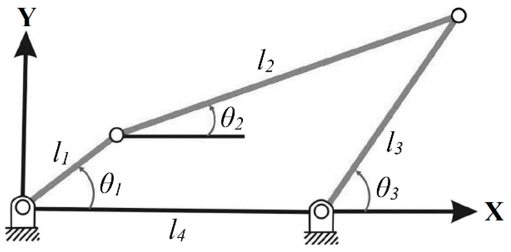
Figure 2.
Open and crossed configurations of the Four-bar linkage mechanism.
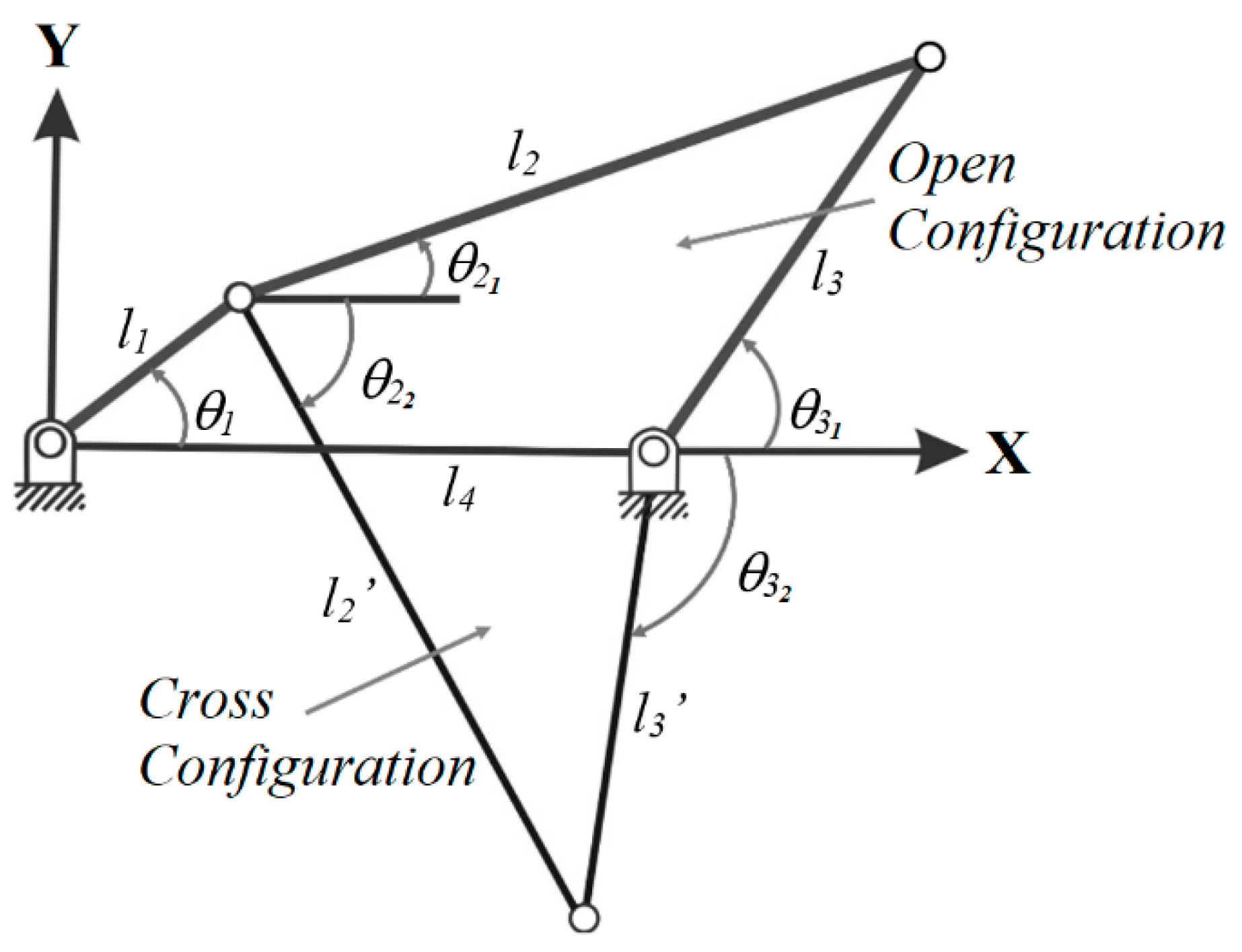
Figure 3.
Category of four-bar mechanism with change point (S+L=P+Q).
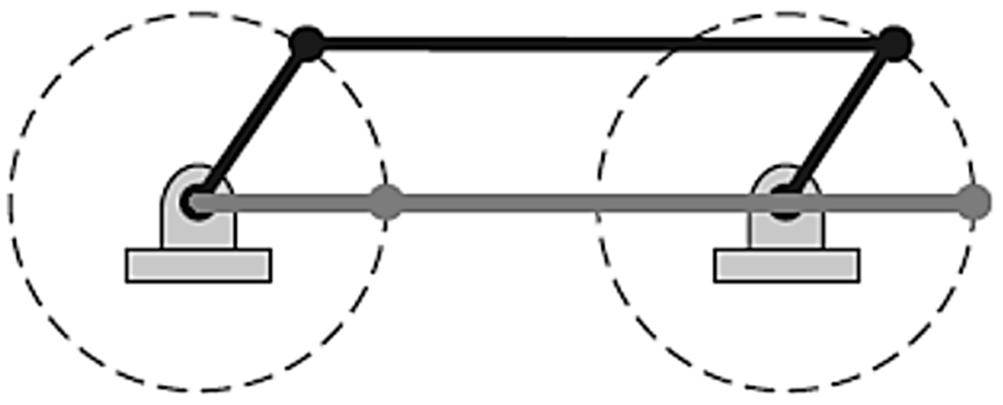
Figure 4.
Theoretical transmission ratios (a) and (b) in open and crossed configuration.
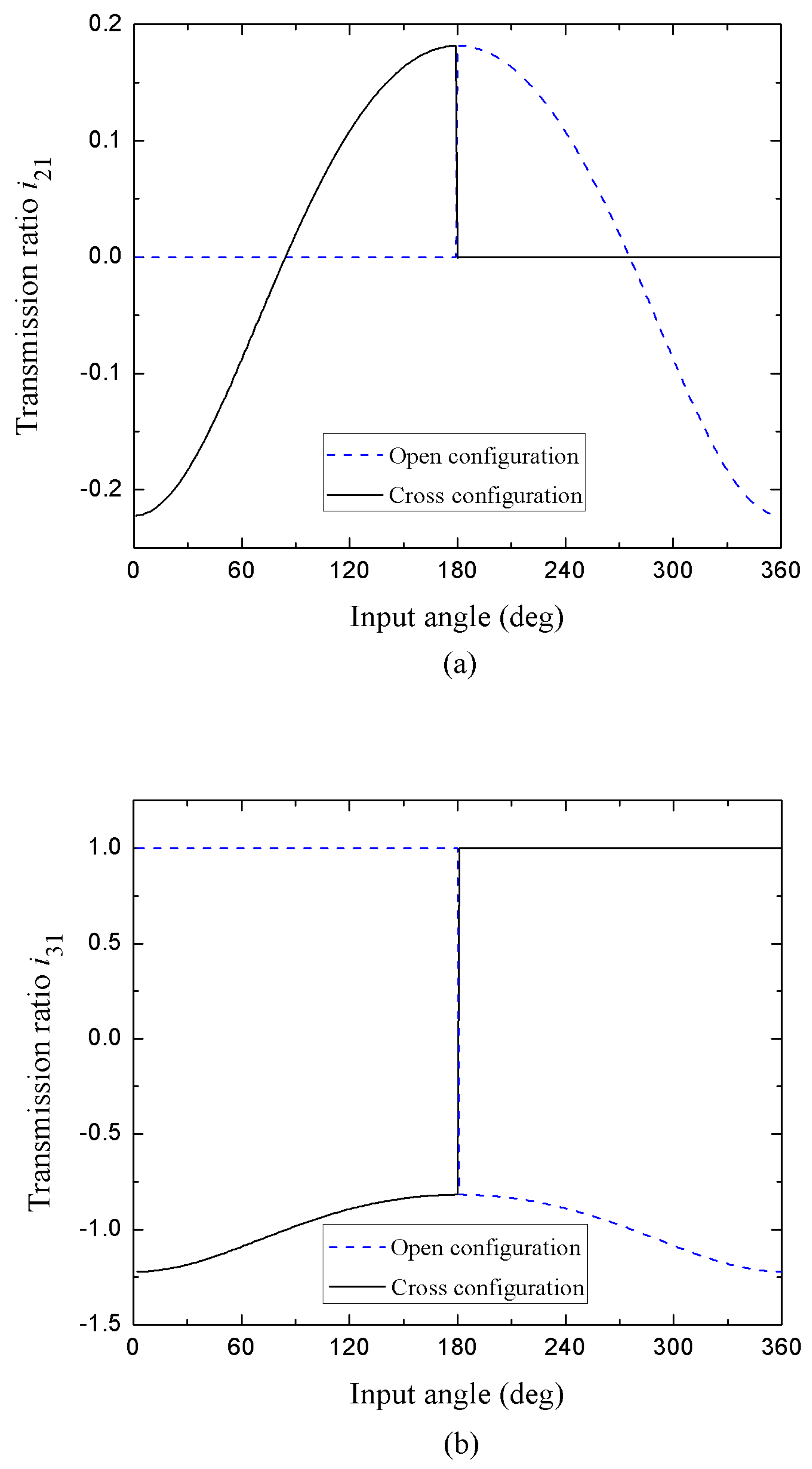
Figure 5.
Influence Coefficients (a), (b), (c) and (d).
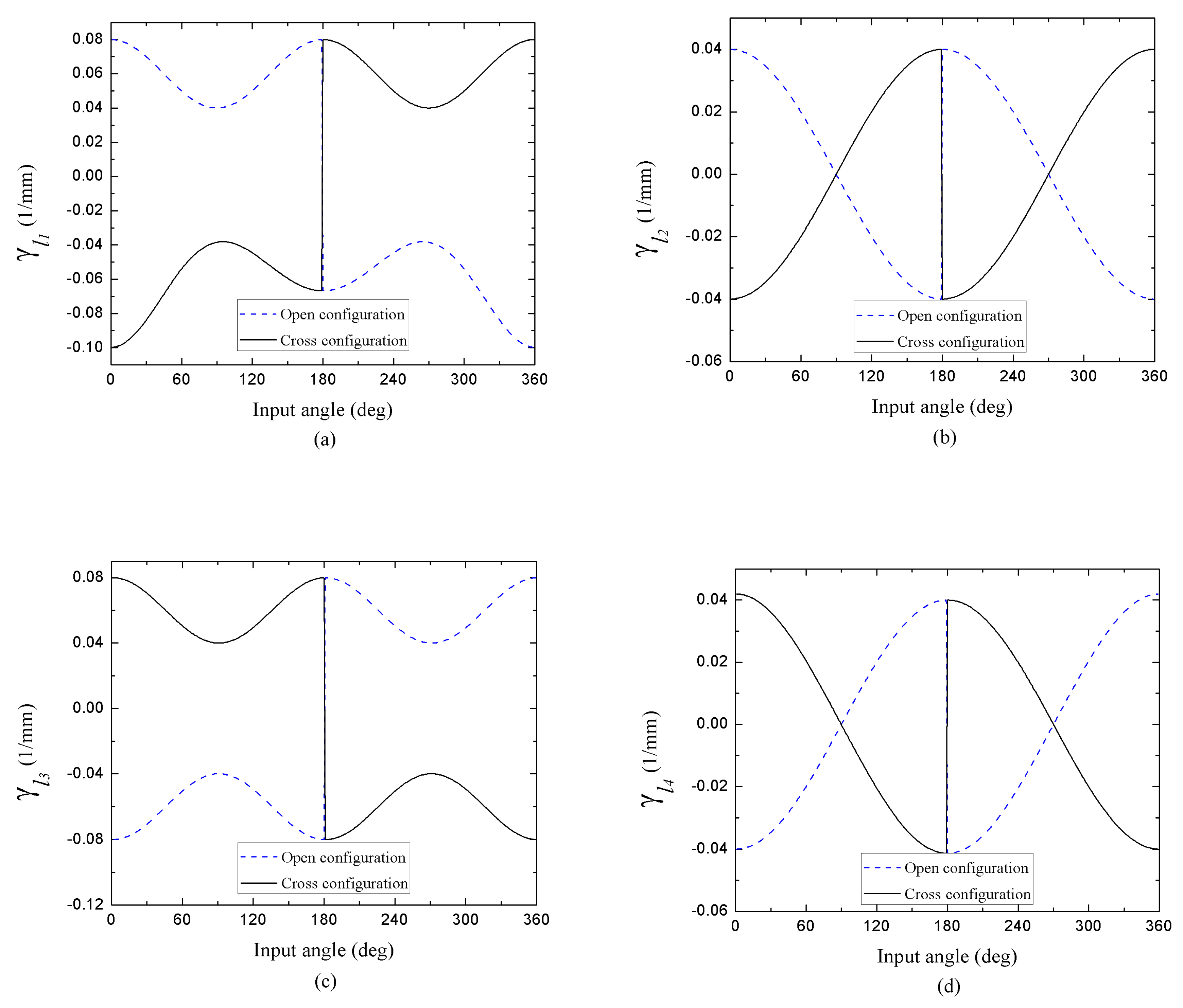
Figure 6.
Theoretical transmission ratios (a) and (b) in open configuration compared versus the real transmission ratios and of designs with dimensional tolerances that satisfy the condition S+L=P+Q (Grashof Mechanisms-Articulated Parallelogram).
Figure 6.
Theoretical transmission ratios (a) and (b) in open configuration compared versus the real transmission ratios and of designs with dimensional tolerances that satisfy the condition S+L=P+Q (Grashof Mechanisms-Articulated Parallelogram).
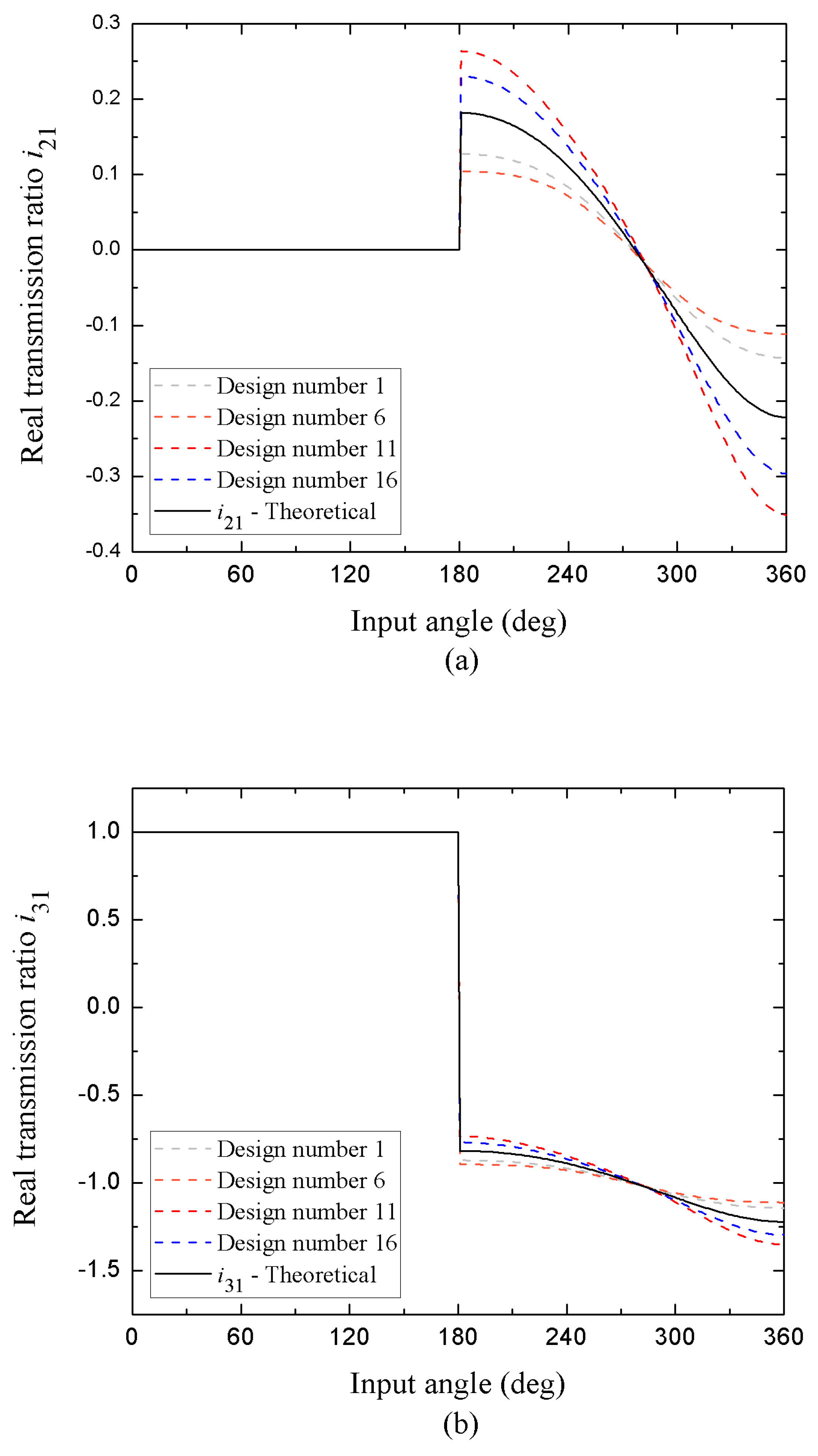
Figure 7.
Theoretical transmission ratios (a) and (b) in open configuration compared versus the real transmission ratios and of designs with dimensional tolerances that satisfy the condition S+L<P+Q (Grashof Mechanisms-Continuous Movement).
Figure 7.
Theoretical transmission ratios (a) and (b) in open configuration compared versus the real transmission ratios and of designs with dimensional tolerances that satisfy the condition S+L<P+Q (Grashof Mechanisms-Continuous Movement).
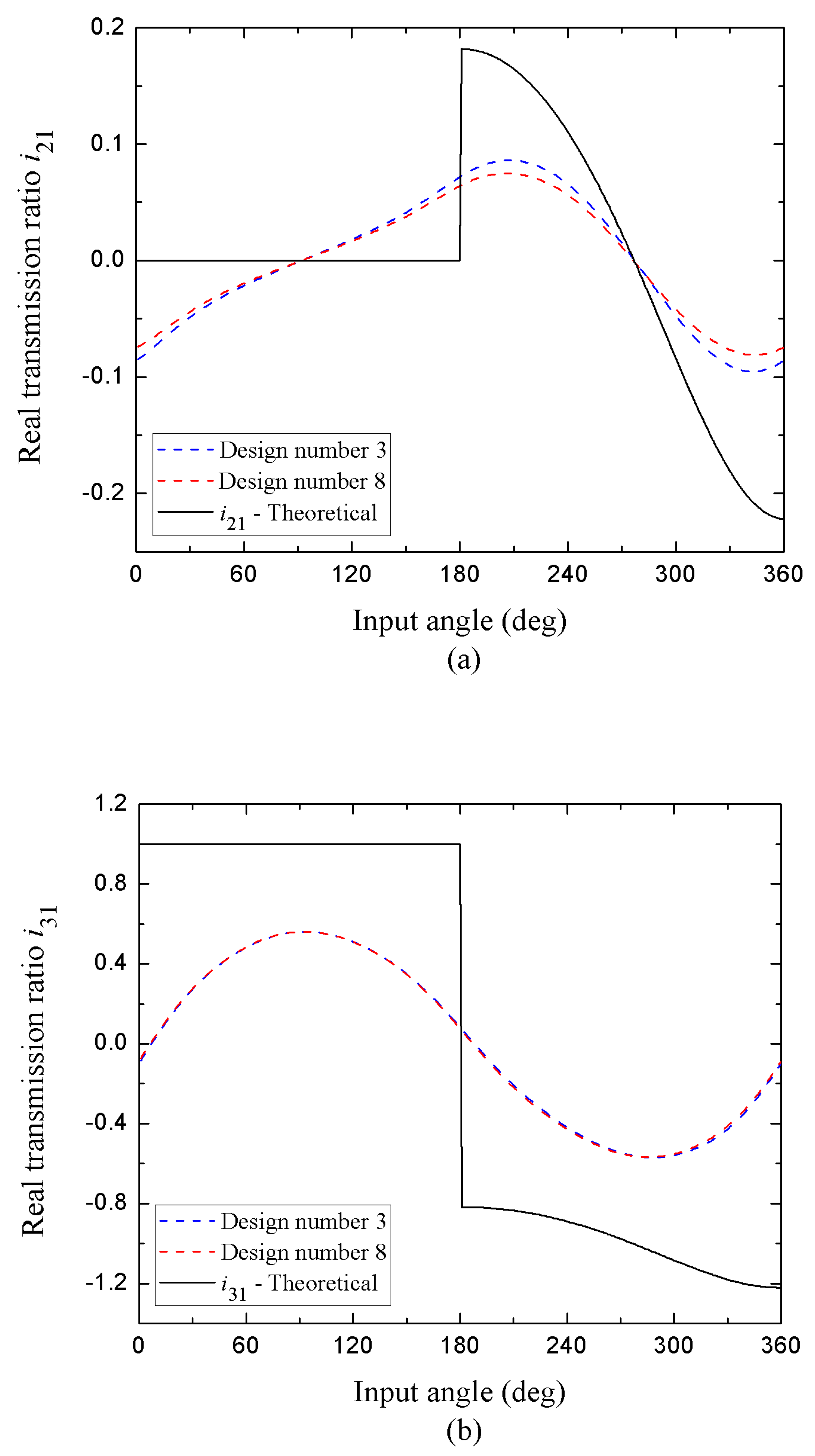
Figure 8.
Real transmission ratio (and angular position range) of the permitted movements and intervals of the locking positions of designs with dimensional tolerances that satisfy the condition S+L>P+Q (Non-Grashof mechanisms), see panels (a) and (b).
Figure 8.
Real transmission ratio (and angular position range) of the permitted movements and intervals of the locking positions of designs with dimensional tolerances that satisfy the condition S+L>P+Q (Non-Grashof mechanisms), see panels (a) and (b).
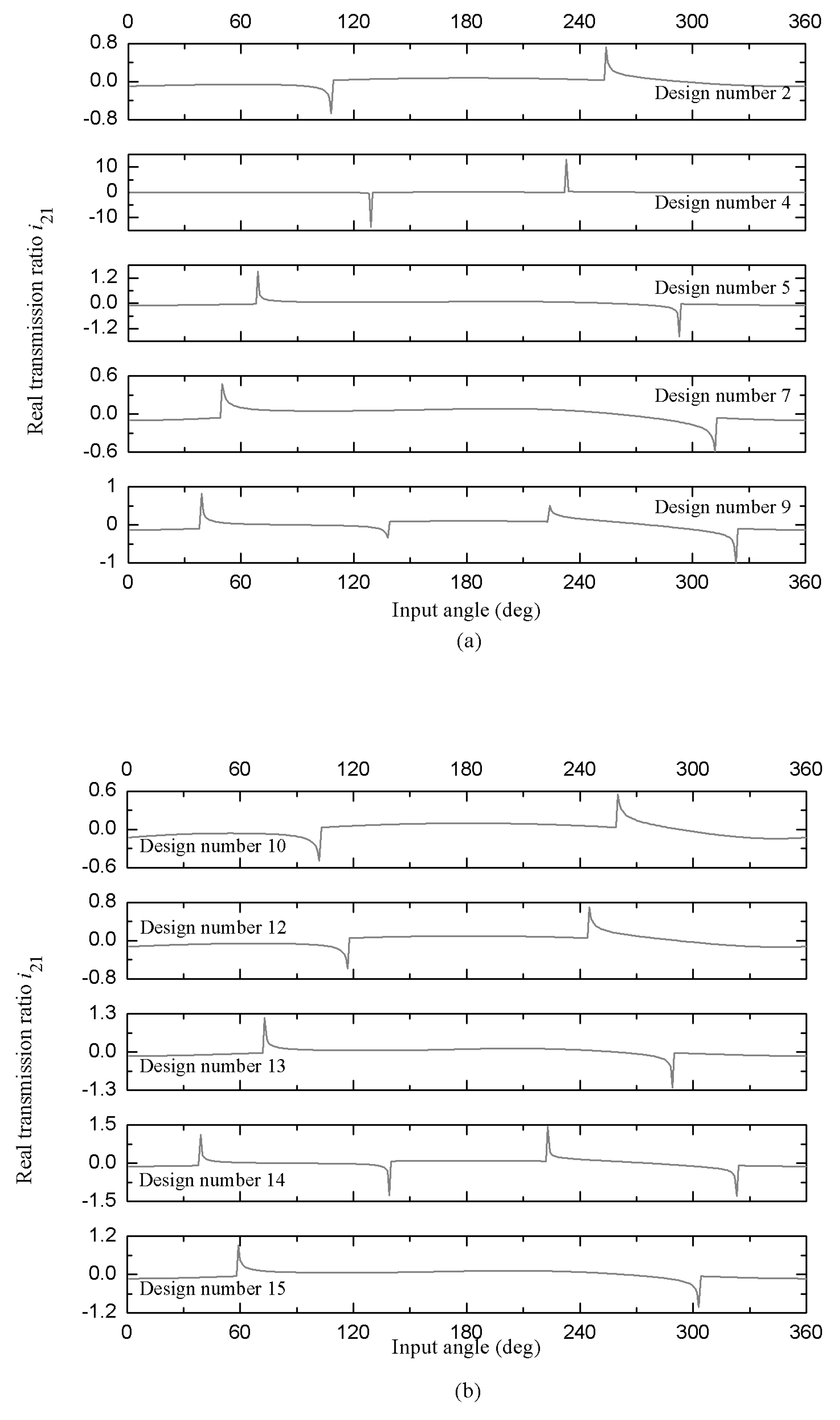
Figure 9.
Real transmission ratio (and angular position range) of the permitted movements and intervals of the locking positions of designs with dimensional tolerances that satisfy the condition S+L>P+Q (Non-Grashof mechanisms), see panels (a) and (b).
Figure 9.
Real transmission ratio (and angular position range) of the permitted movements and intervals of the locking positions of designs with dimensional tolerances that satisfy the condition S+L>P+Q (Non-Grashof mechanisms), see panels (a) and (b).
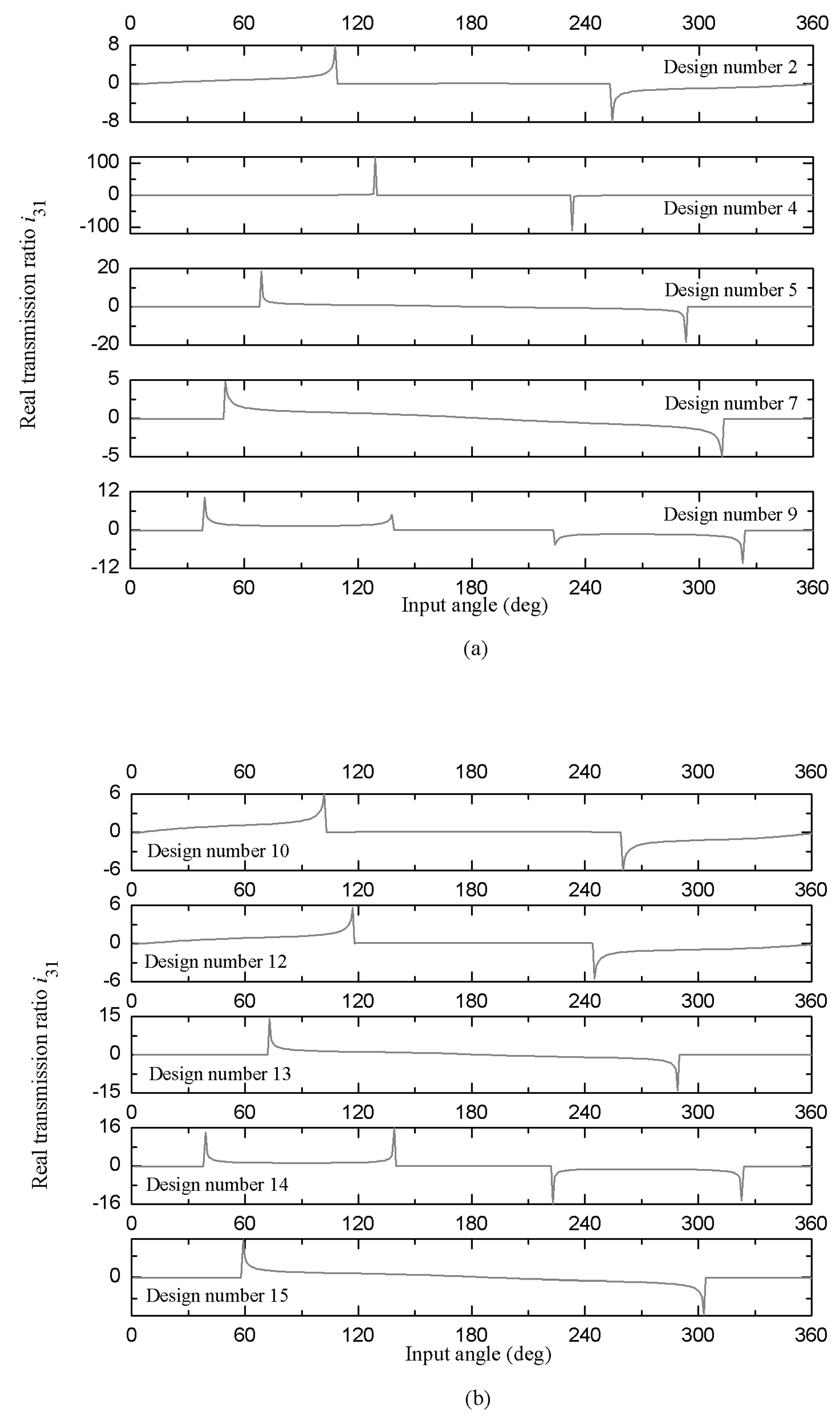

Table 1.
Dimensional tolerances depending on the nominal measurement of the links and the quality index.
Table 1.
Dimensional tolerances depending on the nominal measurement of the links and the quality index.
| Dimensional Tolerance | Quality (Grade) of Tolerance | ||
|---|---|---|---|
| IT01 (mm) | IT9 (mm) | IT18 (mm) | |
| δl1 | 0.0006 | 0.052 | 3.3 |
| δl2 | 0.002 | 0.115 | 7.2 |
| δl3 | 0.0006 | 0.052 | 3.3 |
| δl4 | 0.002 | 0.115 | 7.2 |
Table 2.
Sign of the dimensional tolerances and Grashof condition for the 16 designs of articulated mechanisms.
Table 2.
Sign of the dimensional tolerances and Grashof condition for the 16 designs of articulated mechanisms.
| Design number | Sign of Dimensional Tolerances | Grashof condition | ||||
|---|---|---|---|---|---|---|
| 1 | -δl1 | -δl2 | -δl3 | -δl4 | S+L=P+Q | |
| 2 | -δl1 | -δl2 | -δl3 | δl4 | Non-Grashof | |
| 3 | -δl1 | -δl2 | δl3 | -δl4 | S+L<P+Q | |
| 4 | -δl1 | -δl2 | δl3 | δl4 | Non-Grashof | |
| 5 | -δl1 | δl2 | -δl3 | -δl4 | Non-Grashof | |
| 6 | -δl1 | δl2 | -δl3 | δl4 | S+L=P+Q | |
| 7 | -δl1 | δl2 | δl3 | -δl4 | Non-Grashof | |
| 8 | -δl1 | δl2 | δl3 | δl4 | S+L<P+Q | |
| 9 | δl1 | -δl2 | -δl3 | -δl4 | Non-Grashof | |
| 10 | δl1 | -δl2 | -δl3 | δl4 | Non-Grashof | |
| 11 | δl1 | -δl2 | δl3 | -δl4 | S+L=P+Q | |
| 12 | δl1 | -δl2 | δl3 | δl4 | Non-Grashof | |
| 13 | δl1 | δl2 | -δl3 | -δl4 | Non-Grashof | |
| 14 | δl1 | δl2 | -δl3 | δl4 | Non-Grashof | |
| 15 | δl1 | δl2 | δl3 | -δl4 | Non-Grashof | |
| 16 | δl1 | δl2 | δl3 | δl4 | S+L=P+Q | |
Table 3.
Input angle intervals that define allowed movements and blocking positions.
| Design number | Input angle interval θ1 | |
|---|---|---|
| Allowed movements | Blocking positions | |
| 2 | 0≤θ1≤107° and 253°≤θ1≤360° | 108°≤θ1≤252° |
| 4 | 0°≤θ1≤128° and 232°≤θ1≤360° | 129°≤θ1≤231° |
| 5 | 68°≤θ1≤292° | 0°≤θ1≤67° and 293°≤θ1≤360° |
| 7 | 49°≤θ1≤311° | 0°≤θ1≤48° and 312°≤θ1≤360° |
| 9 | 38°≤θ1≤137° and 223°≤θ1≤322° | 0≤θ1≤37°,138°≤θ1≤222° and 323°≤θ1≤360° |
| 10 | 0≤θ1≤101° and 259°≤θ1≤360° | 102°≤θ1≤258° |
| 12 | 0≤θ1≤116° and 244°≤θ1≤360° | 117°≤θ1≤243° |
| 13 | 72°≤θ1≤288° | 0≤θ1≤71° and 289°≤θ1≤360° |
| 14 | 38°≤θ1≤138° and 222°≤θ1≤322° | 0°≤θ1≤37°, 139°≤θ1≤221° and 323°≤θ1≤360° |
| 15 | 58°≤θ1≤302° | 0°≤θ1≤57° and 303°≤θ1≤360° |
Disclaimer/Publisher’s Note: The statements, opinions and data contained in all publications are solely those of the individual author(s) and contributor(s) and not of MDPI and/or the editor(s). MDPI and/or the editor(s) disclaim responsibility for any injury to people or property resulting from any ideas, methods, instructions or products referred to in the content. |
© 2025 by the authors. Licensee MDPI, Basel, Switzerland. This article is an open access article distributed under the terms and conditions of the Creative Commons Attribution (CC BY) license (http://creativecommons.org/licenses/by/4.0/).
Copyright: This open access article is published under a Creative Commons CC BY 4.0 license, which permit the free download, distribution, and reuse, provided that the author and preprint are cited in any reuse.


