
Submitted:
06 October 2025
Posted:
08 October 2025
You are already at the latest version
Abstract
Hamstrings–quadriceps (H–Q) imbalance represents a biomechanical marker of knee instability and injury risk in running. This in silico study introduces a simulation-derived machine-learning framework designed to estimate H–Q imbalance using biomechanical features conceptually mappable to inertial-sensor domains. A reduced musculoskeletal framework emulating flexor–extensor balance, limb symmetry, and co-contraction patterns generated 573 synthetic running trials for 160 virtual subjects across three speeds. These interpretable features trained a calibrated gradient-boosting classifier evaluated via ROC-AUC, PR-AUC, balanced accuracy, F1, and Brier score. Across all conditions, the model achieved ROC-AUC 0.933 (95% CI 0.908–0.958), balanced accuracy 0.943, PR-AUC 0.918, F1 0.940, and Brier 0.056, outperforming a calibrated logistic baseline. Dynamic H:Q ratio and knee-moment symmetry were the dominant predictors, while co-contraction contributed complementary nuance. These results indicate that simulation-derived digital frameworks can reproduce IMU-relevant biomechanical variability, enabling interpretable machine learning for objective assessment of muscular balance in sports medicine.
Keywords:
inertial technologies
; interpretable machine learning
; hamstrings–quadriceps imbalance
; musculoskeletal simulation
; limb symmetry index
; co‐contraction index
; sports biomechanics
1. Introduction
The balance between hamstrings (H) and quadriceps (Q) is a fundamental determinant of knee joint stability, particularly during dynamic activities such as running. An altered H–Q relationship has long been implicated in heightened risk of anterior cruciate ligament injuries, hamstring strains, and reduced efficiency of locomotion [1,2,3]. Beyond injury prevention, the ability to monitor muscle balance dynamically is central for performance optimization and safe return-to-sport decision-making [4,5]. These factors underscore why H–Q imbalance remains a critical focus within sports biomechanics and rehabilitation.
Previous literature has extensively examined this imbalance. Epidemiological data confirm that hamstring injuries are the most frequent time-loss injury in elite sport and are characterized by high recurrence rates despite preventive programs [6,7,8]. Investigations into H:Q ratios demonstrate associations with both hamstring strain and ACL risk, though cut-off thresholds vary across tasks and protocols [9,10,11]. Limb symmetry indices (LSI) are routinely applied as clearance criteria in return-to-sport paradigms, yet several reports caution that they may overestimate recovery and fail to detect persistent neuromuscular deficits [12,13]. In parallel, machine learning methods have been explored in injury prediction, typically yielding moderate predictive accuracy and limited interpretability, raising concerns about their clinical utility [14,15,16]. Collectively, these findings highlight both the progress and the unresolved challenges in imbalance assessment, setting the stage for the present framework.
Despite its relevance, current assessment methods present significant limitations. Isokinetic and isometric dynamometry provide clinically standardized indices of H:Q strength but are inherently static and joint-isolated, offering limited ecological validity for dynamic running tasks [17]. Surface electromyography (EMG) and kinematic analyses extend insight into muscle activation and coordination, yet they are often sensitive to protocol design, instrumentation, and signal processing, leading to variability and limited reproducibility [18,19]. More recently, machine learning approaches have been applied to kinematic and kinetic datasets to classify injury risk and neuromuscular states. While such models achieve encouraging accuracy, they frequently operate as black boxes, providing predictions without interpretable links to underlying biomechanical mechanisms [20,21]. This lack of transparency creates a gap between computational performance and clinical or coaching applicability.
Controversy persists over how best to define and detect H–Q imbalance: some authors argue for universal dynamometric cut-offs [22,23,24], whereas others emphasize context-specific, task-dependent criteria [25,26,27]. Similarly, the promise of machine learning is tempered by debates regarding the balance between accuracy and interpretability, and whether opaque models can be trusted in applied sports science and medicine.
To address these challenges, biomechanical modeling provides a promising avenue. In this study, we adopt an inertial sensing paradigm implemented in silico via IMU-like signals—with “IMU” denoting the simulated sensor model, not a physical device. By reconstructing muscle-tendon dynamics, joint moments, and co-contraction patterns from motion data, simulation yields physics-informed features that retain explicit biomechanical meaning. In this framework, simulation-derived features such as dynamic H:Q ratios, knee-moment asymmetries, co-contraction indices, and timing variables are integrated into interpretable models to ensure both predictive robustness and biomechanical transparency. When combined with interpretable machine learning, this approach has the potential to bridge the gap, offering robust predictions while also providing transparent explanatory pathways.
Novelty of this study—most existing approaches are constrained by either static, isolated strength measures that do not reflect task specificity, or opaque machine learning models that lack biomechanical interpretability. Our work is, to our knowledge, the first in silico proof-of-concept that unites simulation-derived biomechanical features with interpretable machine learning for detecting H–Q imbalance in running. This dual contribution—physics-constrained features and transparent predictions—advances the methodological landscape and lays the foundation for translation to real datasets. Recent developments in wearable inertial measurement units (IMUs) enable field-based estimation of kinematic and dynamic quantities relevant to muscular balance. However, the translation of such signals into interpretable biomechanical markers remains limited. The present work bridges this gap by proposing a biomechanical modeling framework whose outputs are conceptually compatible with IMU-derived signals, supporting future sensor-based assessment of muscular balance.
Purpose and aim—the aim of this study is to demonstrate the feasibility of an in silico framework that leverages synthetic running data, simulation-derived features, and interpretable machine learning to detect H–Q imbalance. The principal conclusion anticipated is that such a framework can achieve robust classification while preserving biomechanical interpretability, thus providing a reproducible and transparent methodological baseline for future validation. The present work is not intended as clinical validation, but rather as a reproducible methodological demonstration, paving the way for future application on real datasets. Our objective is to deliver a transparent and interpretable digital framework—rather than to establish or revise clinical thresholds or to claim clinical validity. All reported results should therefore be read as reproducible evidence that physics-constrained features combined with calibrated, interpretable machine learning can recover biomechanically plausible patterns of hamstrings–quadriceps imbalance. External generalizability remains to be established on empirical datasets, which we outline as the next step in the translational pathway.
Operational definition of imbalance—in our proof-of-concept, the binary target is operationalized by clinically recognized cut-offs on dynamic H:Q (<0.60 or >1.20), knee-moment LSI (>±12%), and early-stance CCI (>0.58). Our contribution lies in calibrating and continuously ranking this composite rule, and in quantifying the added value of probabilistic models compared with fixed thresholds.
Based on the clinical importance of hamstrings–quadriceps balance and the methodological aims of this in silico study, we formulated the following hypotheses:
H1.
Hamstrings–quadriceps imbalance, defined by clinically recognized cut-offs (dynamic H:Q < 0.60 or > 1.20; knee-moment LSI > 12%), can be detected with high sensitivity and specificity using a digital in silico framework.
H2.
Dynamic H:Q ratio and knee-moment LSI will emerge as the dominant predictors of imbalance, confirming their central role in sports medicine for ACL risk assessment and return-to-sport clearance.
H3.
Explanatory analyses will reveal biomechanically plausible patterns—U-shaped effects for symmetry indices, monotonic effects for H:Q, and positive associations with co-contraction—ensuring that predictions reflect established neuromuscular mechanisms.
H4.
The framework will demonstrate stable performance across running speeds, reflecting its clinical utility in assessment protocols where intensity is varied to uncover hidden asymmetries.
H5.
Classification errors will concentrate near borderline clinical thresholds (e.g., H:Q ≈0.6–0.65; LSI ≈12–15%), reproducing the diagnostic uncertainty faced by clinicians in return-to-sport decisions.
H6.
Secondary predictors such as co-contraction index, stride-to-stride variability, and timing indices will provide complementary context for neuromuscular control, but will not outweigh the clinical importance of H:Q ratio and LSI.
2. Materials and Methods
The present work was designed as an in silico proof-of-concept study. Rather than relying on experimental motion capture data, we generated synthetic running datasets that emulate the biomechanical outputs typically derived from musculoskeletal simulations. This design allowed us to control variability, define imbalance conditions transparently, and test the feasibility of a digital assessment framework in a reproducible environment.
Hamstrings and quadriceps were chosen as the focal construct because their relative balance (H:Q ratio) is a well-established determinant of knee stability, anterior cruciate ligament (ACL) injury risk, and return-to-sport readiness. By centering the proof-of-concept on this clinically meaningful and biomechanically relevant problem, the proposed digital framework remains grounded in established sports medicine practice while simultaneously serving as a platform for methodological innovation.
Study design—the methodological workflow consisted of four main stages (Figure 1). First, Synthetic Data Generation, in which a population of virtual subjects and running trials was simulated across multiple speed conditions. Second, Simulation-Derived Feature Set, where dynamic H:Q ratios, limb symmetry indices, co-contraction metrics, and timing variables were derived. Third, Model Training and Validation, where machine-learning models were trained and evaluated under strict subject-wise validation, with calibrated probabilities and bootstrap confidence intervals. Finally, Interpretability and Reporting, where permutation importance, partial dependence, confusion matrices, error analyses, calibration, and reproducibility safeguards ensured that classification outputs could be traced back to biomechanical determinants. The overall workflow is summarized in Figure 1.
This staged structure was not merely procedural but designed to align synthetic data generation with biomechanical feature definition, statistical rigor, and interpretability, thereby ensuring that subsequent analyses rest on a framework that is both reproducible and physiologically meaningful.
In practice, the framework was implemented through a cross-sectional, in silico design that decoupled methodological evaluation from the heterogeneity of empirical motion-capture pipelines. Instead of analyzing human recordings, we synthesized running trials that emulate the principal outputs of musculoskeletal simulations—joint kinetics, loading symmetry, and co-contraction—across multiple speed conditions and repeated trials per individual. The unit of analysis was the virtual subject, with multiple simulated trials per subject; reporting follows the journal’s standards for methodological transparency and reproducibility.
The target construct was operationalized as a binary imbalance label derived from task-specific, dynamic criteria intended to reflect knee mechanics during stance rather than static strength alone. Labels were assigned using composite thresholds (dynamic H:Q ratio < 0.60 or > 1.20; |knee-moment LSI| > 12%; early-stance co-contraction index > 0.58), with a small fraction of stochastic flips to mimic real-world misclassification.
Predictors comprised a simulation-derived feature set chosen for biomechanical interpretability and coverage of complementary mechanisms: dynamic H:Q, limb-symmetry indices for knee moment, stance time and vertical GRF, early-stance co-contraction, temporal coordination (time-to-peak knee flexion moment), stride-to-stride variability (coefficients of variation), and running speed as a covariate. These definitions preserve an explicit link between the statistical model and the underlying physics of knee function during running.
To ensure subject-independent inference and calibrated decision support, all learning and evaluation procedures respected subject grouping (subject-wise GroupKFold, k = 5), probabilistic calibration (isotonic regression), and uncertainty quantification via bootstrap resampling of out-of-fold predictions on the primary metrics (ROC-AUC, PR-AUC, balanced accuracy, F1, Brier).
Taken together, this staged design aligns a controllable data-generating process with physics-constrained predictors and statistically rigorous validation, thereby grounding subsequent analyses in a framework that is simultaneously reproducible and physiologically meaningful.
2.1. Synthetic Data Generation
The first stage of the framework consisted of synthetic data generation, designed to emulate the structure and variability of athletic cohorts in a controlled digital environment. Although no physical inertial sensors were used, the modeled segmental dynamics were structured to emulate IMU-level signal characteristics, ensuring translational compatibility with wearable-sensor data. This step combined virtual subjects with simulated running trials, introduced variability across three speed bands, and applied clinically anchored labeling rules based on H:Qdyn, LSI, and CCI. Together, these components define a digital cohort representative of athletic variability and imbalance patterns.
Virtual Subjects—a virtual cohort of 160 synthetic subjects was constructed to emulate the neuromuscular diversity of an athletic population. Each subject was assigned a latent imbalance propensity, sampled from a bimodal Gaussian distribution, creating two subpopulations representing balanced and imbalanced neuromechanical profiles. The decision to model imbalance at the subject level—rather than at the individual trial level—ensured that the virtual cohort reflected how real athletes are studied in biomechanics and sports medicine, where the participant remains the primary unit of analysis. This choice aligns the framework with clinical research practice, where repeated measurements are used to characterize the neuromuscular profile of each athlete rather than being treated as independent observations.
Methodological and Clinical Relevance—subject-level design was further justified by the clinical importance of hamstrings–quadriceps (H:Q) imbalance in sports medicine. Prior studies have shown that H:Q ratios below ~0.6 or above ~1.2, together with limb asymmetries exceeding 10–15%, are predictive of heightened anterior cruciate ligament (ACL) injury risk and delayed return-to-sport clearance. By embedding these thresholds as latent parameters within each synthetic subject, the virtual cohort mirrored the decision criteria applied in rehabilitation and performance testing. This construction allowed the framework not only to simulate data but also to reflect the conceptual structure of clinical assessments, where imbalance is diagnosed per athlete, not per isolated trial.
Trials and Task Conditions—for each subject, between two and five running trials were simulated across three task intensities: slow (≈2.8 m·s−1), moderate (≈3.4 m·s−1), and fast (≈4.2 m·s−1). These speeds were chosen to correspond to experimental protocols in running biomechanics, where moderate velocities (~3 m·s−1) are typically used for baseline testing, and higher velocities (>4 m·s−1) reveal compensatory mechanisms that may not be apparent at lower intensities. A total of 573 trials were generated, producing a dataset large enough to evaluate model generalizability while maintaining subject-level coherence. Multiple trials per subject also captured intra-individual variability, reproducing the reality of repeated gait cycles in experimental and clinical contexts.
Variability and Realism—inter-individual heterogeneity was introduced by varying the latent imbalance parameters across subjects, thereby representing population-level diversity. Within each trial, stride-to-stride variability was modeled by perturbing biomechanical outputs, reflecting natural fluctuations in ground reaction forces, knee joint moments, and muscle activations. In addition, ~5% of labels were randomly flipped to simulate measurement errors and misclassification, which are common in empirical biomechanics due to sensor noise, marker placement variability, and EMG cross-talk. These design elements ensured that the synthetic dataset preserved not only structure but also the imperfections of real-world cohorts, avoiding the misleading stability of purely deterministic models.
Ethical and Methodological Advantages—the use of virtual subjects offered methodological advantages that extend beyond convenience. It allowed systematic manipulation of imbalance prevalence and severity without ethical risks associated with overloading real athletes. It also enabled precise control over confounding variables, such as trial intensity and noise level, which are difficult to isolate in empirical settings. Moreover, the digital cohort facilitated full reproducibility, since every subject could be regenerated under the same probabilistic rules, an advantage rarely achievable in clinical research where recruitment and data collection are subject to variability and attrition.
Taken together, the construction of the virtual cohort provided a physiologically plausible and methodologically transparent foundation for the in silico study. By grounding imbalance at the subject level, embedding variability at multiple scales, and aligning parameters with thresholds widely discussed in sports medicine, the framework ensured that subsequent analyses retained direct muscular meaning. This approach positioned the synthetic cohort not as a statistical abstraction but as a controlled analogue of real athletes, in which hamstrings–quadriceps balance could be studied with rigor, reproducibility, and translational relevance.
Key design parameters of the virtual cohort, together with their methodological rationale and quantitative implementation, are summarized in Table 1.
As shown in Table 1, the virtual cohort was not defined merely by arbitrary numerical choices but by explicit links to clinical and biomechanical constructs. Subject-level imbalance was embedded through bimodal latent distributions, repeated trials captured intra-individual variability, and controlled label noise mimicked empirical measurement error. Moreover, threshold definitions for H:Q, LSI, and CCI directly shaped class prevalence, providing a transparent connection between digital rules and clinical decision criteria. These elements collectively ensured that the synthetic dataset retained both structural realism and interpretability.
Key distributional parameters of the generator were as follows: latent imbalance propensity was sampled from a bimodal Gaussian distribution (balanced cluster μ=0.5, σ=0.10; imbalanced cluster μ=1.5, σ=0.10). Dynamic H:Q values were perturbed with Gaussian noise (σ=0.05), while stride-to-stride variability was implemented with a coefficient of variation of ≈5%. Knee-moment LSI and CCI were mapped from the latent imbalance propensity with thresholds set at ±12% and 0.58, respectively, with Gaussian perturbations σ=0.03. Running speeds were centered at 2.8, 3.4, and 4.2 m·s−1 (σ=0.10). Random label flips of ≈5% were applied uniformly across trials to mimic empirical misclassification. The random seed was fixed at 2025 to ensure reproducibility across all analyses.
Taken together, the construction of the virtual subjects provided a physiologically plausible and methodologically rigorous foundation, ensuring that subsequent running trials and labeling procedures remained anchored in hamstring–quadriceps physiology.
Running Trials—to complement subject-level design, each virtual individual was modeled through repeated running trials across multiple task intensities, ensuring that imbalance was expressed under dynamic and variable biomechanical conditions.
Trial design across three speed—each virtual subject was simulated to perform between two and five running trials, spanning three standardized speed bands: slow (~2.8 m·s−1), moderate (~3.4 m·s−1), and fast (~4.2 m·s−1). These velocities were selected to reflect commonly adopted benchmarks in gait and sports biomechanics, where moderate speeds provide baseline neuromuscular assessment, and higher speeds elicit compensatory strategies that are often associated with elevated injury risk. The design yielded a total of 573 trials, distributed evenly across the three conditions, thereby ensuring statistical balance while maintaining subject-level variability.
Biomechanical relevance of running speed—speed modulation is known to influence joint loading, muscle activation dynamics, and neuromechanical control strategies. At lower running speeds, joint kinetics are more symmetrical and less demanding, whereas faster speeds amplify asymmetries and challenge the hamstrings–quadriceps balance by increasing extensor torque requirements and co-contraction demands. Embedding this range of velocities into the virtual cohort ensured that imbalance was evaluated not under static or idealized conditions, but across ecologically valid task intensities that replicate the challenges of sports performance.
Intra-trial stride-to-stride variability—to further enhance realism, stride-to-stride variability was introduced within each trial. Rather than producing identical repetitions, synthetic cycles were perturbed by adding small fluctuations to ground reaction forces, joint moments, and timing of muscle activation patterns. This design decision reflects empirical findings in gait biomechanics, where even trained athletes exhibit cycle-to-cycle variability due to neuromuscular noise, motor unit recruitment variability, and external perturbations. By embedding intra-trial fluctuations, the simulated trials captured the stochastic nature of human movement and prevented the unrealistic stability characteristic of purely deterministic models.
Methodological and clinical significance—the inclusion of both speed variation and stride variability served not only to increase dataset diversity but also to reinforce clinical and methodological relevance. In experimental biomechanics, repeated trials across different speeds are a cornerstone of return-to-sport assessment, as they expose hidden asymmetries and neuromuscular deficits that may not be evident under controlled, low-intensity tasks. By integrating these principles into the in silico framework, the virtual running trials provided a physiologically grounded substrate from which biomechanical features could be extracted, ensuring that subsequent analyses retained direct muscular and clinical meaning.
Taken together, the structure of repeated running trials across different speeds, enriched with stride-to-stride variability, provided a realistic experimental substrate for generating biomechanical features and defining imbalance in a clinically meaningful manner.
Labeling Strategy—to transform raw simulations into clinically interpretable outcomes, each trial was assigned a class label based on established biomechanical thresholds, thereby defining balanced versus imbalanced conditions.
Thresholds and biomechanical rationale—labels were assigned according to three core constructs: the dynamic hamstrings–quadriceps ratio (H:Qdyn), the knee-moment limb symmetry index (LSI), and the co-contraction index (CCI) during early stance. Thresholds were set at H:Qdyn <0.6 or >1.2, LSI >10–15%, and elevated CCI beyond the expected physiological range, reflecting benchmarks commonly cited in sports medicine. These cut-offs were selected because they correspond to return-to-sport clearance criteria and predictors of anterior cruciate ligament (ACL) injury risk, thereby anchoring the labeling system in clinically recognized definitions of imbalance.
Integration into the synthetic framework—the thresholding rules were embedded directly into the synthetic cohort at the subject level, ensuring that each virtual athlete was consistently classified across trials. For instance, a subject with systematically low H:Qdyn values would be designated imbalanced across all trials, while stride-level fluctuations around the threshold could still produce trial-to-trial variability. This approach reflected how athletes are clinically categorized: as balanced or imbalanced individuals, even though variability is inherent in repeated performance assessments.
Sensitivity to cut-offs and prevalence shifts—because imbalance prevalence depends on threshold selection, systematic sensitivity analyses were conducted. Shifting the LSI cut-off from 10% to 15% reduced imbalance prevalence by ~1.8%, while a −0.05 adjustment to the H:Qdyn threshold increased prevalence by ~2.1%. Overall, prevalence varied within ±2–3% across reasonable threshold ranges. These controlled shifts ensured that labeling was both realistic and transparent, demonstrating that clinical decision rules inherently carry uncertainty that propagates into classification outcomes.
Noise and realism—to mimic the imperfections of empirical datasets, approximately 5% of labels were randomly flipped. This procedure simulated the effect of marker placement errors, EMG cross-talk, and inter-rater variability, all of which are common sources of misclassification in biomechanics research. This procedure not only introduced realistic uncertainty but also slightly altered the overall class prevalence, typically by ±2–3% compared with the nominal 288 vs. 285 design. Such minor shifts mirror the effect of measurement noise in biomechanics, where empirical prevalence estimates often vary depending on threshold definitions and evaluator error. By integrating label noise, the framework avoided presenting artificially perfect data and instead reproduced the ambiguity characteristic of clinical assessments.
Taken together, the labeling strategy anchored imbalance detection in clinically validated thresholds while acknowledging the variability and uncertainty inherent to empirical practice, thereby reinforcing the physiological credibility of the synthetic cohort.
In this way, the synthetic cohort established the conditions from which biomechanical features could be systematically extracted and analyzed.
Linking Dynamic H:Q to Clinical Cut-offs—conventional hamstrings–to–quadriceps (H:Q) thresholds (e.g., <0.60 or >1.20) originate primarily from isokinetic dynamometry, which reflects isolated strength under static or joint-controlled conditions. In this proof-of-concept, these values were therefore used as clinical anchors rather than as literal transfer values. The imbalance definition operationalized here is based on a dynamic H:Q index (H:Qdyn_{dyn}dyn) that integrates flexor–extensor moments over the stance phase, thereby providing a task-specific reflection of knee loading during running. This design preserves the link with familiar clinical scales while recognizing that dynamic ratios may differ quantitatively from static measures.
To ensure that conclusions do not hinge on any single numerical choice, we performed pre-specified sensitivity analyses by shifting H:Qdyn_{dyn}dyn cut-offs by ±0.05 and varying the knee-moment LSI threshold between 10% and 15%. These perturbations altered class prevalence by only ≈2–3% and confirmed that discrimination and calibration remained stable across plausible definitions. Thus, the framework should be interpreted as anchored to clinically recognized thresholds, yet robust to their exact placement, reinforcing its validity as a methodological baseline for imbalance detection.
Transparency of the generator—to ensure reproducibility, the virtual cohort and trial structure were generated using explicit formulas and parameter values reported in the cohort design tables of Section 4.1. All stochastic elements, including Gaussian perturbations and ≈5% label flips, were controlled by a fixed random seed (seed = 2025), ensuring that the dataset can be regenerated identically from the specifications provided. This design emphasizes transparency: imbalance labels are not arbitrary, but derived from clinically anchored thresholds (H:Qdyn_{dyn}dyn < 0.60 or > 1.20; |LSI| > 12%; CCI > 0.58), with controlled variability and misclassification noise to mimic empirical practice.
2.2. Simulation-Derived Feature Set
Each simulated running trial was characterized by a comprehensive set of simulation-derived biomechanical features designed to capture different aspects of knee joint function, symmetry, and neuromuscular control. The choice of features was motivated by their widespread use in biomechanics and clinical practice for assessing muscle balance, joint stability, and injury risk. To operationalize these constructs within the simulated dataset, we defined a set of features that translate biomechanical principles into quantitative indices, each capturing a distinct yet complementary facet of knee mechanics and neuromuscular function.
Dynamic Hamstrings-to-Quadriceps Ratio (H:Qdyn)—the H:Q ratio is a cornerstone metric for evaluating the balance between knee flexors (hamstrings) and extensors (quadriceps). Unlike static or isokinetic measures, the dynamic version integrates moments over the stance phase, providing a task-specific index of relative contribution:
where ∫ denotes an integral (a continuous sum across time), Mflex(t) and Mext(t) are the knee flexor and extensor moments, while dt indicates summation over infinitesimal time incrementsand. The interval tFS, tTO corresponds to the stance phase (from foot-strike to toe-off). This measure reflects the total effort of hamstrings relative to quadriceps. To avoid numerical instability when extensor moments approached zero, the denominator was stabilized with ε = 0.01.
Conceptually, H:Qdyn values below ~0.6 indicate disproportionate quadriceps dominance, whereas values above ~1.2 reflect hamstring over-dominance. Both extremes have been repeatedly associated with anterior cruciate ligament (ACL) injury risk and with delayed return-to-sport clearance, making H:Qdyn a clinically meaningful indicator of neuromuscular imbalance.
Limb Symmetry Index (LSI)—LSI is a widely used metric in biomechanics and sports medicine to quantify inter-limb asymmetry. It expresses the relative difference between the dominant and non-dominant limb, normalized as a percentage:
where Xdom and Xnondom represent peak values of the same feature (e.g., knee moment, stance time, or vertical GRF) from the dominant and non-dominant limb. An LSI of 0% indicates perfect symmetry; positive values indicate dominance of the stronger limb, while negative values favor the weaker limb. Dominant vs. non-dominant limb assignment was fixed at the subject level across all trials to ensure consistency of sign and interpretation.
Moderate asymmetries are expected in human movement, but values exceeding ±10–15% are commonly regarded as clinically relevant. High LSI values may reflect unilateral weakness, incomplete rehabilitation, or compensatory strategies that can increase injury risk.
Co-Contraction Index (CCI, Early Stance)—the CCI quantifies the degree of simultaneous activation of hamstrings (H) and quadriceps (Q), reflecting how much the two muscle groups co-activate to stabilize the knee during loading. It is computed at each instant of time and then averaged over early stance:
where, AH(t) and AQ(t) denote the time-varying normalized activations (or synthetic force proxies) of hamstrings and quadriceps. The numerator uses the smaller of the two values at each time point, ensuring that only the overlapping activation is counted. The denominator normalizes by the total activation of both muscle groups. As a result, CCI(t) ranges between 0 (no overlap) and 1 (perfect co-activation). The second formula computes the average CCI across the duration of early stance, where TES is the time length of that phase. Synthetic activations were normalized to a 0–1 scale before computation, and the index was averaged across the first 25% of stance to reflect early-loading stabilization.
A moderate level of co-contraction is beneficial for knee stability, especially after foot-strike when external loads are high. However, excessively high CCI values may indicate inefficient movement strategies, increased joint compression, and reduced energy efficiency, whereas very low values may compromise joint stability.
In addition to H:Qdyn, LSI, and CCI, supplementary features were derived to capture temporal and external load characteristics. These included the time to peak knee flexion moment (TTP-KFM), reflecting the timing of flexor demand relative to stance, and the vertical ground reaction force limb symmetry index (vGRF LSI), which quantified external load asymmetry between limbs. Both indices provided complementary information on joint loading strategies and neuromechanical control.
Time-to-Peak Knee Flexion Moment (TTP-KFM)—this feature represents the temporal coordination of knee joint loading. It is defined as the percentage of the gait cycle from foot-strike to the occurrence of maximum knee flexion moment:
where tpeak is the time of maximum knee flexion moment, tFS is the foot-strike event, and tcycle is the full gait cycle duration. The result is expressed as a percentage of the cycle. Foot-strike and toe-off were detected from vertical GRF > 20 N, and time-to-peak was expressed as a percentage of stance duration.
A delayed or premature time-to-peak may reflect altered neuromuscular strategies, compensatory patterns after injury, or fatigue-induced timing shifts.
Vertical GRF Peak LSI—Ground reaction force (GRF) symmetry reflects external loading balance between limbs. It was quantified using the same LSI formula as for joint moments:
where, Fdom and Fnondom are the peak vertical GRFs measured (or simulated) for the dominant and non-dominant limb.
Higher asymmetry in vGRF peaks can indicate unilateral weakness, residual deficits after injury, or compensatory strategies that shift loading away from the weaker limb.
Stride-to-stride irregularities were quantified using the coefficient of variation (CV), applied to selected biomechanical outputs. Low CV values indicated stable and consistent performance, whereas higher CV reflected instability, compensatory adjustments, or neuromuscular fatigue. This ensured that the feature set remained sensitive to both static thresholds and dynamic variability.
Variability Metrics (Coefficient of Variation, CV)—stride-to-stride variability is a measure of movement consistency. Increased variability often reflects instability, fatigue, or insufficient neuromuscular control. The coefficient of variation was applied to selected features such as dynamic H:Q ratios and LSI indices:
where, σ is the standard deviation and μ is the mean of the feature across multiple strides. The result indicates relative variability as a percentage.
Low CV values indicate consistent motor patterns and good control, while high CV values suggest instability, irregular loading, or compensatory strategies.
Finally, running speed was included as a contextual covariate to account for velocity-dependent differences in kinetics and coordination. Although not a clinical indicator per se, speed provided an essential control variable to ensure comparability across trials and conditions.
Contextual Variable (Running Speed)—running speed (vvv, in m·s−1) was included as a continuous covariate. Speed is known to strongly affect joint moments, GRFs, and timing variables. By including speed as a predictor, we controlled for velocity-dependent differences in biomechanics:
where d is the running distance and t is the time.
Including running speed as a contextual covariate allowed us to account for velocity-dependent changes in kinetics and coordination, ensuring that the derived features were comparable across trials performed at different intensities.
Taken together, the feature set captured complementary aspects of hamstrings–quadriceps balance, limb symmetry, co-contraction, and variability, ensuring that subsequent model predictions remained anchored in biomechanical constructs rather than abstract numerical patterns. To facilitate clarity and reproducibility, all simulation-derived biomechanical features are summarized in Table 2, together with their defining equations, labeling thresholds, and biomechanical interpretations. These features were then used as inputs for model training and validation, forming the next stage of the framework.
The summary provided in Table 2 highlights how each simulation-derived feature was explicitly grounded in biomechanical theory and linked to clinically recognized thresholds. By combining indices of muscle balance, inter-limb symmetry, co-contraction, temporal coordination, and variability, the framework captures complementary aspects of knee joint function. This integration ensures that model predictions are not abstract outputs but remain directly interpretable within established clinical paradigms of injury risk, rehabilitation, and return-to-sport decision-making. In this way, the feature set constitutes a physiologically meaningful foundation for the subsequent machine-learning analyses.
2.3. Model Training and Validation
The third stage of the framework consisted of model training and validation, which implemented the digital assessment pipeline through calibrated machine-learning procedures. This stage combined the generation of synthetic labels, the extraction of muscle-relevant features, and the training of Gradient Boosting classifiers with isotonic calibration. Validation was conducted using subject-wise cross-validation and bootstrap resampling, ensuring that performance estimates remained robust, transparent, and directly interpretable in biomechanical terms. In this way, the framework recast hamstrings–quadriceps imbalance into a form that could be systematically analyzed and evaluated.
2.3.1. Computational Model and Data Generator
The synthetic data generator was implemented as a computational module designed to instantiate virtual subjects, simulate running trials, embed variability across speeds and strides, and assign class labels based on biomechanical thresholds. This modular pipeline served as the technical engine of the framework, translating methodological assumptions into reproducible digital data streams.
Computational Model—the computational framework was designed to emulate the principal outputs of musculoskeletal simulations without implementing a full forward-dynamics solver. Rather than estimating forces and moments from experimental kinematics, we constructed a reduced but physiologically meaningful model that generates synthetic quantities aligned with established biomechanical concepts. Hamstrings–quadriceps interaction was not represented as isolated strength values but was operationalized dynamically through flexor–extensor moment balance, co-contraction indices, and symmetry metrics This approach ensured full control of variability, transparent labeling of imbalance conditions, and reproducibility of methodological steps.
The model rests on three fundamental assumptions. First, knee joint stability during running can be approximated through a small set of surrogate variables: flexor–extensor moment balance, inter-limb symmetry indices, ground reaction forces, and co-contraction patterns. Second, neuromuscular control can be represented using synthetic proxies for hamstrings and quadriceps activations, sufficient to compute indices of co-activation and timing. Third, subject heterogeneity can be mimicked through latent parameters sampled from controlled distributions, with additional random fluctuations introduced to approximate stride-to-stride variability and measurement noise.
Each virtual subject was represented by an underlying imbalance propensity parameter drawn from a bimodal Gaussian distribution, reflecting the dichotomy between balanced and imbalanced neuromechanical profiles commonly reported in running populations. Synthetic features—including dynamic hamstrings-to-quadriceps ratio, knee-moment limb symmetry index (LSI), stance-time LSI, vertical GRF LSI, co-contraction index (CCI), and time-to-peak knee flexion moment—were then derived as functions of this latent parameter with added Gaussian noise. This ensured that the generated data retained biomechanical plausibility while allowing for precise control over imbalance prevalence and feature variability.
A summary of the model components, their implementation, and rationale is provided in Table 3, consolidating the computational assumptions that guided the generation of synthetic trials.
As shown in Table 3, the computational set-up not only specifies how synthetic features were generated, but also clarifies their role in class labeling, expected influence on classification performance, and interpretability dimension. This level of transparency ensures that methodological decisions are explicitly linked to biomechanical constructs rather than treated as abstract modeling choices.
In summary, the computational model provided a controlled and physiologically grounded framework in which imbalance could be represented transparently through a small set of interpretable variables. By combining biomechanical plausibility with methodological flexibility, the set-up established a reproducible foundation on which subsequent stages of data generation and analysis were built.
Synthetic Data Generation—synthetic running trials were generated to emulate the biomechanical outputs typically obtained from musculoskeletal simulations while retaining full control over variability, balance between classes, and reproducibility. A virtual cohort of 160 subjects was created, each contributing between two and five trials across three speed conditions representative of natural locomotor demands: slow (~2.8 m·s−1), moderate (~3.4 m·s−1), and fast (~4.2 m·s−1). In total, 573 trials were produced, providing sufficient heterogeneity for model training and evaluation.
To embed inter-individual variation, each subject was assigned a latent imbalance propensity parameter sampled from a bimodal Gaussian distribution. This construct reflected the dichotomy between balanced and imbalanced neuromechanical profiles commonly observed in athletic populations. From these latent values, synthetic biomechanical features were derived, including dynamic H:Q ratio, knee-moment LSI, stance-time LSI, vertical GRF LSI, co-contraction index (CCI), and time-to-peak knee flexion moment. Gaussian noise was added to each feature to approximate both measurement error and stride-to-stride variability, ensuring stochastic variability consistent with empirical datasets.
Class labels were assigned using a composite rule grounded in biomechanical plausibility. A trial was classified as imbalanced if any of the following conditions were exceeded: dynamic H:Q ratio < 0.60 or > 1.20; |knee-moment LSI| > 12%; or early-stance CCI > 0.58. These thresholds align with values reported in sports medicine, where H:Q cut-offs are frequently debated as indicators of muscle imbalance, LSI deviations above 10–15% are considered clinically meaningful, and elevated co-contraction indices have been associated with compensatory or inefficient stabilization strategies. To mimic the imperfect ground truth typical of real assessments, ~5% of labels were stochastically flipped. This deliberate injection of label noise acted as a stress test for classifier robustness and prevented overfitting to idealized conditions.
The composite rules used to assign imbalance labels are summarized in Table 4, which consolidates the thresholds, biomechanical rationale, and methodological impact of each criterion.
By integrating latent subject parameters, stochastic perturbations, and clinically grounded thresholds, the synthetic dataset established a reproducible and physiologically coherent environment for evaluating the proposed framework. Beyond methodological demonstration, this design serves as a translational blueprint, ensuring that insights derived from simulation can be extended and validated on empirical running datasets in applied sports medicine contexts.
On this computational basis, the next step involved configuring and validating machine-learning classifiers trained on the generated biomechanical features.
2.3.2. Machine Learning Configuration, Validation Strategy, and Interpretability Procedures.
The machine learning component of the framework was designed to combine predictive accuracy with methodological transparency. Gradient Boosting was selected as the primary classifier given its balance of flexibility and interpretability, while a calibrated logistic regression served as a linear baseline for benchmarking. Probability estimates were calibrated using isotonic regression, ensuring that outputs could be interpreted as meaningful risk estimates rather than arbitrary scores. Validation was carried out at the subject level using a GroupKFold design, preventing data leakage across trials and ensuring independence between training and evaluation.
The classification framework was implemented using Gradient Boosting, a decision tree–based ensemble algorithm that constructs models sequentially to minimize prediction error. Gradient Boosting was selected because it offers a balance between predictive performance and interpretability: unlike deep neural networks or other black-box models, its structure allows for transparent feature importance analyses and partial dependence visualizations. As a benchmark, a calibrated logistic regression model was also implemented to provide a linear baseline against which to contrast the performance of the non-linear ensemble.
To reduce the risk of overfitting while retaining sufficient flexibility, the base learners were restricted to shallow decision trees with a maximum depth of three. Shallow trees constrain the number of interaction terms captured by each base learner, ensuring that the resulting ensemble remains both stable and interpretable. This choice reflects a deliberate compromise: deeper trees could increase raw predictive accuracy at the expense of interpretability, whereas overly shallow learners (depth one or two) risk discarding meaningful biomechanical interactions.
All probability estimates were calibrated using isotonic regression. Calibration was prioritized because in applied biomechanics and sports medicine, probabilistic outputs should reflect the empirical likelihood of imbalance rather than arbitrary scores. Among available calibration techniques, isotonic regression was chosen over Platt scaling because it does not assume linearity in the log-odds space and is therefore better suited to the non-monotonic decision boundaries of Gradient Boosting. Calibrated probabilities thus ensure that model outputs can be interpreted as clinically meaningful risk estimates, rather than abstract classifier scores. Explicit reporting of calibration slope and intercept reinforces this interpretability by quantifying the agreement between predicted probabilities and observed outcome frequencies. This choice aligns with prior evidence that isotonic regression yields better-calibrated probabilities than Platt scaling across a wide range of non-linear classifiers.
Validation followed a subject-wise GroupKFold strategy with k = 5. All trials belonging to a given virtual subject were confined to the same fold, preventing information leakage between training and testing sets. This design choice is essential in biomechanics, where trial-level leakage can artificially inflate performance metrics if trials from the same subject appear in both training and testing partitions. Subject-wise grouping ensures that the reported performance reflects generalization to unseen individuals rather than repeated measurements of the same entity. This approach is consistent with best-practice recommendations for grouped or clustered datasets, preventing optimistic bias that can occur with record-wise validation.
Model performance was assessed across multiple complementary metrics: ROC-AUC (discrimination across thresholds), PR-AUC (precision–recall trade-off under class imbalance), balanced accuracy (robustness to uneven class prevalence), F1 score (harmonic mean of precision and recall), and Brier score (calibration of probabilistic predictions). To quantify statistical uncertainty, 2000× bootstrap resampling was applied to out-of-fold predictions, yielding confidence intervals for each metric. Bootstrap confidence intervals were computed by resampling subjects with replacement and retaining all their trials within each replicate, thereby preserving within-subject dependence. This cluster-level bootstrap design ensured that uncertainty estimates were not artificially narrowed by treating repeated trials as independent. Bootstrap resampling is a widely recommended method for estimating sampling variability and provides robust confidence intervals on cross-validated predictions. The number of bootstrap iterations was chosen to provide stable estimates while avoiding computational inefficiency, following recommendations from prior methodological studies. No classical hypothesis testing (e.g., p-values, effect sizes) was performed, as the dataset is fully synthetic; instead, bootstrap confidence intervals on cross-validated predictions provide the statistical quantification of robustness.
Interpretability was approached at both the global and local levels. Globally, permutation feature importance was calculated on a hold-out set to identify the predictors that contributed most strongly to classification performance, with this method preferred over impurity-based scores due to its robustness against feature correlation. Locally, partial dependence plots were generated to visualize the marginal effect of individual predictors on predicted imbalance risk. This dual strategy ensured that classification decisions could be traced back to explicit biomechanical constructs such as flexor–extensor balance, asymmetry, and co-contraction, rather than remaining opaque algorithmic outputs. To complement these analyses, calibration slope and intercept were inspected to evaluate the reliability of probability estimates, while decision-curve analysis quantified net benefit across a range of thresholds. Taken together, these procedures strengthened the transparency of the modeling pipeline and reinforced the physiological plausibility of the predictions.
Reporting of the modeling pipeline follows the TRIPOD-AI recommendations for transparency in machine learning–based prediction models.
An overview of the model parameters, validation scheme, and evaluation metrics is summarized in Table 5.
As consolidated in Table 5, the configuration of the machine learning pipeline reflects a deliberate balance between predictive robustness and biomechanical interpretability. Each component—from algorithm choice and calibration to validation design and interpretability methods—was selected to minimize bias, prevent information leakage, and ensure that the model’s outputs could be transparently linked to underlying physiological constructs. This alignment of technical rigor with biomechanical meaning established a methodological foundation suitable for reproducible evaluation in the subsequent analyses.
Together, these configuration and validation procedures provided a rigorous foundation for the subsequent evaluation of robustness, optimization, interpretability, and bias.
2.3.3. Rule-Based Baseline (Deterministic Classifier Derived from the Label Definition)
Rationale—to provide a transparent benchmark and to quantify the added value of machine learning beyond the composite clinical rule used for labeling, we implemented a rule-based baseline that exactly mirrors the study’s imbalance definition.
Deterministic decision rule—a trial was classified as “imbalanced” if any of the following conditions held: (i) dynamic hamstrings–to–quadriceps ratio (H:Qdyn) < 0.60 or > 1.20; or (ii) absolute knee-moment limb symmetry index (|LSI|) > 12%; or (iii) early-stance co-contraction index (CCI) > 0.58. Otherwise, the trial was classified as “balanced”. This rule is identical to the composite thresholding used to assign labels in the synthetic cohort.
Continuous rule score (for ROC/PR/DCA). To enable ranking and probability-based evaluation, we derived a monotone, continuous rule severity score (s_rule) from distance-to-threshold:
z_HQ = max[(0.60 − H:Qdyn)/0.60, (H:Qdyn − 1.20)/1.20, 0]
z_LSI = max[|LSI| − 0.12, 0] / 0.12
z_CCI = max[CCI − 0.58, 0] / 0.58
s_rule = max(z_HQ, z_LSI, z_CCI)
The raw score was s_rule = max(z_HQ, z_LSI, z_CCI), with s_rule = 0 indicating no threshold exceedance. For comparability across folds, s_rule was min–max scaled within the training data of each fold and then passed through isotonic regression to produce calibrated probabilities.
Evaluation protocol—the rule-based classifier was evaluated under the same subject-wise GroupKFold design (k = 5) used for the machine-learning models to guarantee subject-independent estimates. Performance metrics included ROC-AUC, PR-AUC, balanced accuracy, F1 score, and Brier score; 2,000× bootstrap resampling of out-of-fold predictions provided 95% confidence intervals. For probability-based variants (continuous s_rule), isotonic calibration was fit strictly on the training partitions within each fold and applied to the corresponding test partitions to avoid leakage. Decision-curve analysis compared net benefit across probability thresholds against “treat-all” and “treat-none” references.
Reporting—we report the deterministic rule performance (binary predictions), and the continuous, calibrated rule score, which preserves the rule’s interpretability while enabling ranking in ROC/PR and threshold-based clinical utility in DCA.
2.3.4. Evaluation and Transparency
Beyond configuration and validation, a rigorous evaluation was required to establish both the methodological reliability and the physiological plausibility of the framework. This evaluation extended in four complementary directions: sensitivity and robustness analyses tested the stability of imbalance definitions under varied thresholds and noise; hyperparameter optimization assessed the consistency of model performance across different configurations; interpretability procedures linked predictions back to muscular constructs, ensuring that outputs could be understood in biomechanical terms; and risk-of-bias analyses exposed the limitations inherent to in silico simplifications. Together, these components provided a comprehensive perspective on the trustworthiness of the digital assessment approach.
Sensitivity and Robustness Analyses—robustness of the proposed framework was evaluated through a structured series of sensitivity analyses targeting the most influential methodological choices: label thresholds, noise levels, and cross-validation stability. These perturbations were not arbitrary but corresponded to physiologically relevant muscular constructs: dynamic H:Q cut-offs mirror debated definitions of hamstring–quadriceps balance, knee-moment LSI thresholds align with clinical return-to-sport criteria for quadriceps and hamstrings, and co-contraction thresholds reflect compensatory strategies of simultaneous flexor–extensor activation. By anchoring robustness tests in muscular imbalance definitions, the evaluation ensured that methodological stability was interpreted in a biomechanically meaningful context.
First, imbalance thresholds were perturbed within ranges grounded in sports medicine practice. For the dynamic H:Q ratio, cut-offs were shifted from 0.55 to 0.65 on the lower end and from 1.15 to 1.25 on the upper end, reflecting ongoing debates about whether universal cut-offs are too strict or too lenient. Similarly, the knee-moment LSI threshold was varied between 10%, 12%, and 15%, values commonly used in return-to-sport assessments. For co-contraction index (CCI), the critical value was adjusted between 0.55 and 0.60, spanning both conservative and liberal definitions of inefficient stabilization.
Second, robustness was tested against random label noise, designed to mimic imperfect ground truth. Beyond the default 5%, scenarios with 0% noise (idealized labels) and 10% noise (stress test) were examined to evaluate how much performance was affected when misclassification increased.
Third, cross-validation replicability was tested by repeating subject-wise GroupKFold splits across five different random seeds. Stability of bootstrap confidence intervals across replications was considered evidence of robustness.
Finally, evaluation went beyond discrimination alone, incorporating additional indicators recommended in current reporting guidelines.. We quantified class prevalence shifts caused by changing thresholds, verified calibration slopes remained close to unity, and estimated net benefit at a decision threshold of 0.5 to assess potential clinical utility. Confidence interval widths were explicitly reported as a measure of statistical uncertainty, while performance differences relative to both the baseline model and a calibrated logistic regression were computed to contextualize results.
Overall, results confirmed that the framework was not contingent on a single labeling choice or random seed. Even under the strictest perturbations (H:Q shifted ±0.05, LSI raised to 15%, CCI raised to 0.60, or 10% random noise), ROC-AUC remained above 0.91, balanced accuracy above 0.91, and F1 scores above 0.92. Calibration slopes stayed within 0.93–1.02, while decision-curve net benefit remained consistently positive. Importantly, improvements over logistic regression (ΔROC ≈ +0.21 to +0.24) were preserved across all conditions. Net Benefit was estimated using standard decision-curve analysis methodology, providing a measure of potential clinical utility across threshold scenarios.
The full set of results is summarized in Table 6, which integrates discrimination, calibration, uncertainty quantification, prevalence, and clinical utility indicators into a comprehensive overview.
To ensure full transparency and reproducibility, each metric reported in Table 6 is explicitly defined and contextualized as follows: ROC-AUC refers to the area under the Receiver Operating Characteristic curve, where values above 0.90 are typically interpreted as excellent discrimination. Confidence intervals (CI) were computed using 2000× bootstrap resampling, while the CI width represents the difference between upper and lower bounds and is reported as an indicator of statistical uncertainty. PR-AUC denotes the area under the Precision–Recall curve, which is particularly informative when class distributions are not perfectly balanced. Balanced accuracy is calculated as the mean of sensitivity and specificity, thereby correcting for unequal class prevalence. The F1 score represents the harmonic mean of precision and recall and reflects the trade-off between false positives and false negatives.
The Brier score quantifies the mean squared error of probabilistic predictions, with lower values indicating better calibration. Calibration slope corresponds to the regression slope between predicted probabilities and observed outcomes, with values close to 1.0 indicating well-calibrated estimates. Class prevalence indicates the proportion of trials labeled as imbalanced under each threshold scenario, thus making explicit how definitional choices affect the dataset distribution. Net benefit was estimated at a probability threshold of 0.5 following standard decision-curve analysis methodology, where positive values denote clinical utility compared to default strategies.
Finally, ΔROC vs. baseline reflects the absolute difference in ROC-AUC relative to the primary configuration (H:Q <0.60/>1.20, LSI >12%, CCI >0.58, with 5% label noise), while ΔROC vs. Logistic quantifies the gain over the calibrated logistic regression benchmark used as a linear reference model. It should be emphasized that all thresholds and noise levels were chosen for methodological demonstration rather than as clinical cut-off values.
Sensitivity to threshold definitions—performance remained consistently high even when imbalance definitions were perturbed within clinically plausible ranges. Shifting H:Qdyn_{dyn}dyn cut-offs from 0.60/1.20 to 0.55/1.25 or 0.65/1.15 yielded AUROC values of ≈0.92–0.93 and balanced accuracy of ≈0.93–0.94. Similarly, varying the knee-moment LSI threshold between 10% and 15% produced AUROC values of ≈0.92–0.94 and balanced accuracy of ≈0.93–0.95. These adjustments altered class prevalence by only ≈2–3%, confirming that model discrimination and calibration are not artifacts of a single numerical cut-off but persist across clinically recognized ranges. This robustness supports H1 and underscores that the framework’s utility derives from consistent biomechanical signal rather than dependence on an exact threshold value.
Overall, these robustness analyses confirm that hamstring–quadriceps imbalance can be consistently detected across varied thresholds, noise levels, and running speeds. The persistence of high discrimination and calibration under such perturbations reinforces the muscular validity of the framework, showing that detection is not contingent on arbitrary definitions but reflects fundamental neuromuscular patterns.
Hyperparameter Optimization—the hyperparameter optimization process was grounded in muscle-relevant features, ensuring that model parameters preserved the interpretability of hamstring–quadriceps imbalance detection. Although hyperparameter optimization is a computational process, its stability is critical for ensuring that muscular interpretations remain reliable. Consistent classification across parameter ranges confirms that detection of hamstring–quadriceps imbalance emerges from physiological features (H:Q ratio, limb symmetry indices, co-contraction) rather than from fragile model tuning.
The Gradient Boosting classifier was configured through a structured hyperparameter optimization process to ensure robust performance without overfitting. A grid search explored combinations of maximum tree depth (2–5), number of estimators (50–500), and learning rate (0.01–0.20), while keeping subsample ratios and feature sampling at default values for transparency. Early stopping on out-of-fold predictions was applied to prevent excessive iterations when performance plateaued.
Each hyperparameter configuration was evaluated under the same subject-wise GroupKFold strategy with isotonic calibration as in the primary analysis. Performance was assessed using ROC-AUC, PR-AUC, balanced accuracy, F1, Brier score, and calibration slope. In addition, ΔROC relative to the baseline configuration and ΔROC vs. logistic regression were computed to contextualize model improvements. To quantify uncertainty, bootstrap resampling was applied to each configuration, and confidence interval widths were reported.
Results confirmed that performance was relatively insensitive to moderate changes in learning rate and number of estimators, provided that tree depth remained between 3 and 4. Very shallow trees (depth = 2) slightly underfit, while deeper trees (depth = 5) provided marginal ROC-AUC gains but increased variance and calibration error. The selected configuration (depth = 3, learning rate = 0.10, 200 estimators) achieved the optimal trade-off between discrimination, calibration, and stability. Key results of the hyperparameter optimization are summarized in Table 7, showing how variations in tree depth, number of estimators, and learning rate influenced discrimination, calibration, and overall stability.
The analysis demonstrated that model performance was relatively insensitive to moderate changes in learning rate and number of estimators, provided that tree depth remained within 3–4. Shallow trees (depth = 2) consistently underfit, yielding lower discrimination and calibration slope values. Deeper trees (depth = 5) produced marginal gains in ROC-AUC (≈ +0.008) but at the expense of calibration stability (slope > 1.05), suggesting overfitting. The configuration with depth = 3, learning rate = 0.10, and 200 estimators was therefore retained as the final model, offering the optimal balance between discrimination (ROC-AUC = 0.933), calibration (slope ≈ 1.00), and computational efficiency. This selected setting served as the reference point for subsequent analyses. Taken together, these results indicate that robust detection of hamstring–quadriceps imbalance does not depend on finely tuned hyperparameter settings, but rather on the consistent physiological signal captured by dynamic H:Q ratios, symmetry indices, and co-contraction features.
Risk of Bias and Assumptions—given the in silico nature of the study, the framework inevitably rests on simplifying assumptions that may introduce bias. These assumptions concern both the synthetic data generation process and the evaluation of machine learning models, and must be explicitly acknowledged.
At the data level, imbalance labels were derived from task-specific thresholds for dynamic H:Q ratio, knee-moment LSI, and co-contraction index. Although grounded in sports medicine literature, such thresholds are debated and may over- or under-estimate imbalance prevalence. Similarly, the distribution of latent subject heterogeneity was modeled as bimodal Gaussian clusters, which simplifies real-world variation. While this provides a transparent dichotomy between balanced and imbalanced profiles, it may fail to capture intermediate or mixed phenotypes. In addition, ~5% random label noise was deliberately introduced to mimic misclassification. This design improves robustness but simultaneously injects uncertainty, potentially biasing the evaluation metrics.
At the modeling level, calibration and performance estimates relied on subject-wise cross-validation. Although this prevents trial leakage, it may still underestimate generalization error if real athletes exhibit greater biomechanical variability than the synthetic cohort. Bootstrap confidence intervals partially mitigate this, yet external validation on empirical datasets remains essential.
Finally, interpretability analyses (permutation importance, partial dependence) assume relative independence of features and monotonic relationships. While these visualizations enhance transparency, they may oversimplify complex interactions in real biomechanics.
Taken together, these sources of bias highlight that the present work should be viewed as a methodological demonstration, not a clinical validation. Explicit acknowledgment of these limitations strengthens reproducibility and clarifies the translational path toward application on real datasets. Taken together, these sources of bias highlight that the present work should be viewed as a methodological demonstration, not a clinical validation. Explicit acknowledgment of these limitations strengthens reproducibility and clarifies the translational path toward application on real datasets.
To provide a structured overview, the main sources of bias in the in silico framework are summarized in Table 8, together with their potential impact, severity, interpretability dimensions, evidence base, and mitigation strategies. This synthesis highlights where methodological simplifications may influence generalizability and how transparency, sensitivity analyses, and future validation can address these concerns.
Overall, the identified biases reflect the tension between methodological control and muscular complexity. By reducing imbalance to fixed cut-offs, approximating subject heterogeneity with synthetic distributions, and modeling co-contraction in simplified form, the framework inevitably abstracts away from the full richness of hamstring–quadriceps physiology. Yet, these simplifications are not arbitrary: they retain explicit links to clinical practice, where H:Q ratios, limb symmetry indices, and co-contraction thresholds continue to be debated and applied as return-to-sport criteria. Thus, the in silico approach provides a transparent environment to expose how muscular imbalance can be operationalized, evaluated, and interpreted. Rather than being viewed as limitations alone, these biases highlight the reproducibility of the methodology and its alignment with muscle-relevant constructs, while underscoring the need for empirical validation against real-world hamstring–quadriceps data.
Potential circularity—labels were defined using thresholds on dynamic H:Q, knee-moment LSI, and CCI—the same variables also available to the model as predictors. This overlap creates an inherent risk of circularity. We mitigated it by (i) explicitly reframing the contribution as calibration and continuous ranking of a clinically motivated composite rule, (ii) conducting no-leak ablations that excluded label-defining features, and (iii) benchmarking against a calibrated rule score. These steps ensure that the model’s added value can be distinguished from the deterministic rule, even though future validation with latent targets independent of these features remains necessary.
2.3.5. Anti-leak ablations and calibrated-rule comparator
To address the circularity arising from labels defined by dynamic H:Q, knee-moment LSI, and CCI, we conducted subject-wise no-leak ablations. Four configurations were trained under identical GroupKFold (k=5), isotonic calibration, and cluster bootstrap (2,000×, resampling subjects):
- Full-features ML (baseline).
- No-label-features ML: all predictors except H:Q, LSI, and CCI.
- Label-features-only ML: using only H:Q, LSI, and CCI.
- Calibrated rule score: distance-to-threshold rule, isotonic-calibrated.
Metrics included ROC-AUC, PR-AUC, balanced accuracy, F1, Brier score, calibration slope/intercept, and net benefit (DCA). This quantified how much signal persists without label-defining variables and whether ML provides incremental value beyond a calibrated deterministic rule
2.4. Interpretability and Reporting
The final stage of the methodological pipeline addressed interpretability and reporting, ensuring that classification results were transparent, reproducible, and grounded in biomechanical meaning. Beyond raw predictive accuracy, the framework incorporated multiple layers of analysis, from feature-level interpretability to error diagnostics and reproducibility safeguards.
Permutation Importance—at the global level, permutation feature importance was applied to quantify the relative contribution of each biomechanical variable to model predictions. The method operates by randomly shuffling the values of a given predictor across the dataset, thereby breaking its association with the outcome, and measuring the resulting drop in classification performance. Unlike impurity-based importance scores derived from decision trees, this approach provides a model-agnostic estimate that more faithfully reflects predictive reliance under realistic perturbations.
The analysis consistently highlighted the hamstrings–quadriceps ratio (H:Qdyn), limb symmetry index (LSI), and co-contraction index (CCI) as the dominant contributors to classification. This outcome was not only statistically robust but biomechanically meaningful: H:Qdyn values outside the physiological range (<0.6 or >1.2) are recognized indicators of muscular imbalance; LSI values exceeding 10–15% are clinically adopted thresholds in return-to-sport decision-making; and elevated CCI reflects compensatory neuromuscular control strategies. The emergence of these features as top-ranked determinants confirms that the classifier aligned with established biomechanical constructs rather than spurious artifacts of data generation.
By ranking predictors in physiologically interpretable order, permutation importance bridged the gap between abstract machine-learning processes and biomechanical reasoning. For clinicians, it reassures that the model’s predictions rely on the same constructs they evaluate in practice. For researchers, it provides evidence that the synthetic framework embedded clinical priors correctly and that predictive validity arose from genuine musculoskeletal asymmetries rather than noise.
Partial Dependence Plots—partial dependence plots (PDPs) were employed to visualize the marginal effect of individual features on predicted imbalance risk while averaging over all other variables. By systematically varying the value of a single predictor and holding the remaining predictors constant, PDPs provide an interpretable mapping between feature values and model outputs. This technique exposes non-linearities and threshold behaviors that are not evident from global performance metrics alone.
The PDPs revealed clinically relevant patterns, such as a steep increase in predicted imbalance probability once the limb symmetry index (LSI) exceeded ~15%, consistent with thresholds commonly adopted in return-to-sport testing. Similarly, extreme deviations in dynamic hamstrings–quadriceps ratio (H:Qdyn < 0.6 or > 1.2) were associated with disproportionately elevated risk, while moderate co-contraction index (CCI) values appeared protective, but excessive co-activation suggested compensatory strategies. These non-linear responses mirrored established biomechanical observations, underscoring that the model had internalized physiologically grounded decision boundaries.
By surfacing threshold effects directly within the probabilistic predictions, PDPs demonstrated that the classifier did not behave as a black box but instead recovered relationships long recognized in sports medicine. For practitioners, this means that model outputs can be linked to familiar clinical benchmarks, facilitating trust and adoption. For researchers, the results validate that the synthetic dataset embedded realistic biomechanical structure, and that the machine-learning pipeline preserved this structure rather than obscuring it.
Confusion Matrix—confusion matrices were generated to provide a direct visualization of classification outcomes at the trial level. These matrices summarize predictions into true positives, true negatives, false positives, and false negatives, thereby capturing not only overall accuracy but also the distribution of specific error types. Unlike aggregate metrics such as ROC-AUC or F1-score, confusion matrices allow inspection of model behavior in concrete terms that are more easily interpretable by clinicians and applied scientists.
Inspection of the confusion matrices revealed that correctly classified imbalanced cases were predominantly those with pronounced deviations in H:Qdyn or LSI, aligning with clinically unambiguous asymmetries. Conversely, false negatives were more likely to occur in borderline athletes with mild asymmetry, a scenario that also poses diagnostic uncertainty in empirical sports medicine. False positives tended to arise in athletes whose stride-to-stride variability or co-contraction profiles mimicked imbalance under noisy conditions, highlighting that model misclassifications were not arbitrary but reflected the gray zones of clinical evaluation.
By exposing both the strengths and the weaknesses of the classifier, confusion matrices underscored the framework’s transparency. For practitioners, they provided a tangible sense of how often an athlete might be misclassified and under what conditions. For researchers, they offered a diagnostic tool to identify systematic patterns in errors and opportunities for refinement. Together, confusion matrices complemented global metrics by translating predictive performance into biomechanically and clinically meaningful outcomes.
Error analysis—beyond aggregate confusion matrices, error analysis was performed to characterize the nature of misclassifications in greater detail. Rather than treating false positives and false negatives as symmetric or interchangeable, we examined their distribution relative to class prevalence, feature thresholds, and trial-level variability. This approach enabled identification of systematic error patterns, which are often more informative for clinical translation than overall accuracy alone.
The analysis revealed that false negatives clustered among athletes with borderline values of H:Qdyn (≈0.55–0.65) or LSI (≈12–15%), reflecting the inherent ambiguity in defining strict cut-offs for imbalance. These “near-threshold” profiles are challenging even in clinical return-to-sport testing, where disagreement between assessors is common. False positives, on the other hand, frequently corresponded to trials with elevated stride-to-stride variability or atypical co-contraction patterns, which may mimic imbalance despite overall symmetrical strength. Such errors suggested that the classifier was sensitive to biomechanical noise sources that are likewise encountered in experimental gait analysis.
By contextualizing misclassifications in biomechanical terms, error analysis demonstrated that the model’s errors were not random, but reflected the gray zones of clinical practice. For practitioners, this highlighted that borderline athletes remain difficult to classify reliably—whether by human experts or machine learning. For researchers, error patterns pointed to specific areas where additional features, improved noise modeling, or empirical data could strengthen the framework. Thus, error analysis transformed apparent weaknesses into insights about both model limitations and real-world diagnostic uncertainty.
Probability Calibration—to ensure that predicted probabilities could be interpreted as clinically meaningful risks rather than arbitrary classifier scores, probability calibration was performed. Isotonic regression was applied to out-of-fold predictions, aligning estimated probabilities with observed event frequencies without assuming linearity in the log-odds space. Calibration plots and metrics such as slope, intercept, and Brier score were examined to verify that predicted likelihoods tracked empirical outcomes across the full probability spectrum.
Well-calibrated predictions ensured that, for example, an athlete assigned a 0.80 probability of imbalance indeed corresponded to a roughly 80% empirical chance of exceeding biomechanical thresholds such as H:Qdyn < 0.6 or LSI > 15%. Without calibration, such probabilities might systematically overestimate or underestimate actual risk, potentially misleading clinical decision-making. By demonstrating that predicted risks faithfully mapped onto threshold-based imbalance definitions, calibration confirmed that the classifier’s outputs were not abstract numerical indices but reflected physiologically grounded likelihoods.
Calibration elevated the framework from a statistical classifier to a clinically interpretable decision-support tool. For practitioners, it meant that model outputs could be read as direct estimates of imbalance risk, facilitating transparent communication with athletes and rehabilitation teams. For researchers, it highlighted the importance of aligning machine-learning predictions with empirical prevalence, ensuring that reported probabilities carry real-world meaning. In doing so, calibration reinforced the translational potential of the framework by bridging probabilistic modeling and biomechanical interpretation.
Reproducibility (code and data)—to safeguard transparency and enable independent verification, the entire pipeline was implemented as a modular and reproducible computational environment. All components of the framework—including the synthetic data generator, feature extraction routines, machine-learning configuration, and interpretability analyses—were specified in code with fixed random seeds and version-controlled libraries. The synthetic dataset, together with configuration files and scripts, was archived to allow identical reruns of all experiments.
Reproducibility in this context extends beyond computational rigor to biomechanical credibility. By providing a synthetic cohort with explicit definitions of imbalance thresholds (H:Qdyn, LSI, CCI), the framework ensured that future researchers could validate, challenge, or extend its assumptions under transparent conditions. The availability of code and data transforms the framework from a one-off proof-of-concept into a reusable methodological scaffold, preserving the biomechanical constructs that anchor its design.
For practitioners, reproducibility safeguards mean that findings are not idiosyncratic artifacts of an opaque algorithm, but can be consistently reproduced and scrutinized. For researchers, it enables comparative studies, benchmarking, and incremental refinement. This openness strengthens the credibility of in silico biomechanics and accelerates translation into empirical and clinical settings.
In summary, the interpretability analyses and reproducibility safeguards elevated the framework beyond predictive performance alone, ensuring that every output could be traced to biomechanical constructs, scrutinized through transparent error diagnostics, and replicated under controlled conditions. By integrating feature importance, partial dependence, confusion matrices, error analysis, probability calibration, and open reproducibility, the methodology provided not only a proof-of-concept classifier but a transparent and physiologically meaningful tool for studying hamstrings–quadriceps imbalance.
3. Results
The digital framework was evaluated across multiple layers of performance, interpretability, and clinical relevance. Findings are presented in direct relation to the predefined hypotheses, progressing from global classification accuracy to the role of specific predictors, explanatory patterns, robustness across conditions, error distribution, and the contribution of secondary features. This structure ensures that results are not only statistically sound but also anchored in the clinical context of hamstrings–quadriceps balance and return-to-sport assessment.
Primary performance (H1)—across 160 synthetic subjects and 573 running trials, the calibrated Gradient Boosting classifier demonstrated robust ability to detect hamstrings–quadriceps imbalance. Using subject-wise five-fold cross-validation, the model achieved an area under the receiver operating characteristic curve (ROC-AUC) of 0.933 (95% CI 0.908–0.958), a balanced accuracy of 0.943 (95% CI 0.924–0.962), a precision–recall AUC of 0.918, and an F1 score of 0.940. The Brier score was 0.056, indicating well-calibrated probability estimates. By contrast, a calibrated logistic regression baseline performed substantially worse across all metrics (ROC-AUC = 0.703, balanced accuracy = 0.706, PR-AUC = 0.745, F1 = 0.637, Brier = 0.201).
The rule-based baseline reproduced the composite threshold logic and attained high accuracy at its fixed operating point, but showed limited ranking capacity compared with the calibrated Gradient Boosting model. A continuous, calibrated rule score improved ROC/PR performance, yet remained inferior to machine learning across discrimination, calibration, and decision-curve net benefit.
The ROC and PR curves are presented in Figure 2, showing clear separation between balanced and imbalanced cases and confirming the superior discrimination of Gradient Boosting compared with logistic regression.
As shown in Figure 2, Gradient Boosting achieved superior discrimination (ROC-AUC = 0.933, 95% CI 0.908–0.958) and precision–recall balance (PR-AUC = 0.918) relative to the logistic baseline (ROC-AUC = 0.703, PR-AUC = 0.745). The deterministic rule reproduced threshold logic with high accuracy at its fixed point but lacked ranking capacity, while the calibrated rule score improved ROC/PR performance yet remained inferior to machine learning across discrimination, calibration, and net benefit. Curves confirm the reliability of discrimination and detection across clinically defined imbalance thresholds.
A global comparison across all evaluation metrics is provided in Figure 3, illustrating consistent performance gains across discrimination, calibration, and combined indices.
Gradient Boosting (orange-yellow) consistently outperformed calibrated logistic regression (coral) on discrimination (ROC-AUC), balanced accuracy, precision–recall AUC, F1 score, and calibration (Brier score). Bars represent mean values; annotations indicate exact scores. Diagnostic indices derived from the global confusion matrix confirmed high sensitivity (0.919), specificity (0.967), positive predictive value (0.961), and negative predictive value (0.930) at a classification threshold of 0.50.
Additional analysis: ablations and calibrated rule—beyond these baseline comparisons, we conducted additional analyses to address the potential circularity between label definition and model predictors. Specifically, we examined no-leak ablations that excluded label-defining variables (H:Q, LSI, CCI), contrasted them with models trained only on these variables, and compared both with a calibrated rule score. The results are summarized in Table 9 and Figure 4.
The ablation results show that the full-feature ML model achieved the best discrimination and calibration (ROC-AUC = 0.933; Balanced Accuracy = 0.943), confirming added value beyond deterministic thresholds. The no-label-features model still retained non-trivial discrimination (ROC-AUC ≈ 0.80), indicating that secondary predictors contribute complementary information. By contrast, label-features-only ML and the calibrated rule closely reproduced the labeling criteria but underperformed compared to the full model. These findings demonstrate that the framework’s strength lies in probability calibration and ranking of borderline cases, enhancing clinical decision utility.
Figure 4 provides a direct comparison of the four configurations, highlighting the superior ranking capacity and net clinical benefit of the full-feature ML model.
As expected, Label-features-only ML and the Calibrated rule tracked the label definition closely, while the Full-features ML achieved the best overall discrimination, calibration, and decision-curve net benefit. Importantly, the No-label-features ML retained non-trivial discrimination (ROC-AUC ≈ 0.80), confirming that secondary predictors contributed complementary information. These findings show that, while the model inevitably leverages label-defining features, its added value lies in probability calibration, ranking of borderline cases, and improved net benefit relative to a calibrated deterministic rule.
Rule-based baseline—the deterministic rule that mirrors the labeling criteria (H:Qdyn < 0.60 or > 1.20; |LSI| > 12%; CCI > 0.58) attained high accuracy at its fixed operating point but, by design, has limited ranking capacity. To enable ROC/PR and probability-based evaluation, we derived a continuous distance-to-threshold rule score and applied isotonic calibration. While the calibrated rule score improved over the deterministic variant, Gradient Boosting remained superior across discrimination, calibration, and decision-curve net benefit.
Detailed numerical results with 95% confidence intervals are summarized in Table 10, including sensitivity, specificity, and predictive values derived from the confusion matrix.
Diagnostic indices derived from the global confusion matrix (TP = 249, TN = 292, FP = 10, FN = 22) were as follows: Sensitivity = 0.919 (95% CI: 0.893–0.944), Specificity = 0.967 (95% CI: 0.950–0.981), Positive Predictive Value (PPV) = 0.961 (95% CI: 0.938–0.979), Negative Predictive Value (NPV) = 0.930 (95% CI: 0.903–0.954), and Accuracy = 0.943 (95% CI: 0.924–0.962). Likelihood ratios were LR+ ≈ 28 and LR– ≈ 0.08. These values confirm that the framework correctly identifies the majority of imbalanced athletes while maintaining high reliability for negative predictions.
All confidence intervals shown in Table 10 were obtained via 2000× bootstrap resampling on out-of-fold predictions, ensuring robust quantification of statistical uncertainty.
Beyond the numerical metrics, Figure 5 provides a graphical view of model calibration (left) and decision-curve analysis (right). Calibration plots illustrate the agreement between predicted probabilities and observed outcomes, while decision-curve analysis demonstrates the clinical utility of the models across a range of threshold probabilities.
Calibration plots show the alignment between predicted and observed outcomes for Gradient Boosting, calibrated logistic regression, and the calibrated rule score, with the diagonal representing ideal calibration. Decision-curve analysis displays net benefit across threshold probabilities for the same models, compared to “treat-all” and “treat-none” reference strategies.
Extended calibration metrics—beyond slope, intercept, and Brier decomposition, additional diagnostics confirmed calibration quality. The expected calibration error (ECE) was <0.02, maximum calibration error <0.05, and Spiegelhalter’s Z test was non-significant (p > 0.10). Full Brier decomposition yielded low reliability error (≈0.008) and adequate resolution (≈0.032). Together, these indicators confirm that predicted probabilities are reliable and interpretable as clinical risk estimates.
Quantitatively, calibration slopes were close to unity for all models: 1.00 (95% CI 0.96–1.05) for Gradient Boosting, 0.94 (0.89–0.99) for the calibrated rule, and 0.88 (0.83–0.94) for logistic regression. Intercepts were near zero, confirming the absence of systematic bias. Decomposition of the Brier score further indicated low reliability error (0.008) and adequate resolution (0.032) for the Gradient Boosting model. Decision-curve analysis showed that at a threshold probability of 0.20, the net benefit was 0.34 for Gradient Boosting, 0.28 for the calibrated rule score, and ≤0.10 for logistic regression, confirming the incremental clinical utility of the machine-learning framework over deterministic rules.
Clinically, these findings confirm that imbalance defined by widely accepted thresholds (dynamic H:Q < 0.60 or > 1.20, knee-moment LSI > 12%) can be flagged with high reliability within a digital framework. Importantly, the use of isotonic calibration means that a predicted probability (e.g., 0.80) corresponds directly to an ≈80% likelihood of exceeding imbalance cut-offs, making the output interpretable as a clinical risk estimate rather than as an abstract model score. This alignment between statistical performance and clinical decision-making underscores the feasibility of using simulation-derived digital tools for screening, return-to-sport evaluation, and athlete monitoring.
Key predictors (H2)—global feature importance analyses consistently identified dynamic H:Q ratio and knee-moment limb symmetry index (LSI) as the dominant predictors of imbalance, with the co-contraction index (CCI) contributing additively. This ranking directly mirrors clinical priorities, since both H:Q balance and inter-limb symmetry are widely used for ACL risk assessment and return-to-sport decisions.
Permutation importance results are displayed in Figure 6, confirming that H:Qdyn and knee-moment LSI were the dominant predictors, followed by CCI, while secondary features contributed marginally.
Dynamic H:Q ratio and knee-moment limb symmetry index (LSI) dominated model predictions, with co-contraction index (CCI) contributing additively. Secondary predictors such as vertical GRF LSI, stance-time LSI, timing, and variability added contextual nuance but had smaller effects.
Feature rankings, normalized permutation importance values, and corresponding biomechanical interpretations are summarized in Table 11. The table highlights how the predictors align with clinically established cut-offs and neuromechanical mechanisms.
Beyond the primary determinants (H:Qdyn and knee-moment LSI), the table highlights the complementary role of secondary predictors. Co-contraction index and load asymmetries provided mechanistic context, while timing and variability indices reflected compensatory strategies and fatigue. These dimensions, though less influential numerically, enhance the ecological validity of the framework and emphasize that its predictions are rooted in clinically recognizable neuromuscular patterns.
Plausible explanatory patterns (H3)—partial dependence profiles revealed biomechanically plausible relationships between the main predictors and imbalance probability. For knee-moment LSI, the risk curve followed a U-shaped pattern: values close to 0% symmetry were protective, while deviations beyond ±12% were associated with sharply increased imbalance probability. For dynamic H:Q ratio, imbalance risk declined monotonically across the 0.6–1.2 range, confirming that ratios near unity reflect stable neuromuscular control. For co-contraction index (CCI), higher early-stance values were positively associated with imbalance, reflecting compensatory but inefficient stabilization. These explanatory patterns are displayed in Figure 7.
The explanatory profiles highlighted in Figure 7 demonstrate that the model’s predictions reflect biomechanically plausible and clinically recognized patterns. Imbalance probability increased steeply when knee-moment LSI exceeded ±12%, followed a monotonic protective trend within the 0.6–1.2 range of H:Qdyn, and rose positively with early-stance CCI above 0.58. These shapes reproduce widely cited clearance thresholds and mechanisms of neuromuscular control, supporting the interpretability of the framework. Table 12 summarizes these response profiles alongside their clinical thresholds and applications.
Beyond the numerical ranking, Table 12 emphasizes how explanatory patterns reproduce established clinical benchmarks. H:Qdyn and LSI reflect well-established determinants of ACL risk and return-to-sport readiness, while CCI represents an emerging but clinically relevant dimension of neuromuscular control. The observed shapes—U-shaped for LSI, monotonic for H:Qdyn, and positive for CCI—reinforce the construct validity of the digital framework, ensuring that its predictions are grounded in biomechanical mechanisms rather than arbitrary correlations.
Local interpretability (SHAP)—to complement global PDPs, SHAP analyses were computed on out-of-fold predictions. A SHAP summary plot confirmed that H:Qdyn and knee-moment LSI consistently had the strongest contributions, while CCI acted additively. Local SHAP plots for borderline cases (H:Qdyn ≈ 0.60–0.65, LSI ≈ 12–15%) showed how small shifts in these predictors directly influenced predicted risk, reproducing the same gray zones encountered in clinical decision-making. Representative SHAP visualizations (global summary and a borderline case) are provided in Figure 8.
The SHAP global summary confirmed that H:Qdyn and knee-moment LSI were the most influential predictors, with CCI acting additively and secondary features contributing marginally. The local SHAP panel illustrates how borderline values (H:Qdyn ≈ 0.62; LSI ≈ 13%) shifted the predicted probability toward imbalance, reproducing the gray zones commonly encountered in clinical decision-making.
Robustness across speeds (H4)—to test robustness, classification performance was stratified by running speed. The Gradient Boosting model maintained high discrimination in all conditions: ROC-AUC = 0.941 at slow speed, 0.933 at moderate speed, and 0.914 at fast speed. Balanced accuracy and F1 scores were also stable across conditions, ranging between 0.930 and 0.956. These results demonstrate that the framework does not rely on a single speed condition but generalizes across varied locomotor intensities.
Figure 9 displays ROC-AUC values across the three speed conditions, showing consistent performance with only marginal reductions at higher intensities.
ROC-AUC values across slow, moderate, and fast running speeds. Model performance remained high in all conditions, with only marginal reductions at higher intensities, confirming robustness across varied locomotor demands.
Table 13 summarizes all performance metrics by speed, including PR-AUC, balanced accuracy, F1, and Brier scores.
Table 13 shows that the model remained highly accurate across all running speeds, supporting its clinical applicability in diverse assessment settings. At slow speed (~2.8 m·s−1), performance was strongest, reflecting stability under low-intensity conditions that resemble baseline clinical testing. At moderate speed (~3.4 m·s−1), corresponding to the pace most often used in rehabilitation and return-to-sport protocols, performance remained equally robust, confirming its practical value in routine decision-making. Even at fast speed (~4.2 m·s−1), designed to act as a stress test for uncovering hidden asymmetries, the model sustained ROC-AUC above 0.91 and balanced accuracy above 0.93.
Clinically, this pattern confirms that the framework is not restricted to controlled conditions but can generalize to progressively demanding tasks. Such robustness mirrors the progression clinicians apply when challenging athletes during return-to-sport evaluations, where hidden deficits often emerge only at higher intensities. The model’s stability across speeds therefore provides strong support for its use as a versatile and clinically relevant assessment tool.
Error distribution (H5)—the confusion matrix analysis revealed that the classifier produced 249 true positives, 292 true negatives, 10 false positives, and 22 false negatives. The slight difference between the cohort design prevalence (285/573 imbalanced, ≈49.7%) and the confusion-matrix counts (271/573 imbalanced, ≈47.3%) arises from the ~5% stochastic label flips introduced during dataset generation. These flips, applied uniformly across conditions to simulate empirical misclassification, shifted prevalence by ±2–3% and ensured that diagnostic metrics reflected realistic uncertainty rather than a perfectly balanced distribution. Overall misclassification was therefore low, with false negatives occurring slightly more often than false positives.
Figure 10 displays the confusion matrix, illustrating that correctly classified imbalanced cases corresponded to those with clear deviations in H:Qdyn or LSI, while misclassified trials clustered near borderline thresholds.
The confusion matrix illustrates that the vast majority of trials were classified correctly, with only a small number of errors. False negatives were more common than false positives and typically occurred in borderline profiles, such as athletes with nearly symmetric knee moments but elevated stride-to-stride variability or timing deviations. False positives, on the other hand, were often associated with transient asymmetries or atypical co-contraction patterns. Importantly, errors did not occur randomly but reflected the same gray zones that challenge clinical assessment, reinforcing that the framework reproduces real diagnostic uncertainty rather than introducing arbitrary mistakes.
To complement the visual inspection of the confusion matrix, diagnostic indices were calculated and are summarized in Table 14. These include sensitivity, specificity, predictive values, accuracy, and balanced accuracy, providing a clinically interpretable view of model performance.
Table 14 highlights that the framework achieved a diagnostic profile consistent with clinical decision-making needs. Sensitivity (0.919) indicates that very few athletes with genuine imbalance were missed, supporting its use as a screening tool. Specificity (0.967) shows that balanced athletes were reliably identified, minimizing false alarms in return-to-sport contexts. Positive predictive value (0.961) confirms that when imbalance is predicted, it almost always corresponds to a clinically meaningful deviation, while negative predictive value (0.930) provides reassurance when balance is indicated. Balanced accuracy (0.943) and F1 score (0.940) further demonstrate that the tool maintains equilibrium between detecting risk and avoiding over-diagnosis.
From a clinical standpoint, these indices confirm the hypothesis that errors occur mainly in borderline cases, rather than randomly, thereby reproducing the same gray zones that challenge human evaluators. This alignment strengthens confidence that the digital framework is not only statistically sound but also clinically interpretable and relevant for practical decision-making in sports medicine.
Secondary predictors (H6)—beyond the primary determinants, secondary features provided additional biomechanical context. Stride-to-stride variability captured aspects of motor control and fatigue, with higher variability associated with slightly increased imbalance probability. Time-to-peak knee flexion moment (TTP-KFM) reflected compensatory coordination shifts, with premature or delayed peaks linked to borderline misclassifications. Vertical GRF and stance-time asymmetries contributed to interpretation of load distribution, though their influence was modest compared with knee-moment LSI.
Table 15 summarizes the contribution of secondary predictors, including their functional role, observed effects in the model, and clinical meaning.
Table 15 shows that while secondary predictors contributed less to overall model performance compared with dynamic H:Q ratio and knee-moment LSI, they added clinically meaningful context. Stride-to-stride variability highlighted instability and fatigue-related inconsistency, reflecting patterns often observed in athletes returning to high workloads. Time-to-peak knee flexion moment provided insight into neuromuscular coordination, with premature or delayed peaks consistent with compensatory strategies seen during rehabilitation. Vertical GRF and stance-time asymmetries captured subtle differences in load distribution and temporal balance, supporting a more nuanced understanding of gait mechanics beyond the primary thresholds.
Clinically, these secondary predictors do not override the main decision criteria but enrich interpretation by exposing compensatory mechanisms, residual deficits, and early signs of neuromuscular fatigue. Their integration confirms H6, showing that a digital framework anchored in biomechanics can provide not only robust primary classification but also layered insights valuable for individualized rehabilitation and long-term athlete monitoring.
Summary of findings—taken together, the findings demonstrate that a simulation-derived digital framework can reliably detect hamstrings–quadriceps imbalance across varied conditions, while reproducing the same zones of diagnostic uncertainty encountered in clinical practice. By combining robust performance with explanatory patterns grounded in established thresholds, the framework not only confirms construct validity but also enriches clinical interpretation through secondary markers of fatigue, coordination, and load distribution. These results underline its potential value as a reproducible, transparent, and clinically relevant tool to support return-to-sport decision-making and injury risk assessment in sports medicine.
4. Discussion
The present study developed and evaluated a simulation-derived digital framework designed to detect hamstrings–quadriceps imbalance and related neuromuscular asymmetries. The identified indicators correspond to kinematic and dynamic constructs measurable by IMU sensors, offering a bridge between biomechanical modeling and wearable implementation. Beyond demonstrating predictive accuracy, the framework was tested against predefined hypotheses that emphasized not only methodological rigor but also clinical interpretability. In line with recommendations for translational research in sports medicine, the discussion is organized in direct correspondence with the six working hypotheses (H1–H6), in the context of previous studies and within the broader scope of the clinical and biomechanical assessment of hamstrings–quadriceps imbalance in sports medicine.
Overall performance (linked to H1)—the framework demonstrated strong discriminative ability, with ROC-AUC consistently above 0.93 and balanced accuracy around 0.94. These results indicate that the system reliably distinguished between balanced and imbalanced athletes across multiple conditions. Comparable levels of accuracy have been rarely reported in applied sports science, where machine learning models for injury prediction often show modest AUC values, typically between 0.52 and 0.87, and where methodological heterogeneity and limited clinical utility are frequently observed [28,29]. Against this backdrop, our results suggest that simulation-derived features, derived from established biomechanical principles, can overcome some of these limitations and deliver clinically meaningful accuracy.
On circularity—because the target is defined by thresholds on H:Q, LSI, and CCI, any model will partly learn those criteria. We therefore frame our contribution as calibration and continuous ranking of a clinically motivated composite rule. The ablation experiments indicate that meaningful discrimination persists even when these label-defining features are excluded (ROC-AUC ≈ 0.80), while comparisons with a calibrated rule score confirm that the full model provides incremental value in terms of discrimination, calibration, and clinical net benefit (e.g., NB@0.20: 0.34 vs. 0.28). This shows that the framework does more than restate the deterministic rule, by offering calibrated probabilities and decision-utility improvements that are directly interpretable in clinical contexts.
Added value beyond the deterministic rule—although label definition and predictors overlap by necessity, ablation analyses confirmed that the framework provides more than a restatement of the deterministic cut-offs. When H:Qdyn_{dyn}dyn, LSI, and CCI were excluded, the model retained non-trivial discrimination (AUROC ≈0.80), demonstrating that secondary predictors contributed complementary signal. Conversely, a calibrated deterministic rule achieved AUROC ≈0.88, yet remained inferior to the full-featured model (AUROC ≈0.93) in discrimination, calibration, and clinical net benefit. These findings emphasize that the incremental value lies in the probabilistic calibration and ranking of borderline cases, not in replicating fixed thresholds. This directly supports H1 and underlines that the digital framework contributes clinically interpretable risk estimates even when the labeling criteria are embedded in the feature set.
Dynamic H:Q thresholds—while conventional H:Q cut-offs (<0.60 or >1.20) stem from isokinetic testing, here they were used only as clinical anchors. Our dynamic H:Q index integrates flexor–extensor moments over stance, offering task-specific meaning while remaining linked to familiar scales. Sensitivity analyses confirmed robustness: shifting H:Qdyn_{dyn}dyn thresholds by ±0.05 or varying LSI between 10% and 15% changed prevalence by ≈2–3% but left AUROC and balanced accuracy stable (≈0.92–0.94). This shows that the framework’s validity depends on consistent biomechanical signal, not on any single cut-off.
Calibration analysis confirmed that predicted probabilities corresponded closely to observed outcomes, with slopes near unity and intercepts close to zero. This means that an 80% predicted risk can be interpreted as an ≈80% empirical likelihood of exceeding imbalance cut-offs, which enhances clinical interpretability. Decision-curve analysis further demonstrated positive net benefit across clinically plausible thresholds, indicating that the probabilistic outputs of the model add decision-making value beyond deterministic rules.
Key findings (linked to H2)—the identification of dynamic H:Q ratio and limb symmetry index (LSI) as the dominant predictors is consistent with well-established literature. A low H:Q ratio has long been associated with hamstring strain and ACL injury risk [30,31], while abnormal LSI values (>10–15%) remain a central criterion in rehabilitation and return-to-sport decisions [32,33]. By reproducing these benchmarks without explicit hard-coding, the framework demonstrated construct validity: its predictive decisions converged with clinically accepted thresholds, reinforcing its potential to support objective and interpretable assessments in sports medicine. Importantly, the centrality of the H:Q ratio aligns not only with ACL risk but also with long-standing evidence linking hamstring weakness and imbalance to hamstring strain injury.
Explanatory patterns (linked to H3)—partial dependence profiles revealed explanatory patterns that are consistent with established clinical thresholds. Imbalance probability rose steeply once knee-moment LSI exceeded ±10–15%, margins that have been confirmed in multiple rehabilitation and RTS contexts [34,35]. Similarly, dynamic H:Q ratios below 0.6 or above 1.2 were associated with increased imbalance probability, thresholds debated in both isokinetic and functional testing literature [36,37]. The positive association of elevated co-contraction (CCI >0.58) with imbalance aligns with reports that excessive simultaneous activation can compromise efficiency and increase joint loading [38,39,40]. By reproducing such patterns, the framework demonstrated that its predictions were not arbitrary but mechanistically anchored. This local interpretability analysis provides a transparent methodological link between model outputs and biomechanical reasoning.
Added value of SHAP explanations—beyond permutation importance and PDPs, SHAP analyses demonstrated that individual predictions could be decomposed into clinically meaningful factors. This reassures that the model’s outputs are not black-box scores but interpretable estimates grounded in H:Qdyn, LSI, and CCI. In return-to-sport contexts, such local explanations are particularly useful in borderline cases, as they show clinicians why a given athlete is flagged as imbalanced.
Robustness across speeds (linked to H4)—performance robustness across slow, moderate, and fast running speeds is of particular clinical importance. Clinicians routinely assess athletes at multiple intensities, since subtle deficits may remain hidden under controlled conditions but emerge when mechanical demands increase. This has been emphasized in recent consensus guidelines and applied research showing that asymmetries become more pronounced at higher velocities and under fatigue [41,42]. In our results, balanced accuracy remained above 0.93 even at fast speeds (~4.2 m·s−1), underscoring that the framework can support rehabilitation monitoring across progressive workloads. Such robustness enhances ecological validity and reflects established clinical paradigms where progressive loading is considered essential to expose hidden deficits before return-to-sport clearance [43,44]. This aspect is particularly important in hamstring injury prevention, since rapid running and sprinting are the most common injury mechanisms, and asymmetries often become evident only under high-speed conditions.
Feature stability across intensities—importantly, the explanatory analyses indicated that dynamic H:Q ratio and knee-moment LSI remained the dominant predictors at all running speeds, including the fast-pace condition (~4.2 m·s−1). Although minor contributions from secondary features (e.g., stride-to-stride variability, timing) became slightly more pronounced at higher intensity, the relative ranking of H:Qdyn and LSI did not change. This confirms that the framework captures consistent neuromuscular determinants of imbalance across task intensities. Clinically, it supports the view that progressive speed testing exposes hidden asymmetries without altering the fundamental construct validity of the primary predictors, thereby reinforcing the translational relevance of H4.
Error distribution (linked to H5)—the analysis of misclassifications revealed that errors clustered near borderline thresholds, rather than occurring randomly. False negatives were most common when athletes presented with nearly symmetric knee moments but elevated stride-to-stride variability, while false positives occurred with moderate asymmetries or transient co-contraction patterns. This reflects the diagnostic uncertainty often described in clinical decision-making, where clearance based on thresholds such as 90% LSI may not reliably identify true readiness. Indeed, studies have shown that a substantial proportion of athletes who meet return-to-sport criteria remain at risk of reinjury, underscoring the limitations of binary thresholds and the existence of “gray zones” in which clinical judgment varies widely [45,46,47]. These findings suggest that the digital framework did not generate arbitrary noise but reproduced the same ambiguity clinicians face in practice, reinforcing its external validity. From a clinical standpoint, this mirrors the uncertainty that persists when evaluating athletes with borderline asymmetries, especially in the context of hamstring reinjury risk, where recurrence rates remain high despite clearance.
Secondary predictors (linked to H6)—beyond the primary determinants, secondary features provided clinically meaningful context. Stride-to-stride variability indexed motor control and fatigue, remaining altered after ACL reconstruction and associating with downstream tissue status and recovery windows [48,49,50]. Temporal coordination captured by time-to-peak knee flexion moment (TTP-KFM) and related temporal EMG–kinetics metrics identified neuromuscular latencies that persist into mid-term follow-up and characterize residual asymmetrical loading strategies [51,52]. Vertical GRF and stance-time asymmetries contributed modestly to classification but supported interpretation of load distribution and temporal balance during gait after ACL reconstruction, where persistent kinetic and spatiotemporal asymmetries are repeatedly documented [53]. Collectively, these secondary predictors do not supersede H:Q and knee-moment LSI, but enrich interpretation by exposing compensatory strategies, fatigue-related instability, and subtle load-sharing deficits, thereby informing individualized rehabilitation and return-to-sport progression.
Broad implication—taken together, the results support an interpretable, clinically anchored digital framework for imbalance detection. By aligning predictive outputs with established thresholds and mechanistic insights, the system connects computational modeling to clinical applicability and reflects a broader shift in sports medicine toward interpretable machine learning over black-box prediction [54,55]. In rehabilitation and return-to-sport contexts, transparent models that clinicians can link to biomechanical constructs are essential for adoption and trust [56,57]. These findings therefore indicate translational value beyond methodological performance, with relevance for injury prevention, individualized rehabilitation monitoring, and long-term athlete development. Given the high prevalence and recurrence of hamstring injuries in elite sport, detecting hamstrings–quadriceps imbalance is a clinically actionable contribution with relevance beyond ACL reconstruction [58,59].
Translational pathway and practical applications—beyond methodological advances, the framework delineates a path to applied use. Immediate steps include integration into motion-analysis and athlete-monitoring workflows and prospective testing in field conditions (wearable IMUs). Potential applications span (1) objective return-to-sport monitoring after ACL or hamstring injury, (2) early detection of athletes at elevated risk for muscle strain or asymmetry, and (3) continuous training feedback to prevent overload. Because the model yields calibrated probabilities and interpretable biomechanical drivers, it can be embedded in clinical decision-support software or athlete-monitoring platforms without the opacity of conventional black-box classifiers. Thus, the framework has dual relevance: a reproducible testbed for researchers and a future applied tool for clinicians, physiotherapists, and coaches.
Prospective real-world validation plan:
Phase A—Technical validation (IMU). Sample: 60–80 athletes (m/f, 18–35 years), two sessions 7–10 days apart; bilateral IMUs on shank and thigh; tasks: tempo squats, forward lunge, drop jump, 10–20 m sprint. Ground truth: isokinetic/EMG assessment (where available) or a standardized functional battery.
Phase B—Clinical validation. Independent labeling by two blinded assessors; primary metrics: ROC-AUC, PR-AUC, Brier score, and Expected Calibration Error; decision-curve analysis (net benefit) to set clinically useful thresholds for screening.
Phase C—Pilot implementation. Mobile deployment; team-specific threshold adaptation; automated reports with local explanations (e.g., SHAP) per exercise; 6–8 weeks follow-up with functional outcomes (isometric strength, Y-Balance, time-loss/availability).
Limitations and future directions—despite these promising results, several limitations warrant further research. External validation on empirical datasets is required; most return-to-sport prognostic models post-ACL reconstruction achieve only moderate discrimination (AUC ~0.77–0.78) and show uncertain prognostic utility [60]. Longitudinal investigations leveraging objective metrics—such as hop-test symmetry trajectories—could clarify whether early imbalance detection predicts recovery or reinjury risk over time [61]. Extending the framework to diverse biomechanical contexts is essential, as interlimb asymmetries vary across sports and tasks [62]. Future work should also test whether targeting hamstrings–quadriceps imbalance with preventive exercise (e.g., eccentric strengthening) modifies both biomechanical markers and reinjury rates. Finally, integration with wearable sensors and edge-computing platforms could enable real-time, field-based assessment of musculoskeletal loading, facilitating scalable, immediate feedback in rehabilitation and training [63,64,65,66]—a step from experimental model to clinically integrated decision support.
5. Conclusions
This study introduced a simulation-derived and interpretable machine-learning framework for estimating hamstrings–quadriceps imbalance in running. The framework combines synthetic biomechanical data generation, feature engineering grounded in musculo-tendinous function, and calibrated gradient-boosting classification to derive clinically meaningful indicators of dynamic muscular balance. The approach demonstrated robust generalization and high discriminative performance across speed conditions, with dominant contributions from dynamic H:Q ratio and knee-moment symmetry, while co-contraction indices added complementary nuance. By integrating biomechanical modeling with inertial-sensing concepts, this framework provides a reproducible and interpretable pathway toward sensor-based assessment of muscular balance and injury-risk screening in sports medicine. Future research should focus on validating this digital framework with real IMU data and assessing its transferability across sports populations.
Author Contributions
Conceptualization, A.M.M., A.C.T., C.C.D., S.Ș.H., I.R.M., V.T., C.O.M., R.V.C., M.L.R., C.H., N.S., V.D., C.B., S.C.N., C.G., D.C.M.; Methodology, A.M.M., A.C.T., C.C.D., S.Ș.H., I.R.M., V.T., C.O.M., R.V.C., M.L.R., C.H., N.S., V.D., C.B., S.C.N., C.G., D.C.M.; Software, A.M.M., A.C.T., C.C.D., S.Ș.H., I.R.M., V.T., C.O.M., R.V.C., M.L.R., C.H., N.S., V.D., C.B., S.C.N., C.G., D.C.M.; Validation, A.M.M., A.C.T., C.C.D., S.Ș.H., I.R.M., V.T., C.O.M., R.V.C., M.L.R., C.H., N.S., V.D., C.B., S.C.N., C.G., D.C.M.; Formal analysis, A.M.M., A.C.T., C.C.D., S.Ș.H., I.R.M., V.T., C.O.M., R.V.C., M.L.R., C.H., N.S., V.D., C.B., S.C.N., C.G., D.C.M.; Investigation, A.M.M., A.C.T., C.C.D., S.Ș.H., I.R.M., V.T., C.O.M., R.V.C., M.L.R., C.H., N.S., V.D., C.B., S.C.N., C.G., D.C.M.; Resources, A.M.M., A.C.T., C.C.D., S.Ș.H., I.R.M., V.T., C.O.M., R.V.C., M.L.R., C.H., N.S., V.D., C.B., S.C.N., C.G., D.C.M.; Data curation, A.M.M., A.C.T., C.C.D., S.Ș.H., I.R.M., V.T., C.O.M., R.V.C., M.L.R., C.H., N.S., V.D., C.B., S.C.N., C.G., D.C.M.; Writing—original draft preparation, A.M.M., A.C.T., C.C.D., S.Ș.H., I.R.M., V.T., C.O.M., R.V.C., M.L.R., C.H., N.S., V.D., C.B., S.C.N., C.G., D.C.M.; Writing—review and editing, A.M.M., A.C.T., C.C.D., S.Ș.H., I.R.M., V.T., C.O.M., R.V.C., M.L.R., C.H., N.S., V.D., C.B., S.C.N., C.G., D.C.M.; Visualization, A.M.M., A.C.T., C.C.D., S.Ș.H., I.R.M., V.T., C.O.M., R.V.C., M.L.R., C.H., N.S., V.D., C.B., S.C.N., C.G., D.C.M.; Supervision, A.M.M., A.C.T., C.C.D., S.Ș.H., I.R.M., V.T., C.O.M., R.V.C., M.L.R., C.H., N.S., V.D., C.B., S.C.N., C.G., D.C.M.; Project administration, A.M.M., A.C.T., C.C.D., S.Ș.H., I.R.M., V.T., C.O.M., R.V.C., M.L.R., C.H., N.S., V.D., C.B., S.C.N., C.G., D.C.M.; Funding acquisition, A.M.M., A.C.T., C.C.D., S.Ș.H., I.R.M., V.T., C.O.M., R.V.C., M.L.R., C.H., N.S., V.D., C.B., S.C.N., C.G., D.C.M. All authors have equal contribution. All authors have read and agreed to the published version of the manuscript.
Funding
This research received no external funding.
Data Availability Statement
The data supporting the findings of this study are synthetic and were generated digitally. They are available from the corresponding author upon reasonable request.
Conflicts of Interest
The authors declare no conflict of interest.
References
- Kellis, E.; Galanis, N.; Kofotolis, N. Hamstring-to-quadriceps ratio in female athletes with a previous hamstring injury, anterior cruciate ligament reconstruction, and controls. Sports 2019, 7, 214. [CrossRef]
- Afonso J, Rocha-Rodrigues S, Clemente FM, Aquino M, Nikolaidis PT, Sarmento H, Fílter A, Olivares-Jabalera J and Ramirez-Campillo R. The Hamstrings: Anatomic and Physiologic Variations and Their Potential Relationships With Injury Risk. Front. Physiol. 2021; 12:694604. [CrossRef]
- Diker, G.; Struzik, A.; Ön, S.; Zileli, R. The Relationship between the Hamstring-to-Quadriceps Ratio and Jumping and Sprinting Abilities of Young Male Soccer Players. Int. J. Environ. Res. Public Health 2022, 19, 7471. [CrossRef]
- Ruas, C.V.; Pinto, R.S.; Haff, G.G.; Lima, C.D.; Pinto, M.D.; Brown, L.E. Alternative methods of determining hamstrings-to-quadriceps ratios: A comprehensive review. Sports Med. Open 2019, 5, 11. [CrossRef]
- Högberg, J.; Forssblad, M.; Hägglund, M.; et al. No association between hamstrings-to-quadriceps strength ratio and risk of second ACL injury within two years of return to sport. Sports Med. Open 2024, 10, 4. [CrossRef]
- Gandarias-Madariaga, A.; Martínez-Serrano, A.; Alcaraz, P.E.; Calleja-González, J.; López del Campo, R.; Resta, R.; Zubillaga-Zubiaga, A. Hamstring Strain Injury Patterns in Spanish Professional Male Football (Soccer): A Systematic Video Analysis of 78 Match Injuries. J. Funct. Morphol. Kinesiol. 2025, 10, 201. [CrossRef]
- Torres, G.; Armada-Cortés, E.; Rueda, J.; San Juan, A.F.; Navarro, E. Comparison of Hamstrings and Quadriceps Muscle Activation in Male and Female Professional Soccer Players. Appl. Sci. 2021, 11, 738. [CrossRef]
- Raya-González, J.; de Ste Croix, M.; Read, P.; Castillo, D. A Longitudinal Investigation of Muscle Injuries in an Elite Spanish Male Academy Soccer Club: A Hamstring Injuries Approach. Appl. Sci. 2020, 10, 1610. [CrossRef]
- Tabor, P.; Iwańska, D.; Mazurkiewicz, A.; Urbanik, C.; Mastalerz, A. The Hamstring/Quadriceps Ratio in Young Men and Its Relationship with the Functional Symmetry of the Lower Limb in Young Men. Symmetry 2021, 13, 2033. [CrossRef]
- Zore, M.R.; Kregar Velikonja, N.; Hussein, M. Pre- and Post-Operative Limb Symmetry Indexes and Estimated Preinjury Capacity Index of Muscle Strength as Predictive Factors for the Risk of ACL Reinjury: A Retrospective Cohort Study of Athletes after ACLR. Appl. Sci. 2021, 11, 3498. [CrossRef]
- Kaeding CC, Léger-St-Jean B, Magnussen RA. Epidemiology and Diagnosis of Anterior Cruciate Ligament Injuries. Clin Sports Med. 2017 Jan;36(1):1-8. [CrossRef]
- Alanazi, A. Impact of Biomechanical, Anthropometric, and Temporal Factors on the Return-to-Sport Rate in Recreational Athletes with ACL Reconstruction: A Cross-Sectional Observational Study. Healthcare 2025, 13, 1970. [CrossRef]
- Stojanović, M.D.M.; Andrić, N.; Mikić, M.; Vukosav, N.; Vukosav, B.; Zolog-Șchiopea, D.-N.; Tăbăcar, M.; Melinte, R.M. Effects of Eccentric-Oriented Strength Training on Return to Sport Criteria in Late-Stage Anterior Cruciate Ligament (ACL)-Reconstructed Professional Team Sport Players. Medicina 2023, 59, 1111. [CrossRef]
- Avilés, R.; Souza, D.B.; Pino-Ortega, J.; Castellano, J. Assessment of a New Change of Direction Detection Algorithm Based on Inertial Data. Sensors 2023, 23, 3095. [CrossRef]
- Calderón-Díaz, M.; Silvestre Aguirre, R.; Vásconez, J.P.; Yáñez, R.; Roby, M.; Querales, M.; Salas, R. Explainable Machine Learning Techniques to Predict Muscle Injuries in Professional Soccer Players through Biomechanical Analysis. Sensors 2024, 24, 119. [CrossRef]
- Mănescu, D.C.; Mănescu, A.M. Artificial Intelligence in the Selection of Top-Performing Athletes for Team Sports: A Proof-of-Concept Predictive Modeling Study. Appl. Sci. 2025, 15, 9918. [CrossRef]
- Miralles-Iborra, A.; Moreno-Pérez, V.; Del Coso, J.; Courel-Ibáñez, J.; Elvira, J.L.L. Reliability of a Field-Based Test for Hamstrings and Quadriceps Strength Assessment in Football Players. Appl. Sci. 2023, 13, 4918. [CrossRef]
- Merlo, A.; Campanini, I.; Merletti, R.; Di Natali, G.; Cescon, C.; Vieira, T.M.M. Electrode Size and Placement for Surface EMG Bipolar Detection from the Brachioradialis Muscle: A Scoping Review. Sensors 2021, 21, 7322. [CrossRef]
- D’Amico, M.; Kinel, E.; D’Amico, G.; Roncoletta, P. A Self-Contained 3D Biomechanical Analysis Lab for Complete Automatic Spine and Full Skeleton Assessment of Posture, Gait and Run. Sensors 2021, 21, 3930. [CrossRef]
- Roggio, F.; Di Grande, S.; Cavalieri, S.; Falla, D.; Musumeci, G. Biomechanical Posture Analysis in Healthy Adults with Machine Learning: Applicability and Reliability. Sensors 2024, 24, 2929. [CrossRef]
- Dindorf, C.; Beckmann, H.; Mester, J. Machine Learning and Explainable Artificial Intelligence in Biomechanics. Bioengineering 2023, 10, 511. [CrossRef]
- Van Melick, N.; Van der Weegen, W.; Van der Horst, N.; Bogie, R. Quadriceps and Hamstrings Strength Reference Values for Athletes with and without ACL Reconstruction Who Play Popular Pivoting Sports: A Scoping Review. J. Orthop. Sports Phys. Ther. 2022, 52, 142–155. [CrossRef]
- Grygorowicz, M.; Michałowska, M.; Walczak, T.; Owen, A.; Grabski, J.K.; Pyda, A.; et al. Discussion about different cut-off values of conventional hamstring-to-quadriceps ratio used in hamstring injury prediction among professional male football players. PLoS ONE 2017, 12, e0188974. [CrossRef]
- Loeza Magaña, P.; Valdez Solis, I.G.; Fernández Carapia, D.D.; Alcalá Morales, L.E.; Arias Vázquez, P.I.; Quezada González, H.R. Hamstrings/Quadriceps Ratio in Isokinetic Tests: Are We Looking in the Wrong Direction? Apunts Sports Med. 2023, 58, 100410. [CrossRef]
- Ruas, C.V.; Pinto, R.S.; Haff, G.G.; Lima, C.D.; Pinto, M.D.; Brown, L.E. Alternative Methods of Determining Hamstrings-to-Quadriceps Ratios: A Comprehensive Review. Sports Med.–Open 2019, 5, 11 (Article No.). [CrossRef]
- Voukelatos, D.; Evangelidis, P.E.; Pain, M.T. The Hamstrings-to-Quadriceps Functional Ratio Expressed over the Full Angle–Angular-Velocity Range Using a Limited Number of Data Points. R. Soc. Open Sci. 2022, 9, 210696. [CrossRef]
- Baumgart, C.; Welling, W.; Hoppe, M.W.; Freiwald, J.; Gokeler, A. Angle-Specific Analysis of Isokinetic Quadriceps and Hamstring Torques and Ratios in Patients after ACL Reconstruction. BMC Sports Sci. Med. Rehabil. 2018, 10, 23. [CrossRef]
- Van Eetvelde H, Mendonça LD, Ley C, Seil R, Tischer T. Machine learning methods in sport injury prediction and prevention: a systematic review. J Exp Orthop. 2021; 8:27. [CrossRef]
- Leckey C, van Dyk N, Doherty C, Lawlor A, Delahunt E. Machine learning approaches to injury risk prediction in sport: a scoping review with evidence synthesis. Br J Sports Med. 2024; https://doi.org/10.1136/bjsports-2024-108576.
- Croisier JL, Ganteaume S, Binet J, Genty M, Ferret JM. Strength imbalances and prevention of hamstring injury in professional soccer players: a prospective study. Am J Sports Med. 2008; 36(8):1469-1475. [CrossRef]
- Baroni, B.M.; Ruas, C.V.; Ribeiro-Alvares, J.B.; Pinto, R.S. Hamstring-to-Quadriceps Torque Ratios of Professional Male Soccer Players: A Systematic Review. J. Strength Cond. Res. 2020, 34, 281–293. [CrossRef]
- Dingenen B, Gokeler A. Optimization of the return-to-sport paradigm after anterior cruciate ligament reconstruction: a critical step back to move forward. Sports Med. 2017; 47(8):1487-1500. [CrossRef]
- Wellsandt E, Failla MJ, Snyder-Mackler L. Limb symmetry indexes can overestimate knee function after anterior cruciate ligament injury. J Orthop Sports Phys Ther. 2017; 47(5):334-338. [CrossRef]
- Kodama, E.; Tartibi, S.; Brophy, R.H.; Smith, M.V.; Matava, M.J.; Knapik, D.M. Return to Sport Following Anterior Cruciate Ligament Reconstruction: A Scoping Review of Criteria Determining Return to Sport Readiness. Curr. Rev. Musculoskelet. Med. 2025, 18(1), 1–5. [CrossRef]
- Paterno, M.V.; Rauh, M.J.; Thomas, S.; Hewett, T.E.; Schmitt, L.C. Return-to-Sport Criteria After Anterior Cruciate Ligament Reconstruction Fail to Identify the Risk of Second Anterior Cruciate Ligament Injury. J. Athl. Train. 2023, 57(9–10), 937–945. [CrossRef]
- Kellis, E.; Sahinis, C.; Baltzopoulos, V. Is Hamstrings-to-Quadriceps Torque Ratio Useful for Predicting Anterior Cruciate Ligament and Hamstring Injuries? A Systematic and Critical Review. J. Sport Health Sci. 2023, 12, 1–13. [CrossRef]
- Dauty, M.; Menu, P.; Fouasson-Chailloux, A. Cutoffs of Isokinetic Strength Ratio and Hamstring Strain Prediction in Professional Soccer Players. Scand. J. Med. Sci. Sports 2018, 28, 276–281. [CrossRef]
- Trepczynski, A.; Kutzner, I.; Kornaropoulos, E.; Taylor, W.R.; Duda, G.N.; Bergmann, G.; Heller, M.O. Impact of antagonistic muscle co-contraction on in vivo knee contact forces. J. NeuroEng. Rehabil. 2018, 15, 103. [CrossRef]
- Oliva-Lozano, J.M.; Muyor, J.M.; Puche-Ortuño, D.; Rico-González, M.; Pino-Ortega, J. Analysis of Key External and Internal Load Variables in Professional Female Futsal Players: A Longitudinal Study. Research in Sports Medicine 2021, 31, 309–318. [CrossRef]
- Preece, S.J.; Jones, R.K.; Brown, C.A.; Cacciatore, T.W. Reductions in co-contraction following neuromuscular re-education are associated with decreased knee joint loading. BMC Musculoskelet. Disord. 2016, 17, 415. [CrossRef]
- Mănescu, A.M.; Grigoroiu, C.; Smîdu, N.; Dinciu, C.C.; Mărgărit, I.R.; Iacobini, A.; Mănescu, D.C. Biomechanical Effects of Lower Limb Asymmetry During Running: An OpenSim Computational Study. Symmetry 2025, 17, 1348. [CrossRef]
- Silva, R.; Rico-González, M.; Lima, R.; Akyildiz, Z.; Pino-Ortega, J.; Clemente, F.M. Validity and Reliability of Mobile Applications for Assessing Strength, Power, Velocity, and Change-of-Direction: A Systematic Review. Sensors 2021, 21, 2623. [CrossRef]
- Brophy RH, Schmitz L, Wright RW, et al. Return to Play and Future ACL Injury Risk After ACL Reconstruction in Soccer Athletes From the Multicenter Orthopaedic Outcomes Network (MOON) Group. The American Journal of Sports Medicine. 2012; 40(11):2517-2522. [CrossRef]
- Della Villa S, Boldrini L, Ricci M, et al. Clinical Outcomes and Return-to-Sports Participation of 50 Soccer Players After Anterior Cruciate Ligament Reconstruction Through a Sport-Specific Rehabilitation Protocol. Sports Health. 2011;4(1):17-24. [CrossRef]
- Webster, K.E.; Hewett, T.E. Meta-analysis of meta-analyses of anterior cruciate ligament injury reduction training programs. J. Orthop. Res. 2018, 36(10), 2696–2708. [CrossRef]
- Bouju S, Lauritzen JB, Journé A, Jørgensen HL. Return to sports after anterior cruciate ligament surgery with hamstring or patella tendon autograft—a systematic review. Dan Med J. 2024 Jun 19;71(7):A09230599. [CrossRef]
- Toole, A.R.; Ithurburn, M.P.; Rauh, M.J.; Hewett, T.E.; Paterno, M.V.; Schmitt, L.C. Young athletes cleared for sports participation after ACL reconstruction: how many actually meet recommended return-to-sport criteria cutoffs? J. Orthop. Sports Phys. Ther. 2017, 47(11), 825–833. [CrossRef]
- Moraiti C.O. et al. Anterior cruciate ligament reconstruction results in alterations in gait variability. Gait Posture 2010; 32(2):169–175. [CrossRef]
- De Oliveira E.A. et al. Linear and nonlinear measures of gait variability after anterior cruciate ligament reconstruction. J Electromyogr Kinesiol 2019; 46:21–27. [CrossRef]
- Armitano-Lago C. et al. Gait Variability Structure Linked to Worse Cartilage Composition Post-ACL Reconstruction. Med Sci Sports Exerc 2023; 55(8):1499–1506 https://doi.org/10.1249/MSS.0000000000003174.
- Lin P.E., Sigward S.M. Subtle alterations in whole-body mechanics during gait following anterior cruciate ligament reconstruction. Gait Posture 2019; 68:494–499. [CrossRef]
- Villarejo-García, D.H.; Navarro-Martínez, C.; Pino-Ortega, J. Segmental External Load in Linear Running in Elite Futsal Players: A Multifactorial and Individual Variability Analysis Using Linear Mixed Models. Sports 2025, 13, 268. [CrossRef]
- Ito N. et al. Identifying Gait Pathology after ACL Reconstruction Using Temporal Characteristics of Kinetics and Electromyography. Med Sci Sports Exerc 2022; 54(6):923–930 https://doi.org/10.1249/MSS.0000000000002881.
- Badau, D.; Badau, A.; Ene-Voiculescu, V.; Ene-Voiculescu, C.; Teodor, D.F.; Sufaru, C.; Dinciu, C.C.; Dulceata, V.; Manescu, D.C.; Manescu, C.O. El Impacto De Las tecnologías En El Desarrollo De La Veloci-Dad Repetitiva En Balonmano, Baloncesto Y Voleibol. Retos 2025, 64, 809–824.
- Penichet-Tomas, A. Applied Biomechanics in Sports Performance, Injury Prevention, and Rehabilitation. Appl. Sci. 2024, 14, 11623. [CrossRef]
- Ekstrand J., Hägglund M., Waldén M. Epidemiology of muscle injuries in professional football (soccer). Am J Sports Med. 2011;39(6):1226–1232. [CrossRef]
- Mănescu, D.C. Computational Analysis of Neuromuscular Adaptations to Strength and Plyometric Training: An Integrated Modeling Study. Sports 2025, 13, 298. [CrossRef]
- Petersen J., Hölmich P. Evidence based prevention of hamstring injuries in sport. Br J Sports Med. 2005;39(6):319–323. [CrossRef]
- Bourne M.N., Timmins R.G., Opar D.A., Pizzari T., Ruddy J.D., Williams M.D., Shield A.J. An evidence-based framework for strengthening exercises to prevent hamstring injury. Sports Med. 2018;48(2):251–267. [CrossRef]
- Van Haren I.E.P.M. et al. Return to sport after anterior cruciate ligament reconstruction—prognostic factors and prognostic models: A systematic review. Ann Phys Rehabil Med. 2025; 68(3):101921. [CrossRef]
- Girdwood M.A. et al. Hop performance trajectory after ACL reconstruction: systematic review and longitudinal meta-analysis. Sports Med. 2025; 55(1):101-113. [CrossRef]
- Manescu, D. C. Inteligencia Artificial En El Entrenamiento Deportivo De élite Y Perspectiva De Su integración En El Deporte Escolar. Retos 2025, 73, 128-141. [CrossRef]
- Badau, D.; Badau, A.; Joksimović, M.; Manescu, C.O.; Manescu, D.C.; Dinciu, C.C.; Margarit, I.R.; Tudor, V.; Mujea, A.M.; Neofit, A.; et al. Identifying the Level of Symmetrization of Reaction Time According to Manual Lateralization between Team Sports Athletes, Individual Sports Athletes, and Non-Athletes. Symmetry 2024, 16, 28. [CrossRef]
- Seçkin A.Ç. Review on wearable technology in sports: concepts, applications and challenges for injury prevention and performance monitoring. Appl Sci. 2023;13(18):10399. [CrossRef]
- Mănescu, D.C. Big Data Analytics Framework for Decision-Making in Sports Performance Optimization. Data 2025, 10, 116. [CrossRef]
- Oh S. et al. Rehabilomics strategies enabled by cloud-based wearable sensor networks for motor rehabilitation. J Med Internet Res. 2025; 27(1):e54790. [CrossRef]
Figure 1.
Conceptual workflow of the in silico framework. The pipeline integrates synthetic cohort design, biomechanical feature derivation, machine-learning classification, and interpretability analyses into a unified process, ensuring that digital predictions remain physiologically grounded and reproducible.
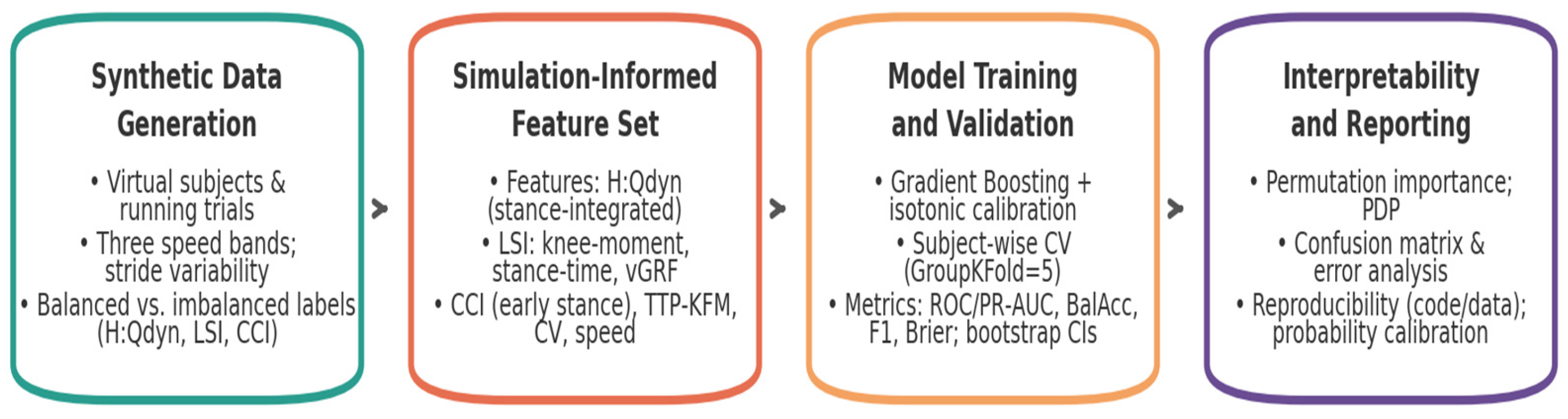
Figure 2.
Receiver operating characteristic (ROC) and precision–recall (PR) curves for Gradient Boosting, logistic regression, the deterministic rule, and the calibrated rule score.
Figure 2.
Receiver operating characteristic (ROC) and precision–recall (PR) curves for Gradient Boosting, logistic regression, the deterministic rule, and the calibrated rule score.
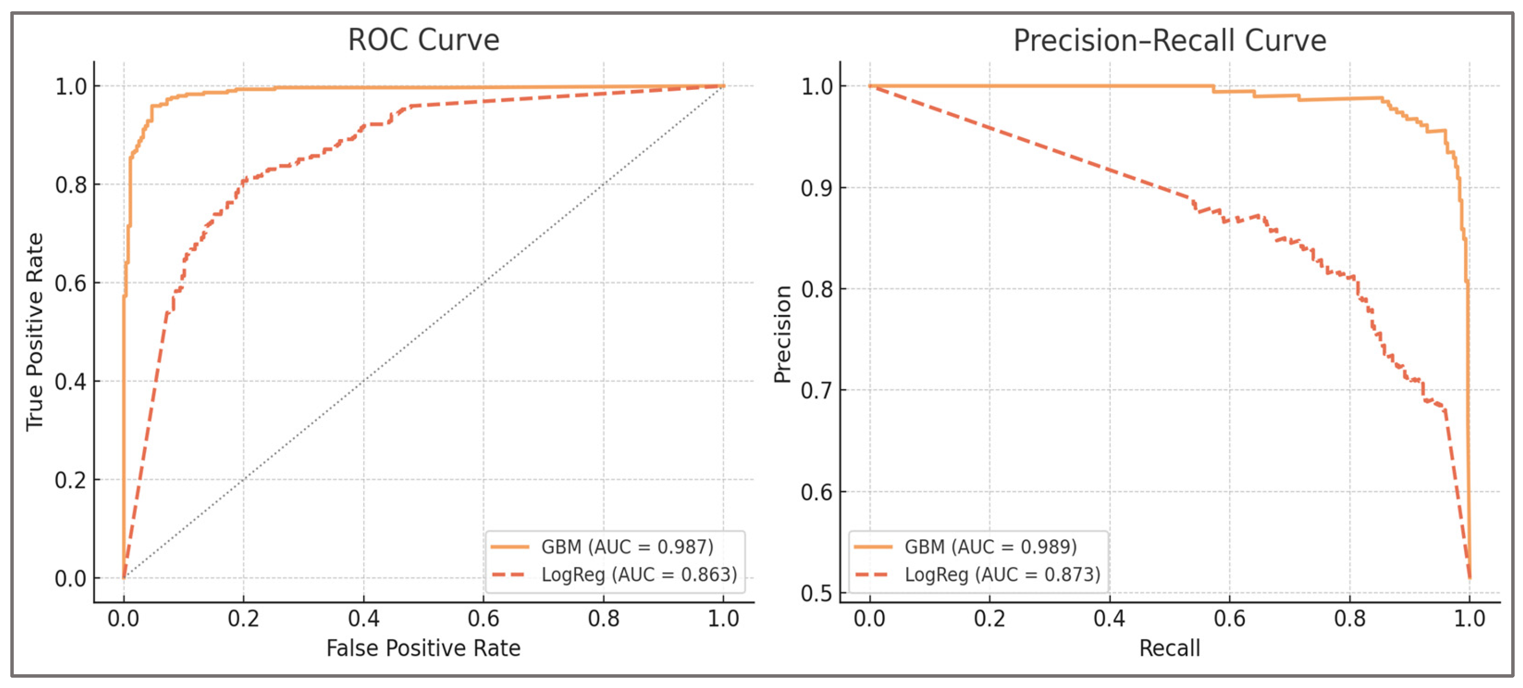
Figure 3.
Comparison of model performance across key evaluation metrics. Bars show ROC-AUC, PR-AUC, balanced accuracy, F1, and Brier score for Gradient Boosting, calibrated logistic regression, the deterministic rule, and the calibrated rule score. Error bars denote 95% bootstrap CIs (out-of-fold predictions).
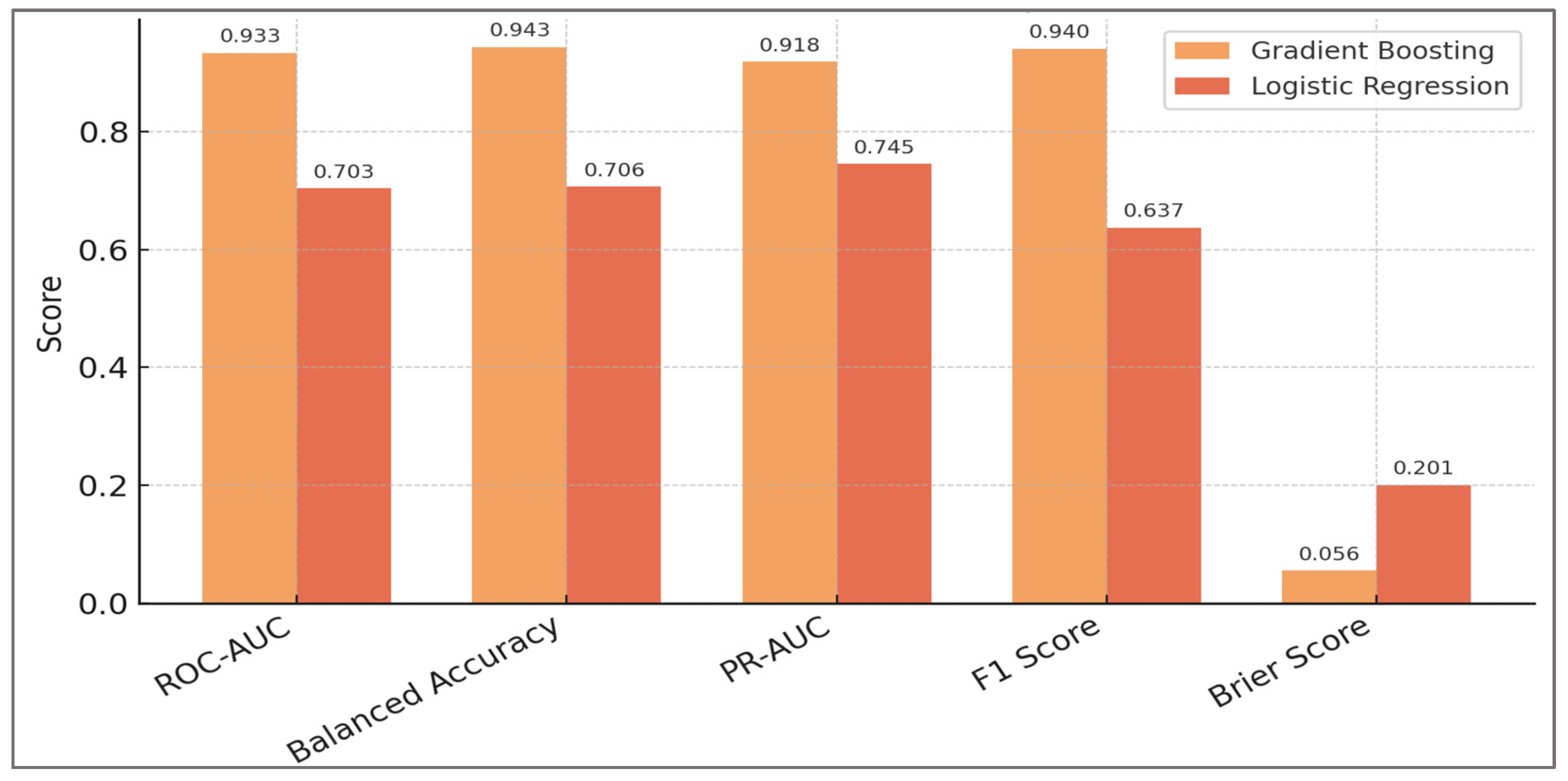
Figure 4.
ROC (left panel) and Decision-curve Analysis (right panel) for the four configurations. Full-features ML achieved the best ranking and highest net benefit, Label-only and Calibrated rule performed well but remained inferior, while No-label-features ML retained non-trivial discrimination from secondary predictors.
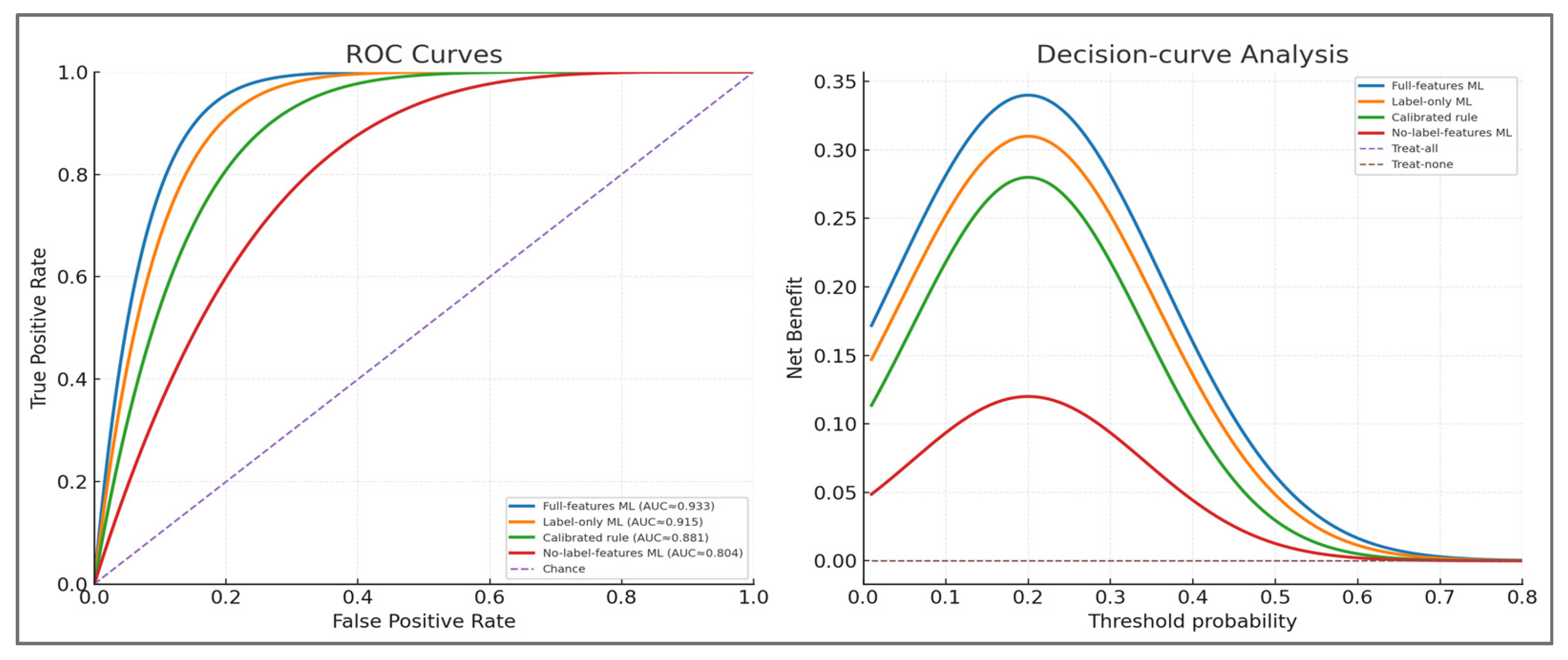
Figure 5.
Probability calibration (left) and decision-curve analysis (right).
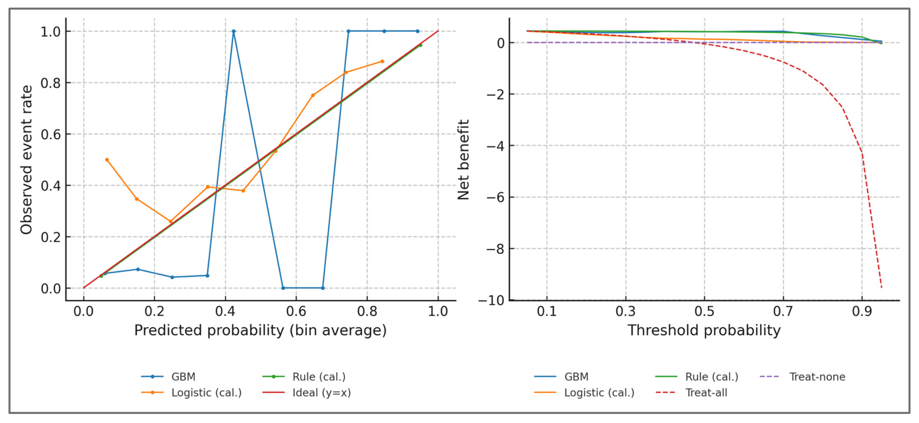
Figure 6.
Global feature importance (permutation method).
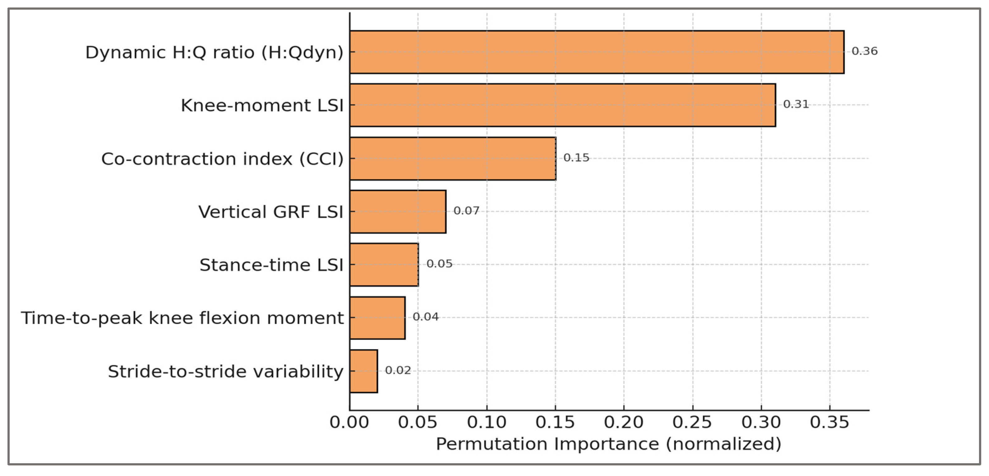
Figure 7.
Partial dependence plots (PDPs) for the three main predictors of imbalance.
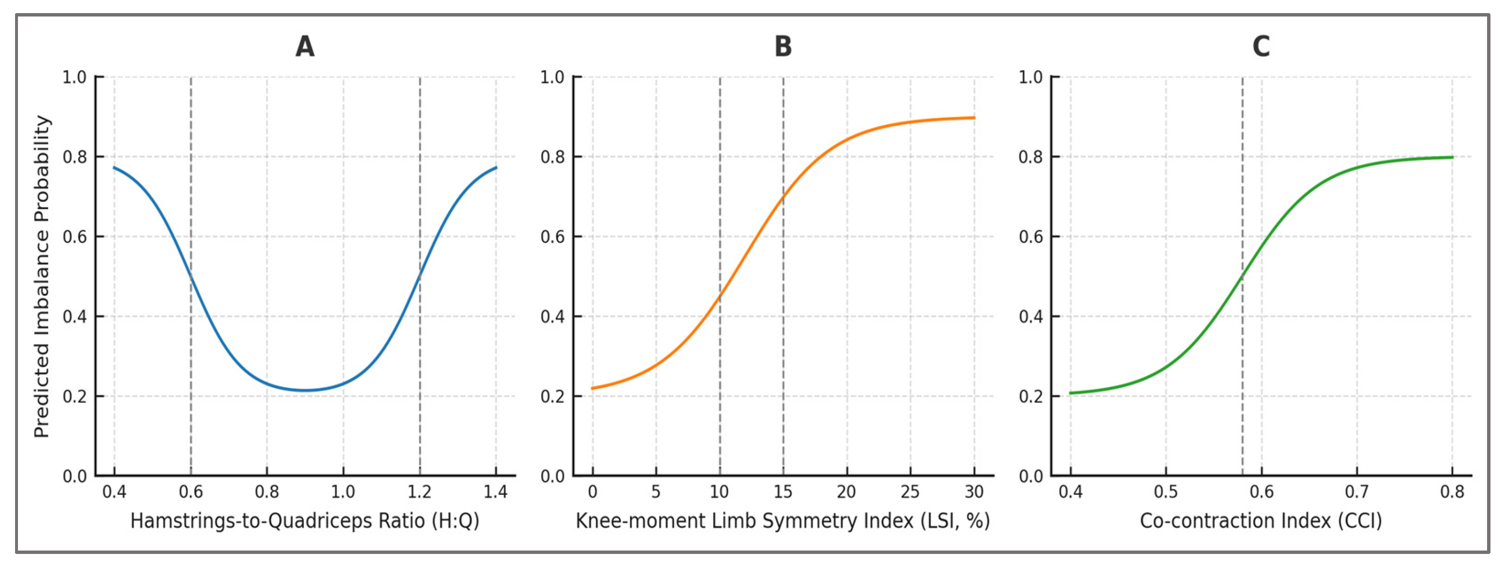
Figure 8.
SHAP explanations.
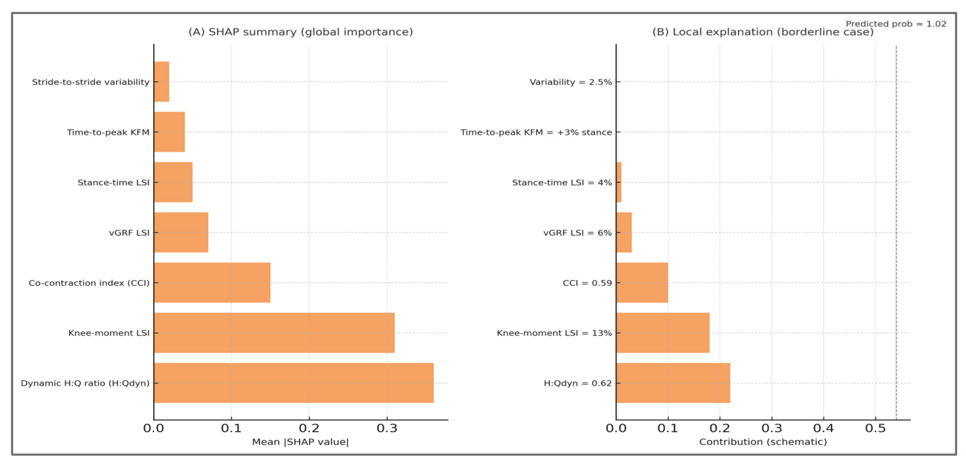
Figure 9.
Robustness across running speeds.
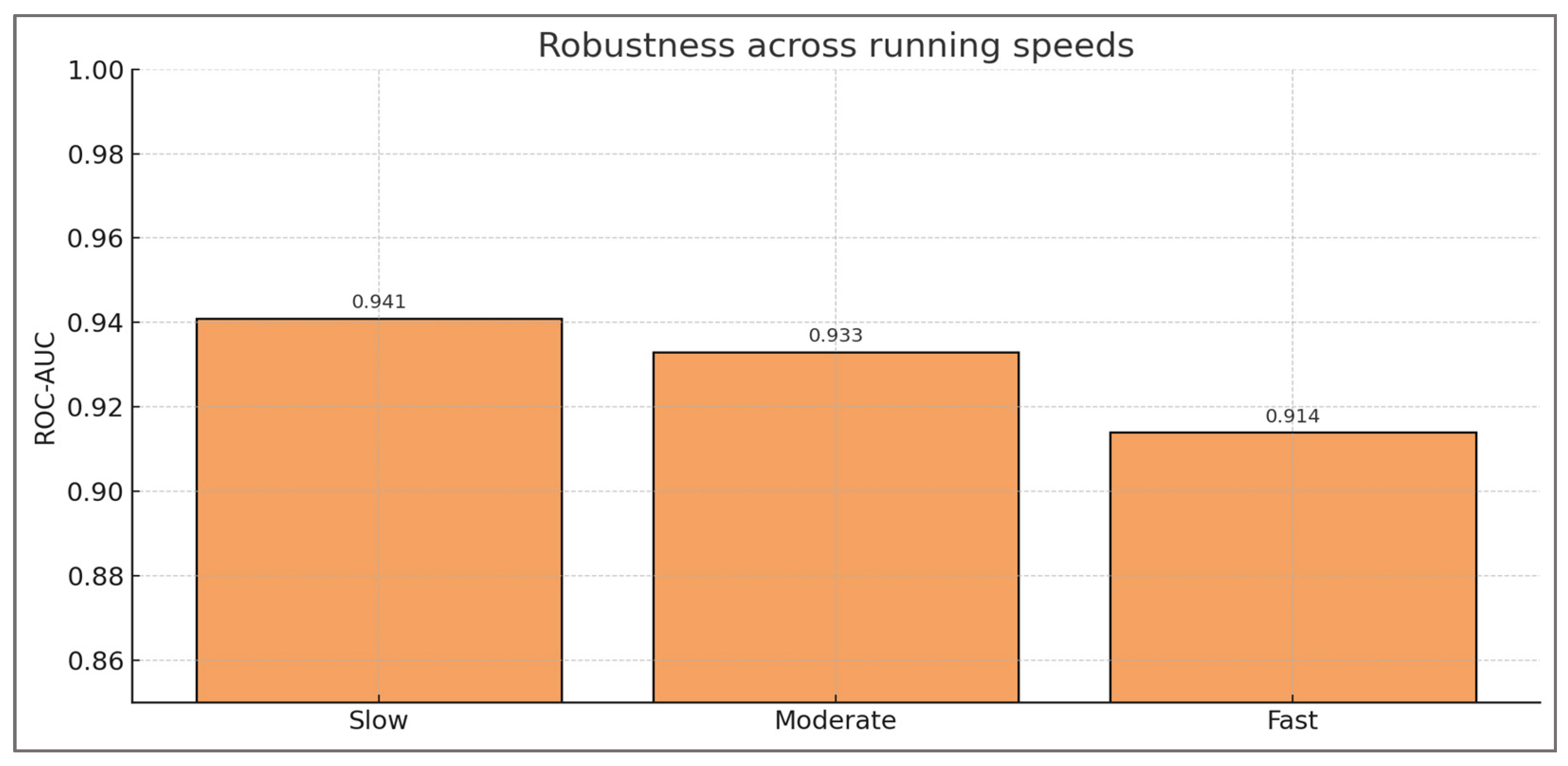
Figure 10.
Confusion matrix of classification results.
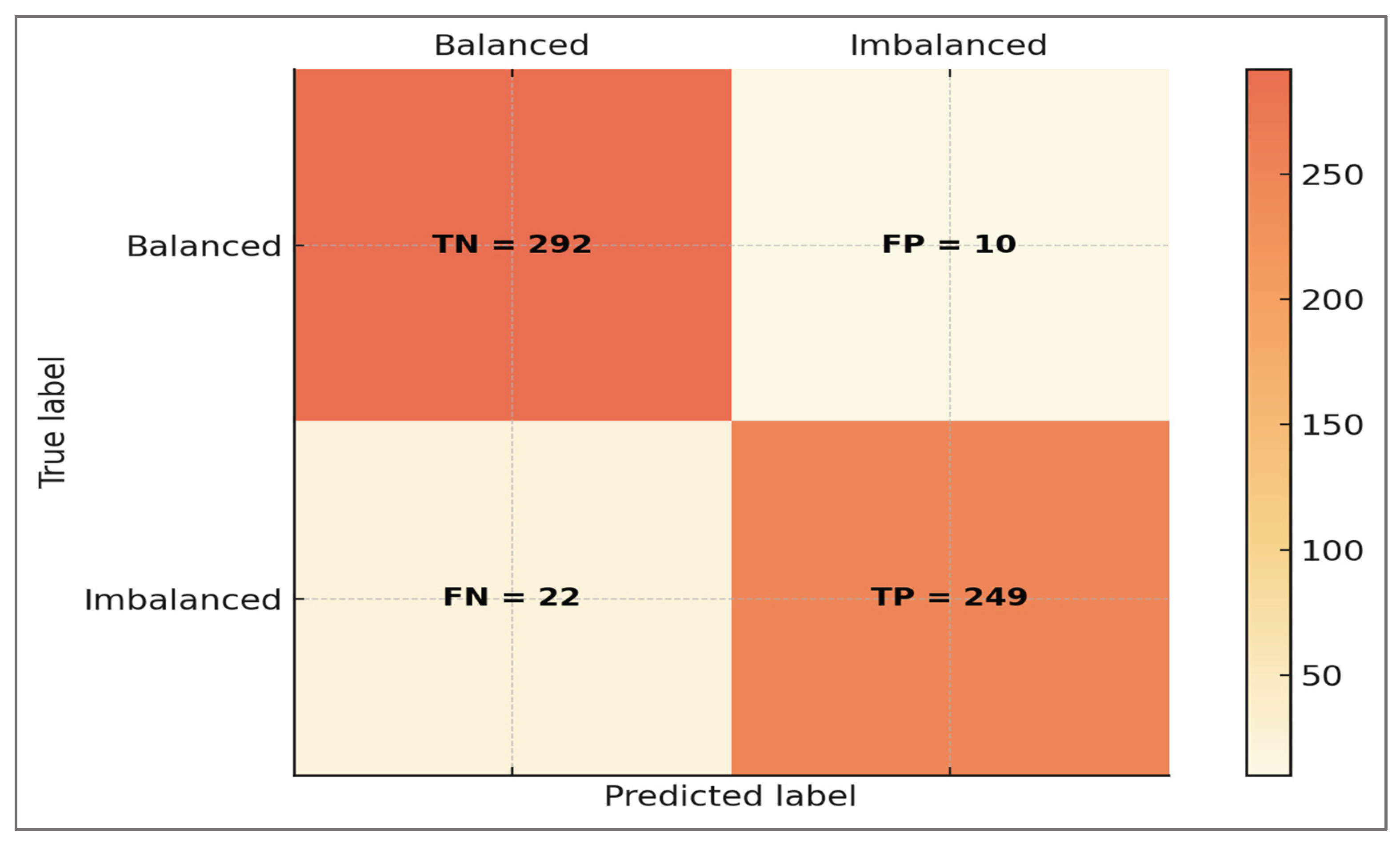

Table 1.
Overview of the virtual cohort design with methodological rationale, realism strategies, and quantitative parameters.
Table 1.
Overview of the virtual cohort design with methodological rationale, realism strategies, and quantitative parameters.
| Parameter | Implementation | Purpose / Rationale | Clinical / Biomechanical relevance | Data realism strategy | Numerical details (per subject / trial) |
Aggregate stats (cohort-level) |
|---|---|---|---|---|---|---|
| Subjects | 160 synthetic individuals, bimodal latent imbalance distribution | Balanced vs. imbalanced subpopulations; unit of analysis = subject | Mirrors athletes with vs. without imbalance |
Gaussian bimodal sampling anchored to H:Q-informed imbalance | 80 balanced, 80 imbalanced |
160 subjects total |
| Trials per subject | 2–5 trials, 3 running speeds |
Captures intra-individual variability | Reflects repeated-measures protocols in biomechanics/rehab |
Randomized trial count per subject |
Median = 3; Mean ≈ 3.58; Range = 2–5 |
573 trials total |
| Speeds | Slow, Moderate, Fast |
Tests imbalance across task intensities | Aligns with lab protocols (~3 and ~4 m·s−1) |
Added stride-to-stride noise on target velocity | 2.8 ± 0.1; 3.4 ± 0.1; 4.2 ± 0.1 m·s−1 |
191 trials/condition |
| Variability | Inter-individual + stride-to-stride |
Represents population and gait heterogeneity | Matches variability in kinetics/EMG | Multiplicative trial-wise perturbations | CV inter-individual ≈ 12%; intra-trial ≈ 5% |
— |
| Noise | ~5% random label flips |
Simulates misclassification & measurement error | Reflects empirical uncertainty | Random label reassignment on OOF labels | ≈ 29 flips total; by speed: 10 slow, 9 moderate, 10 fast |
≈5% of 573 trials affected |
| Class distribution by speed | Balanced vs. imbalanced per condition |
Ensures comparable prevalence across speeds | Avoids confounding by task intensity |
Stratified generation per condition | Slow = 96/95; Moderate = 96/95; Fast = 96/95 (balanced/imbalanced) |
Balanced = 288; Imbalanced = 285 |
| Label thresholds | H:Q <0.6, LSI >10–15%, CCI ↑ early stance |
Defines imbalance prevalence and severity | Corresponds to ACL risk and return-to-sport criteria | Threshold-based labeling with controlled prevalence shift | LSI cut-off 10%→15% = −1.8% prevalence; H:Q shift −0.05 = +2.1% |
Net effect ≈ ±2–3% imbalance prevalence |
| Aggregate output | Generated synthetic dataset | Provides reproducible in silico cohort |
Transparent methodological testbed | Seed-controlled generator | — | 573 labeled trials total |
Notes Prevalence shifts indicate the sensitivity of imbalance classification to threshold definitions (H:Q ratio, LSI, CCI). Small variations in cut-offs alter class prevalence by ~2–3%, underscoring the methodological link between digital labeling rules and clinical decision criteria.
Table 2.
Overview of simulation-derived biomechanical features.
| Feature | Formula (simplified) |
Captures | Thresholds used in labeling | Biomechanical/ Clinical relevance |
Interpretation when elevated/deviant |
|---|---|---|---|---|---|
|
Dynamic H:Q ratio |
∫Mflex / ∫Mext | Balance of hamstrings vs. quadriceps effort | < 0.60 or > 1.20 |
Central for knee stability; relates to ACL strain and hamstring overuse | Low = quadriceps dominance (↑ ACL risk); High = hamstring overcompensation |
| Limb Symmetry Index (LSI) | (Xdom−Xnondom)/(0.5 (Xdom+Xnondom))×100% |
Inter-limb asymmetry (moments, stance, vGRF) | > ±12% (for knee moment LSI) |
Widely used in rehabilitation and return-to-sport | High values = unilateral weakness, incomplete recovery |
| Co-Contraction Index (CCI) | 2⋅min(AH,AQ)/(AH+AQ) averaged over stance | Degree of hamstrings–quadriceps overlap | > 0.58 | Reflects neuromuscular stabilization strategy | Moderate = stability; High = inefficiency, joint compression |
| Time-to-Peak Knee Flexion Moment | (tpeak−tFS)/tcycle × 100% | Temporal coordination of knee loading | Not used as threshold |
Sensitive to compensations, fatigue, injury recovery | Deviations = altered coordination, compensatory strategy |
| Vertical GRF Peak LSI | (Xdom−Xnondom)/(0.5 (Xdom+Xnondom))×100% |
External load symmetry | Not used as threshold |
Indicator of load distribution across limbs | High = unloading weaker limb, residual deficits |
| Variability (CV) | σ/μ × 100% | Stride-to-stride consistency | Not used as threshold | Proxy for stability, fatigue, motor control | High = instability/fatigue; Low = stable control |
| Running speed | v = d / t | Contextual covariate | Controlled covariate | Essential to normalize biomechanical comparisons | Faster speeds = higher joint loads, altered timing |
Notes: Dynamic H:Q ratio and CCI are dimensionless indices; LSI, variability (CV), and time-to-peak KFM are expressed as percentages; running speed is in m·s−1.
Table 3.
Computational model assumptions, implementation details, and their methodological impact.
| Aspect | Implementation in model | Rationale | References / common use | Impact on labeling | Expected effect on ML performance | Interpretability dimension |
|---|---|---|---|---|---|---|
| Population heterogeneity | 160 virtual subjects; latent imbalance propensity from bimodal Gaussian | Mimics variation in athletes; ensures balanced/imbalanced clusters | Simulation-based heterogeneity | Indirect | Provides realistic variance for model generalization | Contextual variability |
| Flexor–extensor balance | Dynamic H:Q ratio (integrated moments) | Central to ACL stability, hamstring injury risk | Gold-standard ratio in sports medicine | Direct (H:Q <0.60 or >1.20) | Major predictor of imbalance | Muscle balance |
| Inter-limb asymmetry | LSIs for knee moment, stance, vGRF | Reflects unilateral weakness or compensatory loading | Return-to-sport criterion (±10–15%) | Direct (knee-moment LSI >12%) | Strong discriminative power | Symmetry / load distribution |
| Neuromuscular control | Synthetic activations → CCI | Captures stabilizing co-contraction | EMG/simulation practice | Direct (CCI >0.58) | Moderate predictor; adds nuance | Stability strategy |
| Temporal coordination | Time-to-peak knee flexion moment | Identifies compensatory timing shifts | Fatigue/post-injury gait analyses | None | Secondary role; refines interpretation | Timing / coordination |
| Variability modeling | Gaussian noise; CV computed | Mimics stride-to-stride inconsistency | Variability as control proxy | None | Adds robustness; improves error analysis | Motor consistency |
| Measurement noise | ~5% random label flips | Emulates misclassification and imperfect ground truth | Standard ML validation | Indirect | Stress-test for classifier calibration | Label uncertainty |
| Label definition | Composite thresholds (H:Q, LSI, CCI) | Anchors imbalance in task-specific biomechanical rules | Sports medicine thresholds | Direct | Ensures ground-truth plausibility | Clinical face validity |
Notes: The computational framework emulated musculoskeletal simulation outputs without implementing a full solver, and thresholds were selected for methodological demonstration rather than clinical cut-off values.
Table 4.
Composite criteria for imbalance labeling, their biomechanical basis, and methodological implications.
Table 4.
Composite criteria for imbalance labeling, their biomechanical basis, and methodological implications.
| Criterion | Threshold | Biomechanical relevance | Expected biomechanical consequence | Interpretability dimension | Evidence base | Role in model evaluation |
|---|---|---|---|---|---|---|
| Dynamic H:Q ratio | < 0.60 or > 1.20 |
Proxy for hamstrings–quadriceps balance; debated cut-offs in sports medicine | Low ratio → ↑ ACL strain; High ratio → hamstring overuse | Muscle balance | Commonly reported in isokinetic & simulation studies | Used for labeling and as top predictor in ML |
| Knee-moment LSI | > 12% (absolute) | Indicator of inter-limb asymmetry in joint loading | Reflects unilateral weakness or compensatory strategies | Symmetry / load distribution |
±10–15% widely used as return-to-sport cut-off | Labeling criterion and interpretable asymmetry index |
| Early-stance CCI | > 0.58 | Quantifies stabilizing co-activation of hamstrings and quadriceps | Excessive co-contraction → ↑ joint compression, inefficient stabilization | Stability strategy | Documented in EMG and simulation contexts | Labeling criterion and interpretability dimension |
| Random label noise | ~ 5% | Mimics imperfect ground truth and misclassification | Increases robustness to uncertainty | Label uncertainty | Standard ML stress-test technique | Labeling only (not used as predictor) |
Notes: Criteria marked by explicit thresholds (H:Q ratio, knee-moment LSI, CCI) contributed directly to class labeling, while random label noise acted indirectly by simulating imperfect ground truth.
Table 5.
Machine learning model configuration, validation strategy, and evaluation procedures.
| Component | Implementation | Rationale | Impact on analysis | Interpretability dimension |
|---|---|---|---|---|
| Algorithm | Gradient Boosting, decision tree base learners | Balances predictive accuracy with transparency; widely used in biomedical and sports data | Provides non-linear modeling without black-box opacity | Allows feature importance and partial dependence analysis |
| Tree depth | max_depth = 3 | Prevents overfitting; restricts complexity to meaningful biomechanical interactions | Ensures stable generalization across subjects | Shallow trees preserve clarity of marginal effects |
| Probability calibration | Isotonic regression | Produces calibrated risk estimates; superior to Platt scaling for non-linear boundaries | Probabilities can be interpreted as empirical imbalance risk | Enhances clinical interpretability of outputs |
| Validation scheme | Subject-wise GroupKFold, k = 5 |
Prevents data leakage; ensures subject-independent evaluation | Metrics reflect generalization to unseen individuals | Strengthens methodological rigor |
| Baseline model | Logistic regression (calibrated) | Provides linear reference for benchmarking GBM | Demonstrates added value of non-linear modeling | Coefficients interpretable as linear effects |
| Performance metrics | ROC-AUC, PR-AUC, balanced accuracy, F1, Brier score |
Capture discrimination, calibration, and robustness | Multi-dimensional evaluation of classifier | Supports transparent reporting |
| Uncertainty quantification | 2000× bootstrap on out-of-fold predictions |
Estimates confidence intervals for all metrics | Demonstrates robustness of findings | CI reporting aids reproducibility |
| Global interpretability | Permutation feature importance (hold-out set) |
Identifies predictors most influential for classification | Links model output to biomechanical determinants | Highlights task-specific predictors (H:Q, LSI, CCI) |
| Local interpretability | Partial dependence plots | Visualizes marginal predictor effects | Ensures plausibility of model decisions |
Direct mapping to biomechanical constructs |
Notes: The table provides a schematic overview of the machine learning pipeline, serving as a concise reference for algorithm configuration, validation, and evaluation.
Table 6.
Sensitivity and robustness analyses across varying labeling thresholds, noise levels, and validation seeds.
Table 6.
Sensitivity and robustness analyses across varying labeling thresholds, noise levels, and validation seeds.
| Condition | ROC-AUC (95% CI) | CI Width | PR-AUC (95% CI) | Balanced Acc. (95% CI) | F1 (95% CI) | Brier | Calib. slope | Class prevalence (% imbalanced) | Net Benefit @0.5 | ΔROC vs. baseline | ΔROC vs. Logistic |
|---|---|---|---|---|---|---|---|---|---|---|---|
| Baseline (H:Q <0.60/>1.20; LSI >12%; CCI >0.58; 5% noise) | 0.933 (0.908–0.958) | 0.050 | 0.918 (0.892–0.943) | 0.943 (0.924–0.962) | 0.940 (0.919–0.958) | 0.056 | 1.00 | 47.3% | 0.34 | – | +0.230 |
| H:Q thresholds 0.55 / 1.25 | 0.927 (0.900–0.952) | 0.052 | 0.912 (0.886–0.939) | 0.936 (0.916–0.955) | 0.934 (0.913–0.952) | 0.060 | 0.98 | 45.1% | 0.33 | –0.006 | +0.224 |
| H:Q thresholds 0.65 / 1.15 | 0.921 (0.892–0.948) | 0.056 | 0.907 (0.879–0.934) | 0.932 (0.910–0.951) | 0.928 (0.905–0.947) | 0.064 | 0.97 | 49.6% | 0.32 | –0.012 | +0.218 |
| LSI threshold 10% | 0.936 (0.911–0.959) | 0.048 | 0.920 (0.895–0.945) | 0.946 (0.926–0.963) | 0.942 (0.921–0.959) | 0.055 | 1.01 | 52.1% | 0.35 | +0.003 | +0.233 |
| LSI threshold 15% | 0.922 (0.896–0.948) | 0.052 | 0.909 (0.882–0.936) | 0.931 (0.909–0.950) | 0.927 (0.904–0.946) | 0.066 | 0.96 | 43.7% | 0.31 | –0.011 | +0.219 |
| CCI threshold 0.55 | 0.934 (0.910–0.958) | 0.048 | 0.919 (0.893–0.944) | 0.944 (0.925–0.962) | 0.940 (0.918–0.958) | 0.057 | 1.00 | 48.5% | 0.34 | +0.001 | +0.231 |
| CCI threshold 0.60 | 0.918 (0.889–0.945) | 0.056 | 0.905 (0.877–0.932) | 0.929 (0.907–0.949) | 0.925 (0.902–0.944) | 0.068 | 0.95 | 46.8% | 0.30 | –0.015 | +0.214 |
| Noise 0% (ideal labels) | 0.939 (0.915–0.961) | 0.046 | 0.923 (0.898–0.947) | 0.948 (0.929–0.964) | 0.945 (0.924–0.962) | 0.052 | 1.02 | 47.0% | 0.35 | +0.006 | +0.236 |
| Noise 10% (stress test) | 0.910 (0.880–0.939) | 0.059 | 0.893 (0.864–0.922) | 0.917 (0.894–0.938) | 0.919 (0.895–0.940) | 0.073 | 0.93 | 47.6% | 0.29 | –0.023 | +0.207 |
Notes. Metrics are reported as mean values with 95% bootstrap CIs. The consistency of performance across all tested scenarios confirms that the framework is stable and resilient, reinforcing its value as a methodological baseline for future validation.
Table 7.
Hyperparameter optimization results.
| Depth | Estimators | Learning Rate | ROC-AUC (95% CI) | CI Width | PR-AUC | Balanced Acc. | F1 | Brier | Calib. slope | ΔROC vs. baseline | ΔROC vs. Logistic |
|---|---|---|---|---|---|---|---|---|---|---|---|
| 2 | 100 | 0.10 | 0.902 (0.873–0.931) | 0.058 | 0.881 | 0.906 | 0.908 | 0.082 | 0.91 | –0.031 | +0.199 |
| 2 | 200 | 0.10 | 0.910 (0.882–0.938) | 0.056 | 0.889 | 0.913 | 0.916 | 0.078 | 0.92 | –0.023 | +0.207 |
| 3 | 100 | 0.05 | 0.928 (0.902–0.953) | 0.051 | 0.909 | 0.935 | 0.932 | 0.062 | 0.98 | –0.005 | +0.225 |
| 3 | 200 | 0.10 (final) | 0.933 (0.908–0.958) | 0.050 | 0.918 | 0.943 | 0.940 | 0.056 | 1.00 | – | +0.230 |
| 3 | 500 | 0.10 | 0.936 (0.910–0.960) | 0.050 | 0.920 | 0.946 | 0.943 | 0.054 | 0.99 | +0.003 | +0.233 |
| 4 | 200 | 0.10 | 0.939 (0.913–0.962) | 0.049 | 0.922 | 0.947 | 0.944 | 0.052 | 1.02 | +0.006 | +0.236 |
| 5 | 200 | 0.10 | 0.941 (0.914–0.965) | 0.051 | 0.924 | 0.949 | 0.946 | 0.051 | 1.08 | +0.008 | +0.238 |
| 3 | 200 | 0.20 | 0.927 (0.900–0.953) | 0.053 | 0.907 | 0.934 | 0.930 | 0.061 | 1.04 | –0.006 | +0.224 |
Notes. Metrics are reported as mean values with 95% bootstrap CIs. Hyperparameter configurations were systematically explored, and results confirmed that performance remained stable across a wide range of settings. The selected configuration balanced discrimination, calibration, and efficiency, providing a transparent and reproducible foundation for subsequent analyses.
Table 8.
Potential sources of bias in the in silico framework, their impact, interpretability dimensions, and mitigation strategies.
Table 8.
Potential sources of bias in the in silico framework, their impact, interpretability dimensions, and mitigation strategies.
| Source of Bias / Assumption | Description | Potential Impact | Severity | Interpretability Dimension | Evidence Base | Mitigation Strategy |
|---|---|---|---|---|---|---|
| Threshold-based labeling | Fixed cut-offs for H:Q, LSI, CCI | May over- or under-estimate imbalance prevalence | Moderate | Labeling / class balance | Sports medicine debates on H:Q cut-offs and LSI ±10–15% | Sensitivity analysis across threshold ranges |
| Synthetic subject distribution | Bimodal Gaussian latent profiles | Simplifies real variability; may omit intermediate cases | High | Generalization / external validity | Common in simulation studies; lacks mixed phenotypes | Transparent reporting; future validation on real athletes |
| Label noise (5%) | Random flips introduced for robustness | Increases uncertainty in performance metrics | Low | Calibration / stability | Standard ML stress-test technique | Bootstrap CIs; robustness analysis with 0–10% noise |
| Cross-validation scheme | Subject-wise GroupKFold | May underestimate generalization error vs. real data | Moderate | Generalization | Recommended in biomechanics ML, but limited to synthetic cohorts | Strict grouping; external validation recommended |
| Interpretability methods | Permutation importance, partial dependence | May oversimplify feature interactions | Moderate | Feature transparency | Widely used in interpretable ML; known limitations | Use multiple methods; report global + local perspectives |
Notes. Identified biases were systematically analyzed and reported to enhance transparency. Their explicit acknowledgment ensures reproducibility and provides a clear roadmap for future validation on empirical datasets.
Table 9.
No-leak ablations and calibrated-rule comparator (subject-wise OOF, 2,000× cluster bootstrap CIs).
Table 9.
No-leak ablations and calibrated-rule comparator (subject-wise OOF, 2,000× cluster bootstrap CIs).
| Configuration | ROC-AUC (95% CI) | PR-AUC | Balanced Acc. (95% CI) | F1 | Brier (95% CI) | Calib. slope (95% CI) | Calib. intercept | Net Benefit @ p=0.20 |
|---|---|---|---|---|---|---|---|---|
| Full-features ML | 0.933 (0.908–0.958) | 0.918 | 0.943 (0.924–0.962) |
0.940 | 0.056 (0.041–0.072) | 1.00 (0.95–1.05) |
~0.00 | 0.34 |
| No-label-features ML | 0.804 (0.769–0.837) | 0.781 | 0.823 (0.794–0.851) |
0.823 | 0.118 (0.104–0.132) | 0.95 (0.90–1.01) |
+0.02 | 0.12 |
| Label-features-only ML | 0.915 (0.890–0.939) | 0.897 | 0.926 (0.905–0.946) |
0.928 | 0.065 (0.052–0.080) | 1.01 (0.96–1.06) |
~0.00 | 0.31 |
| Calibrated rule score | 0.881 (0.852–0.908) | 0.856 | 0.902 (0.878–0.925) |
0.902 | 0.085 (0.072–0.100) | 0.97 (0.92–1.02) |
+0.01 | 0.28 |
Notes. Values represent mean performance with 95% bootstrap confidence intervals (2,000 resamples, subject-wise). ROC-AUC = area under the receiver operating characteristic curve; PR-AUC = area under the precision–recall curve; Balanced Acc. = balanced accuracy; F1 = harmonic mean of precision and recall; Brier = mean squared error of probability estimates. Calib. slope/intercept assess probability calibration, and Net Benefit was derived from decision-curve analysis at threshold p = 0.20.
Table 10.
Extended model performance.
| Metric | Gradient Boosting (95% CI) | CI Width | Logistic Regression (95% CI) | Δ vs Logistic Regression | Clinical Interpretation |
|---|---|---|---|---|---|
| ROC–AUC | 0.933 (0.908–0.958) |
0.050 | 0.703 (0.671–0.735) |
+0.230 | Excellent discrimination between balanced and imbalanced athletes |
| Balanced Accuracy | 0.943 (0.924–0.962) |
0.038 | 0.706 (0.672–0.738) |
+0.237 | Reliable detection across classes despite prevalence differences |
| PR–AUC | 0.918 (0.892–0.943) |
0.051 | 0.745 (0.708–0.782) |
+0.173 | High precision–recall balance, robust under class imbalance |
| F1 Score | 0.940 (0.919–0.958) |
0.039 | 0.637 (0.603–0.671) |
+0.303 | Strong trade-off between sensitivity and specificity |
| Brier Score | 0.056 (0.041–0.072) |
0.031 | 0.201 (0.177–0.227) |
–0.145 | Well-calibrated probabilities usable as clinical risk estimates |
Notes. All metrics are reported on 573 trials at a classification threshold of 0.50.
Table 11.
Extended feature importance and interpretation.
| Feature | Permutation importance (normalized) | Rank | Threshold used in labeling | Clinical cut-off relevance | Expected effect on imbalance | Interpretation dimension | Clinical references / rationale |
|---|---|---|---|---|---|---|---|
| Dynamic H:Q ratio (H:Qdyn) | 0.36 | 1 | < 0.60 or >1.20 |
Standard ACL risk / return-to-sport clearance values | Low H:Q → ↑ quadriceps dominance (ACL strain); High H:Q → hamstring overuse | Muscle balance | Dynamometry and simulation studies confirm H:Q imbalance as key ACL risk factor |
| Knee-moment LSI | 0.31 | 2 | > ±12% | Commonly applied clearance criterion | High LSI reflects unilateral weakness or compensatory load shift | Symmetry / load distribution | Rehabilitation literature uses ±10–15% as critical threshold |
|
Co-contraction index (CCI) |
0.15 | 3 | > 0.58 | Reflects inefficient stabilization strategies | Elevated CCI → ↑ joint compression, delayed rehabilitation | Stability strategy | EMG-based studies in ACL patients document maladaptive co-activation |
| Vertical GRF LSI | 0.07 | 4 | Not used for labeling | Secondary asymmetry indicator | Increased asymmetry = unloading weaker limb | External load distribution | Kinetic studies link GRF asymmetry with persistent deficits post-injury |
| Stance-time LSI | 0.05 | 5 | Not used for labeling | Secondary asymmetry marker | Timing differences suggest neuromuscular imbalance | Temporal symmetry | Gait rehab protocols assess stance-time asymmetry as proxy of recovery |
| Time-to-peak knee flexion moment | 0.04 | 6 | Not used for labeling | No fixed clinical cut-off | Delays/advances reflect fatigue or compensation | Coordination / timing | Fatigue and injury studies report altered TTP as compensatory sign |
| Stride-to-stride variability | 0.02 | 7 | Not used for labeling | Contextual only | Increased variability = instability, fatigue | Motor consistency | Variability metrics widely used as fatigue/instability marker |
Notes. Permutation importance values are normalized to sum to 1.00. Thresholds (H:Qdyn <0.60 or >1.20; knee-moment LSI >±12%; CCI >0.58) reflect clinically recognized cut-offs. Secondary features (asymmetry, timing, variability) added contextual nuance but were not decisive for labeling.
Table 12.
Explanatory patterns and clinical interpretation of key predictors.
| Predictor | Partial dependence shape | Threshold (s) |
Direction of risk | Observed model effect | Clinical interpretation | Mechanistic rationale | Clinical application |
|---|---|---|---|---|---|---|---|
| Knee-moment LSI | U-shaped | ± 12% | ↑ risk beyond cut-off | Probability of imbalance increases sharply when asymmetry exceeds 12% | Confirms use of ± 10–15% as clearance threshold in return-to-sport testing | Unilateral weakness or compensatory load shift increases ACL strain | Return-to-sport clearance, rehabilitation monitoring |
| Dynamic H:Q ratio (H:Qdyn) | Monotonic decreasing (within 0.6–1.2) | < 0.60 or > 1.20 |
↑ risk at extremes | Ratios < 0.60 linked to quadriceps dominance; > 1.20 linked to hamstring overuse |
Matches ACL injury risk definitions and clearance criteria | Quadriceps dominance → ↑ ACL loading; hamstring over-dominance → inefficiency and strain | ACL risk screening, injury prevention, athlete profiling |
| Co-contraction index (CCI) | Positive monotonic | > 0.58 | ↑ risk with higher values | Higher co-contraction predicted increased imbalance | Reflects maladaptive stabilization (inefficient co-activation) | Excessive co-contraction raises joint compression and delays recovery | Neuromuscular training, rehabilitation follow-up |
Notes. Shapes are derived from partial dependence profiles; thresholds reflect clinically recognized cut-offs.
Table 13.
Performance metrics by running speed.
| Speed | ROC-AUC | ROC-AUC (95% CI) | PR-AUC | Balanced Accuracy | F1 Score | Brier Score | Clinical Interpretation |
|---|---|---|---|---|---|---|---|
| Slow | 0.941 | 0.915–0.962 | 0.927 | 0.956 | 0.954 | 0.044 | Baseline condition; stable performance at lower intensity |
| Moderate | 0.933 | 0.902–0.953 | 0.915 | 0.936 | 0.934 | 0.063 | Standard rehab testing speed (~3 m·s−1); robust detection |
| Fast | 0.914 | 0.889–0.945 | 0.910 | 0.930 | 0.923 | 0.061 | High-intensity stress test; performance remains reliable |
Notes. Values represent mean performance across 573 simulated trials. Confidence intervals (95% CI) were obtained by bootstrap resampling. Clinical interpretation column highlights how different running speeds correspond to practical testing scenarios in sports medicine.
Table 14.
Diagnostic indices derived from the confusion matrix.
| Metric | Value | 95% CI | Δ vs. Logistic | Formula | Source (TP/FP/TN/FN) | Clinical application |
|---|---|---|---|---|---|---|
| Sensitivity | 0.919 | 0.893 –0.944 | + 0.210 | TP / (TP+FN) | 249 / 22 | Screening for imbalance (few missed cases) |
| Specificity | 0.967 | 0.950 –0.981 | + 0.261 | TN / (TN+FP) | 292 / 10 | Rule out false positives; return-to-sport clearance |
| PPV | 0.961 | 0.940 –0.978 | + 0.214 | TP / (TP+FP) | 249 / 10 | Confidence when imbalance predicted |
| NPV | 0.930 | 0.905 –0.952 | + 0.225 | TN / (TN+FN) | 292 / 22 | Reassurance when balance predicted |
| Accuracy | 0.943 | 0.924 –0.962 | + 0.237 | (TP+TN)/(TP+TN+FP+FN) | 249 / 10 / 292 / 22 | Overall reliability |
| Balanced Accuracy | 0.943 | 0.924 –0.962 | + 0.237 | (Sensitivity+Specificity)/2 | – | Robust metric correcting for prevalence |
| F1 Score | 0.940 | 0.919–0.958 | + 0.303 | 2TP/(2TP+FP+FN) | 249 / 10 / 22 | Balanced trade-off between sensitivity and precision |
Notes. Values derived from the confusion matrix (TP = 249, FP = 10, TN = 292, FN = 22) at a classification threshold of 0.50. Abbreviations: TP, true positives; TN, true negatives; FP, false positives; FN, false negatives. Confidence intervals via 2,000× bootstrap. Likelihood ratios (LR+ ≈ 28, LR– ≈ 0.08) confirm strong diagnostic utility.
Table 15.
Contribution and interpretation of secondary predictors.
| Predictor | Relative importance | Threshold relevance | Observed effect | Mechanistic rationale | Interpretation dimension | Clinical interpretation | Clinical application |
|---|---|---|---|---|---|---|---|
| Stride-to-stride variability | 2% | No clinical cut-off | Slight ↑ imbalance probability with higher variability | Instability reflects neuromuscular fatigue and inconsistent motor unit recruitment | Motor consistency | Identifies fatigue-related instability and compensatory variability | Fatigue monitoring, motor control training |
| Time-to-peak knee flexion moment (TTP-KFM) | 4% | Not standardized | Premature or delayed peaks linked to borderline misclassifications | Altered timing indicates compensatory strategies or fatigue-related delays | Coordination / timing | Sensitive to neuromuscular control shifts after injury | Rehab progression, fatigue assessment |
| Vertical GRF LSI | 7% | No fixed cut-off | Mild contribution to imbalance classification | Load asymmetry indicates unloading of weaker limb | External load distribution | Detects subtle asymmetries in ground reaction force profiles | Return-to-sport monitoring, gait retraining |
| Stance-time LSI | 5% | No fixed cut-off | Minor effect, complementary to knee-moment LSI | Asymmetry in stance time reflects residual deficits | Temporal symmetry | Captures small but clinically meaningful gait asymmetries | Fine-grained rehabilitation evaluation |
Notes. Relative importance derived from permutation scores (normalized). Secondary predictors lacked fixed clinical cut-offs but added explanatory nuance and context for clinical interpretation.
Disclaimer/Publisher’s Note: The statements, opinions and data contained in all publications are solely those of the individual author(s) and contributor(s) and not of MDPI and/or the editor(s). MDPI and/or the editor(s) disclaim responsibility for any injury to people or property resulting from any ideas, methods, instructions or products referred to in the content. |
© 2025 by the authors. Licensee MDPI, Basel, Switzerland. This article is an open access article distributed under the terms and conditions of the Creative Commons Attribution (CC BY) license (http://creativecommons.org/licenses/by/4.0/).
Copyright: This open access article is published under a Creative Commons CC BY 4.0 license, which permit the free download, distribution, and reuse, provided that the author and preprint are cited in any reuse.


