
Submitted:
18 November 2025
Posted:
18 November 2025
You are already at the latest version
Abstract
Throughout the history of scientific discovery, the question of could a machine be able to find the laws of nature directly from observed data without relying on any prior information has been unimaginable until the emergence of modern-day computing and Artificial Intelligence. We develop a framework as an operator operation, evaluation, and optimization for a decision-machine to conduct scientific discovery: both nature’s “behavior” and the decision-machine’s “actions” are modeled with a formalized system under Hilbert Space; three inductive rules are utilized to evaluate the decision-machine’s performance; and the evolutionary algorithm is applied to optimize the best way to reconstruct the historical data and effectively predict its future. A simulated random dataset is used to show that the decision-machine is able to reasonably reconstruct the experimental data and effectively predict the future. Crucially, our developed framework is a versatile and experimentally feasible tool for conducting scientific discovery by machine that has broad implications for forecasting, AI for science, and fundamental scientific discovery of the natural and social sciences.
Keywords:
scientific discovery
; decision‐machine
; quantum superposition
; natural selection
; quantum‐like evolutionary algorithm
; genetic programming
; inductive rules
1. Introduction
The essence of scientific discovery is to seek out the laws that govern nature as effectively as possible; in which there are four main parts that comprise of all generic scientific discovery – nature, observer, measuring instrument, and the observed data. Nature is what is being studied, its infinite possibilities are the main objective of scientific discovery. The observers are who that’s conducting the studying, their proposed hypothesizes are the subjective of scientific discovery. The measuring instrument is the tool of scientific discovery, and is the apparatus that directly interacts with nature to record data. Observed data is the medium of scientific discovery, the data that’s recorded by the apparatus is the main target for the observer when studying nature [1-3].
Under the current established scientific method, the goal of the observer is to find the laws of nature by proposing a hypothesis, formulating experiments, and validating the original hypothesis [4-6]. For these hypothesis’ to be considered sufficient enough to become a theory, they have to meet two simple criteria: 1) reconstruct the experimental data, and 2) make effective forecasts of future data.
There are three main parts for the observer when conducting scientific discovery: observed data X, proposed hypotheses H, and validation criteria V.
- 1)
- : The observer’s medium of scientific discovery.
- 2)
- : The proposed hypotheses of the observer.
- 3)
- : The metric used to validate the proposed hypothesis.
With the rise of computing power and artificial intelligence, the question of whether a machine could discover the laws of nature has become how – in which we ask:
Could we develop a machine to find the laws of nature directly from observed data by means of data-driven machine learning without relying on any prior knowledge?
In this Letter, we propose a framework to develop a decision-machine to conduct scientific discovery in three distinct parts.
First, a formalized symbol framework to describe both nature’s “behavior” and the decision-machine’s “actions” is defined; second, follow three predetermined inductive rules to evaluate the decision-machine’s performance; and third, continually optimize the scientific discovery process with an evolutionary algorithm.
A simulated random-walk dataset is generated for the decision-machine to “study”. We show that the decision-machine is able to reconstruct its historical data with a MAE of 4.26 and produce 3 forecasts with MAE of 8.74, 6.9, and 6.43; and MAPE of 9.66, 7.06, and 6.82. Remarkably the decision-machine is able to produce a better MAE than traditional methods in reconstructing the historical data, and is able to produce a better MAE and MAPE on average when forecasting future data.
2. Setup
We consider a generated one dimensional randomly fluctuating dataset; which is generated by a predefined program following two simple rules:
- 1)
- Randomly generate 1 or -1; if 1 then the succeeding point will be greater than the preceding one; if -1 then the succeeding point will be lesser than the preceding one.
- 2)
- Randomly generate a number from ; this number will be the distance between the two subsequent (consecutive) data points.
The program generates 35 data points with the starting point of 100 as in (1).
This generated dataset is then used as the raw data the decision-machine will study, reconstruct, and subsequently produce effective forecasts of. The generated dataset is split into two respective portions – training and verify. Of the 35 points, 1-29 is used as training and 30-35 is used as verify data.
3. Model
For the data generated, and for any one-dimensional sequential data in general, there are two main characteristics – 1) the succeeding point either moves up or down relative to the preceding point; and 2) there is a certain distance (change of movement) between the successive points. The main problem for the decision-machine conducting scientific discovery is how to successfully find both the trend movement and the distance movement of nature; in which nature does not tend to laminate all the information regarding these two characteristics.
For human observers, traditional scientific discovery has strictly followed an entity – properties – structure approach, one which has led to the formulation of concepts of force, energy, and wave-function, etc.; this approach has widely used differential equations to formulate a function for describing natural phenomena. However, nature’s “behavior” tends to be “chaotic”, and the uncertainty of the real world makes it difficult to directly find a function that can explain all observed phenomena.
From an information perspective, the decision-machine will conduct scientific discovery abiding by an event – information – operation approach; events present the decision-machine with information not property. With event being what is studied, information being the message “passed along” between nature and the decision-machine, and operation being the series of “actions” performed by the decision-machine to learn more about nature.
Instead of directly attempting to formulate a function, we can transform the observed dataset into an event series, with each subsequent data point and the distance between successive points representing an event “performed” by nature as in (2).
For the decision-machine to study the dataset and simulate nature, there are also two main characteristics – 1) “guess” whether the data will trend upwards or downwards, and 2) calculate the specific distance between the successive points as best as possible; the decision-machine’s “actions” to simulate nature’s movement are represented as an action sequence in (3).
To model both nature’s event and the decision-machine’s “action” under one formalized framework, the first three axioms of quantum mechanics are utilized [7-10].
The two orthogonal possible states of an event (up or down) and an action taken by the decision-machine (“guess” up or down) can be represented by a superposed state in Hilbert Space.
Nature’s event becomes (4).
The decision-machine’s action becomes (5).
For the decision-machine to reconstruct the observed dataset, corresponding density operators must be defined.
The observable (density operator) of nature’s event is in (6).
The observable (density operator) of the decision-machine’s actions is in (7).
and signifies the undetermined superposition state. Once it’s “measured”, an event actually takes place and the decision-machine takes an “action”, a projection happens as (8) and (9).
The data series is reconstructed as in (10) with that simulates nature’s “behavior”.
is utilized by the decision-machine to calculate nature’s position as in (11).
The decision-machine applies to perform an “action” that simulates nature's behavior by “deciding” whether the event will move upwards or downwards. The main goal of is to “guess” as correct as possible compared to nature’s with the greatest confidence. For each event of nature , the decision-machine’s corresponding should aim to be correct with the greatest confidence (). If this is achieved, then the decision-machine is able to simulate nature’s events series perfectly every single time.
If the position series calculated by the decision-machine perfectly overlaps with nature’s position series , then the decision-machine “discovers” the “kinetic laws” of nature.
4. Evaluation
We term the density operator as the operation operator; is utilized by the decision-machine to simulate nature’s event ; can be constructed with the data set and operation set as in (12). For more details see Xin, et al [11-15].
- 1)
- Similarity degree (SD): how well the decision-machine's predicted result coincides with the actual event that happened.
- 2)
- Effective operational level (EOL): how confident and accurate the decision-machine predictions are.
- 3)
- Consistency: how consistent the decision-machine is when making predictions to assure relative effectiveness and objectiveness.
- 1)
- The similarity degree needs to be greater than the threshold value (SD>0.8).
- 2)
- The effective operational level needs to be greater than 0 (EOL>0.3).
- 3)
- The should be less than the .
The operation operator takes the final form of a logic tree. traverses through each observed event by guessing whether the event will trend upwards or downwards with a certain degree of beliefs. In order to evaluate how well the decision-machine performs, three inductive rules (IR) are defined for it to follow:
1. Similarity Degree
After the decision-machine traverses through the entire dataset and makes a respective “guess” at each point, the similarity degree is the ratio of all the correct predictions made by the decision-machine and all of the total predictions made as in (13).
2. Effective Operational Level
There needs to be an “incentive” for the decision-machine to “guess” the correct corresponding action of nature’s “events”; in which a reward and deficit system can be introduced based on the four possible outcomes as in (14); is the complex system of nature’s events and the decision-machine’s actions.
At any given point, when the operation operator has “guessed” and compared it with the event that actually happened; in which there is only four possible outcomes as in (15).
To ensure that the decision-machine is able to accumulate experience for every prediction made, it has to strictly follow the predefined system of reward and deficit; if correct then it is rewarded, otherwise a deficit is incurred [16-17].
The total expected returns by the decision-machine then becomes as in (16).
The effective operational level is then defined as the ratio of the actual expected returns and the maximum expected return as in (18).
If the decision-machine can simulate nature correctly with the greatest confidence, then EOL is 1; if the decision-machine is very confident in its “guesses” even though it simulates nature completely wrong, then EOL is -1. When EOL is 0, then neither a reward or deficit is incurred to the decision-machine; and when EOL is greater than 0, then that means the decision-machine is rewarded and subsequently found valuable information.
3. Consistency
A comparison to traditional statistical methods is made with the Mean Average Error (MAE). The MAE of traditional methods are defined in as (19).
The MAE of the decision-machine is defined as in (20).
In order to evaluate the consistent effectiveness of the decision-machine’s predictions, predetermined threshold levels of SD, EOL, and MAE are set. While these levels can be adjusted, in order to obtain the effective operation operator, we’ve set them as follows:
5. Optimization
In order for the decision-machine to conduct effective scientific discovery, the question that must be asked is:
How can an effective be obtained where , , and ?
We cannot hope for the decision-machine to be able to randomly generate a and fulfill the predetermined levels of SD, EOL, and MAE by “pure luck”; just as Feynman said he didn’t believe a machine could find theories on its own [18].
The evolutionary algorithm [19-21] is used to optimize the process of finding the most effective operation operator that fulfills the consistency criteria. Without the continual optimization and refining done by the evolutionary algorithm, the decision-machine would just be a “blind guesser”.
The evolutionary algorithm first generates a population of 300 operation operators and calculates the fitness of each one. After the initial structural change of each operation operator through crossover and mutation, the population is then ordered by levels of “fitness”; the “fitter” ones are selected and “parented”, subsequently producing offspring; the next generation is then ordered again by levels of “fitness”, and the process of crossover, mutation, and selection is reinitiated. This leads to an iterative generation after generation of evolution, that hypothetically should eventually produce the “fittest” operation operator.
The evolutionary algorithm is suited for solving the optimization problems of complex and uncertain environments – the more uncertain it is the more of an advantage the evolutionary algorithm has. The evolutionary algorithm balances exploration and utilization very well, i.e. it’s able to keep the existent most optimal solution (stored in the entire population as whole instead of in a single individual) as well as utilize crossover and mutation to explore even more optimal solutions; or in other words to utilize the already existent valuable information as well as build up on new unknown available information.
Throughout the process of obtaining the most effective operation, the decision-machine first starts off knowing nothing about nature, but throughout continuous evolution, the “fittest” operation naturally arises, which should be the one that fulfills the predetermined levels of SD, EOL, and .
The most effective operation operator evolved by the evolutionary algorithm in this study as in (21).
6. Dataset 1 – Training
Datapoints 1-29 of the generated dataset by (1) are the training data that the decision-machine “studies”.
Figure 1 shows the graphical results produced; Table 1 shows the numerical values of the fitting results as produced by the decision-machine.
In Figure 1, the blue line is the raw data; the yellow line is the reconstructed fitted data by the decision-machine.
In Table 1, the columns are: column 1 are the labels; column 2 is the direction of the raw data (0 trend upwards, 1 trend downwards); column 3 are the positions of the raw data; column 4 are the decision-machine’s “decisions” (0 “decide” upwards, 1 “decide” downwards); column 5 are the decision-machine’s degree of beliefs; column 6 are the calculated positions by the decision-machine; and the numbers highlighted in red are the incorrect decisions made by the decision-machine.
7. Dataset 2 – Verify
Datapoints 30-35 of the generated dataset by (1) are used as the verify dataset and are subsequently forecasted by the decision-machine. This dataset is termed verify because the decision-machine produces three forecasts of datapoints 30-35 without actually knowing what the exact values are; after the forecasts are made the predicted values are then compared to the actual generated points 30-35.
Figure 2 shows the graphical results of the three forecasts; Table 2 shows the numerical results of the three forecasts as produced by the decision-machine.
In Figure 2, (a), (b), and (c) are the three corresponding graphs of each forecast; the blue line is raw data; the yellow line is the predicted position; and the red line is the average of 1000 forecasts by the decision-machine.
In Table 2 the columns are: column 1 are the labels; column 2 are the raw positions; column 3 are the traditional predictions; columns 4-6 F1-F3 are the three predictions produced by the decision-machine; column 7 is the average of 1000 forecasts.
8. Results Analysis
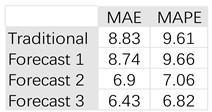
The SD, EOL, and MAE as calculated by the decision-machine and the comparison to traditional methods are shown in Table 3; the MAE and MAPE of the traditional methods, and three forecasts produced by the decision-machine are shown in Table 4.
In Table 3, the of 4.26 is less than the traditional methods of 5.73; where the consistency conditions are met by the outputted in (21); in which the SD is 0.86 and the EOL is 0.42.
In Table 4, the average MAE and MAPE of the three decision-machine’s predictions are 7.35 and 7.84 respectively, both better than traditional methodology’s MAE of 8.83 and MAPE of 9.61.
As seen in Table 1, the four values highlighted in red reflects the four incorrect “guesses” made by the decision-machine; where the probability that the decision-machine “believes” the entity moves upwards is 54% on average; the probability that it “believes” the entity moves downwards is 49% on average; which leads to a slight increase in the average produced shown in Table 2.
In Table 2, the average of 1000 forecasts produced by the decision-machine as shown in the Average column is fairly close to the mean of 106 produced by traditional methods, which shows that the decision-machine’s produced results encompass those of traditional statistical ensemble results.
When it comes to describing phenomena engaged in a random walk, traditional methods resort to using a statistical ensemble – attempting to produce a forecast for a single event is completely given up and only a probability distribution of where an entity might be is produced. By applying our methodology, the decision-machine is able to produce a forecast of the trajectory of a single event.
We’d like to emphasize that a so-called effective forecast of the future doesn’t necessarily always mean it is an accurate forecast, because no one can predict what will happen in the future; an effective prediction is just means of one that complies with a consistent rule of induction, in which it performs reliable and reasonable predictions; the accuracy of a prediction can only be evaluated until after what it attempted to predict has actually happened, in which the original prediction is then compared to the actual event.
9. Conclusions
We have developed a framework for the decision-machine to conduct scientific discovery automatically as an operator operation, evaluation, and optimization. Our proposed framework consists of three distinct parts: (1) an abstract formalism is the logic skeleton of the decision-machine to perform “deductive inference”; (2) the correlation between the abstract formalism and the observable phenomena is expressed by the three inductive rules; (3) the evolutionary algorithm is used to optimize the process of scientific discovery conducted by the decision-machine.
Using the example of a completely random-walk like one dimensional time series dataset, the decision-machine is able to geometrically reconstruct any curve and effectively predict its future by self-learning and self-adapting with the evolutionary algorithm. Furthermore, compared to traditional methods, the decision-machine doesn’t attempt to describe nature fully in terms of differential equations and don’t rely on statistical ensembles, and are able to produce single-event forecasts.
Future studies will include expanding our decision-machine to other real-world datasets in the natural and physical sciences.
Lastly, we are not attempting to create a fully perfect omnipotent machine to accurately predict the future, but rather a self-learning and self-adapting machine to “deal with” nature’s creative evolution that can cope with the problems that even the machine designer cannot foresee.
Scientific discovery isn’t just about backtracking the past and to predict the future but more importantly it’s about challenging the uncertain, ever-changing, modifiable nature. We shouldn’t naively believe that nature is static and there is some simple final structure “sitting” somewhere for us to find, scientific discovery is more about finding the unknown of the unknown.
Data Availability Statement
The authors confirm that all data generated are included in the manuscript. Data is available upon request from the corresponding author K. X. on reasonable request.
Acknowledgments
This work received no funding.
Conflicts of Interest
The authors declare that they have no conflicts of interest regarding the publication of this paper.
References
- Kuhn, T. S. (1973). The structure of Scientific Revolutions Thomas S. Kuhn. Univ. of Chicago Press.
- Popper, K. R., & Freed, J. (1959). The logic of Scientific Discovery: Karl R. popper. Hutchinson.
- Strevens, M. (2022). The knowledge machine: How an unreasonable idea created modern science. Penguin Books.
- Mach, E. (2019). Science of Mechanics: A Critical and historical account of its development. Forgotten Books.
- Whitehead, A. N. (1957). The concept of nature. University of Michigan Press.
- Strogatz, S. (2020). Infinite powers: How calculus reveals the secrets of the universe. Houghton Mifflin Harcourt.
- Von Neumann, J. Mathematical Foundations of Quantum Theory, Princeton, NJ: Princeton University Press (1932).
- Jammer, M. The Philosophy of Quantum Mechanics, New York, NY: John Wiley & Sons (1974).
- Dirac, P.A.M., the Principles of Quantum Mechanics, Oxford University Press (1958).
- Heisenberg, W., the Physical Principles of the Quantum Theory, Chicago, IL: The University of Chicago Press (1930).
- Xin, L., Xin, H. Decision-making under uncertainty – a quantum value operator approach. Int J Theor Phys 62, 48, https://doi.org/10.1007/s10773-023-05308-w (2023).
- Xin, L.; Xin, K.; Xin, H. 2023 On Laws of Thought—A Quantum-like Machine Learning Approach. Entropy, 25, 1213. (doi:10.3390/e25081213).
- Xin, L. Z., & Xin, K. (2025). Is the Market Truly in a Random Walk? Searching for the Efficient Market Hypothesis with an AI Assistant Economist. Theoretical Economics Letters, 15, 895-903. https://doi.org/10.4236/tel.2025.154049.
- Xin, L. Z.; Xin, H. 2022. Quantum Measurement: A game between observer and nature? https://doi.org/10.48550/arXiv.2210.16766.
- Xin, L.; Xin, K. 2025. AI Assistant Scientist: Aiding scientific discovery with quantum-like evolutionary algorithm. https://doi.org/10.51094/jxiv.1103.
- Devlin, K. J. (2010). The unfinished game: Pascal, Fermat, and the seventeenth-century letter that made the World Modern. Basic Books.
- Savage, L.J.: The foundation of Statistics. Dover Publication Inc., New York (1954).
- Feynman, Richard Phillips. (1967). The character of physical law. MIT. Press.
- Holland, J., Adaptation in Natural and Artificial System, Ann Arbor, MI: University of Michigan Press (1975).
- Koza, J.R., Genetic programming, on the programming of computers by means of natural selection, Cambridge, MA: MIT Press (1992).
- Koza, J.R., Genetic programming II, automatic discovery of reusable programs, Cambridge, MA: MIT Press (1994).
Figure 1.
Fitting results graph produced by the decision-machine.
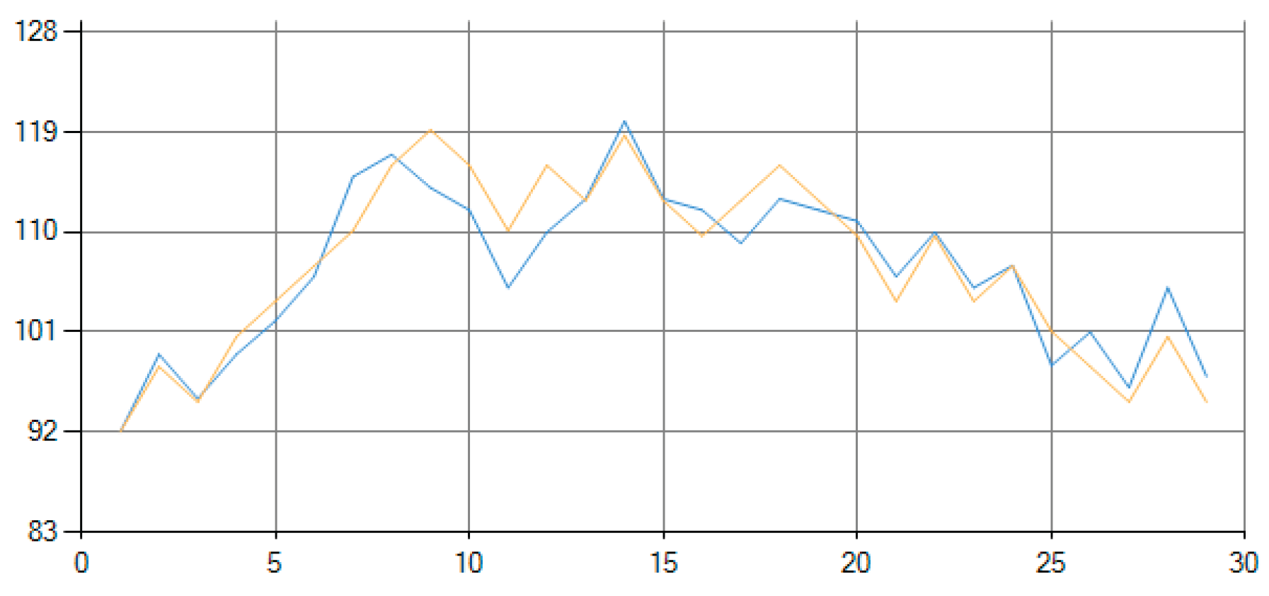
Figure 2.
The three predictions (a)-(c) produced by the decision-machine; (a) Forecast 1; (b) Forecast 2; (c) Forecast 3.
Figure 2.
The three predictions (a)-(c) produced by the decision-machine; (a) Forecast 1; (b) Forecast 2; (c) Forecast 3.
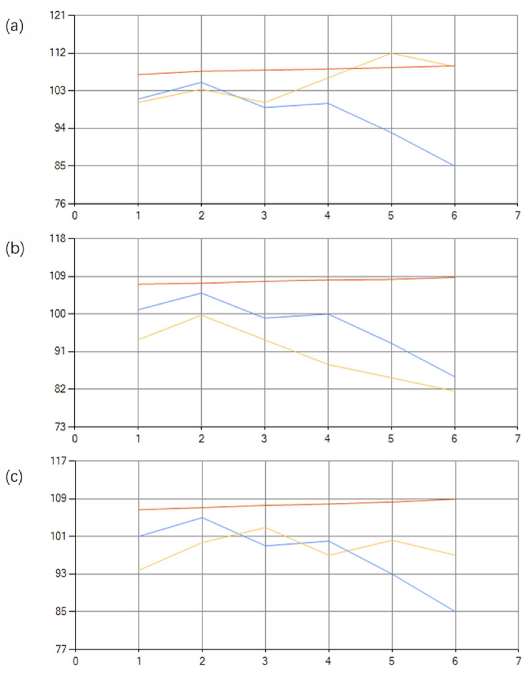

Table 1.
Numerical fitting results produced by the decision‐machine.
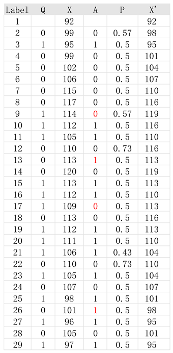 |
Table 2.
Results of the verify dataset.
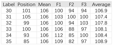 |
Table 3.
Evaluation metrics of the fitting results.
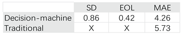 |
Table 4.
MAE and MAPE of traditional methodologies and three decision‐machine predictions.
 |
Disclaimer/Publisher’s Note: The statements, opinions and data contained in all publications are solely those of the individual author(s) and contributor(s) and not of MDPI and/or the editor(s). MDPI and/or the editor(s) disclaim responsibility for any injury to people or property resulting from any ideas, methods, instructions or products referred to in the content. |
© 2025 by the authors. Licensee MDPI, Basel, Switzerland. This article is an open access article distributed under the terms and conditions of the Creative Commons Attribution (CC BY) license (http://creativecommons.org/licenses/by/4.0/).
Copyright: This open access article is published under a Creative Commons CC BY 4.0 license, which permit the free download, distribution, and reuse, provided that the author and preprint are cited in any reuse.


