
Submitted:
12 September 2025
Posted:
15 September 2025
You are already at the latest version
Abstract
Oil content (OC) and protein content (PC) are two important traits determining the quality and yield in soybean. However, these traits are quantitative in nature, governed by polygenes possessing minor effects. In this study, we performed multi-locus genome-wide association studies (GWAS) to identify the quantitative trait nucleotides (QTNs) associated with OC and PC by using the 4404 multiparent F4 individuals genotyping with 20K SNP chip. A total of 83 and 110 QTNs significantly associated with OC and PC, respectively were detected by using six multi-locus GWAS methods. The identified QTNs as well as genome-wide SNPs (9,942 SNPs) were tested with training populations (TP) of different sizes for genomic selection (GS) analysis. Our results revealed that using the QTNs only has allowed to provide the higher prediction accuracy of 0.70 at reduced TP size of 10%; besides, using the QTNs-specific to each trait viz., OC and PC for GS selection minimizes the negative correlations among these traits. The present study, provided the detailed genetic architecture of PC and OC in soybean, besides provided a new method for developing soybean cultivars with both high PC and OC, which otherwise was the long-term unachievable goal of the soybean breeders.
Keywords:
soybean
; genomic selection
; quantitative trait nucleotides
; quality
; protein
; oil
1. Introduction
Soybean (Glycine max L.) is cultivated globally as an important cash crop, which is largely attributed to the fact that soybean seeds are rich in edible protein and oil. In soybean, the average seed protein content (PC) is 42.1%, and the average oil content (OC) is 19.5% [1]. According to statistics of the USDA, it has been estimated that soybean account for about 68% of world protein consumption, and 57% of world oilseed production [2]. Soybean is the main source of edible oil, and soybean protein contains all essential amino acids for human health [3]. Therefore, it is vital to develop soybean cultivars with high OC and PC; hence, these traits are the major and core objectives of the soybean breeders across the world [4,5].
Both PC and OC are complex quantitative traits that are controlled by polygenes possessing low heritability and high environmental influence [6,7]. Although, hundreds of QTLs/genomic loci associated with the OC and PC in soybean has been reported and documented in the SoyBase (http://www.soybase.org). Most of these QTLs has not been confirmed as well as utilized in soybean breeding [8]. The main reason was the low resolution of early mapping approaches, as well as limited genetic diversity used in the gene mapping [8]. Furthermore, mapping studies carried out earlier for both quality traits in soybean were mainly based on the identification of major-effect QTLs, and negligible efforts have been made on the study of complex genetic effects such as epistasis and environment effects [9]. In contrast to classical linkage mapping, a genome-wide association study (GWAS) uses broader genetic diversity for gene mapping and is based on linkage disequilibrium (LD) exhibited high mapping resolution and abundant genetic variation due to the high recombination events in diverse populations. The GWAS has been efficiently used to identify the QTLs/genes underlying the various yield-related traits in soybeans such as PC and OC [10], agronomic traits [11], salt tolerance [12] and other yield-related traits [13]. In recent years, genomic selection (GS) based on a large number of molecular markers is a potentially effective breeding improvement method for complex quantitative traits controlled by multiple genes in plants [14]. Various GS models have been developed, including direct methods such as GBLUP [15], ssBLUP [16,17], sBLUP, and cBLUP and indirect methods such as rrBLUP [21] , BayesA and BayesB [22], BayesCπ and BayesDπ [23] and Bayesian LASSO [24]. The main difference between these models is the assumption of a marker effect that affects the total variance. Previous studies have shown that different models may have different prediction effects for different traits [25,26].
Although GS is relatively mature in the algorithms of the model, the application of GS in commercial plant breeding is limited by two main factors: (i) genotyping costs; and (ii) unclear guidelines as to how GS can be efficiently applied in a breeding program [27,28,29,30]. The size of the training population (TP) and the marker number are the key factors regulating the genotyping cost as well as the GS prediction accuracy [31]. There are many studies that tried to reduce the genotyping cost of GS by reducing the number of markers, especially in the case of animals, and reported well prediction accuracy [32]. However, for annual crops, the genotyping cost of even several thousand markers would make GS lose its advantage in cost due to the extremely low individual unit price. Therefore, strategies of GS selection using low-density markers need to be explored in plants.
In breeding programs, breeders simultaneously carry out selection for multiple traits; however, there are many traits that show genetic correlation to each other, and this correlation can be either among the desirable traits or between desirable and undesirable traits. In this regard, the OC and PC in soybean are well known and documented to show a negative correlation, and the relevant functional genes had opposite effects on the two traits [33,34]. For antagonistic traits, the selection of one trait tended to result in the decline of the other [35,36]. Understanding the detailed genetic architecture of these traits at the high resolution will assist to minimize this negative correlation among these traits to a greater extent [8]. For example, in the case of improving the flavor of tomatoes, the loci only related to the content of metabolites were selected, whereas no loci have been selected that could increase the sugar content while having a negative effect on yield; and by following this strategy it was possible to improve the flavor of fruits without having the negative effect on yield [37].
In this study, our main objectives were: (1) to identify the quantitative trait nucleotides (QTNs) associated with OC and PC in soybean via GWAS; (2) to evaluate the differences in prediction accuracy for OC and PC by using different GS models; (3) to access the feasibility in prediction accuracy by reducing the TP size and incorporating only QTNs markers in the GS model, that might providing a basis for further cost reduction in subsequent GS applications; and (4) utilizing only trait-specific QTNs in the GS for minimizing/breaking the negative correlation among the PC and OC traits; thereby improved the efficiency for simultaneously increasing the antagonistic traits of OC and PC. In the current study, by using the six different multi-locus GWAS methods, we identified a total of 83 and 110 QTNs significantly associated with OC and PC, respectively. To this end, we used these identified QTNs and genome-wide SNPs to construct TP in different proportions for GS analysis. Our study reported that an economical and practical prediction accuracy of 0.70 can be achieved by using minimum TP (10%) and fewer markers (83 or 110 QTNs) for simple genetic backgrounds. Hence, reduced TP size corresponding to the high prediction accuracy can be attributed due to the use of QTNs in the GS analysis. Therefore, it provides the best strategy to reduce the cost of the GS analysis, which is a major challenge for the commercial utilization of GS in the crop improvement. Besides, our study documented that GS allows for improving the PC by using the PC-specific QTNs without having any considerable influence on its highly negatively correlated trait OC and vice-versa. This provides preliminary evidence that genomics-assisted breeding has the potential to improve simultaneously the negatively correlated desirable traits. Hence, provide a novel strategy for the simultaneously breeding of negatively correlated traits in soybean.
2. Results
2.1. Phenotypic Characterization of Multiparent F4 Population
In the current study, we used the 4,404 soybean genotypes derived from six F4 single-hybrid populations (Table S1). The six populations were developed from six different bi-parental crosses involving three male parents and four female parents (Table S1), and the semi-sib relationship was prevalent among the populations. The agronomic performance of quality-related/yield-related traits of these parents are presented in Table S1. Moreover, the two traits viz., OC and PC showed approximately normal distribution in all six F4 segregating plus combined populations (Figure 1, Figure S1 and Table S1). In the case of OC, the average value of OC for F4GS3 was the highest (20.56%), and that of F4GS4 was the lowest (18.05%). The standard deviation of OC in different populations was also different, among which the standard deviation of F4GS1 was the highest (1.14%), and that of F4GS2 has the lowest (0.94%). Among the PC values, the average value of F4GS5 was the highest (43.58%), while F4GS3 has the lowest (39.15%). Within each population, the standard deviation of PC also varies. The standard deviation of F4GS1 was the highest (2.08%), and that of F4GS5 has the lowest (1.68%). In addition, we found that OC and PC exhibited a negative correlation in each population, with the Pearson correlation coefficient ranging from -0.76 to -0.86 (Table S1). This is consistent with previous reports [34].
2.2. Population Structure Analysis
In this study, we genotyped the soybean population using a customized soybean genotyping panel. The custom panel contained a total of 20,659 SNP markers mainly derived from the genic/protein-coding regions of the soybean genome. By using the quality control filtering, we retained a total of 9,942 high-quality SNPs, that were used for the further genetic analysis. For these 9,942 SNP markers, we estimated the markers density as the number of SNPs per 1Mb contiguous window in the soybean genome (Figure 2A). Our results showed that these SNP markers covered almost the whole soybean genome. However, the markers located near the telomere region were relatively dense, while the markers located around the centromere were relatively scarce, which was consistent with the gene distribution in the soybean genome [38].
To study the genetic structure of six populations, we carried out the phylogenetic analysis and PCA analysis. Results of the phylogenetic analysis showed that individuals from the same single hybrid combination are clustered together in the phylogenetic tree. However, the F4 populations possessing one parent in common are clustered near each other in the phylogenetic tree (Figure 1C). To this end, PCA results also showed that individuals from the same population are obviously clustered together, but the population distribution areas of half-sib families are closer and overlap with each other, such as “F4GS1 and F4GS2” & “F4GS3 and F4GS4”. Hence, the results of both phylogenetic analysis and PCA are consistent with each other (Figure 1D). Besides, our results revealed that these six F4 populations are different genetically with some relatedness.
2.3. QTN Identification for OC and PC Traits via GWAS Analysis
To use reduced markers number with higher prediction accuracy in GS, we performed the GWAS analysis in the whole populations (i.e., a combination of six populations consisting of 4,404 lines) to detect QTNs associated with the OC and PC; and subsequently, these QTNs were used for the GS analysis. We adopted six different multi-locus association analysis algorithms/models viz., FASTmrEMMA, FASTmrMLM, ISIS EM-BLASSO, mrMLM, pKWmEB, and pLARmEB to improve the power of QTNs detection. Eleven to forty-one QTNs linked with OC were detected through these six different models (Figure 2B & 2C; Table S2). Fifty-eight OC QTNs were only detected by one model, while twenty-five OC QTNs were detected by at least two or more models. Finally, the same QTNs detected by different algorithms were de-redundant, and 83 OC QTNs were retained (Figure 2B, Table S2), which were located on all chromosomes except chromosome 13. The phenotypic variance explained (PVE) by OC QTNs ranged from 3.75×10-08% to 7.80%. For the case of PC, ten to forty-nine PC QTNs were detected from different algorithms. Forty-two QTNs were detected by at least two or more algorithms. Finally, a total of 110 PC QTNs were retained after de-redundancy (Figure 2C, Table S2), which were located on all chromosomes except chromosome 11. Phenotypic variance explained by PC QTNs ranged from 1.29E-08% to 9.56%.
Next, we compared the location of OC and PC QTNs on the soybean chromosomes. Among these two QTNs sets (viz., OC and PC), a total of 25 QTNs’ positions were completely overlapping, and these 25 QTNs represent the common QTNs for both OC and PC traits. These 25 QTNs had completely opposite effects on the OC and PC traits (Table S2). Furthermore, we relaxed the criteria to classify the two sets of QTNs with distances less than 1Mb as overlapping QTNs. Under this criterion, only 37 of the 83 (44.6%) OC QTNs were OC-specific QTNs, and the remaining 46 (55.4%) were overlapped with PC QTNs. Only 62 of the 110 (56.4%) PC QTNs were PC-specific QTNs, and the remaining 48 (43.6%) were overlapping with OC QTNs. These results indicated that a large number of QTNs controlled both OC and PC traits simultaneously, but these common QTNs showed contrasting effects on both traits confirming their negative correlation at the genetic level.
2.4. Effect of Model Selection on GS Prediction Accuracy
Prediction accuracy of six different GS models viz., Bayes A, Bayes B, Bayes C, Bayesian Ridge Regression, Bayesian Lasso and RRBLUP were evaluated in this study. Prediction accuracy was assessed using a 10-fold cross-validation method to assess the correlation between predicted and actual values. The average prediction accuracy of Bayes A, Bayes B, Bayes C, Bayesian Ridge regression, Bayesian Lasso, and RRBLUP for OC is 0.749, 0.735, 0.748, 0.750, 0.733, and 0.731, respectively (Figure 3A). There was no significant difference among the different models on the prediction accuracy (for this we used the Least Significant Difference test,P value > 0.05). The average prediction accuracies for PC content were 0.756, 0.764, 0.756, 0.756, 0.757, and 0.763, respectively; and there was also no significant difference among the different models (Least Significant Difference test,P-value > 0.05) (Figure 3B).
We further evaluated the differences in prediction accuracy between the different models using only QTNs markers i.e., 83 OC QTNs for OC prediction, and 110 PC QTNs for PC prediction. The average prediction accuracy of Bayes A, Bayes B, Bayes C, Bayesian Ridge Regression, Bayesian Lasso, and RRBLUP for OC were 0.747, 0.753, 0.761, 0.749, 0.753, and 0.755, respectively (Figure 3A). The average predictive accuracy for PC were 0.777, 0.764, 0.765, 0.778, 0.772, and 0.778, respectively (Figure 3B). Our results showed no significant differences in the prediction accuracy of GS models for the two traits. The above result indicated that different GS models had similar prediction ability for both traits whether using all the markers or the QTNs markers only. Therefore, we selected rrBLUP, which is the fastest running model, for our subsequent GS study.
2.5. Effect of TP Size and Marker Number on GS Prediction Accuracy
Size of TP and number of genotyping markers are the main components determining the cost for GS application. Therefore, we further tried to reduce these two factors by evaluating their effects on the GS accuracy of soybean for OC and PC. Based on the rrBLUP model with genome-wide SNPs markers, the proportion of TP increased from 10% to 90% of the whole population, the prediction accuracy for OC increased by 0.054 from lowest (0.687) to highest (0.741), respectively (Figure 4A, Table S3). Prediction accuracy for PC increased by 0.064 from the lowest value (0.698) to the highest value (0.762). The prediction accuracy of the two traits presented a significant upward trend with the expansion of the TP size, until the TP size reached 70%–80% of the whole population (Table S3). To this end, we also evaluated the accuracy of GS prediction for different TP sizes using only QTNs markers. We observed that the prediction accuracy for OC also tended to increase gradually while only increasing 0.040 from the lowest value (0.721) to the highest value (0.761) (Figure 4B, Table S3). Prediction accuracy for PC also showed a gradual increase from the lowest value (0.746) to the highest value (0.772) with only increasing 0.026. Hence, our results revealed that compared to genome-wide SNPs markers used in the GS of OC and PC, the prediction accuracy of GS modeling using QTNs markers tended to increase more gently with the increase in population size. This indicates that using the QTNs will allow to provide higher prediction accuracy even at lower TP size.
Furthermore, we also compared the GS predictions accuracy using two marker sets (genome-wide SNPs markers vs QTNs markers) under the same TP size. When the TP size was small, the GS model based on QTNs only (hereinafter referred to as GSQTN model) was significantly superior to the GS model based on all markers (hereinafter referred to as GSall model). However, the dominance of GSQTN model decreased with the increase in TP size (Figure 4). Therefore, when the TP size reached 80–90% of the whole population, there was only a slightly significant difference or even no significant difference between GSall and GSQTN models. This also suggests the use of QTNs in GS will allow to use lower TP size with higher prediction accuracy.
2.6. Effect of Trait Specific QTNs on GS Prediction Accuracy
There was many common QTNs between OC and PC, and the effects of common QTNs on the OC and PC were in the opposite direction. Therefore, the selection of these QTNs led to the improvement of one trait at the cost of a decrease in the other correlated trait. Hence, we attempted to predict two traits using trait-specific QTNs i.e., 37 OC-specific QTNs, and 62 PC-specific QTNs. The results showed that although the number of trait-specific QTNs was only 44.6% and 56.4% for the OC and PC, respectively, and the prediction accuracy using trait-specific QTNs could generally reach the level of 0.70 (Figure 5).
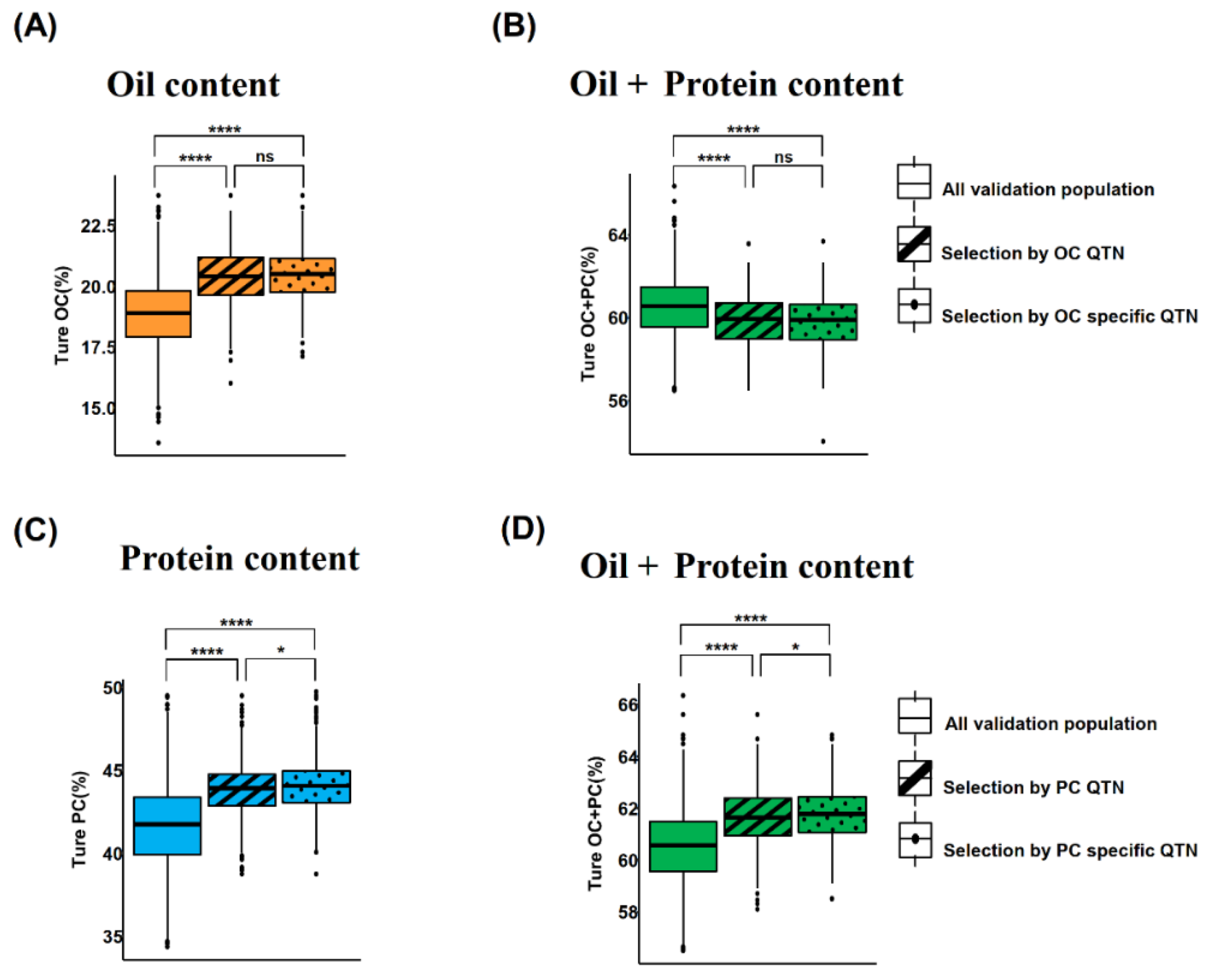
To minimize the negative correlation between OC and PC, we follow a strategy of using trait-specific QTNs of OC and OC in GS analysis. We randomly selected half individuals as TP, and the remaining half as validation population (VP). Firstly, OC was predicted using OC-specific and all OC QTNs in TP; then two subgroups present in the top 20% of predicted OC values were selected from VP, respectively. The average OC values of the two subgroups showed a non-significant difference (Figure 5A); but their OC values were significantly higher than the average OC value of the whole VP (Figure 5A). As the OC QTNs also include OC-specific QTNs besides the common QTNs in the GS prediction, this indicated that common QTNs only had limited contribution for OC prediction. In contrast, OC + PC values of two subgroups were remarkably reduced relative to VP (Figure 5B), indicating negative correlation among OC and PC. While the two subgroups showed a non-significant difference. Moreover, PC was also predicted based on PC-specific QTNs and all PC QTNs, respectively; and two subgroups in the top 20% of predicted PC values were selected. The average PC of the subgroup selected by PC-specific QTNs was significantly higher than the average PC of the subgroup selected by PC QTNs (P = 0.018) (Figure 5C); their average true PC values were significantly higher than the whole VP. The average true PC + OC values of the two subgroups significantly increased relative to VP (Figure 5D). Moreover, the average PC + OC of the PC-specific QTNs-screened subgroups was significantly higher than all PC QTNs-screened subgroups (P = 0.013) (Figure 5D). In total, our results showed that the use of trait-specific QTNs had potential ability to minimize negative correlation among OC and PC; thus, providing an alternative method for simultaneous improvement of both OC and PC in the same soybean cultivar if a larger number of the OC-specific and PC-specific QTNs are available.
3. Discussion
3.1. Effect of GS Models on Prediction Accuracy
GS method allows the selection of desirable plants for crop traits (that appears at the maturity stage) at the seed or seedling stage, which not only effectively shortens the breeding cycle, but also reduces the breeding cost; hence, GS has emerged as an important approach of genome-assisted breeding (GAB). Different GS models are based on different hypotheses involving varied QTL effects distribution characteristics [39]. For example, rrBLUP assumes that QTL effects are in accordance with the normal distribution [21, Bayes A assumes the QTL effects are in accordance with the t-distribution [22] and Bayesian LASSO assumes the QTL effects are in accordance with the double exponential distribution [24]. Theoretically, for different types of traits and populations with different genetic structures, the optimal GS model in a specific situation needs to be confirmed through a pilot study [40]. However, in the current study, we want to understand whether GS predictions are affected by using either all genome-wide SNPs markers or only QTNs markers; besides, did the prediction accuracy of different GS models reveal any significant or non-significant differences. Our results confirmed non-significant difference between the different GS models on the prediction accuracy for OC and PC traits. These results are contrasting as observed in soybean for chlorophyll content associated with cyst nematode tolerance [41], and for eight agronomic traits in chickpea [42]. This might be due to the limited genetic diversity of the F4 population derived from seven different parents that are used in the current study. Therefore, we selected rrBLUP as the main analysis model; because, in this model, the marker effect is assumed to follow a normal distribution, whereas all effects are shrunken to a similar and small size [43]. By considering the QTNs effect estimated by multi-locus GWAS (Figure S2), it has been observed that QTNs effects did not conform to the typical normal distribution but present a bimodal distribution. The main reason is that QTNs with too weak/minor effects were undetectable (not significant) via GWAS analysis. Therefore, GWAS analysis cannot identify the QTNs associated with the trait of interest with a very minute effect even approaching to near zero. Based on the results of rrBLUP analysis using QTNs, the distribution of QTNs predicted effects also presented a bimodal distribution, while the predicted effects were generally closer to zero (Figure S2). Therefore, there was a significant difference between the distribution of QTNs effects estimated by GWAS and GS. However, relevant studies have shown that in the high-dimensional regression used by GS prediction, different methods could have great differences in estimating the values of SNPs markers effects but may obtain similar overall prediction accuracy. In a simulation study [44], although the correlation between the estimated markers effects of Bayesian ridge regression and BayesA was low (0.226), the correlation between phenotypic predictions from the two models was as high as 0.946. Therefore, for GS studies, good prediction accuracy can be achieved even though different models with different assumptions about the distribution of marker effects. The assessment of model suitability only needs to focus on the accuracy of trait prediction, rather than whether the model's assumption of marker effects is correct.
3.2. Elucidating Effect of TP Size and Markers Number on GS
GS provides an alternative to the traditional soybean breeding method which mainly relies on phenotypic selection and uses genetic information to make breeding decisions. Controlling the cost of GS is a key factor affecting its commercial application in crop improvement. Every step of the GS approach is a potential entry point for regulating the cost of GS cost. These steps include reducing the cost for DNA extraction and sequencing, designing an effective TP with minimal size, fast and accurate phenotypic measurement of the TP, and reducing the cost of genotyping. In this study, we found that by using only 10% of individuals (about 440 individuals) from the whole population (4404), prediction accuracy of 0.687 and 0.721 could be obtained for the two traits viz., OC and PC, respectively. Previous studies have documented that GS with a prediction accuracy of only 0.50 can also result in two-fold higher genetic gain per year compared to traditional MAS in a low-investment wheat breeding program (h2 = 0.13), and a three-fold hike in a high-investment maize breeding program (h2 = 0.11) [45]. Of course, the relatively simple genetic diversity of our population might reduce the requirement for TP size. In subsequent studies, we will test the need of TP size for GS in the context of more complex genetic diversity.
The number of markers is also a key factor affecting the cost of GS applications. In this study, we used a custom-designed 20k chip. The cost of genotyping was as high as 120 ¥/ plant at 20k chip, which was higher relative to the cost of planting one soybean, and performing OC and PC phenotypic assays [46]. Thus, reducing genotyping costs is the key factor for the practical and commercial application of GS in crop breeding. In this study, we found that the GSQTN model using only 83 and 110 QTNs associated to OC and PC, respectively could achieve higher prediction accuracy than GSall model based on all markers. There are two key factors affecting the prediction accuracy of GS. First, markers could cover most of the effective chromosomal regions. Second, the effect of markers can be correctly fitted into the model. The proportion of phenotypic variance explained (PVE) by the GSall model in this study were 32.97% (OC) and 38.38% (PC), while the proportions of PVE by GSQTN models with fewer markers could reach to 23.67% (OC) and 23.06% (PC) (Table S3). This can be explained as, the GWAS models cannot detect the QTNs with minute effect on the trait of interest, whereas the GS models can fix all the genetic variation governed even by QTNs with minute effect on the trait. Hence, this is the reason why the GSall model fixes more PVE for the OC and PC traits compared to GSQTN models. In addition, the TP size requirement for GSQTN modeling is lower. The advantage of the GS model is that it can fit the effects of markers (as independent variables) even though the number of markers is much larger than number of individuals (phenotype of individuals as dependent variables). However, the addition of a larger number of markers would greatly increase the computational complexity of the regression model of GS, and a larger TP would be required to accurately fit the effects of the markers [47,48,49]. The use of several hundred to a thousand markers in the GWAS analysis of Asian rape has been reported to provide higher prediction accuracy compared to a high-density array in breeding populations with strong linkage disequilibrium [50]. Besides, 500 markers or less are selected by GWAS of Phytophthora sojae resistance to conduct GS, and the predictive ability was comparable to GS using 33,000 markers [51]. These previous studies have demonstrated that reducing the markers density through pilot studies such as GWAS, is a promising approach in reducing the cost of genotyping with concurrent high prediction accuracy in GS. In this study, with the continuous expansion of the TP size, the prediction accuracy of the GSQTN models was significantly higher than GSall models; besides, when the TP size is increased beyond 30%, there is no significant increase in the prediction accuracy with the increase in TP size. These results showed the use of QTNs in the GS models will provide greater prediction accuracy even at lower TP size, thus providing the best alternative to reduce the cost of conducting effective GS analysis.
In this study, we observed that prediction accuracy using GSQTN model was higher that too at the smaller TP size. However, GSQTN model means that pilot GWAS needs to be conducted for different traits in different populations, before designing custom QTNs chips. Pilot GWAS will involve additional time and experimental costs. Moreover, QTNs markers integration for multiple traits may increase the markers density and cost of the custom chip. With the cost of genotyping still relatively high at the present stage, it is still a relatively pragmatic strategy to design QTNs chips for a small number of key traits [46]. If the genotyping cost continues to decline in the future, the GS using genome-wide covered chips can be considered, thus realizing the GS for various populations and traits without the need for customized chips.
3.3. Genomics Selection for Antagonistic Trait
In this study, we found that large numbers of common QTNs controlled both OC and PC; and the effects of these QTNs on the OC and PC traits were in opposite directions. This further explained the strong negative correlation between these two seed traits. These common QTNs with opposite effects might exist because of two mechanisms viz., pleiotropy and linkage [52]. In the case of pleiotropy, the QTN locus is located within a single functional gene, and the function of this gene itself has a desirable and undesirable effect on the two correlated traits such as OC and PC. For example, a QTN allele could increase OC but lead to a decrease in PC. In the second case i.e., linkage, there are two or more functional genes strongly linked in a particular locus, and the functional effects of these genes on the two traits will be opposite for the two traits such as OC and PC. However, the negative correlation existing among the two traits such as OC and PC because of pleiotropy is impossible to break; therefore, restricts the simultaneous increase of the OC and PC in soybean. Screening of such QTNs will inevitably reduce the value of a trait when another trait is improved. However, negative correlations existing because of the linkage of genes can be broken by increasing population size and creating new recombination’s [53]. Thus, it allows to simultaneously increase the correlated traits, but it costs higher breeding costs. To this end, our study revealed that by using the trait-specific QTNs, the breeding of a trait i.e., OC that is negatively correlated with PC can be achieved with less interference on the decrease of the PC and vice-versa. This provides the novel strategy to simultaneously increase the PC and OC traits in the soybean cultivar, which otherwise is a long-term goal/objective of the soybean breeders and was impossible to achieve via conventional breeding approaches. Hence, this approach will allow use of GS successfully in the improvement of mutually exclusive traits in the future. However, for its practical utility, it needs some more verification by using more diverse population in soybean as well as validate this approach in different crop species for different types of negatively correlated traits. In this way, we will be successful to develop soybean cultivars with both high PC and OC.
4. Materials and Methods
4.1. Plant Materials
Seven soybean cultivars viz., FNGS0852, FNGS0225, FNGS0239, FNGS0217, FNGS0256, FNGS0280 and FNGS0301 collected from northeast China were used to construct six single-hybrid F4 populations (Table S1). The PC and OC of these seven cultivars are; FNGS0852, PC =44.64% & OC = 19.35%; FNGS0225, PC = 40.95% & OC = 21.60%; FNGS0239, PC = 43.46% & OC = 19.67%; FNGS0217, PC = 40.72% & OC = 22.01%; FNGS0256, PC = 44.35% & OC= 20.94%), FNGS0280, PC = 44.84% & OC = 18.52%; and FNGS0301, PC = 46.69% & OC = 17.90%. The population size, pedigree relationships and parental agronomic characteristic of these six F4 bi-parental populations viz., F4GS1, F4GS2, F4GS3, F4GS4, F4GS5 & F4GS6 are presented in Table S1. The single seed descent (SSD) method was followed for the development of these populations. All the six population along with their parents were planted in the experimental farm of the Jiamusi Branch of Heilongjiang Academy of Agricultural Sciences, Jiamusi, Heilongjiang, China. These population were planted in a single-line plot of 1 m in length and 0.5 m in width; and the standard cultural and agronomic practices were followed to grow these populations.
4.2. Phenotype Data Collection and Analysis
The seed samples collected were placed in a cup with a bottom of 5cm in diameter, and a height of 3cm for near-infrared spectroscopy analysis; and the seeds were analyzed without any treatment and in good condition. The cup is filled with the equivalent of about 60ml of soybean seed (about 20 g or 80 seeds). Spectra acquisition was performed with a Fourier transform near-infrared (FTNIR) analyzer (Antaris II spectrometer: Thermofisher Scientific, France). Spectra were collected in reflectance mode with an 8 cm-1 optical resolution and were obtained as an average of 64 scans. Besides, the spectra were collected over the range of 4000 to 10000-1, and calibrations were done using four spectral ranges: from 4100 to 4940 cm-1; from 5390 to 6690 cm-1; from 6900 to 7130 cm-1; and from 7185 to 9000 cm-1. These spectral regions provide useful information about the crude PC as well as crude OC of the soybean seeds, and excluded the water spectral regions. They have been selected by looking at the regression vector from the Partial least square method (see Development of NIRS Calibration Models) and Thermo proprietary pure component algorithm. Lastly, the OC and PC are expressed in percentage by weight of seeds.
The distribution probability density map of OC and PC is constructed by using the R package ggpubr (https://cran.r-project.org/web/packages/ggpubr/index.html). The descriptive statistics of phenotypic data are carried out by "describe.by" of R package psych(https://cran.r-project.org/web/packages/psych/index.html). Pearson correlation coefficient (r) is calculated by using the "cor" function implemented in the R package psych.
4.3. Genotyping Analysis
Total genomic DNA was extracted by the hexadecyl trimethyl ammonium bromide method from the young and fresh leaves of each soybean genotype [54]. The 20K chip used in the present study for the genotyping was developed by MOLBREEDING Biotechnology Company (Shijiazhuang, China). A total of 20,000 SNP markers of the 20k Chip were selected from whole-genome sequencing data of 270 varieties selected from north China. The following criteria were used to select markers; (a) the deletion rate of all genotypes in the population should not exceed 20%, the proportion of heterozygous genotypes should not exceed 30%, and the allele frequency is between 5% and 95%; (b) Slide the window with the step size of 50 Kb, and select a marker for each window; (c) The markers located in the gene CDS region were selected preferentially. In the current study, the SNPs with secondary alleles frequencies (MAF)<0.05 and missing rate >10% were filtered out [4]. After quality filtration, a total of 9,942 SNPs were retained for further analysis.
4.4.Phylogenetic Relationship and Principal Component Analysis (PCA)
For inferring the genetic structure of the six bi-parental F4 populations, we performed the phylogenetic and PCA analysis by using the 9,942 SNPs markers. The phylogenetic tree is inferred by the maximum likelihood method (ML) of FastTree software [55], and the genetic diversity of all individuals is evaluated by visualization and editing in ggtree [56]. Population structure analysis based on principal component analysis (PCA) was executed in Plink software [57].
4.5.GWAS Analysis
The R package mrMLM (version4.02) was used to perform the GWAS. Six multi-locus GWAS methods within mrMLM were used to identify significant quantitative trait nucleotides (QTNs) associated with the OC and PC traits in soybean, that includes mrMLM [58], FASTmrMLM [59], FASTmrEMMA [60], ISIS EM-BLASSO [61], pLARmEB [62] and pKWmEB [63]. The critical P-value parameters for these methods at the first stage were set to 0.01 except for FASTmrEMMA, where the critical P-value was set to 0.005, and the critical LOD score was set to 3 for significant QTN at the last stage.
4.6. Genomic Selection
Genomic Selection modeling was implemented in the R (version 3.6.0) package BGLR [44], and R (version 3.6.0) package RRBLUP [22]. The genotypic effects were estimated by using the six statistical models including rrBLUP. This method assumed that all the genetic markers had effects on the target traits, and the effects of these markers followed the same normal distribution [21]. BayesA method assumes that all genetic markers have effects on the target trait, but their variances are not equal, but follow the inverse Chi-square distribution. BayesB method also assumed that the marker effect followed an inverse Chi-square distribution, but some markers were assumed to have zero variance, and BayesB assumed that a few large-effect loci controlled the target traits [22]. The purpose for the development of BayesCπ and BayesDπ is to solve the defect of BayesA and BayesB on the influence of prior hyperparameters, i.e., the uncertainty of QTL quantity controlling the target trait. The above two methods introduce a parameter π, which is an unknown prior probability that the SNP effect is zero. Compared with BayesDπ, the BayesCπ is sensitive to the number of simulated QTLs and the size of training data; and can provide information about genetic structure [23]. The Bayesian LASSO method assumes that the marker effects follow a double exponential distribution, and there is an exponential prior on the marker variances, resulting in more Shrinkage of large-effect markers and small-effect markers. Therefore, the presence of only a few markers with effect, and the comparison effect has a large influence. Bayesian LASSO method will get a better GS prediction effect [24]. In the BRR method, the effect factor vector is subject to gaussian prior, i.e., the effect vector of the predictor is subject to a normal distribution, and the coefficient compression effect generated by the prior assumption is similar to ridge regression [64]. The Least Significant Difference test and T-test were used to compare the prediction accuracy of different scenarios in R, and the significance was estimated at P > 0.05.
5. Conclusions
This study has achieved multiple preset objectives: successfully identifying QTNs associated with oil content (OC) and protein content (PC) in soybeans through genome-wide association study (GWAS); evaluating the differences in prediction accuracy for OC and PC among different genomic selection (GS) models; exploring the feasibility of reducing the size of the training population (TP) and incorporating only QTNs markers in the GS model on prediction accuracy, providing a basis for reducing costs in subsequent GS applications; and meanwhile, using trait-specific QTNs for GS to minimize or break the negative correlation between PC and OC, improving the efficiency of simultaneously improving these two antagonistic traits.
In this study, six different multi-locus GWAS models were used to identify 83 and 110 QTNs significantly associated with OC and PC, respectively. Based on these QTNs and genome-wide SNPs, TPs in different proportions were constructed for GS analysis. The results showed that for simple genetic backgrounds, an economical and practical prediction effect (correlation coefficient r > 0.7) could be achieved by using a minimum-sized (10%) TP and fewer markers (83 or 110 QTNs). It can be seen that the use of QTNs in GS analysis is an important reason for maintaining high prediction accuracy while reducing the TP size, which provides the best strategy for reducing the cost of GS analysis, and cost is a major challenge in the commercial application of GS in crop improvement.
In addition, the study confirmed that GS using PC-specific QTNs can increase PC without significant impact on OC, which is highly negatively correlated with it, and vice versa. This provides preliminary evidence that genomics-assisted breeding is expected to simultaneously improve negatively correlated desirable traits, and also provides a new strategy for the simultaneous breeding of negatively correlated traits in soybeans.
Supplementary Materials
The following supporting information can be downloaded at the website of this paper posted on Preprints.org, Figure S1. Figure S1. QQ plot of oil content(A) and protein content(B). The X-axis is the theoretical value under normal distribution, Y-axis is the actual value. Figure S2. QTN effect distribution detected by GWAS and QTNs effect distribution fitted by genomics selection with RRBLUP model; Table S1. Table S1. Six F4 populations derived from seven parents. Table S2 QTNs detected from GWAS. Table S3. Comparison of GS model prediction accuracy of soybean oil and protein contents with different maker types.
Author Contributions
Suxin Yang, Xianzhong Feng and Xiangfeng Wang conceived the study, designed and coordinated the training experiment. Guang Li and Huangkai Zhou completed statistical analysis of phenotypic data, contributed to development of GS protocols and wrote the paper. Kuanqiang Tang designed the field trials, statistically analysed phenotypic data. Jiantian Leng established field trials and statistically analysed phenotypic data. Suxin Yang, Javaid Akhter Bhat and Jiankang Wang wrote the grant and contributed to project execution.
Funding
This study was supported by the Biological Breeding-National Science and Technology Major Project (2023ZD0403201) and the National Natural Science Foundation of China (32201825).
Data Availability Statement
The original contributions presented in this study are included in the article. Further inquiries can be directed to the corresponding author.
Conflicts of Interest
The authors declare that they have no known competing financial interests or personal relationships that could have appeared to influence the work reported in this paper.
Abbreviations
The following abbreviations are used in this manuscript:
| OC | Oil content |
| PC | Protein content |
| QTNs | Quantitative trait nucleotides |
| GS | Genomic selection |
| TP | Training populations |
References
- Wilson, R.F. Seed composition. In Soybeans: Improvement, Production, and Uses; 2004; pp. 621-677.
- Zhang, J.; Song, Q.; Cregan, P.B.; Jiang, G.-L. Genome-wide association study, genomic prediction and marker-assisted selection for seed weight in soybean (Glycine max). Theor Appl Genet 2016, 129, 117–130. [Google Scholar] [CrossRef]
- Qin, J.; Shi, A.; Song, Q.; Li, S.; Wang, F.; Cao, Y.; Ravelombola, W.; Song, Q.; Yang, C.; Zhang, M. Genome wide association study and genomic election of amino acid concentrations in soybean seeds. Front Plant Sci 2019, 10, 1445. [Google Scholar] [CrossRef]
- Zhang, K.; Liu, S.; Li, W.; Liu, S.; Li, X.; Fang, Y.; Zhang, J.; Wang, Y.; Xu, S.; Zhang, J.; et al. Identification of QTNs controlling seed protein content in soybean using multi-locus genome-wide association studies. Front Plant Sci 2018, 9, 1690. [Google Scholar] [CrossRef]
- Wang, J.; Zhou, P.; Shi, X.; Yang, N.; Yan, L.; Zhao, Q.; Yang, C.; Guan, Y. Primary metabolite contents are correlated with seed protein and oil traits in near-isogenic lines of soybean. Crop J 2019, 7, 651–659. [Google Scholar] [CrossRef]
- Burton, J.W. Results relevant to soybean breeding. In Soybeans: Improvement, Production and Use. 1987, pp. 211-247.
- Wilcox, J.R. Increasing seed protein in soybean with eight cycles of recurrent selection. Crop Sci 1998, 38. [Google Scholar] [CrossRef]
- Karikari, B.; Li, S.; Bhat, J.A.; Cao, Y.; Kong, J.; Yang, J.; Gai, J.; Zhao, T. Genome-wide detection of major and epistatic effect QTLs for seed protein and oil content in soybean under multiple environments using high-density bin map. Int J Mol Sci 2019, 20, 979. [Google Scholar] [CrossRef]
- Li, W.H.; Liu, W.; Liu, L.; You, M.-S.; Liu, G.T.; Li, B.Y. QTL mapping for wheat flour color with additive, epistatic, and QTL×Environmental interaction effects. Agr Sci China 2011, 10, 651–660. [Google Scholar] [CrossRef]
- Zhang, T.; Wu, T.; Wang, L.; Jiang, B.; Zhen, C.; Yuan, S.; Hou, W.; Wu, C.; Han, T.; Sun, S. A combined linkage and GWAS analysis identifies QTLs linked to soybean seed protein and oil content. Int J Mol Sci 2019, 20, 5915. [Google Scholar] [CrossRef]
- Zatybekov, A.; Abugalieva, S.; Didorenko, S.; Gerasimova, Y.; Sidorik, I.; Anuarbek, S.; Turuspekov, Y. GWAS of agronomic traits in soybean collection included in breeding pool in Kazakhstan. BMC Plant Biol 2017, 17, 179. [Google Scholar] [CrossRef]
- Zeng, A.; Chen, P.; Korth, K.; Hancock, F.; Pereira, A.; Brye, K.; Wu, C.; Shi, A. Genome-wide association study (GWAS) of salt tolerance in worldwide soybean germplasm lines. Mol Breeding 2017, 37, 30. [Google Scholar] [CrossRef]
- Hu, D.; Zhang, H.; Du, Q.; Hu, Z.; Yang, Z.; Li, X.; Wang, J.; Huang, F.; Yu, D.; Wang, H.; et al. Genetic dissection of yield-related traits via genome-wide association analysis across multiple environments in wild soybean (Glycine soja Sieb. and Zucc.). Planta 2020, 251, 39. [Google Scholar] [CrossRef]
- Jonas, E.; de Koning, D.J. Does genomic selection have a future in plant breeding? Trends Biotechnol 2013, 31, 497–504. [Google Scholar] [CrossRef] [PubMed]
- Bernardo, R. Prediction of maize single-cross performance using RFLPs and information from related hybrids. Crop Sci 1994, 34. [Google Scholar] [CrossRef]
- Aguilar, I.; Misztal, I.; Johnson, D.L.; Legarra, A.; Tsuruta, S.; Lawlor, T.J. Hot topic: A unified approach to utilize phenotypic, full pedigree, and genomic information for genetic evaluation of Holstein final score1. J Dairy Sci 2010, 93, 743–752. [Google Scholar] [CrossRef] [PubMed]
- Christensen, O.F.; Lund, M.S. Genomic prediction when some animals are not genotyped. Genet Sel Evol 2010, 42. [Google Scholar] [CrossRef] [PubMed]
- McGowan, M.; Wang, J.; Dong, H.; Liu, X.; Jia, Y.; Wang, X.; Iwata, H.; Li, Y.; Lipka, A.E.; Zhang, Z. Ideas in genomic selection with the potential to transform plant molecular breeding: A review. Preprints 2020. [Google Scholar] [CrossRef]
- Tang, Y.; Liu, X.; Wang, J.; Li, M.; Wang, Q.; Tian, F.; Su, Z.; Pan, Y.; Liu, D.; Lipka, A.E.; et al. GAPIT Version 2: An enhanced integrated tool for genomic association and prediction. Plant Genome 2016, 9. [Google Scholar] [CrossRef]
- Wang, Q.; Tian, F.; Pan, Y.; Buckler, E.S.; Zhang, Z. A SUPER powerful method for genome wide association study. Plos One 2014, 9, e107684. [Google Scholar] [CrossRef]
- Heffner, E.L.; Sorrells, M.E.; Jannink, J.-L. Genomic selection for crop improvement. Crop Sci 2009, 49, 1–12. [Google Scholar] [CrossRef]
- Endelman, J.B. Ridge regression and other kernels for genomic selection with R package rrBLUP. Plant Genome 2011, 4. [Google Scholar] [CrossRef]
- Habier, D.; Fernando, R.L.; Kizilkaya, K.; Garrick, D.J. Extension of the bayesian alphabet for genomic selection. BMC Bioinformatics 2011, 12, 186. [Google Scholar] [CrossRef]
- Park, T.; Casella, G. The bayesian lasso. Journal of the American Statistical Association 2008, 103, 681–686. [Google Scholar] [CrossRef]
- Spindel, J.; Begum, H.; Akdemir, D.; Virk, P.; Collard, B.; Redoña, E.; Atlin, G.; Jannink, J.-L.; McCouch, S.R. Correction: Genomic selection and association mapping in rice (Oryza sativa): effect of trait genetic architecture, training population composition, marker number and statistical model on accuracy of rice genomic selection in elite, tropical rice breeding lines. PLoS Genet 2015, 11, e1005350. [Google Scholar] [CrossRef]
- Thavamanikumar, S.; Dolferus, R.; Thumma, B.R. Comparison of genomic selection models to predict flowering time and spike grain number in two hexaploid wheat doubled haploid populations. G3-Genes Genom Genet 2015, 5, 1991–1998. [Google Scholar] [CrossRef] [PubMed]
- Crossa, J.; Pérez-Rodríguez, P.; Cuevas, J.; Montesinos-López, O.; Jarquín, D.; de los Campos, G.; Burgueño, J.; González-Camacho, J.M.; Pérez-Elizalde, S.; Beyene, Y.; et al. Genomic selection in plant breeding: methods, models, and perspectives. Trends Plant Sci 2017, 22, 961–975. [Google Scholar] [CrossRef]
- Cui, Y.; Li, R.; Li, G.; Zhang, F.; Zhu, T.; Zhang, Q.; Ali, J.; Li, Z.; Xu, S. Hybrid breeding of rice via genomic selection. Plant Biotechnol J 2020, 18, 57–67. [Google Scholar] [CrossRef]
- Kriaridou, C.; Tsairidou, S.; Houston, R.D.; Robledo, D. Genomic prediction using low density marker panels in aquaculture: performance across species, traits, and genotyping platforms. Front Genet 2020, 11. [Google Scholar] [CrossRef]
- Krishnappa, G.; Savadi, S.; Tyagi, B.S.; Singh, S.K.; Mamrutha, H.M.; Kumar, S.; Mishra, C.N.; Khan, H.; Gangadhara, K.; Uday, G.; et al. Integrated genomic selection for rapid improvement of crops. Genomics 2021, 113, 1070–1086. [Google Scholar] [CrossRef] [PubMed]
- e Sousa, M.B.; Galli, G.; Lyra, D.H.; Granato, Í.S.C.; Matias, F.I.; Alves, F.C.; Fritsche-Neto, R. Increasing accuracy and reducing costs of genomic prediction by marker selection. Euphytica 2019, 215, 18. [Google Scholar] [CrossRef]
- Chud, T.C.S.; Ventura, R.V.; Schenkel, F.S.; Carvalheiro, R.; Buzanskas, M.E.; Rosa, J.O.; Mudadu, M.d.A.; da Silva, M.V.G.B.; Mokry, F.B.; Marcondes, C.R.; et al. Strategies for genotype imputation in composite beef cattle. BMC Genet 2015, 16, 99. [Google Scholar] [CrossRef]
- Bandillo, N.; Jarquin, D.; Song, Q.; Nelson, R.; Cregan, P.; Specht, J.; Lorenz, A. A population structure and genome-wide association analysis on the USDA soybean germplasm collection. Plant Genome 2015, 8, 24. [Google Scholar] [CrossRef]
- Wang, Y.-y.; Li, Y.-q.; Wu, H.-y.; Hu, B.; Zheng, J.-j.; Zhai, H.; Lv, S.-x.; Liu, X.-l.; Chen, X.; Qiu, H.-m.; et al. Genotyping of soybean cultivars with medium-density array reveals the population structure and QTNs underlying maturity and seed traits. Front Plant Sci 2018, 9, 610. [Google Scholar] [CrossRef] [PubMed]
- Brown, K.E.; Kelly, J.K. Antagonistic pleiotropy can maintain fitness variation in annual plants. J Evolution Biol 2018, 31, 46–56. [Google Scholar] [CrossRef]
- Lee, C.; Pollak, E.J. Genetic antagonism between body weight and milk production in beef cattle. J Anim Sci 2002, 80, 316–321. [Google Scholar] [CrossRef] [PubMed]
- Tieman, D.; Zhu, G.; Resende, M.F., Jr.; Lin, T.; Nguyen, C.; Bies, D.; Rambla, J.L.; Beltran, K.S.; Taylor, M.; Zhang, B.; et al. A chemical genetic roadmap to improved tomato flavor. Science 2017, 355, 391–394. [Google Scholar] [CrossRef]
- Schmutz, J.; Cannon, S.B.; Schlueter, J.; Ma, J.; Mitros, T.; Nelson, W.; Hyten, D.L.; Song, Q.; Thelen, J.J.; Cheng, J.; et al. Genome sequence of the palaeopolyploid soybean. Nature 2010, 463, 178–183. [Google Scholar] [CrossRef] [PubMed]
- Bhat, J.A.; Yu, D.; Bohra, A.; Ganie, S.A.; Varshney, R.K. Features and applications of haplotypes in crop breeding. Commun Biol 2021, 4, 1266. [Google Scholar] [CrossRef]
- Faville, M.J.; Ganesh, S.; Cao, M.; Jahufer, M.Z.Z.; Bilton, T.P.; Easton, H.S.; Ryan, D.L.; Trethewey, J.A.K.; Rolston, M.P.; Griffiths, A.G.; et al. Predictive ability of genomic selection models in a multi-population perennial ryegrass training set using genotyping-by-sequencing. Theor Appl Genet 2018, 131, 703–720. [Google Scholar] [CrossRef]
- Ravelombola, W.S.; Qin, J.; Shi, A.; Nice, L.; Bao, Y.; Lorenz, A.; Orf, J.H.; Young, N.D.; Chen, S. Genome-wide association study and genomic selection for soybean chlorophyll content associated with soybean cyst nematode tolerance. BMC Genomics 2019, 20, 904. [Google Scholar] [CrossRef]
- Roorkiwal, M.; Jarquin, D.; Singh, M.K.; Gaur, P.M.; Bharadwaj, C.; Rathore, A.; Howard, R.; Srinivasan, S.; Jain, A.; Garg, V.; et al. Genomic-enabled prediction models using multi-environment trials to estimate the effect of genotype × environment interaction on prediction accuracy in chickpea. Sci Rep 2018, 8, 11701. [Google Scholar] [CrossRef]
- Meuwissen, T.H.E.; Hayes, B.J.; Goddard, M.E. Prediction of total genetic value using genome-wide dense marker maps. Genetics 2001, 157, 1819–1829. [Google Scholar] [CrossRef]
- Pérez, P.; de los Campos, G. Genome-wide regression and prediction with the BGLR statistical package. Genetics 2014, 198, 483–495. [Google Scholar] [CrossRef]
- Heffner, E.L.; Lorenz, A.J.; Jannink, J.-L.; Sorrells, M.E. Plant breeding with genomic selection: gain per unit time and cost. Crop Sci 2010, 50, 1681–1690. [Google Scholar] [CrossRef]
- Bhat, J.A.; Ali, S.; Salgotra, R.K.; Mir, Z.A.; Dutta, S.; Jadon, V.; Tyagi, A.; Mushtaq, M.; Jain, N.; Singh, P.K.; et al. Genomic selection in the era of next generation sequencing for complex traits in plant breeding. Front Genet 2016, 7, 221. [Google Scholar] [CrossRef]
- Arruda, M.P.; Brown, P.J.; Lipka, A.E.; Krill, A.M.; Thurber, C.; Kolb, F.L. Genomic selection for predicting fusarium head blight resistance in a wheat breeding program. Plant Genome 2015, 8, 3. [Google Scholar] [CrossRef]
- Bentley, A.R.; Scutari, M.; Gosman, N.; Faure, S.; Bedford, F.; Howell, P.; Cockram, J.; Rose, G.A.; Barber, T.; Irigoyen, J.; et al. Applying association mapping and genomic selection to the dissection of key traits in elite European wheat. Theor Appl Genet 2014, 127, 2619–2633. [Google Scholar] [CrossRef] [PubMed]
- Cericola, F.; Jahoor, A.; Orabi, J.; Andersen, J.R.; Janss, L.L.; Jensen, J. Optimizing training population size and genotyping strategy for genomic prediction using association study results and pedigree information. a case of study in advanced wheat breeding lines. Plos One 2017, 12, e0169606. [Google Scholar] [CrossRef]
- Werner, C.R.; Voss-Fels, K.P.; Miller, C.N.; Qian, W.; Hua, W.; Guan, C.-Y.; Snowdon, R.J.; Qian, L. Effective genomic selection in a narrow-genepool crop with low-density markers: asian rapeseed as an example. Plant Genome 2018, 11, 170084. [Google Scholar] [CrossRef] [PubMed]
- Rolling, W.R.; Dorrance, A.E.; McHale, L.K. Testing methods and statistical models of genomic prediction for quantitative disease resistance to Phytophthora sojae in soybean [Glycine max (L.) Merr] germplasm collections. Theor Appl Genet 2020, 133, 3441–3454. [Google Scholar] [CrossRef] [PubMed]
- Chebib, J.; Guillaume, F. Pleiotropy or linkage? Their relative contributions to the genetic correlation of quantitative traits and detection by multitrait GWA studies. Genetics 2021, 219. [Google Scholar] [CrossRef]
- Mir, R.R.; Bhat, J.A.; Jan, N.; Singh, B.; Razdan, A.K.; Bhat, M.A.; Kumar, A.; Srivastava, E.; Malviya, N. Role of molecular markers. In Alien Gene Transfer in Crop Plants, Volume 1; Springer: 2014; pp. 165-185.
- Milligan, B.G. Purification of chloroplast DNA using hexadecyltrimethylammonium bromide. Plant Mol Biol Rep 1989, 7, 144–149. [Google Scholar] [CrossRef]
- Price, M.N.; Dehal, P.S.; Arkin, A.P. FastTree 2 – Approximately maximum-likelihood trees for large alignments. PLOS ONE 2010, 5, e9490. [Google Scholar] [CrossRef]
- Yu, G.; Smith, D.K.; Zhu, H.; Guan, Y.; Lam, T.T.-Y. ggtree: an r package for visualization and annotation of phylogenetic trees with their covariates and other associated data. Methods Ecol Evol 2017, 8, 28–36. [Google Scholar] [CrossRef]
- Purcell, S.; Neale, B.; Todd-Brown, K.; Thomas, L.; Ferreira, M.A.R.; Bender, D.; Maller, J.; Sklar, P.; de Bakker, P.I.W.; Daly, M.J.; et al. PLINK: a tool set for whole-genome association and population-based linkage analyses. Am J Hum Genet 2007, 81, 559–575. [Google Scholar] [CrossRef]
- Wang, S.B.; Feng, J.Y.; Ren, W.L.; Huang, B.; Zhou, L.; Wen, Y.J.; Zhang, J.; Dunwell, J.M.; Xu, S.; Zhang, Y.M. Improving power and accuracy of genome-wide association studies via a multi-locus mixed linear model methodology. Sci Rep 2016, 6, 19444. [Google Scholar] [CrossRef]
- Zhang, Y.-W.; Tamba, C.L.; Wen, Y.-J.; Li, P.; Ren, W.-L.; Ni, Y.-L.; Gao, J.; Zhang, Y.-M. mrMLM v4.0.2: An R platform for multi-locus genome-wide association studies. Genom Proteom Bioinf 2020, 18, 481–487:. [Google Scholar] [CrossRef]
- Wen, Y.-J.; Zhang, H.; Ni, Y.-L.; Huang, B.; Zhang, J.; Feng, J.-Y.; Wang, S.-B.; Dunwell, J.M.; Zhang, Y.-M.; Wu, R. Methodological implementation of mixed linear models in multi-locus genome-wide association studies. Brief Bioinform 2017, 19, 700–712. [Google Scholar] [CrossRef]
- Tamba, C.L.; Ni, Y.-L.; Zhang, Y.-M. Iterative sure independence screening EM-Bayesian LASSO algorithm for multi-locus genome-wide association studies. PLoS Comput Biol 2017, 13, e1005357–e1005357. [Google Scholar] [CrossRef]
- Zhang, J.; Feng, J.Y.; Ni, Y.L.; Wen, Y.J.; Niu, Y.; Tamba, C.L.; Yue, C.; Song, Q.; Zhang, Y.M. pLARmEB: integration of least angle regression with empirical Bayes for multilocus genome-wide association studies. Heredity 2017, 118, 517–524. [Google Scholar] [CrossRef]
- Ren, W.-L.; Wen, Y.-J.; Dunwell, J.M.; Zhang, Y.-M. pKWmEB: integration of Kruskal–Wallis test with empirical Bayes under polygenic background control for multi-locus genome-wide association study. Heredity 2018, 120, 208–218. [Google Scholar] [CrossRef]
- Hoerl, A.E.; Kennard, R.W. Ridge regression: Biased estimation for nonorthogonal problems. Technometrics 1970, 12, 55–67. [Google Scholar] [CrossRef]
Figure 1.
Oil content(A) and protein content(B) distribution of six populations. X-axis represents the value of oil content (%) or protein content (%), density curves with different colors represent the distribution of oil content or protein content within different populations, and vertical dashed lines represent the average values of traits within different populations. Phylogenetic analysis (C) and principal component analysis (PCA) results of six populations(D). In PCA scatter plot, different colors represent individuals from different population, and the ellipses represent the standard error ranges of PCA1 and PCA2 in each population.
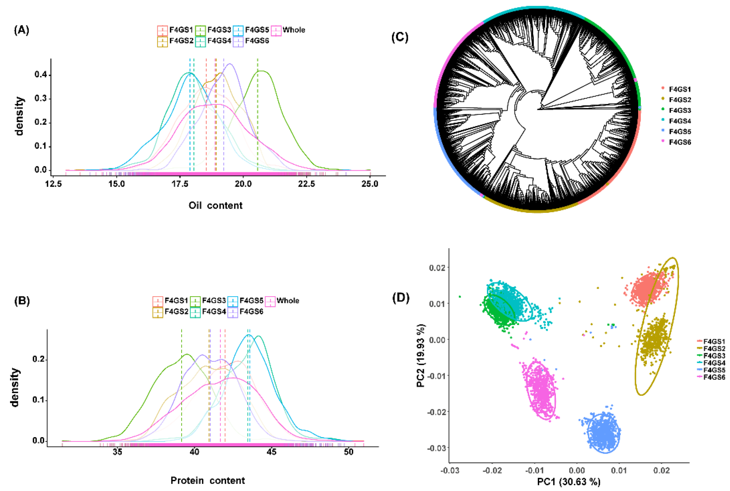
Figure 2.
Position distribution among soybean genome of 9,942 SNP markers from customizing panel(A); Distribution of quantitative trait nucleotides (QTNs) of the two traits viz., OC(B) and PC(C) identified via GWAS analysis across the soybean genome. The X-axis represents chromosomal coordinates, and that Y-axis represents significance level of QTNs. The color difference is to determine which chromosome QTNs belong to nereby.
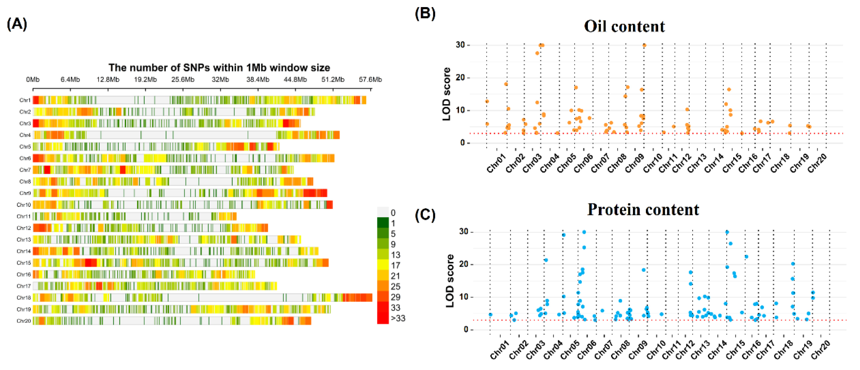
Figure 3.
GS prediction based on genome-wide SNPs marker and QTN using six different methods for OC (A) and PC (B). The height of the histogram represents the accuracy of the GS prediction, and the error bar represents the standard error of the prediction accuracy.
Figure 3.
GS prediction based on genome-wide SNPs marker and QTN using six different methods for OC (A) and PC (B). The height of the histogram represents the accuracy of the GS prediction, and the error bar represents the standard error of the prediction accuracy.
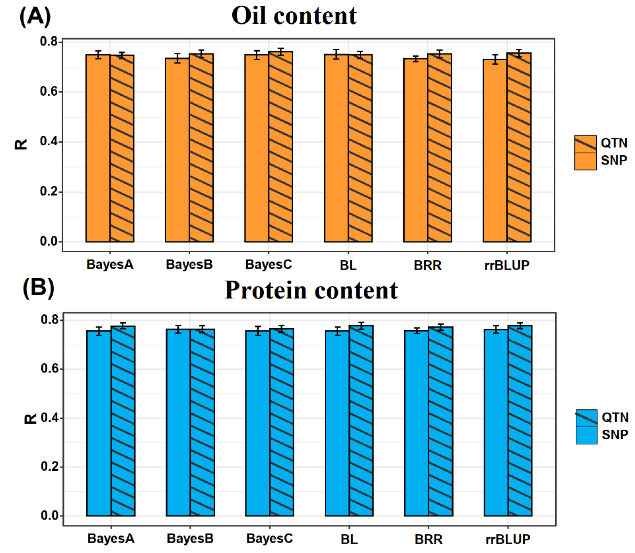
Figure 4.
Prediction accuracy of OC(A) and PC(B) with different training population size (Account for 10-90% of the whole population) comparison of prediction accuracy of genomic selection of oil content and protein content (using trait-specific QTNs, all QTNs and all SNPs. The height of the histogram represents the accuracy of the GS prediction, and the error bar represents the standard error of the prediction accuracy. The comparison among groups in the figure was performed using t-test, **** represented that P value < 0.0001, *** represented that P value < 0.001, * represented that P < 0.05, and ns represented that the difference was not significant.
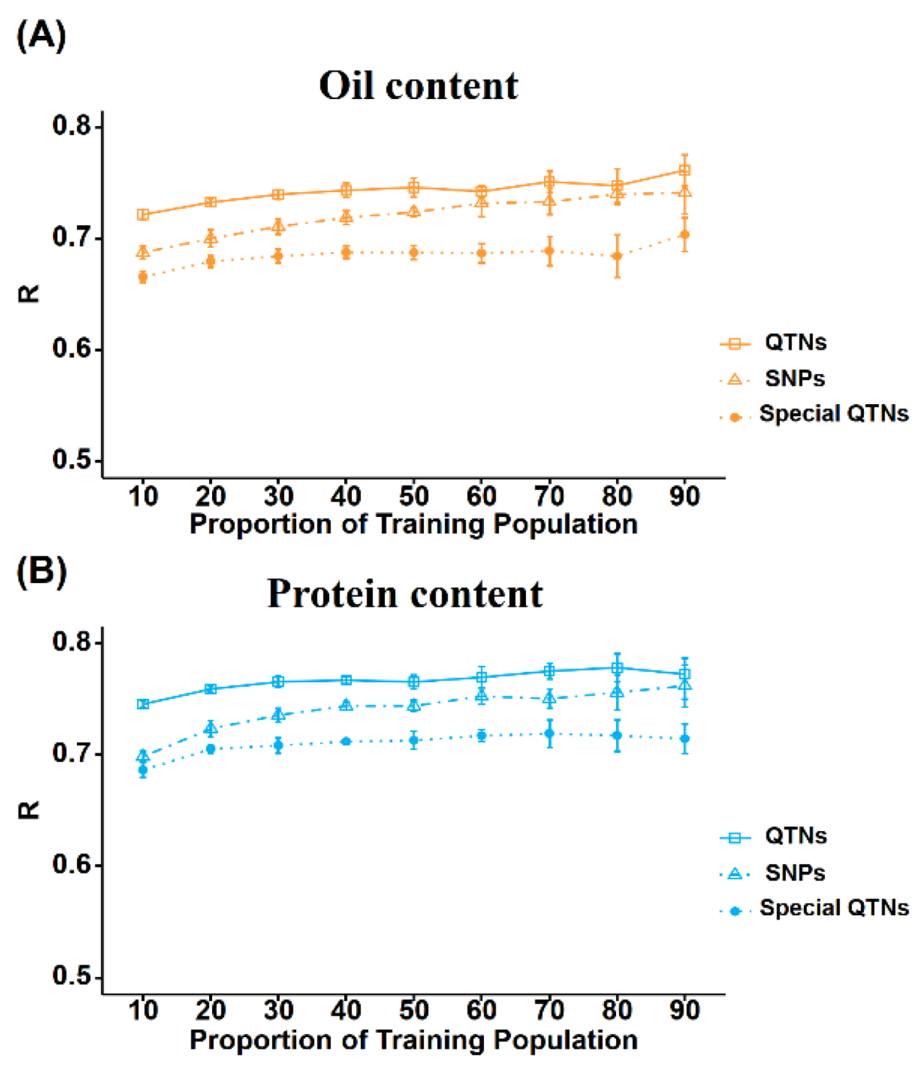
Figure 5.
Effect of subgroups screening using GS model with different QTNs set. Figure A and B show that true OC and PC distributions for the subgroups of the top20% individuals selected based on genomics selection using the two OC QTNs sets, respectively. Figure C and D show that true PC and OC distributions for the subgroups of the top20% individuals selected based on the genomics selection using the two PC QTNs sets, respectively. The comparison among groups in the figure was performed using t-test, **** represented that P value < 0.0001, *** represented that P value < 0.001, * represented that P < 0.05, and ns represented that the difference was not significant.
Disclaimer/Publisher’s Note: The statements, opinions and data contained in all publications are solely those of the individual author(s) and contributor(s) and not of MDPI and/or the editor(s). MDPI and/or the editor(s) disclaim responsibility for any injury to people or property resulting from any ideas, methods, instructions or products referred to in the content. |
© 2025 by the authors. Licensee MDPI, Basel, Switzerland. This article is an open access article distributed under the terms and conditions of the Creative Commons Attribution (CC BY) license (http://creativecommons.org/licenses/by/4.0/).
Copyright: This open access article is published under a Creative Commons CC BY 4.0 license, which permit the free download, distribution, and reuse, provided that the author and preprint are cited in any reuse.


