
Submitted:
15 September 2025
Posted:
16 September 2025
You are already at the latest version
Abstract
A long-standing challenge for the structural health monitoring (SHM) community is the masking effect of environmental variability, typically addressed by orthogonal projection (OP)-based data normalization to isolate the influence of environmental variability and enable structural anomaly detection. However, conventional OP techniques, such as principal component analysis, rely on clean and complete data, and their performance degrades in the presence of outliers or missing entries. To overcome this limitation, this paper proposes an integrated approach that combines OP with noisy low-rank matrix completion (NLRMC). The main advantage of NLRMC model is its ability to simultaneously perform low-rank and sparse decomposition with matrix completion, thereby recovering corrupted datasets and enabling robust anomaly detection. By incorporating novelty-indicator extraction, a fully online, unsupervised anomaly-detection procedure is established. Validation on a vibration-based SHM dataset from the KW51 railway bridge confirms that the NLRMC-OP approach achieves reliable detection of operational state changes before and after retrofitting, even under both data corruption and missing scenarios. This study advances the usability of SHM data and facilitates efficient decision-making, while also highlighting the broader significance of leveraging the low-rank data structure in AI-enabled operation and maintenance of civil infrastructure.
Keywords:
structural health monitoring
; anomaly detection
; orthogonal projection
; noisy low-rank matrix completion
; low-rank data structure
1. Introduction
In the wake of unprecedented large-scale infrastructure building, the ensuing long-term operation phase is marked by an increasing prevalence of deterioration mechanisms, including structural aging, material degradation, and damage initiation and propagation. These deterioration processes compromise the safety and functionality of infrastructure systems, while the associated demands for inspection, repair, and retrofitting continue to escalate. Structural health monitoring (SHM), a critical field bridging engineering, data science, and materials re-search, enables the detection of potential anomalous behaviors, complementing visual inspections and supporting condition assessment and long-term operation and maintenance [1,2,3]. Recent advances in sensing technologies, including smartphones [4], computer vision [5], non-contact testing [6], and unmanned aerial vehicles [7], together with developments in communication networks such as the Internet of Things [8], cloud computing [9] and even block-chain [10], have expanded the capability and accessibility of SHM to acquire richer structural responses and extract features from raw measurements. Naturally, harnessing these data and features while interpreting them for structural anomaly detection has become increasingly critical.
SHM data interpretation faces substantial challenges from environmental variability, including time-varying temperature, humidity, wind, and uneven solar exposure, which can obscure or mimic genuine signatures of structural deterioration or anomalies [11,12,13]. Among these factors, temperature is one of the most pervasive and problematic: variations in thermal conditions can alter elastic moduli and sensor responses, generating signals that are difficult to distinguish from those associated with actual deterioration [14]. One conventional solution is direct compensation, which corrects new measurements by constructing regression models that relate recorded environmental factors, e.g., temperature, to structural responses [15,16]. While conceptually straightforward, such methods face inherent limitations: the complexity of environmental influences often defies complete measurement, and as structural changes, damage progression, and aging effects occur, the originally fitted regression models may become obsolete, thereby diminishing their effectiveness.
To overcome these limitations, unsupervised data normalization offers an efficient alternative, primarily relying on data-driven learning. These approaches streamline implementation and circumvent the challenges posed by long-term, intricate environmental observations [12]. In practice, unsupervised machine learning (ML) models, applied either individually or in combi-nation, often adopt a residual strategy that exploits redundancy arising from spatiotemporal correlations in the measured dataset, rendering it intrinsically low-rank. This involves con-structing a low-rank/dimensional subspace dominated by environmental variability and computing residuals between the raw data and its projection onto this subspace, thereby isolating the influence of environmental variability and enabling anomaly detection. The implementation of this strategy contingent upon constructing the low-rank/dimensional subspace via orthogonal projection (OP), employing classical matrix decomposition techniques [17,18,19] such as principal component analysis, eigenvalue decomposition, factor analysis, and independent com-ponent analysis, as well as through cointegration analysis [20] and autoencoder neural net-works [21]. Other unsupervised approaches include clustering [22] and transfer learning [23], in which a baseline pattern is first learned and anomalies are subsequently detected via shifts in feature distributions.
Nevertheless, the quality of the acquired data is not always sufficient for the effective implementation of the aforementioned unsupervised ML algorithms. Corrupted or missing data can severely compromise data normalization processes such as principal component analysis, thereby disrupting the structural anomaly detection pipeline [12,24,25]. From a data cleansing perspective, the low-rank structure inherent in the measured dataset can be fully leveraged. Low-rank matrix recovery approaches constitute a family of computational approaches, including robust principal component analysis (RPCA), matrix completion, non-negative matrix factorization and low-rank representation. Among them, RPCA model, which decomposes the raw data matrix into the sum of a low-rank matrix and a sparse noise matrix, has proven particularly effective in handling grossly corrupted entries [26,27]. Yang and Nagarajaiah [28,29] introduced the low-rank and sparse matrix decomposition methods for dynamic-imaging-based inspection of local structural damage, and later extended its application to two-dimensional strain fields with dense sensor layouts, successfully identifying sparse damage patterns. They further put forward the concept that multi-channel noisy structural vibration responses possess an intrinsic low-rank data structure, which can be exploited for system identification and anomaly detection [30,31]. Song et al. [32] employed RPCA to remove sparse noise from distributed strain data obtained via fiber optic sensing, thereby enabling more accurate detection of structural microcracks.
Over the past decades, vibration-based SHM has emerged as a primary means of evaluating global structural condition. Within this framework, natural frequency has been the most widely adopted feature, owing to its direct link to intrinsic structural properties and its relative ease of extraction through operational modal analysis. However, as highlighted in the preceding discussion, natural frequency is profoundly sensitive to environmental variability, making anomaly detection highly susceptible to confounding influences. Unsupervised ML models, particularly those grounded in data normalization process, such as OP, provide effective tools to mitigate such effects, yet their successful deployment hinges on the reliability of the underlying data [33]. In this context, corrupted or missing entries in datasets present a critical bottle-neck, and addressing this issue has become essential to ensure the robustness of the anomaly detection pipeline. Maes et al. [34] demonstrated that the low-rank data structure in sets can be harnessed to support principal component analysis, thereby enabling robust anomaly detection even when the data is corrupted. Xu et al. [35] employed low-rank matrix approximation to pre-process imperfect frequency dataset prior to cointegration analysis, enhancing robustness in the presence of noisy or missing data. Notably, multi-order natural frequencies are prone to substantial missing entries as a consequence of the low success rate of in-situ modal identification. When frequency datasets with such gaps are used for structural anomaly detection, the unavoidable removal of samples significantly undermines the capacity to assess structural condition in a timely and reliable manner.
This paper proposes exploiting the low-rank data structure inherent to robustly tackle structural anomaly detection under environmental variability. While OP-based residual strategies can isolate the influence of environmental variability, the presence of corrupted or missing data often hinders the reliable implementation of such data normalization process. To address this issue, a noisy low-rank matrix completion (NLRMC) model is introduced as a preprocessing step to recover the corrupted and missing data. The NLRMC model is expected to exert its advantage by simultaneously performing low-rank and sparse decomposition together with matrix completion, enabling the elimination of potential corruptions in the raw data matrix while imputing the missing entries, and ultimately ensuring the smooth execution of unsupervised pipeline. Besides, a moving window-based online anomaly-detection procedure is established following the integration of the NLRMC-OP approach with feature fusion and classification steps under unsupervised ML framework, from which a novelty indicator is extracted to assess the structural condition.
The structure of this paper is as follows. Section 2 presents the methodology underlying the proposed online robust anomaly-detection procedure. This section emphasizes the theoretical exposition of the OP-based residual strategy and its limitations, as well as the introduction of the NLRMC model to compensate for the shortcomings of RPCA. It further includes theories of feature-fusion and classification steps that are essential for novelty-indicator extraction. The datasets and their subsets, to which the above methodology is applied are described in Section 3. In Section 4, the effectiveness and robustness of the proposed approach are substantiated under two subsets with different levels of data completeness.
2. Methods
2.1. OP-Based Residual Strategy for Anomaly Detection
In the context of long-term SHM activities, the measured structural response data are inevitably influenced by various environmental factors, which may obscure the presence of structural anomaly. In an unsupervised setting, orthogonal projection (OP)-based residual strategy is capable of decoupling environmental variability from structural anomaly-related components in the measured responses [17,18,19]. The core principle underlying the OP-based models lies in the fact that multi-channel sensing data or multi-order modal features inherently exhibit a low-rank/dimensional structure, which can be explicitly modeled [12,33,34].
Herein, the term low-rank is primarily used to describe the mathematical property of the data matrix, reflecting its approximate rank deficiency due to the strong correlations among variables, whereas low-dimensional is adopted when interpreting the OP of the raw data matrix onto a low-rank/dimensional subspace or hyperplane, where deviations from this subspace or hyperplane can be regarded as indicative of structural anomalies induced by structural changes or damage progression. Unless otherwise stated, the two terms are closely related and the term low-rank is used more frequently throughout this paper.
At time , the incoming measuring samples are organized into a column vector , with corresponding to the total number of sensing channels or identified modal orders. We define a baseline low-rank subspace that captures the normal-state variability of structural response data related to time-varying environmental factors. This subspace is learned from baseline samples assumed to be free from structural changes or damage progression. Given a new sample , the OP loss of onto the low-rank subspace of , denoted residual vector , is computed as:
where is the OP operator onto . The residual vector quantifies the orthogonal component of that cannot be explained by the low-rank subspace , and is thus hypothesized to reflect structural anomalies. Moreover, the norm of serves as an anomaly score, where a larger magnitude indicates a higher likelihood of deviation.
Mathematically, under the assumption that each dimension of the data matrix follows an independent Gaussian distribution, the explicit model can be constructed through eigenvalue decomposition. If denotes the data matrix with samples of , the eigenvectors of the covariance matrix of can serve as the basis vectors for the OP model. The covariance of is equivalent to , where is the sample mean of with each row centered. Computationally, eigenvalue decomposition is then applied to obtain:
where is an orthonormal matrix comprising with singular vectors or called eigenvectors; represents a zero-truncated eigenvalue value matrix with diagonal elements, each corresponding to an eigenvalue.
From the perspective of cumulative variance contribution, the eigenvalues are sorted in descending order, and the first eigenvectors form the matrix (with ), which are primarily influenced by a limited number of time-varying environmental factors and account for the largest proportion of the projection energy. The basic vectors in thus span a low-rank subspace. The residual matrix , i.e., the OP loss of onto the low-rank subspace, is estimated as:
By comparing Eq. (1) and Eq. (3), it can be observed that the OP operator can be given by . Based on the operator learned under the normal state, and Eq. (1), anomaly detection, also referred to as novelty detection, can be performed.
During long-term SHM implementation, corrupted entries may arise in the dataset owing to measurement irregularities under harsh in-service environments. In particular, extreme low-temperature conditions can generate outliers in natural frequencies [34,35], thereby limiting the applicability and performance of Gaussian noise-based OP models, which are inherently non-robust to such corruptions. As illustrated in Figure 1, the presence of corrupted data points (black crosses) can substantially bias the estimated subspace obtained through OP (blue dashed line). Instead of aligning with the underlying true low-rank subspace defined by clean observations (red crosses along the gray line), the projection is distorted toward corrupted data, thereby undermining the reliability of the data normalization process and hindering accurate anomaly detection.
2.2. NLRMC
To overcome the limitations of OP model, RPCA [26,27] aims to recover the intrinsic low-rank structure of the measured data matrix by decomposing it into two additive components: a low-rank matrix that captures the dominant structural responses, and a sparse matrix that accounts for corrupted measurements. The optimization problem is classically formulated as:
where the rank function enforces the low-dimensional structure of , the -norm promotes sparsity in , and controls the trade-off between enforcing the low-rank structure and suppressing sparse corruption.
Since directly solving this nonconvex problem is NP-hard, convex relaxations are typically adopted, enabling the separation of informative low-rank subspaces from sparse outliers in a computationally tractable manner. The rank function is replaced with the nuclear norm , which is the sum of singular values of , and the -norm is replaced with the -norm to promote sparsity in . The relaxed problem can thus be written as:
It is worth noting that the application of the RPCA-assisted OP model differs substantially from its widespread use in computer vision. In visual detection, RPCA is often employed to extract the low-rank background component of images and capture both the onset and progression of local damage from the sparse component. This distinction underscores RPCA’s role not merely as a background-foreground separator but as a data cleansing mechanism tailored for long-term SHM without relying on the assumption of small Gaussian noise.
By isolating outliers into the sparse matrix , RPCA effectively eliminates their influence on the estimation of the low-rank subspace . Though offering a powerful framework to recover the low-rank structure from corrupted measurements, RPCA’ s basic formulation assumes that all entries of the data matrix are fully observed. Incomplete observations such as the presence of missing data cannot be adequately resolved. In fact, when RPCA was first proposed, Candès et al. [27] had already considered the possibility of missing entries, which in turn stimulated the development of matrix completion approaches. The standard RPCA formulation alone cannot accommodate data incompleteness, whereas matrix completion methods, although effective for imputing missing values, are inherently vulnerable to sparse outlies.
To this end, this study introduces the NLRMC model [36,37], which combines the complementary strengths of RPCA and matrix completion. The primary goal of the NLRMC model is to recover the raw data matrix by performing a synergic low-rank sparse decomposition and matrix completion. This mitigates the adverse effects of gross sparse noise while imputing missing entries simultaneously. Formally, given a data matrix , let denote the set of observed entries, and also define the projection operator such that:
The recovery problem is then formulated as
where the projection constraint ensures consistency with available observations.
The NLRMC model provides a robust data cleansing mechanism that yields a nearly low-rank representation of the raw data matrix. This preprocessing step not only suppresses spurious outliers but also imputes missing entries, thereby enhancing the robustness of subsequent ML framework and strengthening traditional data normalization procedures. It is worth noting that when the data matrix contains no missing entries, the NLRMC model naturally degenerates to the RPCA formulation.
In this study, we adopt the solver proposed by Lu et al. [38], which addresses the NLRMC problem through an Alternating Direction Method of Multipliers (ADMM) framework enhanced by Majorization Minimization. The optimization variables are updated in two super-blocks, consisting of the pair (,) and an auxiliary variable. In this formulation, is computed via proximal nuclear norm minimization, whereas is obtained through soft-thresholding or related proximal operators depending on the chosen loss function. This strategy not only ensures stable convergence but also provides the flexibility to accommodate different noise models. Compared with conventional nuclear norm-based approaches, the nonconvex formulation and Majorization Minimization-augmented ADMM solver yield tighter approximations to the true matrix rank and significantly accelerate convergence in practice.
2.3. Novelty Indicator Extraction Within Unsupervised ML Framework
The NLRMC model provides a robust preprocessing step to recover the low-rank data matrix, upon which the OP-based data normalization process can calculate residual vectors as anomaly scores, referred as the NLRMC-OP approach in this paper. Besides, the discriminative capability of these scores alone remains limited for reliably separating normal and abnormal states. Therefore, subsequent efforts focus on translating these residuals into actionable novelty detection outcomes within an unsupervised ML framework. Given the unknown evolution trends of multi-channel sensing data or multi-order modal features under structural changes, feature-level fusion is required to derive a unified indicator that consolidates the available information. Once this fused indicator is obtained, control chart techniques are applied to extract the final indicators, enabling the classification of structural patterns into normal or abnormal states.
Mahalanobis distance (MD) is computed on the OP-based residual vectors to fuse multi-channel sensing data or multi-order modal features into a single statistic that captures the unified evolutionary trend. Let and be the mean and covariance estimated from the baseline residuals; for a residual vector , the squared MD is
Using baseline-only and aligns the indicator with the normal-state distribution and provides scale and correlation normalization, which improves discriminability for coordinated shifts while attenuating uninformative variance. The resulting MD sequence serves as the fused indicator that feeds the subsequent control chart step.
Among the control charts used in SHM, including the X-bar, Shewhart-T, and Hotelling T² charts [39], this study adopts the exponentially weighted moving average (EWMA) chart. EWMA remains reliable when the fused indicator departs from normality and, by combining current observations with historical information through exponential weighting, is particularly sensitive to small, sustained shifts that enable early detection of subtle anomalies. Let denote the fused indicator (MD) corresponding to the sample at time . The EWMA statistic is updated as:
where is a constant that determines the proportion of information contributed by the current sample relative to preceding samples; is set to the mean value of the baseline MDs; is the controlled variable to be detected, serving as the novelty indicator (NI) in this study for evaluating the structural condition.
With the control variable defined, an abnormal trend is identified when the statistic exceeds predetermined bounds. For the EWMA chart, these bounds are specified by the upper control limit (UCL) and lower control limit (LCL), which are computed as
where is the standard deviation of the baseline MDs and is a tunable parameter that defines the width of control limit in the EWMA control chart.
2.4. Implementation of Online Unsupervised Procedure
The moving-window strategy, using short data matrices at fixed intervals, refers to the implementation of online anomaly-detection procedure. The motivation arises from the fact that a limited number of sensing channels or modal features ( dimensions), combined with the large volume of observations ( samples) accumulated in long-term SHM activities, yields a slender data matrix of size (), which imposes computational burdens. The window size should be sufficiently larger than the period of dominant environmental variations, yet smaller than the total number of samples in the training dataset [40].
The proposed online robust anomaly-detection procedure based on moving windows is illustrated in Figure 2. In this framework, the two key steps are the aforementioned NLRMC and OP, which act as data cleansing and normalization operations within each moving window. At each iteration , a window of length is constructed starting from the current sample and encompassing the subsequent samples; once the analysis within the current window is completed, the window is shifted forward to update the computation. The entire procedure consists of two phases: (i) training phase, during which baseline features are extracted and control limits are established, and (ii) monitoring phase, in which new samples are sequentially processed to enable online anomaly detection.
Training phase:After initializing the moving-window size and the parameters of the control chart, the data matrix constructed from the first window is adopted as the baseline for unsupervised training. NLRMC is then applied to perform data cleansing, which simultaneously completes missing entries and isolates corrupted components, thereby producing a baseline low-rank matrix. Subsequently, OP-based residual strategy is employed to derive the eigenvector matrix and compute the corresponding residual vectors. At the end of the training phase, MD-based feature fusion is performed based on these residual vectors, and the EWMA-based control limits (CLs) are established for subsequent monitoring.
Monitoring phase:The moving-window process is implemented in real time, and within each updated window the unsupervised learning procedure described above is executed. The data matrix is updated by appending one column of the newly acquired feature data and removing the earliest column, as depicted in Figure 2. For each updated data matrix, NLRMC and OP are applied to compute the residual vectors, followed by feature fusion and control charting to obtain the NI. Anomaly detection is then carried out by comparing this indicator against the CLs obtained in the training phase. The structure is considered to remain in its normal state during that window. Conversely, a NI value exceeding the UCL or LCL signals the occurrence of a structural anomaly. From a subspace perspective, when no structural changes or damage progression are present, new samples are expected to lie within the hyperplane spanned by the low-rank subspace of the normal state. In contrast, abrupt changes or progressive damage drive the features away from this hyperplane, producing substantially larger residuals that indicate an abnormal state.
3. Application to the KW51 Bridge
Because real-world cases of structural anomaly monitoring are rare, validating structural anomaly detection approaches often relies on artificially induced scenarios, such as generating frequency shifts from numerical models. In this study, however, we employ the publicly available dataset of the KW51 railway bridge released by Maes and Lombaert [34], which has become a benchmark in the SHM community for its ability to capture genuine structural changes across three operational states -before, during, and after retrofitting. The KW51 bridge is a 115 m long, 12.4 m wide steel tied-arch structure with a dual-track deck suspended by inclined hangers, located on the L36N railway line between Leuven and Brussels and serving various passenger trains since 2003. Between May and September 2019, the bridge underwent retrofitting to strengthen bolted connections between the braces, the deck, and the arch; scaffolding installed during this period temporarily altered its mass and stiffness. After reinforcement with welded steel plates, the bridge returned to service. This distinctive sequence of operational states can therefore be used to evaluate the effectiveness and robustness of the proposed procedure for detecting anomalies in real-world structural conditions.
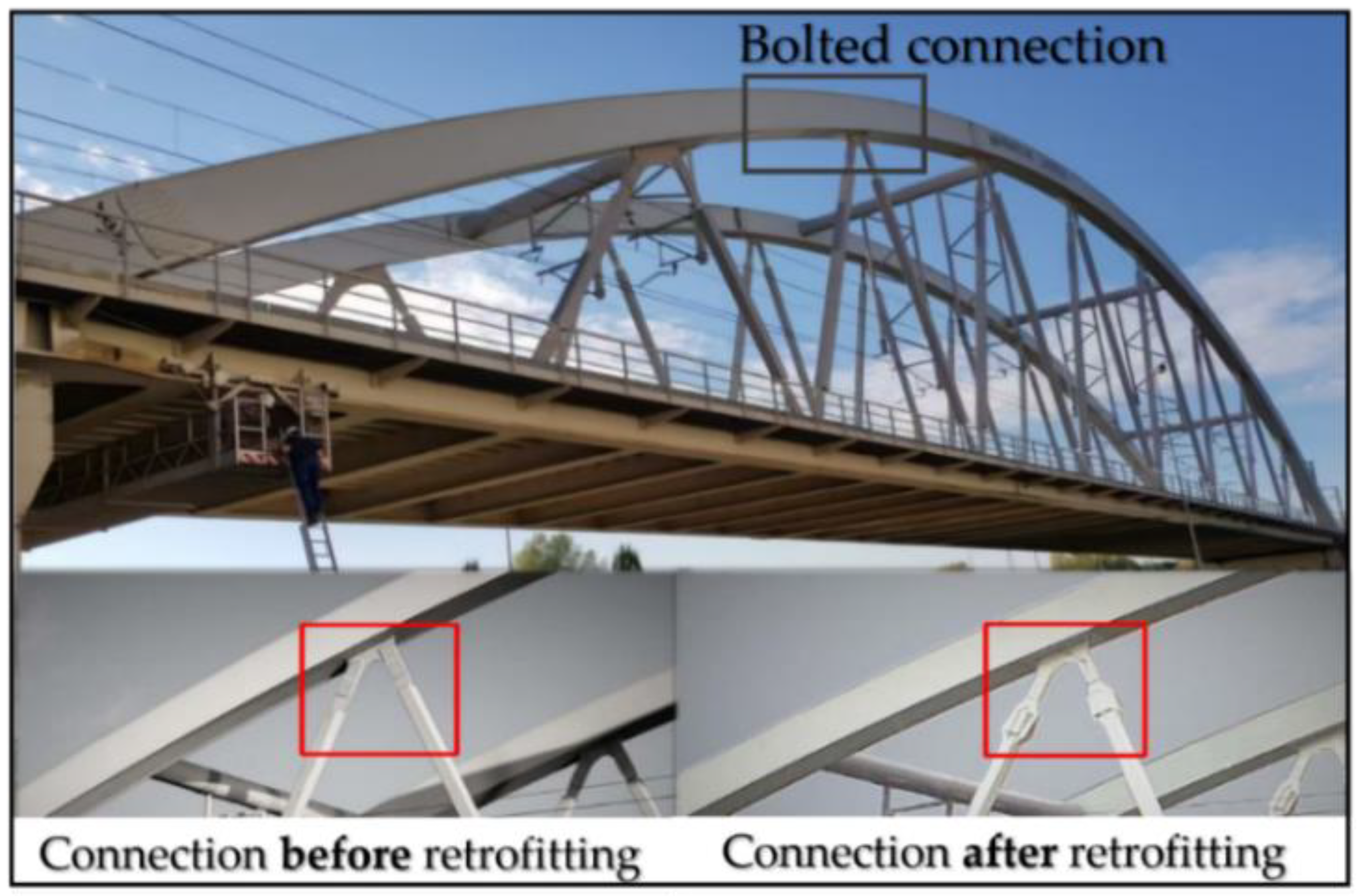
Figure 3.
The KW51 bridge and its structural changes on its connections.
The monitoring campaign of the KW51 bridge spanned three operational states: a 7.5-month period before retrofitting (2 October 2018 – 15 May 2019), the retrofitting period (16 May – 27 September 2019) and a 3.5-month period after retrofitting (28 September 20 15 January 2020). During this time, the sensor network was progressively enhanced, yielding a dataset comprising acceleration, strain, displacement, temperature and humidity measurements. Structural vibration responses from train-induced and ambient sources were captured by 12 accelerometers installed on the deck and arches. Operational modal analysis was conducted on an hourly basis based on ambient vibration responses to track the evolving dynamic characteristics of the KW51 bridge.
A total of 14 modal frequencies were identified throughout the monitoring campaign and categorized into two groups [34]. The first is an increasing group (modes 6-8 and 10-14), whose frequencies rose after retrofitting owing to the stiffening of the connections between the diagonals, the deck, and the arches. The second is a decreasing group (modes 1-5 and 9), which exhibited reductions as a result of the added mass from the retrofitted steel boxes near the arches. Previous analyses [23] examined these features in their original spaces and histograms, revealing a pronounced masking effect in which environmental variability, particularly temperature, dominated the frequency distributions. Only six natural frequencies were selected to verify the proposed approach, as shown in Figure 4, with particular attention to the NLRMC-OP approach. The six modes include three from the increasing group (modes 6, 10, and 13) and three from the decreasing group (modes 3, 5, and 9). Furthermore, to comprehensively assess the approach’s performance under varying levels of data completeness, two subsets were defined. Dataset 1 excludes all frequency vectors containing missing entries, yielding 2,524 and 677 samples corresponding to the operational states before and after retrofitting, respectively. Dataset 2 removes only those vectors with all entries missing, resulting in 4,090 and 2,555 samples before and after retrofitting, respectively. Together, these datasets provide a rigorous basis for evaluating the proposed approach in handling corrupted and missing data under realistic SHM applications.
For methodological comparison, the proposed online anomaly detection procedure was applied without the NLRMC-OP steps, that is, by directly performing feature fusion and classification on the multi-order raw frequency data, i.e., Equations (8)-(11), yielding a pseudo novelty-detection result. As shown in Figure 5, the substantial structural changes of the KW51 bridge before and after retrofitting enabled a relatively straightforward distinction between the two operational states. Nevertheless, the reliability of the NIs obtained under this setting remains highly questionable. When the initial control-limit width was set to 5, a large number of outliers appeared in the indicators before-retrofitting (normal) state, which typically arose from material nonlinearities near 0 °C caused by freezing effects [34], ultimately leading to false positives. Even after adjusting the control-limit width to 25, structural anomalies after retrofitting were still misclassified as normal, as evidenced by the data points after the blue dashed line in Figure 5, reflecting more severe false negatives. These deficiencies highlight the lack of robustness in anomaly detection using statistical models alone and underscore the necessity of incorporating data normalization and cleansing steps into the proposed unsupervised pipeline to avoid misleading decision-making.
Furthermore, Dataset 1, which excludes all frequency vectors containing missing entries, substantially reduced the utilization rate of the raw frequency data. Referring to Table 1, two quality indexes are reported for the six selected modes: the success rate (SR), which represents the modal identification success rate of each modal frequency, and the utilization rate (UR), which denotes the proportion of measurement samples that remain usable in the multi-order frequency dataset after removing missing entries. Mode 10 in Table 1 exhibited a relatively low success rate of modal identification, resulting in numerous gaps in the frequency dataset. The removing gaps of samples in Dataset 1 caused the URs of the raw frequency data for the other modes to fall to less than half. More importantly, the first sample in Dataset 1 after retrofitting (i.e., the 2525th sample) corresponds to a timestamp of 18:00 on 28 September 2019, even though the actual retrofit having been completed on 27 September 2019. In reality, monitoring of such structural changes due to after retrofitting started at midnight on 28 September, so the gap-removal operation in Dataset 1 deleted all samples between 00:00 and 18:00. This omission prevented the timely detection of structural changes that occurred in the bridge, thereby leading to false negatives. Hence, Dataset 2, with 100% utilization yet containing substantial missing entries, is indispensable for demonstrating the effectiveness of the proposed online robust anomaly-detection procedure.
4. Results
4.1. Structural Anomaly Detection with Complete Dataset (Dataset 1)
Preliminary verification was conducted on Dataset 1. The gap-removal operation excluded a large number of samples, thereby restricting the discussion to the condition of a complete dataset. The parameters for the training phase were preset as follows: the regularization parameter in Equation (7) was assigned the value [34], consistent with that used in the RPCA model; the moving-window size was set to 70% of the known period before retrofitting within the unsupervised ML framework; and the control-limit width was fixed at 5. The complete pipeline of the proposed online robust anomaly-detection procedure was then executed, with the OP-based residuals of all modes plotted in Figure 6. As can be seen, even before MD-based feature fusion, the residuals could be clearly distinguished, with few false positives observed.
The novelty indicators corresponding to Dataset 1 are presented in Figure 7. Compared with the results in Figure 5, the combined use of the NLRMC and OP models effectively mitigated the adverse impacts of the freezing effect. As further illustrated in the subgraph, the sparse outliers in the raw frequency dataset (represented by the blue points below 0°C in Figure 4) did not lead to false positives in the final NI results. The proposed approach thus improves the robustness of structural anomaly detection in the presence of data corruption induced by complex environmental conditions. It should be noted that, because Dataset 1 contained no missing entries, the role of the NLRMC model as a preprocessing step could not be demonstrated.
4.2. Structural Anomaly Detection with Incomplete Dataset (Dataset 2)
In Dataset 1, where no missing entries were present, the first structural anomaly corresponding to the 2,525th sample, was successfully identified, as shown in the subgraph of Figure 7. However, the associated timestamp (18:00 on 28 September 2019) indicates that this detection occurred 18 hours after the actual start of structural changes (00:00 on 28 September 2019), resulting in a considerable delay. For structural anomalies induced by structural changes or damage progression, such a delay would be unacceptable. This shortcoming highlights that directly removing all frequency vectors containing missing entries is not a viable strategy. To further substantiate the role of NLRMC model in the proposed anomaly-detection procedure, Dataset 2 was therefore adopted. In Dataset 2, samples 1-4,090 and 4,091-6,645 correspond to the operational states before and after retrofitting, respectively. Unlike Dataset 1, Dataset 2 retains all frequency vectors that contain at least one successfully identified entry in raw frequency dataset. The URs of the selected modal frequencies in Dataset 2 reached 100%.
Mode 10, which shows a particularly low success rate of modal identification, was selected to specifically demonstrate the role of the NLRMC model as a preprocessing step, as illustrated in Figure 8. The measured frequency series, represented by the black scatters, contained numerous gaps, whereas the incomplete data were imputed as the red plots. It should be noted that this imputation was achieved through recovering the low-rank matrix in Equation (7). The purpose of applying the low-rank matrix completion technique here is not to obtain an exact imputation of the missing values, but rather to enable to carry out the subsequent OP-based residual calculation, which then serves to indicate whether the operational state is normal or abnormal.
The problem of incomplete data is a critical issue in long-term SHM, commonly arising from sensor malfunction, transmission errors, device maintenance, or structural retrofitting. Left untreated, missing entries can cause algorithmic failure, biased inference, and misleading decision-making. In Dataset 2, where incomplete frequency vectors were retained, the 4,091st sample - corresponding to 00:00 on 28 September 2019 - was identified without delay, free from both false positives and false negatives. Results illustrated in Figure 9 and Figure 10 confirms that the proposed approach can achieve timely and reliable anomaly detection, even under incomplete data conditions. Unlike the RPCA model, which cannot operate when the data matrix is only partially observed, the integration of NLRMC into the anomaly detection procedure enables the simultaneous recovery of the underlying low-rank structure, isolation of corrupted components, and completion of missing entries. By fully exploiting the intrinsic low-rank data structure, the inclusion of NLRMC as a preprocessing step enhances data utilization, ensures the operability of OP-based residual strategy under severely data missing conditions, and ultimately delivers robust anomaly-detection results that are both timely and reliable.
5. Conclusions
This paper addresses the challenge of robust anomaly detection in the SHM community. Although conventional OP techniques, such as principal component analysis, have been shown to be effective in isolating environmental effects, its performance can be impaired by corrupted or missing data. Motivated by the intrinsic low-rank nature of the measured dataset, we introduced the NLRMC model as a preprocessing step for OP-based data normalization. By jointly performing low-rank and sparse decomposition and matrix completion, the NLRMC model mitigates the adverse influence of sparse outliers while simultaneously imputing missing entries. Building upon this foundation, the integration of the NLRMC-OP approach with MD-based feature fusion and EWMA control chart under unsupervised ML framework forms a fully unsupervised online anomaly-detection procedure. The proposed approach was substantiated using the KW51 bridge, whose distinctive sequence of operational states provides a rigorous basis for assessing its effectiveness and robustness under realistic SHM conditions. The main conclusions of this study are as follows:
Firstly, the two operational states before and after retrofitting could still be separated by directly applying an online procedure using the raw frequency dataset, even without incorporating the NLRMC-OP approach. However, the freezing effect near 0°C generated sparse outliers, leading to false positives, while structural anomalies due to retrofitting were misclassified as normal when the control-limit width was enlarged, resulting in false negatives.
Secondly, when the proposed NLRMC-OP approach was applied to Dataset 1, the sparse outliers induced by the freezing effect were effectively tackled. As a result, the adverse influence of environmental variability was suppressed, ensuring that these outliers no longer produced false positives or negatives. The proposed approach thus improves the robustness of structural anomaly detection in the presence of data corruption induced by complex environmental conditions.
Finally, unlike the gap-removal operation applied in Dataset 1, Dataset 2 retained all frequency vectors with at least one identified natural frequency and was therefore employed to evaluate the approach’s performance on a dataset that, although not fully complete, preserved all the available samples. The results confirm that integrating NLRMC with OP enables the detection of the first anomaly immediately after retrofitting, at 00:00 on 28 September 2019, without delay or misclassification. This demonstrates that the proposed approach improves data utilization rate and delivers robust, timely anomaly detection - a capability that cannot be simultaneously achieved using the RPCA model.
The synergy of NLRMC transforms the vulnerability of OP operators to outliers and missing data into a robust component of an unsupervised ML framework for structural anomaly detection. Both OP and NLRMC techniques are rooted in the low-rank data structure, or more generally, low-dimensional modeling. Amid the wave of AI-enabled civil infrastructure, approaches that exploit the inherent low-rank data structure could offer a robust pathway to overcome masking effects, thereby enhancing SHM data usability and decision reliability.
Author Contributions
Conceptualization, Peng Ren and Le Zhou; methodology, Peng Ren; software, Peng Ren; validation, Heng Zhang, Peng Ren and Peng Niu; resources, Peng Ren; data curation, Wei Li and Xiaochu Wang; writing - original draft preparation, Peng Ren; writing - review and editing, Peng Ren; funding acquisition, Le Zhou. All authors have read and agreed to the published version of the manuscript.”
Funding
This research was funded by National Natural Science Foundation of China, with grant number 52478191.
Acknowledgments
The datasets for the KW51 bridge are available at Maes and Lombaert [34], https://doi.org/10.5281/zenodo.3745914. We gratefully acknowledge their generous contribution in making these data publicly available to the scientific community.
Conflicts of Interest
The authors declare no conflicts of interest.
Abbreviations
The following abbreviations are used in this manuscript:
| SHM | Structural health monitoring |
| ML | Machine learning |
| OP | Orthogonal projection |
| NLRMC | Noisy Low-rank Matrix Completion |
| RPCA | Robust Principle Component Analysis |
| ADMM | Alternating Direction Method of Multipliers |
| MD | Mahalanobis distance |
| EWMA | Exponentially weighted moving average |
| CL | Control limit |
References
- Doebling, S.W.; Farrar, C.R.; Prime, M.B.; et al. Damage Identification and Health Monitoring of Structural and Mechanical Systems from Changes in their Vibration Characteristics: A Literature Review. Washington DC: Los Alamos National Lab, 1996, LA-13070-MS.
- Bao, Y.Q.; Li, H. Machine learning paradigm for structural health monitoring. Struct. Health Monit. 2020, 19, 1–20. [Google Scholar] [CrossRef]
- Sun, L.M.; Shang, Z.Q.; Xia, Y.; et al. Review of Bridge Structural Health Monitoring Aided by Big Data and Artificial Intelligence: From Condition Assessment to Damage Detection. Journal of Bridge Engineering 2020, 146, 04020073. [Google Scholar] [CrossRef]
- Sarmadi, H.; Entezami, A.; Yuen, K.-V.; Behkamal, B. Review on smartphone sensing technology for structural health monitoring. Measurement 2023, 223, 113716. [Google Scholar] [CrossRef]
- Feng, D.; Feng, M.Q. Computer vision for SHM of civil infrastructure: From dynamic response measurement to damage detection – A review. Eng Struct. 2018, 156, 105–17. [Google Scholar] [CrossRef]
- Brien, E.J.; Keenahan, J. Drive-by damage detection in bridges using the apparent profile. Struct Control Health Monit 2015, 22, 813–825. [Google Scholar]
- Bacco, M.; Barsocchi, P.; Cassara, P.; et al. Monitoring ancient buildings: real deployment of an IoT system enhanced by UAVs and virtual reality. IEEE Access 2020, 8, 50131–50148. [Google Scholar] [CrossRef]
- Al-Turjman, F.; Abujubbeh, M.; Malekloo, A. Deployment strategies for drones in the IoT Era: a survey. In Drones in IoT-enabled spaces; CRC Press/Taylor & Francis Group: Boca Raton, FL, 2019; pp. 7–42. [Google Scholar]
- Luo, L.; Feng, M.Q.; Wu, J.; et al. Autonomous pothole detection using deep region-based convolutional neural network with cloud computing. Smart Struct Syst 2019, 24, 745–757. [Google Scholar]
- Xu, J.; Liu, H.; Han, Q. Blockchain technology and smart contract for civil structural health monitoring system. Comput-Aided Civ Infrastruct Eng 2021, 12666. [Google Scholar] [CrossRef]
- Erazo, K.; Sen, D.; Nagarajaiah, S.; Sun, L.M. Vibration-based Structural Health Monitoring under changing environmental conditions using Kalman filtering. Mech. Syst. Signal Process. 2019, 117, 1–15. [Google Scholar] [CrossRef]
- Malekloo, A.; Ozer, E.; AlHamaydeh, M.; Girolami, M. Machine learning and structural health monitoring overview with emerging technology and high-dimensional data source highlights. Struct. Health Monit 2022, 21(4), 1906–1955. [Google Scholar] [CrossRef]
- Radulescu, V.M.; Radulescu, G.M.T.; Nas, S.M.; Radulescu, A.T.; Radulescu, C.M. Structural health monitoring of bridges under the influence of natural environmental factors and geomatic technologies: a literature review and bibliometric analysis. Buildings 2024, 14, 2811. [Google Scholar] [CrossRef]
- Fendzi, C.; Rébillat, M.; Mechbal, N.; Guskov, M.; Coffignal, G. A data-driven temperature compensation approach for structural health monitoring using lamb waves Struct. Health Monit. 2016, 15, 525–40. [Google Scholar] [CrossRef]
- Ding, Y.L.; Wang, G.-X.; Hong, Y.; Song, Y.-S.; Wu, L.-Y.; Yue, Q. Detection and Localization of Degraded Truss Members in a Steel Arch Bridge Based on Correlation between Strain and Temperature. J. Perform. Constr. Facil. 2017, 31, 04017082. [Google Scholar] [CrossRef]
- Soo, L.W.W.; Chen, Y.-T.; Owen, J.S. A regression-based damage detection method for structures subjected to changing environmental and operational conditions. Engineering Struct., 2021, 228, 111462. [Google Scholar]
- Yan, A.M.; Kerschen, G.; De Boe, P.; Golinva, J.C. Structural damage diagnosis under varying environmental conditions-Part I: A linear analysis. Mech. Syst. Signal Process. 2005, 19, 847–864. [Google Scholar] [CrossRef]
- Azam, E.S.; Rageh, A.; Linzell, D. Damage detection in structural systems utilizing artificial neural networks and proper orthogonal decomposition, Struct. Control. Health. Monit. 2018, e2288. [Google Scholar]
- Ren, P.; Zhou, Z. Two-step approach to processing raw strain monitoring data for damage detection of structures under operational conditions. Sensors 2021, 21, 6887. [Google Scholar] [CrossRef]
- Liang, Y.B.; Li, D.S.; Song, G.B.; Feng, Q. Frequency cointegration-based damage detection for bridges under the influence of environmental temperature variation. Measurement. 2018, 125, 163–175. [Google Scholar] [CrossRef]
- Shang, Z.Q.; Sun, L.M.; Xia, Y.; Zhang, W. Vibration-based damage detection for bridges by deep convolutional denoising autoencoder. Structural Health Monitoring 2020, 20(4), 1880–1903. [Google Scholar] [CrossRef]
- Mei, L.F.; Yan, W.J.; Yuen, K.V.; Ren, W.X.; Bear, M. Transmissibility-based damage detection with hierarchical clustering enhanced by multivariate probabilistic distance accommodating uncertainty and correlation. Mech. Syst. Signal Process. 2023, 203, 110702. [Google Scholar] [CrossRef]
- Yano, M.O.; Figueiredo, E.; Da Silva, S.; Cury, A.; Moldovan, I. Transfer Learning for Structural Health Monitoring in Bridges That Underwent Retrofitting. Buildings, 2023, 13, 2323. [Google Scholar] [CrossRef]
- Tan, X.Y.; Sun, X.X.; Chen, W.Z.; et al. Investigation on the data augmentation using machine learning algorithms in structural health monitoring information. Structural Health Monitoring 2021, 20(4), 2054–2068. [Google Scholar] [CrossRef]
- Yang, Y.C.; Nagarajaiah, S. Harnessing data structure for recovery of randomly missing structural vibration responses time history: Sparse representation versus low-rank structure. Mech. Syst. Signal Process. 2016, 74, 165–182. [Google Scholar] [CrossRef]
- Wright, J.; Ganesh, A.; Rao, S.; Peng, Y.; Ma, Y. Robust principal component analysis: Exact recovery of corrupted low-rank matrices via convex optimization. Proc. Neural Inf. Process. Syst. 2009, 1–9. [Google Scholar]
- Candes, E.J.; Li, X.; Ma, Y.; Wright, J. Robust Principal Component Analysis? Journal of the ACM 2011, 58(3), 11. [Google Scholar] [CrossRef]
- Yang, Y.C.; Nagarajaiah, S. Dynamic Imaging:Real-Time Detection of Local Structural Damage with Blind Separation of Low-Rank Background and Sparse Innovation, ASCE J. Struct. Eng. 2016, 142(2), 04015144. [Google Scholar] [CrossRef]
- Yang, Y.C.; Sun, P.; Nagarajaiah, S. Full-field, high-spatial-resolution detection of local structural damage from low-resolution random strain field measurements. Journal of Sound and Vibration 2017, 399, 75–85. [Google Scholar] [CrossRef]
- Nagarajaiah, S.; Yang, Y.C. Modeling and harnessing sparse and low-rank data structure: a new paradigm for structural dynamics, identification, damage detection, and health monitoring. Struct. Control. Health. Monit. 2017, 24, e1851. [Google Scholar] [CrossRef]
- Nagarajaiah, S. Sparse and low-rank methods in structural system identification and monitoring. Procedia Engineering 2017, 199, 62–69. [Google Scholar] [CrossRef]
- Song, Q.S.; Yan, G.P.; Tang, G.W.; Ansari, F. Robust principal component analysis and support vector machine for detection of microcracks with distributed optical fiber sensors. Mech. Syst. Signal Process. 2021, 146, 107019. [Google Scholar] [CrossRef]
- Wang, Z.; Yang, D.H.; Yi, T.H.; Zhang, G.H.; Han, J.G. Eliminating environmental and operational effects on structural modal frequency: A comprehensive review. Struct Control Health Monit. 2022, 29, e3073. [Google Scholar] [CrossRef]
- Maes, K.; Van Meerbeeck, L.; Reynders, E.P.B.; Lombaert, G. Validation of vibration-based structural health monitoring on retrofitted railway bridge KW51. Mech. Syst. Signal Process., 2022, 165, 108380. [Google Scholar] [CrossRef]
- Xu, M.; Wu, W.; Li, J.; Au, F.T.K.; Wang, S.; Hao, H.; Yang, N. Structural damage detection using low-rank matrix approximation and cointegration analysis. Engineering Struct., 2022, 267, 114677. [Google Scholar] [CrossRef]
- Tao, M.; Yuan, X.M. Recovering Low-Rank and Sparse Components of Matrices from Incomplete and Noisy Observations. SIAM J. OPTIM. 2011, 21(1), 57–81. [Google Scholar] [CrossRef]
- Klopp, O. Noisy low-rank matrix completion with general sampling distribution. Bernoulli 2014, 20(1), 282–303. [Google Scholar] [CrossRef]
- Lu, C.Y.; Feng, J.S.; Yan, S.C.; Lin, Z.C. A Unified Alternating Direction Method of Multipliers by Majorization Minimization. IEEE Transactions on Pattern Analysis and Machine Intelligence 2018, 40(3), 52–541. [Google Scholar] [CrossRef]
- Chaabane, M.; Mansouri, M.; Ben Hamida, A.; et al. Multivariate statistical process control-based hypothesis testing for damage detection in structural health monitoring systems. Struct Control Health Monit. 2018, e2287. [Google Scholar] [CrossRef]
- Posenato, D.; Kripakaran, P.; Inaudi, D.; Smith, I. Methodologies for model-free data interpretation of civil engineering structures. Comput. Struct. 2010, 88, 467–482. [Google Scholar] [CrossRef]
Figure 1.
Illustration of limitations of orthogonal projection in the presence of corrupted data points.
Figure 1.
Illustration of limitations of orthogonal projection in the presence of corrupted data points.
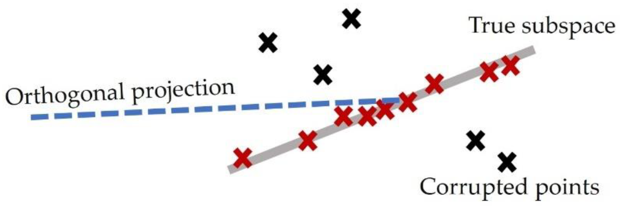
Figure 2.
Flowchart of online robust anomaly-detection procedure based on moving windows.

Figure 4.
Evolution of the six orders of natural frequencies of the KW51 bridge under temperature variability. Blue scatters highlight the sparse outlies observed below 0°C modal frequencies.
Figure 4.
Evolution of the six orders of natural frequencies of the KW51 bridge under temperature variability. Blue scatters highlight the sparse outlies observed below 0°C modal frequencies.
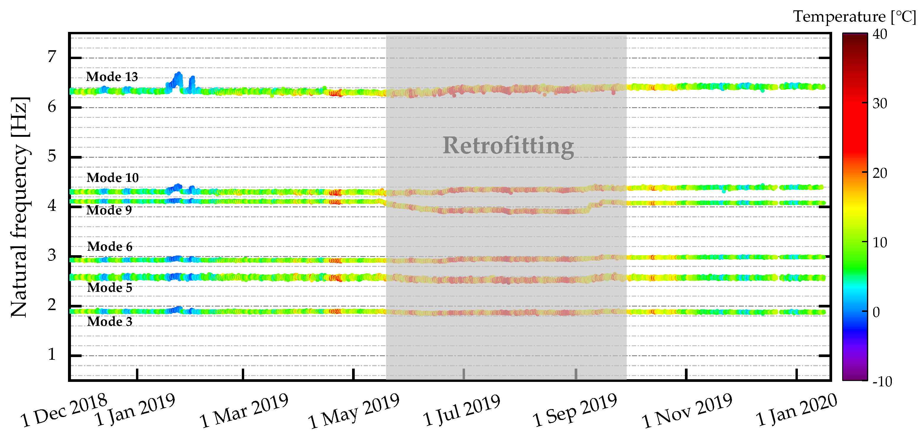
Figure 5.
Novelty detection using the complete frequency dataset (Dataset 1) of the KW51 bridge without data normalization. The control-limit width was adjusted from 5 to 25.
Figure 5.
Novelty detection using the complete frequency dataset (Dataset 1) of the KW51 bridge without data normalization. The control-limit width was adjusted from 5 to 25.
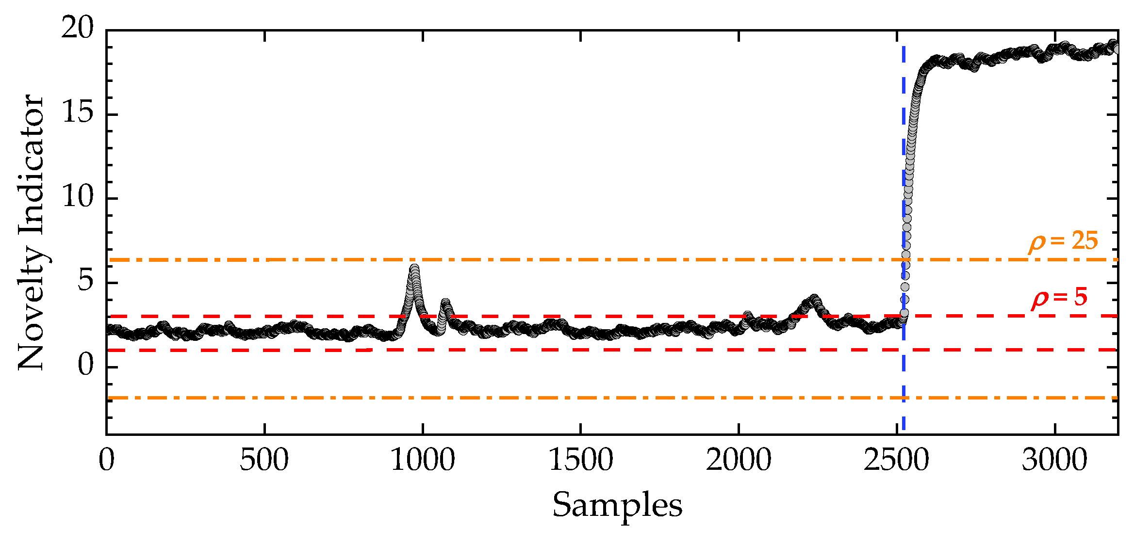
Figure 6.
OP-based residuals for the complete frequency dataset (Dataset 1). The blue dashed line separates the detection results before and after retrofitting.
Figure 6.
OP-based residuals for the complete frequency dataset (Dataset 1). The blue dashed line separates the detection results before and after retrofitting.
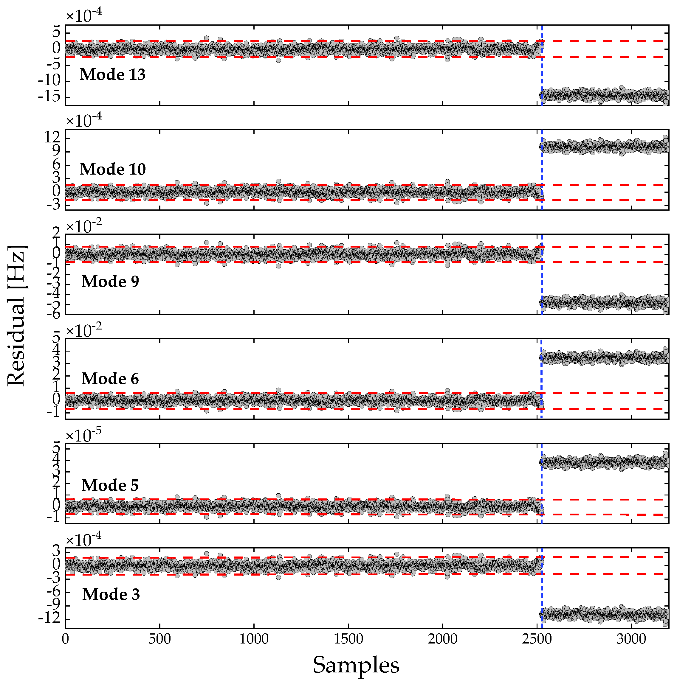
Figure 7.
Novelty detection using the complete frequency dataset (Dataset 1) based on the proposed anomaly-detection procedure. The control-limit width was set to 5. The subgraph illustrates the timeliness of anomaly detection.
Figure 7.
Novelty detection using the complete frequency dataset (Dataset 1) based on the proposed anomaly-detection procedure. The control-limit width was set to 5. The subgraph illustrates the timeliness of anomaly detection.
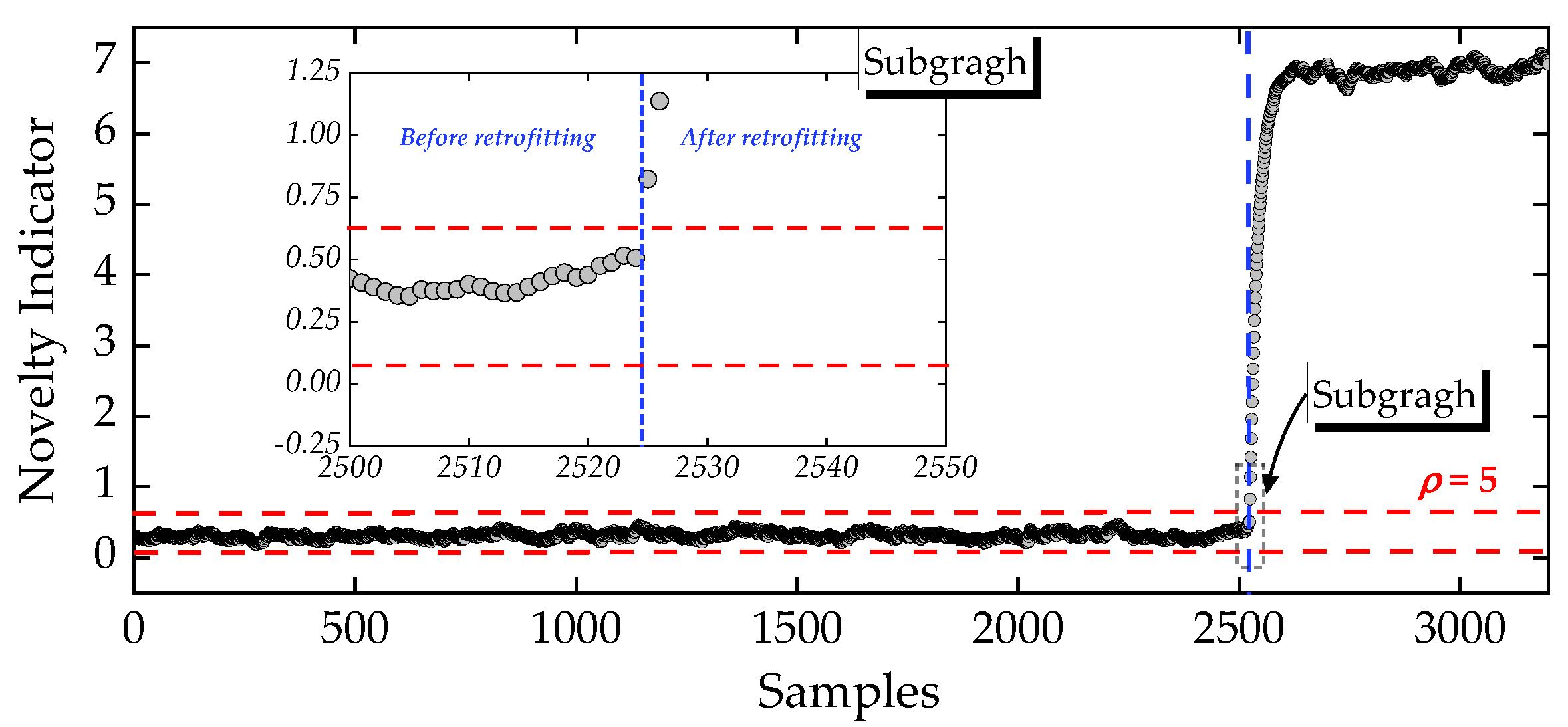
Figure 8.
NLRMC-based data cleansing/recovery of missing entries on mode 10, illustrated through (a) a global view and (b) a local view.
Figure 8.
NLRMC-based data cleansing/recovery of missing entries on mode 10, illustrated through (a) a global view and (b) a local view.
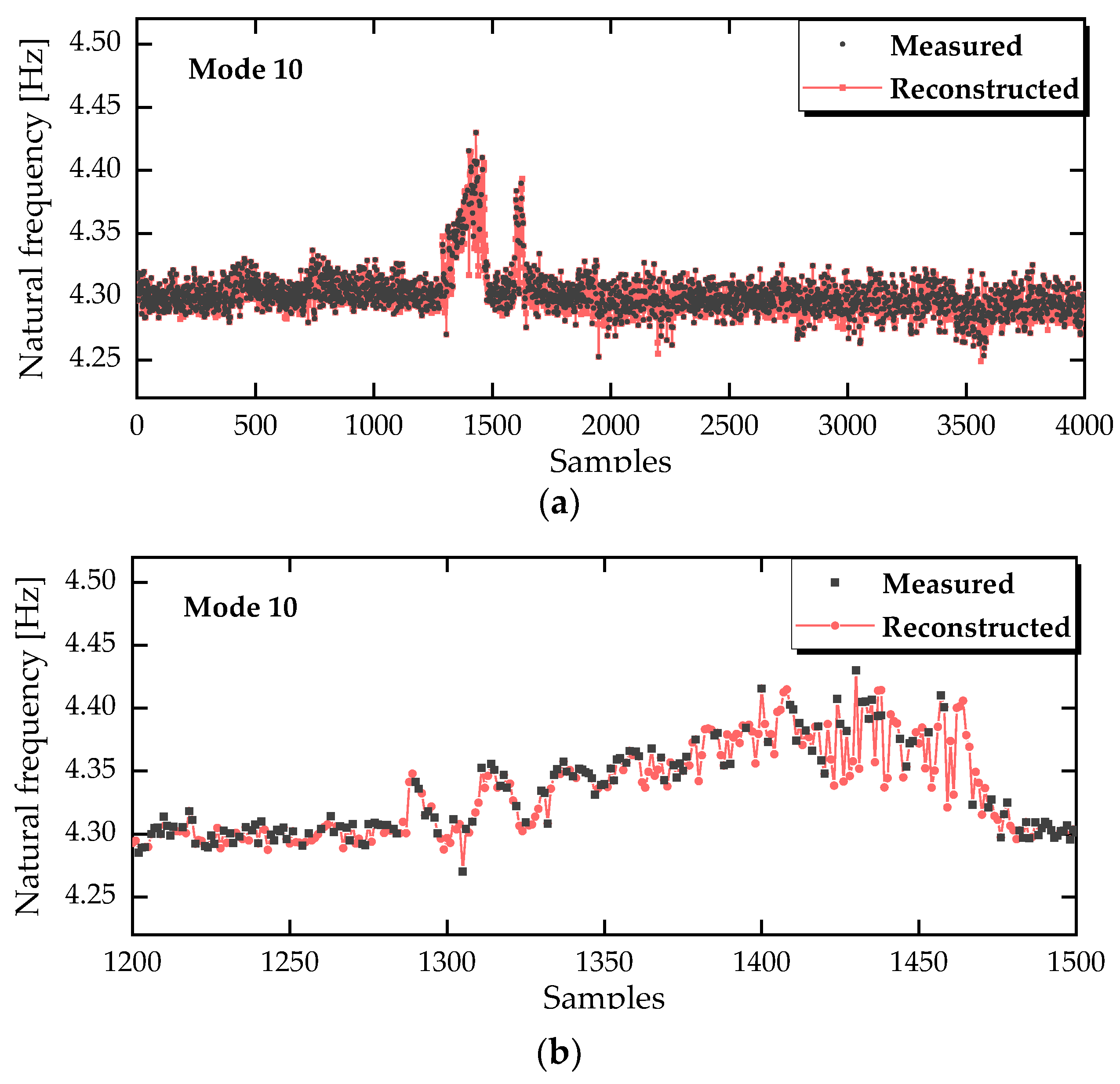
Figure 9.
OP-based residuals for the incomplete frequency dataset (Dataset 2). The blue dashed line separates the detection results before and after retrofitting.
Figure 9.
OP-based residuals for the incomplete frequency dataset (Dataset 2). The blue dashed line separates the detection results before and after retrofitting.
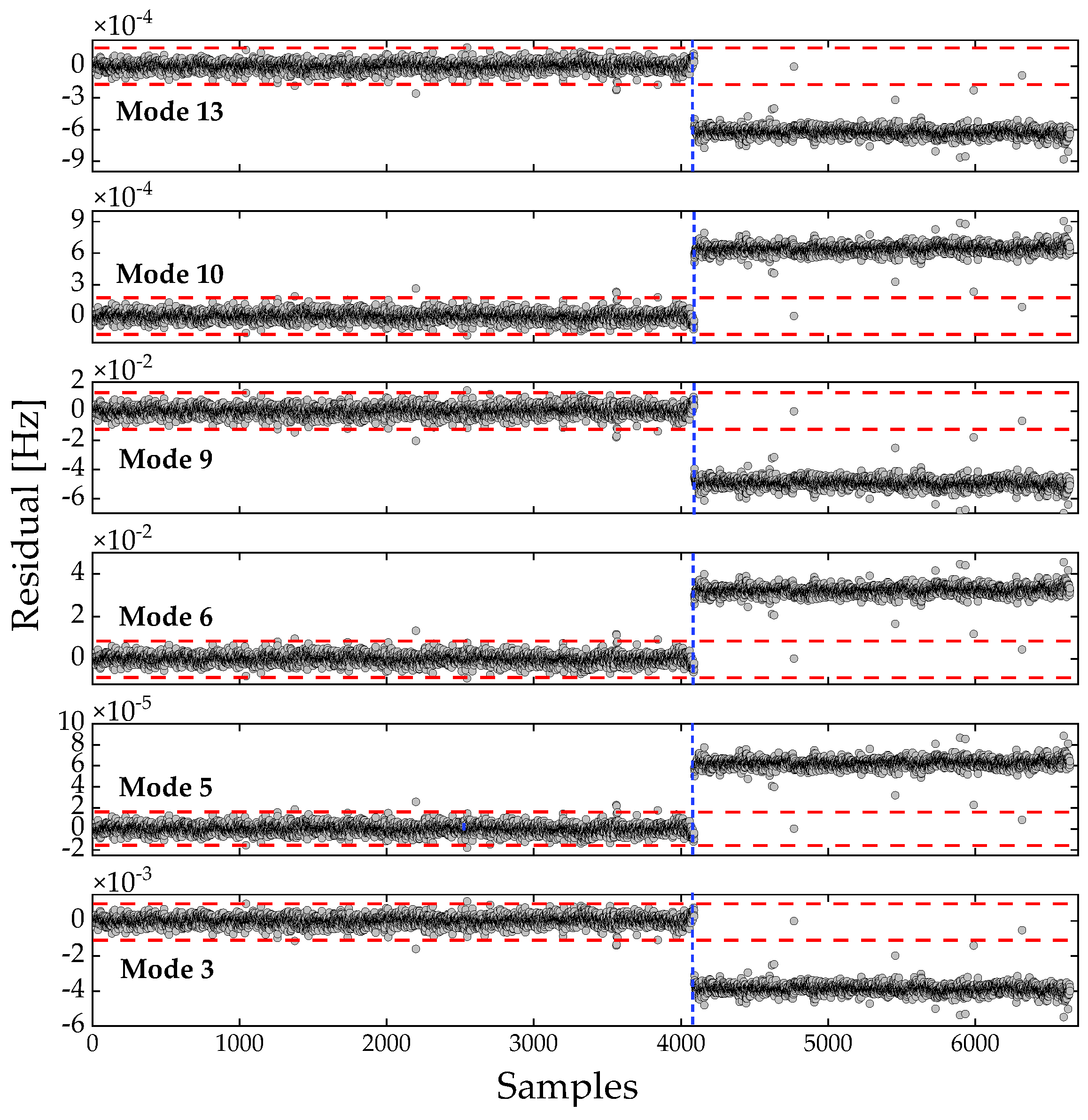
Figure 10.
Novelty detection using the incomplete frequency dataset (Dataset 2) based on the proposed anomaly-detection procedure. The control-limit width was set to 5. The subgraph illustrates the timeliness of anomaly detection.
Figure 10.
Novelty detection using the incomplete frequency dataset (Dataset 2) based on the proposed anomaly-detection procedure. The control-limit width was set to 5. The subgraph illustrates the timeliness of anomaly detection.
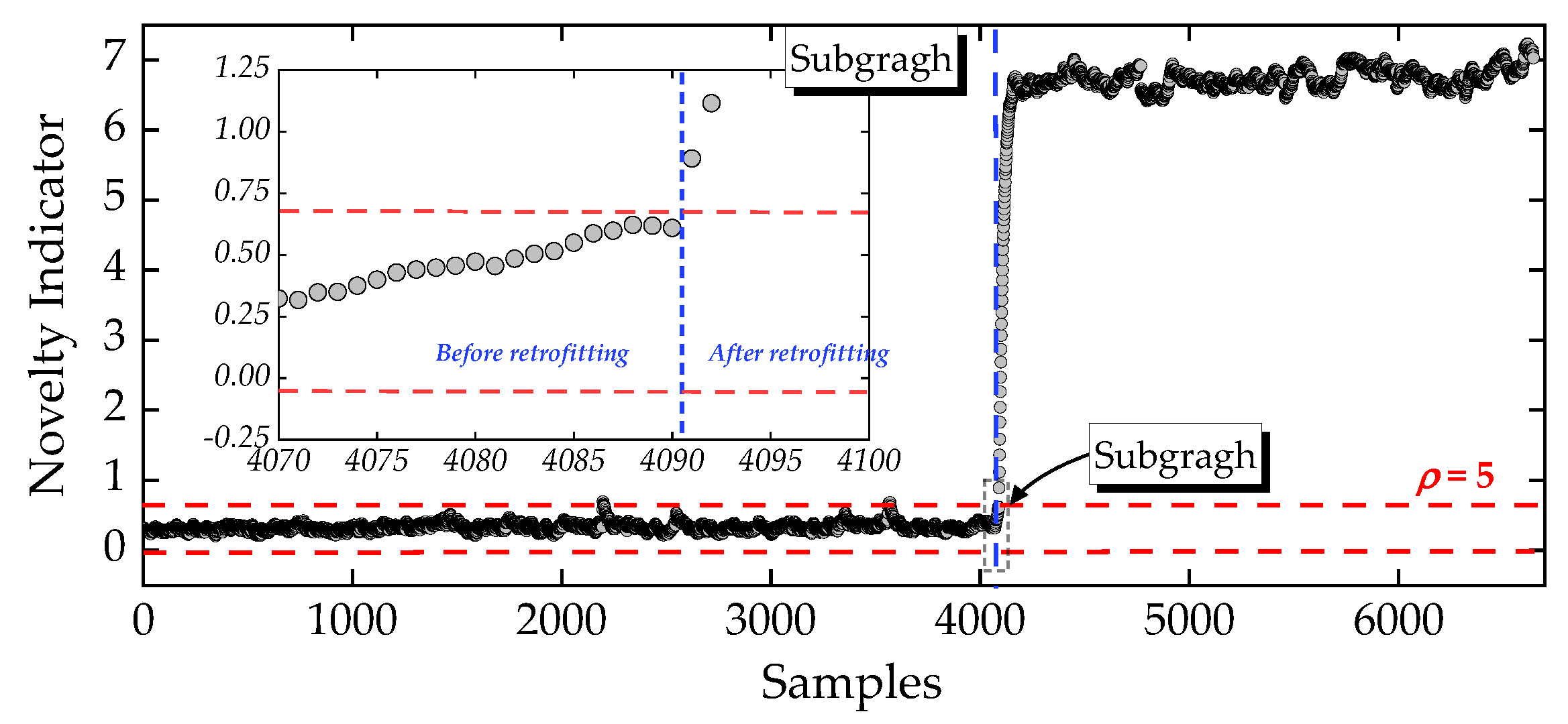

Table 1.
SR (identification success rate) and UR (data utilization rate of the corresponding frequency datasets) of modes considered for approach’ s validation.
Table 1.
SR (identification success rate) and UR (data utilization rate of the corresponding frequency datasets) of modes considered for approach’ s validation.
| Mode No. | SR [%] |
UR [%] (Dataset 1) |
UR [%] (Dataset 2) |
| 3 | 95.5 | 49.7 | 100 |
| 5 | 88.9 | 53.4 | 100 |
| 6 | 98.1 | 48.4 | 100 |
| 9 | 97.8 | 48.5 | 100 |
| 10 | 52.4 | 90.6 | 100 |
| 13 | 89.2 | 53.2 | 100 |
Disclaimer/Publisher’s Note: The statements, opinions and data contained in all publications are solely those of the individual author(s) and contributor(s) and not of MDPI and/or the editor(s). MDPI and/or the editor(s) disclaim responsibility for any injury to people or property resulting from any ideas, methods, instructions or products referred to in the content. |
© 2025 by the authors. Licensee MDPI, Basel, Switzerland. This article is an open access article distributed under the terms and conditions of the Creative Commons Attribution (CC BY) license (http://creativecommons.org/licenses/by/4.0/).
Copyright: This open access article is published under a Creative Commons CC BY 4.0 license, which permit the free download, distribution, and reuse, provided that the author and preprint are cited in any reuse.


