
Submitted:
02 April 2025
Posted:
07 April 2025
You are already at the latest version
Abstract
This study investigates the use of Deep Belief Networks (DBNs) for classifying structural states in Structural Health Monitoring (SHM) systems. Dimensionality reduction techniques—such as Principal Component Analysis (PCA) and t-SNE—enabled a clear separation between pre- and post-retrofitting conditions, emphasizing the DBN’s ability to capture relevant classification features. Compared to unsupervised approaches such as K-means and PCA, DBNs demonstrate superior discrimination and generalization capabilities by leveraging multiple layers of Restricted Boltzmann Machines (RBMs) to extract richer data representations. Experimental results confirm the model’s ability to detect complex patterns in large datasets, achieving median cross-validation accuracies of 98.04% for ambient data and 96.96% for train data, with low variability. While DBNs perform slightly below the Random Forest model in ambient data classification (99.19%), they surpass it when handling more complex signals such as train data (95.91%). Noise robustness analysis indicates acceptable tolerance, maintaining over 90% accuracy for ambient data at noise levels σnoise≤0.5, though accuracy declines significantly under extreme noise conditions. Comparisons with previous SHM research confirm the competitive performance of DBNs, often exceeding results from CNN and LSTM models. These findings support DBNs as a promising and reliable approach for SHM applications. Future research should aim to enhance noise resilience and improve performance under imbalanced data conditions, further promoting DBNs as a robust tool for data-driven structural assessment and infrastructure monitoring.
Keywords:
deep belief networks
; structural health monitoring
; unsupervised learning
; PCA
; t-SNE
; classification
; robustness
; cross-validation
; noise analysis
; inverse problems
1. Introduction
Some globally recognized accidents, such as those of the Tacoma Bridge (Tacoma, 1940), Morandi Bridge (Genoa, 2018), or FIU Bridge (Florida, 2018), have driven the adoption of Structural Health Monitoring (SHM) techniques in civil engineering, which allows for early damage detection and the implementation of corrective measures before catastrophic failures occur [1].
Retrofitting, or structural reinforcement, plays a key role in SHM by enhancing the strength and durability of existing structures [2]. SHM facilitates the identification of specific areas requiring reinforcement, optimizing resource allocation and improving intervention effectiveness. A notable example is the monitoring of the KW51 railway bridge, where continuous SHM throughout the reinforcement process allowed for a detailed assessment of the interventions’ impact [3].
The integration of artificial intelligence (AI) and machine learning (ML) techniques has significantly enhanced SHM by enabling the real-time analysis of large datasets collected through sensor networks. AI-driven models, including deep learning and ensemble approaches, have improved both damage detection accuracy and the effectiveness of predictive maintenance planning [4,5,6].
Recent studies have demonstrated that deep learning techniques can automate structural damage identification with high precision [7]. Additionally, AI-powered smart sensors support the shift from reactive interventions to predictive maintenance, thereby improving infrastructure reliability [8]. For instance, Mansouri et al. (2024) developed a Bluetooth-based strain gauge sensor network capable of detecting and localizing cracks in real time, showcasing the potential of ML for continuous structural assessment [9]. These AI-driven approaches collectively enhance infrastructure safety and maintenance strategies, emphasizing the importance of integrating SHM and ML to ensure long-term structural resilience.
However, the performance of ML models strongly depends on the quality and quantity of the available data, as insufficient or low-quality datasets can significantly reduce predictive accuracy [10,19]. In particular, high data dimensionality and the presence of noise contribute to increased uncertainty in model predictions.
To mitigate these limitations, Presno et al. [11] employed a Random Forest (RF) classifier trained in the spectral domain to predict the effect of retrofitting on the KW15 railway bridge [1], using both ambient and train-induced accelerometer data. The RF classifier achieved an accuracy of and an AUC of when using ambient data. To explore the influence of stronger excitation, the study examined whether train passages would enhance predictive performance. Despite high classification accuracy, a performance drop was observed with train-induced data. This reduction was attributed to the size imbalance between the datasets, as the ambient dataset was approximately 50 times larger than the train dataset.
In ambient data, low-frequency components were the most effective in distinguishing retrofitting effects. Interestingly, certain modal frequencies in the range of Hz showed comparable discriminative power to the primary low frequencies ( Hz and Hz). In contrast, for train data, the discriminative strength of frequencies followed a natural order based on their Fisher Ratio: low frequencies were most affected by train-induced vibrations, with decreasing influence observed at medium and high frequencies.
In this article, we compare the results previously presented in [11] with those obtained using a Deep Learning classifier, applied to both ambient and train-induced data.
Deep Belief Networks (DBNs) [12] offer several advantages for SHM applications. These include unsupervised pretraining, effective weight initialization that facilitates convergence, automatic extraction of high-level features that enhance classification performance, and robustness to noise through probabilistic modeling. Collectively, these properties allow DBNs to generalize better than fully supervised deep networks. Their ability to model complex patterns makes them particularly suitable for SHM tasks.
Kamada et al. [13] introduced an Adaptive Structural Learning approach using DBNs for image-based crack detection in concrete structures. By incorporating Adaptive Restricted Boltzmann Machines, their method significantly improved crack identification and classification, demonstrating the potential of DBNs for automating damage detection and advancing SHM techniques.
Moreover, DBNs can learn meaningful feature representations even in the absence of large labeled datasets. This characteristic is particularly valuable in SHM, where labeled data may be limited—especially during the early stages of monitoring.
2. Materials and Methods
Data were collected on the KW15 railway bridge, located in Leuven, Belgium, which connects the towns of Herent (km 2.3) and Leuven (km 2.2). This steel bridge, operational since 2003, accommodates both railway and vehicular traffic on its lower level. It has a total length of 115 meters and a width of 12.4 meters.
The dataset used in this study was obtained using 12 uniaxial accelerometers—six positioned on the bridge deck and six on the arches—recording acceleration signals as trains passed in either direction. Monitoring began on October 2, 2018, and concluded on January 15, 2020, covering the entire retrofitting period. Acceleration measurements started 10 seconds before a train entered the bridge and continued for 30 seconds after it exited. The data collection was divided into three phases: (i) before the reinforcement (October 2, 2018 – May 15, 2019), (ii) during the reinforcement (May 15, 2019 – September 27, 2019), and (iii) after the reinforcement (September 27, 2019 – January 15, 2020). If a sensor was inactive or malfunctioning, its data were replaced with "NaN" values. The retrofitting involved reinforcement of the joints between the bridge deck and the arches to enhance structural safety, addressing stability concerns identified during construction [1].
Retrofitting refers to the process of strengthening or modifying a structure—or parts of it—to improve its durability. This technique is frequently used to increase resilience against environmental effects, aging, or deficiencies in design and construction. In this case, it is assumed that the bridge exhibited structural deficiencies prior to retrofitting, which were addressed through reinforcement. Therefore, data recorded before the intervention reflect a structurally deficient state, whereas data collected afterward correspond to a structurally sound condition.
The main objective of this study is to compare the results obtained from ambient data with those derived from non-ambient (train-induced) data. This comparison aims to evaluate whether signals recorded under significant loading conditions, such as train passages, provide greater discriminatory power than signals captured in the absence of such loading. The methodology used follows the framework established in [11], as illustrated in Figure 1.
Figure 2 shows four types of acceleration signals collected by the sensors: before and after retrofitting, as well as ambient and non-ambient (train) data. Notably, the maximum amplitude of the acceleration data recorded before retrofitting (before-train) is more than twice as high as that observed after retrofitting (after-train). However, the post-retrofitting data exhibits a more homogeneous amplitude, while the before-train data contains a central region with lower amplitude. The number of data points recorded before retrofitting in the non-ambient case is 4232, while after retrofitting it is 4968, approximately 50 times fewer than the ambient dataset. Furthermore, compared to ambient data (recorded in the absence of a passing train), the amplitude of before-train data is 750 times greater, whereas post-retrofitting, this excess amplitude is reduced by a factor of around 150.
Signals are transformed from the time domain to the frequency domain using Power Spectral Density (PSD) analysis. The Welch PSD method offers insights into the contribution of each frequency to the total power of the signal [14]. The frequencies used in the PSD calculations correspond to the bridge’s modal frequencies, aiming to identify how these frequencies contribute to the vibration energy, thereby revealing the natural oscillation patterns of the bridge. Additionally, the PSD facilitates the comparison of different measurements, helping to detect behavioral changes in the bridge and assess potential causes of failure by analyzing shifts in the contribution of these frequencies to the overall vibration energy.
As in the study of ambient data, once the accelerometer data (before-train and after-train) is processed, any NaN values are removed, and the Welch PSD is computed for the 14 modal frequencies published in [3]. It is assumed that the bridge exhibited structural faults prior to the retrofitting, which were addressed after the renovations.
2.1. Deep Belief Network (DBNs) and Restricted Boltzmann Machines (RBMs)
Deep Belief Networks (DBNs) are built on probabilistic graphical models, unsupervised learning, and neural networks. They consist of multiple layers of Restricted Boltzmann Machines (RBMs), which learn probabilistic data representations.
DBNs are trained in two stages: first, RBMs undergo unsupervised pretraining to capture hierarchical features, followed by supervised fine-tuning for classification or regression tasks [12,15]. Mathematically, each layer models a conditional probability distribution over the previous one.
This hierarchical structure allows DBNs to learn increasingly abstract representations: lower layers capture basic features, while upper layers extract high-level patterns. The network forms a directed acyclic graph, where upper layers act as a generative model and lower layers as a discriminative network. This hybrid nature enables DBNs to effectively model complex data relationships, leveraging the strengths of RBMs and deep neural networks.
Restricted Boltzmann Machines (RBMs)
A Restricted Boltzmann Machine (RBM) consists of two units:
- -
- A set of m visible layers (), representing the input data. The notation means that the vector is a binary vector of dimension m, that is, a set of m elements where each element can be either 0 or 1.
- -
- A set of n hidden layers (): representing the learned representations of the input data.
- -
- and are the activations (0 or 1) of the visible and hidden units. In a RBMs there are no connections between units within the same layer. The units in the visible and hidden layers are connected by weights.
The energy of a particular state in an RBM can be written as [16]:
where and are the bias vectors for the visible and hidden layers and represents the weight between visible unit and hidden unit .
The joint probability of a configuration can be written as:
where K is a normalization factor for P to be a probability.
The network optimization tries to minimize this energy function to learn a plausible representation of the data. This is equivalent to maximizing the probability of the configuration. Learning in an RBM is based on adjusting the weights W, the visible biases , and the hidden biases to maximize the logarithmic probability of the input data. This task is called the training of the RBM.
This is done using the contrastive divergence (CD) method. In CD, the gradient of the log-probability with respect to the weights is given by:
where denotes the expectation over the empirical data distribution, and represents the expectation under the distribution defined by the RBM [12,17].
A DBN is built by stacking multiple RBMs hierarchically [18]. After training an initial RBM to model the distribution of the input data, the activations of the hidden units are used as input to train the next RBM. This process is repeated for all layers, allowing each level to learn progressively more abstract representations. Mathematically, if represents the hidden units of layer k, then:
whare and are the weights and biases of layer k, and
is the element-wise sigmoid function.
After pretraining the layers, the RBMs are assembled into a DBN for supervised tasks. The supervised model adds an output final layer F that predicts the labels using the learned latent representations:
where represents the DBN forward model, are the inputs, and and are the results of the binary cross-entropy loss function optimization:
3. Results
This section aims to compare retrofitting predictions via DBNs using ambient and train data, highlighting their main similarities and differences. Specifically, the study assesses the discriminatory power of train data relative to ambient data. A key distinction between these datasets is that train data not only lacks an equal number of measurements before and after retrofitting but also contains 50 to 58 times fewer measurements than ambient data.
The signals are analyzed in the frequency domain by computing the power spectral density (PSD) at the bridge’s 14 modal frequencies. Presno et al. [11], conducted a study on the discriminatory power of these frequencies, concluding that monitoring the bridge’s natural vibration modes is optimal for predicting the effect of retrofitting.
To train and test the machine learning models we used the values of , where represents the array of modal frequencies, categorized into two groups:
- -
- Ambient data: Class 1, comprising 14864 measurements recorded before retrofitting, and Class 2, consisting of 16272 measurements taken afterward.
- -
- Train data: Class 1, comprising 4232 measurements recorded before retrofitting, and Class 2, consisting of 4968 measurements taken afterward.
3.1. Discriminatory Frequencies for Ambient and Train Data
The Fisher ratio of the data is calculated in order to determine which features (modal frequencies) are most effective for distinguishing between the data before and after retrofitting, as explained in [11]. A high ratio value indicates that the difference between the means of the two classes is large compared to the variability within each class, meaning that this feature is good for differentiating between the two conditions.
Figure 3 represents the values of the Fisher ratio of at the 14 modal frequencies, for both, ambient and train data. It can be observed that in the case of ambient data (Figure 3a) the values of the Fisher ratio do not decrease with increasing modal frequencies. The maximum value of the Fisher ratio is slightly above , and there are 5 modal frequencies for which the Fisher ratio is above the mean, corresponding to , , , , and Hz.
A substantial difference in the case of train data is that the modal frequencies appear ordered according to the decreasing Fisher ratio, from lower to higher frequency values (see Figure 3b). Another difference is that there are no frequencies with Fisher ratios above the mean within frequency intervals where Fisher ratios have values below the mean, that is, only the first five frequencies seems to be discriminatory of the retrofitting effect.
To provide additional insight into the discriminatory power of the modal frequencies, Figure 4 presents the combined histograms of before and after retrofitting for both ambient and train data. As expected, the less discriminative frequencies in the ambient data exhibit greater overlap and/or higher variability in their distributions. In the train data, the higher, less discriminative frequencies show a more Gaussian distribution with lower variability, while the more discriminative frequencies display greater variability.
The boxplot provides a quick view of data dispersion and compares before and after retrofitting for both ambient and train data. For ambient data, [11] showed that the distribution range shifts from before retrofitting to a narrower interval post-retrofitting . This aligns with initial accelerometer signals, confirming that retrofitting effectively reduced structural vibrations.
Figure 5 show the boxplots before and after retrofitting for train data. It can be observed that the median values of after retrofitting also fall within a narrower range than before retrofitting. Also, the distribution range reduced from to post-retrofitting, which is significantly higher in magnitude compared to ambient data.
3.2. Unsupervised PCA Analysis and t-SNE
For both ambient and train data, principal component analysis (PCA) reveals the discriminatory power of the 14 modal frequencies, allowing dimensionality reduction without significant information loss, as shown in [11].
Figure 6 presents the projections of in 2- and 3-dimensional PCA subspaces for ambient and train data by using the the three most discriminative modal frequencies in each case. For ambient data, the three most discriminative modal frequencies are , , and . The first PCA explains of the variance, and two components account for . Five components are needed to exceed of the variance. For train data, the most discriminative frequencies are , , and . The first PCA explains only of the variance. Three components reach , five exceed , and nine are required for of the variance, indicating higher complexity in the case of train data.
Figure 7 shows the t-SNE representation of the data, comparing the ambient (left) and train (right) datasets. t-SNE validates the effectiveness of the extracted features, assesses the discriminative power of each dataset, and complements the PCA dimensionality reduction, strengthening the robustness of the study’s classification approach. This technique reveals the structure of high-dimensional data in a two-dimensional space. In the ambient dataset, the data points are more dispersed, suggesting less clear separability between groups. In contrast, the train data set forms more distinct clusters, indicating a stronger grouping of similar patterns. The projection does not fully align with the cross-validation results, suggesting that predictions using DBNs are more complex and cannot be entirely explained by a 2D representation.
3.3. Unsupervised K-Means Classifier for Train Data
The K-means algorithm is used to divide the data set into two clusters of similar characteristics by minimizing the sum of the squared distances from each data point to the centroid of its cluster, as shown in [11] for the case of ambient data.
The confusion matrix of this classifier for train data turned to be
where represents the number of samples correctly classified as before retrofitting; represents the number of samples incorrectly classified as after retrofitting; represents the number of samples correctly classified as after retrofitting; and represents the number of samples incorrectly classified as before retrofitting. The accuracy achieved by this algorithm with the first 5 most discriminatory modal frequencies was , slightly higher than achieved with the ambient data. This suggests that train data has a greater discriminatory power in detecting the effect of retrofitting compared to ambient data, as it subjects the structure to a higher load.
The ratio represents the ability to correctly identify the samples before retrofitting. This ratio is in the case of train data compare to for ambient data. However, the ability to correctly identify the samples after retrofitting drops to for train data, which is still slightly higher than in the case of ambient data. It can be observed that there is a lack of ability to classify the data after retrofitting, due to simplicity of this classifier.
3.4. Random Forest Classifier
Presno et al. [11] used a Random Forest classifier [20] to predict the effect of the retrofitting by using ambient data () for both classes: before and after retrofitting. This algorithm achieved a median accuracy of with a nearly perfect receiver operating characteristic (ROC) curve. Also, the final model, tested on the entire dataset, achieved accuracy demonstrating its effectiveness in predicting retrofitting effects for other civil structures. For the training data, the algorithm attains a median accuracy of , reaching a final model accuracy of , close to that obtained in the case of ambient data.
3.5. Deep Belief Network (DBN) Classifier
The implemented procedure provides a complete pipeline for training and evaluating a Deep Belief Network (DBN). This model combines unsupervised layer-wise learning using Restricted Boltzmann Machines (RBM) with a supervised fine-tuning phase for classification tasks. Below, the step-by-step process is detailed, explaining its purpose and the mathematical foundations underlying each stage.
3.5.1. Data Loading and Preprocessing
The first stage consists of data loading and preprocessing. These data are divided into two sets: and , which are labeled as and , respectively. Subsequently, the data is combined into a single set X and normalized to ensure that each feature has zero mean and unit standard deviation. Finally, the data is split into training and test subsets:
In the next stage, unsupervised training is introduced using RBMs. A grid search for hyperparameters is also performed to optimize the model’s performance. The search evaluates different parameter configurations, such as the number of hidden units, the learning rate, and the number of epochs.
3.5.2. Hyperparameter Search
When tuning a Restricted Boltzmann Machine (RBM), several crucial parameters should be considered to optimize its performance:
- Number of Hidden Units: The number of hidden units (neurons) in the RBM determines the capacity of the model to learn complex features from the input data. Using too few hidden units may prevent the model from capturing the full complexity of the data. On the other hand, using too many hidden units can lead to overfitting and make the training process slower. Therefore, it is necessary to strike a balance between the complexity of the model and the fitting of the data.
- Learning Rate controls the step size at each iteration while updating the weights. It determines how much the model adjusts its weights based on the gradient. If the learning rate is too high, the training may become unstable or diverge. On the other hand, if the learning rate is too low, it could result in slow convergence or cause the model to get stuck in local minima. Typically, a value between and is used, although it may vary depending on the specific problem.
- Number of Training Epochs: This defines how many times the algorithm will iterate over the entire dataset. Using too few epochs can lead to underfitting, where the model fails to learn sufficient patterns from the data. Conversely, using too many epochs can cause overfitting, where the model memorizes the data instead of generalizing effectively.
- Batch Size: This refers to the number of samples processed in each training step. Smaller batches can provide a more precise gradient estimate, but they make the training process noisier. Larger batches offer smoother gradients but can result in slower convergence and require more memory. The adopted solution consists of using cross-validation to evaluate how well the model generalizes to unseen data.
The hyperparameter analysis explored various configurations for the number of layers, units, and learning rates according to the following variables:
-
Model Complexity
- –
- Number of layers:
- –
- Number of units per layer:
-
Learning rate
- –
-
Number of training epochs
- –
- Epochs per RBM layer:
- –
- Epochs per DBN layer:
-
Batch size: Cross-validation experiments were conducted with partitions.This analysis has shown that the optimal configurations were:
- –
- Number of layers: 4
- –
- Number of units per layer:
- –
- Learning rate:
- –
- Epochs per RBM layer: 10
- –
- Epochs per DBN layer: 100
The performance of a Deep Belief Network (DBN) strongly depends on the careful selection of hyperparameters. In this study, a grid search was performed to identify the optimal network configuration by evaluating key parameters, including the number of hidden units, learning rate, training epochs, and batch size [21]. The results indicate that a balanced architecture outperforms more complex configurations, which are more prone to overfitting. The best results obtained using 4 layers with 128 to 1024 units per layer. In this case, a learning rate of provided the best balance between speed and stability. It was observed that 10 epochs per layer in the pretraining phase using Restricted Boltzmann Machines (RBMs) and 100 epochs in the fine-tuning phase resulted in optimal performance. Additionally, a 5-fold cross-validation was performed to evaluate the model’s generalization ability.
3.5.3. Cross-Validation Results with Ambient and Train Data Using DBNs
After pretraining, the DBN is fine-tuned using a fully connected output layer with a sigmoid activation function to perform binary classification. The entire network is then trained end-to-end using binary cross-entropy loss and the Adam optimization algorithm, refining the RBM-learned features.
To ensure that this fine-tuning process leads to a model that generalizes well beyond the training data, cross-validation is employed as a key evaluation technique. Cross-validation ensures a robust evaluation of the model ensuring its ability to generalize to unseen data, and the results obtained demonstrate low variability between folds. The importance of this process lies in its ability to detect issues such as overfitting, where the model memorizes the training data without capturing general patterns. The used statistical descriptors of cross-validation were:
The training and testing sizes are as follows:
-
Ambient data:
- –
- Training size
- –
- Testing size
-
Train data:
- –
- Training size
- –
- Testing size
Table 1 shows the cross-validation results using the train and ambient datasets with 14 modal frequencies. Ambient Data achieves a higher mean accuracy () but with greater variability (), ranging from (Fold 1) to (Fold 3). In contrast, Train Data shows a lower mean accuracy (), indicating potential for improvement, but with more consistent results (), with accuracy values between (Fold 3) and (Fold 5). This suggests that while the model benefits from Ambient Data, its performance is more stable when trained on Train Data, albeit at a slightly lower accuracy.
To address this, an expanded feature set using 100 evenly distributed frequencies within the modal frequency range was evaluated, leading to a significant accuracy improvement, as shown in Table 2. The preselection of 14 modal frequencies, previously used without noticeable information loss in machine learning models [11], cannot be directly extended to DBN-based methods with unsupervised learning. In this case, incorporating a broader frequency range of 100 frequencies significantly enhanced the results.
To further validate this trend, tests were performed with 500 and 1000 equidistant frequencies within the same range. The mean accuracy for the training data reached with 500 frequencies and with 1000, both considerably higher than the obtained with 100 frequencies. This behavior suggests that DBNs require a highly dense parameterization in the feature space.
The Table 2 presents the cross-validation accuracy results for Ambient Data and Train Data, both evaluated using five folds with the first 100 frequencies. Ambient Data achieves a higher mean accuracy () but with greater variability (), with accuracy values ranging from (Fold 4) to (Fold 5). Train Data, on the other hand, shows a slightly lower mean accuracy () but with more consistent results (), with accuracy values between (Fold 1) and (Fold 3). These results suggest that while both datasets yield high accuracy, the model trained on Ambient Data achieves slightly better performance at the cost of increased variability, whereas Train Data offers more stable results.
The confusion matrices obtained after model evaluation on unseen test data, for ambient data () and train data () are:
Both matrices present a good balance between true positives and negatives revealing high sensitivity and specificity in classification.
The model is evaluated using metrics such as the ROC curve, which describes the relationship between the true positive rate (TPR) and the false positive rate (FPR):
The area under the curve (AUC) is calculated as:
where t stands for the False Positive Rate .
Figure 8 shows the AUC curve for the ambient and train data. The AUC is very high in both cases ( for ambient and for train).
Based on these results, there are no signs of overfitting, which would typically manifest as poor generalization. This is evident even though the model achieves high classification performance on both datasets.
3.5.4. Robustness to Noise
The robustness of the model against noise is also evaluated by adding Gaussian noise to the test data:
where represents the noise level. This evaluation analyzes how the model’s accuracy changes as the noise in the input data increases. In our case, the noise is added directly to the attributes, which are .
A noise-robust DBN improves generalization, enhances reliability in real-world noisy data, minimizes errors in inverse problems, and ensures adaptable, reliable models for optimization and machine learning.
Figure 9 shows the impact of noise on the model’s accuracy for ambient data (left) and train data (right). It can be observed that:
- Both graphs show a decreasing trend in accuracy as the noise level increases, indicating that the model’s performance deteriorates under noisier conditions. This decline is expected, as higher noise levels introduce more uncertainty, making it harder for the model to maintain high accuracy.
- The Ambient data accuracy fluctuates slightly, with a noticeable dip in the range , followed by a small increase before continuing to decline.
- The Train data appears more robust to noise, with a smoother and more gradual decline in accuracy. Even at higher noise levels, the performance does not degrade as sharply as in the Ambient data.
- The accuracy of the Train data remains relatively stable at first, with a slight fluctuation in the range , where it briefly increases before gradually declining. The decrease is steady, but a more noticeable drop occurs around , after which the accuracy stabilizes slightly.
- The Ambient data graph (left) exhibits a steeper decline in accuracy compared to the Train data graph (right). At the highest noise level, the accuracy for the ambient data drops to , whereas the train data maintains a slightly higher accuracy ( approximately).
Therefore, the DBN is more robust to noise in ambient data than in train data. This could be due to the larger dataset size for ambient data, helping the model generalize better, and a higher signal complexity for train data.
Figure 10 illustrates the accuracy progression during training and validation on both the ambient and training datasets. In both cases, the model shows proper convergence, indicating that the selected hyperparameters are suitable.
The graph presents the learning curve, showing the evolution of training and validation accuracy over 100 epochs. Initially, both accuracies (training and validation) increase rapidly, stabilizing around 0.975. The validation accuracy exhibits greater fluctuations, especially up to 30 epochs for the train data, but follows a trend similar to the training accuracy, indicating that the model generalizes well. The presence of fluctuations in validation accuracy suggests some variability in model performance, though it remains close to the training accuracy, indicating an overall good fit without severe overfitting.
4. Discussion
Authors should discuss the results and how they can be interpreted from the perspective of previous studies and of the working hypotheses. The findings and their implications should be discussed in the broadest context possible. Future research directions may also be highlighted.
5. Conclusions
This study demonstrates that Deep Belief Networks (DBNs) are an effective tool for classifying structural states in Structural Health Monitoring (SHM) systems.
The application of dimensionality reduction techniques, such as Principal Component Analysis (PCA) and t-SNE, enabled a clear separation between pre- and post-retrofitting data. This effective discrimination suggests that the features extracted by the DBN capture relevant information for classification, in line with previous findings using other methodologies.
Compared to unsupervised methods such as K-means and PCA, DBNs exhibited substantial improvements in both discrimination and generalization. The integration of multiple layers of Restricted Boltzmann Machines (RBMs) allowed the model to learn richer feature representations, which translated into superior performance in SHM scenarios. Experimental results confirm the model’s capacity to extract complex patterns from large datasets, achieving median cross-validation accuracies of 98.04% for ambient data and 96.96% for train data, with minimal variability across folds. These results highlight the model’s strong generalization ability, with no signs of overfitting.
The lower accuracy observed for train data is attributed to the smaller dataset size and higher complexity of the associated signals. Notably, DBNs appear to perform better when the number of input features is large. For ambient data, the DBN’s performance was slightly below that of the Random Forest (RF) model (99.19%), while for train data, the DBN slightly outperformed RF (95.91%). These findings indicate that although RF excels in classifying ambient data, DBNs are more suited to handling complex signals, such as those induced by train passages.
A key aspect addressed in this work is the model’s robustness to artificial noise. The experiments revealed that for noise levels with a standard deviation of , the model maintained an accuracy above 90% for ambient data. For train data, this threshold dropped to . While these results demonstrate acceptable tolerance to moderate noise, accuracy declines sharply under high-noise conditions, indicating that DBNs may be sensitive to extreme perturbations.
When comparing these results with prior studies in the SHM literature, DBNs exhibit comparable or superior performance. For instance, Li et al. [22] reported accuracy using CNNs and with LSTMs in image-based inspection of bridge components, while Tang et al. [23] achieved accuracies between and using various neural architectures for bridge weight and speed estimation. These comparisons reinforce the validity and applicability of DBNs as a reliable solution for SHM tasks.
In summary, the findings of this work highlight the potential of DBNs for data-driven structural assessment. Their implementation in real-world monitoring systems can offer more accurate and robust diagnostics of infrastructure conditions, contributing to improved asset management and preventive maintenance in civil engineering. Future research should focus on enhancing the model’s robustness to noise and optimizing its performance in scenarios involving unbalanced or highly complex data distributions.
Overall, this research provides a strong case for the adoption of machine learning approaches in SHM, laying the foundation for more efficient and reliable infrastructure management strategies.
Author Contributions
Conceptualization, A.P.V., Z.F.M. and J.L.F.M.; methodology, A.P.V., Z.F.M. and J.L.F.M.; software, A.P.V.; validation, A.P.V., Z.F.M. and J.L.F.M.; formal analysis, A.P.V., Z.F.M. and J.L.F.M.; investigation, A.P.V., Z.F.M. and J.L.F.M.; resources, A.P.V., Z.F.M. and J.L.F.M.; data curation, A.P.V., Z.F.M. and J.L.F.M.; writing—original draft preparation, A.P.V., Z.F.M. and J.L.F.M.; writing—review and editing, A.P.V., Z.F.M. and J.L.F.M.; visualization, Z.F.M., J.L.F.M.; supervision, Z.F.M., J.L.F.M.; project administration, Z.F.M. and J.L.F.M.; funding acquisition, Z.F.M. and J.L.F.M. All authors have read and agreed to the published version of the manuscript.
Conflicts of Interest
The authors declare no conflicts of interest.
Abbreviations
The following abbreviations are used in this manuscript:
| SHM | Structural Health Monitoring |
| DBN | Deep Belief Network |
| RBM | Restricted Boltzmann Machine |
| PCA | Principal Component Analysis |
| t-SNE | t-Distributed Stochastic Neighbor Embedding |
| PSD | Power Spectral Density |
| ROC | Receiver Operating Characteristic |
| CV | Cross-Validation |
| RF | Random Forest |
| SNR | Signal-to-Noise Ratio |
| ML | Machine Learning |
| AI | Artificial Intelligence |
| DL | Deep Learning |
References
- Maes, K.; Lombaert, G. Monitoring railway bridge KW51 before, during, and after retrofitting. J. Bridge Eng. 2021, 26(3), 04721001. [Google Scholar] [CrossRef]
- Omori Yano, M.; Figueiredo, E.; da Silva, S.; Cury, A.; Moldovan, I. Transfer Learning for Structural Health Monitoring in Bridges That Underwent Retrofitting. Buildings 2023, 13. [Google Scholar] [CrossRef]
- Maes, K.; Van Meerbeeck, L.; Reynders, E.P.B.; Lombaert, G. Validation of vibration-based structural health monitoring on retrofitted railway bridge KW51. Mech. Syst. Signal Process 2022, 165, 108380. [Google Scholar] [CrossRef]
- Altabey, W.A.; Noori, M. Artificial-Intelligence-Based Methods for Structural Health Monitoring. Appl. Sci. 2022, 12(24), 12726. [Google Scholar] [CrossRef]
- Plevris, V.; Papazafeiropoulos, G. AI in Structural Health Monitoring for Infrastructure Maintenance and Safety. Infrastructures 2024, 9, 225. [Google Scholar] [CrossRef]
- Farrar, C.; Worden, K. Structural Health Monitoring: A Machine Learning Perspective; John Wiley and Sons: 2012. [CrossRef]
- Azimi, M.; Eslamlou, A.D.; Pekcan, G. Data-Driven Structural Health Monitoring and Damage Detection through Deep Learning: State-of-the-Art Review. Sensors (Basel) 2020, 20(10), 2778. [Google Scholar] [CrossRef] [PubMed]
- Sargiotis, D. Transforming Civil Engineering with AI and Machine Learning: Innovations, Applications, and Future Directions. Int. J. Res. Publ. Rev. 2025, 6(1), 3780–3805. [Google Scholar] [CrossRef]
- Mansouri, T.S.; Lubarsky, G.; Finlay, D.; McLaughlin, J. Machine Learning-Based Structural Health Monitoring Technique for Crack Detection and Localisation Using Bluetooth Strain Gauge Sensor Network. J. Sens. Actuator Netw. 2024, 13(6), 79. [Google Scholar] [CrossRef]
- Malekloo, A.; Ozer, E.; AlHamaydeh, M.; Girolami, M. Machine learning and structural health monitoring overview with emerging technology and high-dimensional data source highlights. Struct. Health Monit. 2021, 21(4), 147592172110368. [Google Scholar] [CrossRef]
- Presno Vélez, A.; Fernández Muñiz, M.Z.; Fernández Martínez, J.L. Enhancing Structural Health Monitoring with Machine Learning for Accurate Damage Prediction. AIMS Math. 2024, 9(11), 30493–30514. [Google Scholar] [CrossRef]
- Hinton, G.; Osindero, S.; Teh, Y.W. A fast learning algorithm for deep belief nets. Neural Comput. 2006, 18(7), 1527–1554. [Google Scholar] [CrossRef] [PubMed]
- Kamada, S.; Ichimura, T.; Iwasaki, T. An Adaptive Structural Learning of Deep Belief Network for Image-based Crack Detection in Concrete Structures Using SDNET2018. In Proc. ICIP 2020. [CrossRef]
- Welch, P. The use of fast Fourier transform for the estimation of power spectra: A method based on time averaging over short, modified periodograms. IEEE Trans. Audio Electroacoust. 1967, 15(2), 70–73. [Google Scholar] [CrossRef]
- Fischer, A.; Igel, C. Training Restricted Boltzmann Machines: An Introduction. In Lecture Notes in Computer Science; Springer, 2014; Vol. 8357, pp. 39–78.
- Smolensky, P. Information processing in dynamical systems: Foundations of harmony theory. In Parallel Distributed Processing: Explorations in the Microstructure of Cognition, 1986, Vol. 1, pp. 194–281.
- Hinton, G. Training products of experts by minimizing contrastive divergence. Neural Comput. 2002, 14(8), 1771–1800. [Google Scholar] [CrossRef] [PubMed]
- Bengio, Y.; Lamblin, P.; Popovici, D.; Larochelle, H. Greedy Layer-Wise Training of Deep Networks. Adv. Neural Inf. Process. Syst. 2007, 19, 153–160. [Google Scholar]
- Lee, Y.; Kim, H.; Min, S.; et al. Structural damage detection using deep learning and FE model updating techniques. Sci. Rep. 2023, 13, 18694. [Google Scholar] [CrossRef]
- Li, Z.-J.; Adamu, K.; Yan, K.; Xu, X.-L.; Shao, P.; Li, X.-H.; Bashir, H. M. Detection of Nut–Bolt Loss in Steel Bridges Using Deep Learning Techniques. Sustainability 2022, 14. [Google Scholar] [CrossRef]
- Tang, Y.; Chen, Z.; Wang, K.; Li, H. Vehicle Load Identification Based on Bridge Response Using Deep Learning. J. Civ. Struct. Health Monit. 2024, 14. [Google Scholar] [CrossRef]
Figure 1.
Flow chart of the methodology.
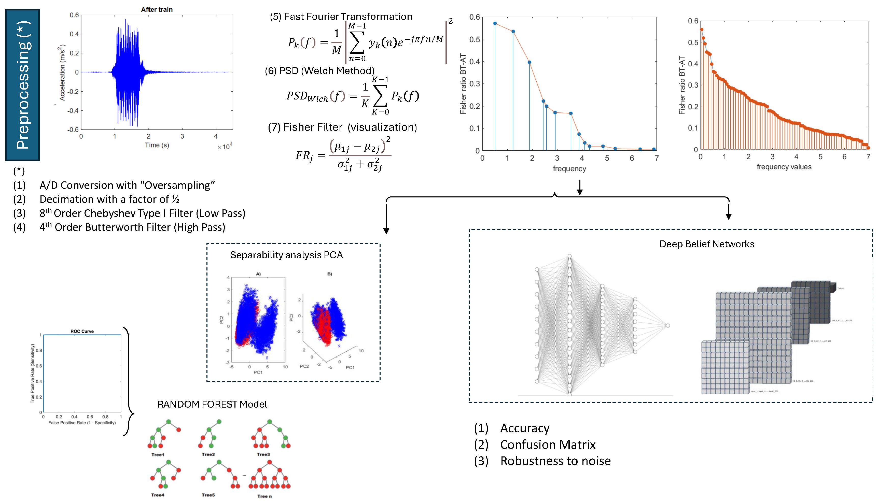
Figure 2.
Four types of signals collected by the accelerometers: before and after retrofitting under ambient and train excitation.
Figure 2.
Four types of signals collected by the accelerometers: before and after retrofitting under ambient and train excitation.
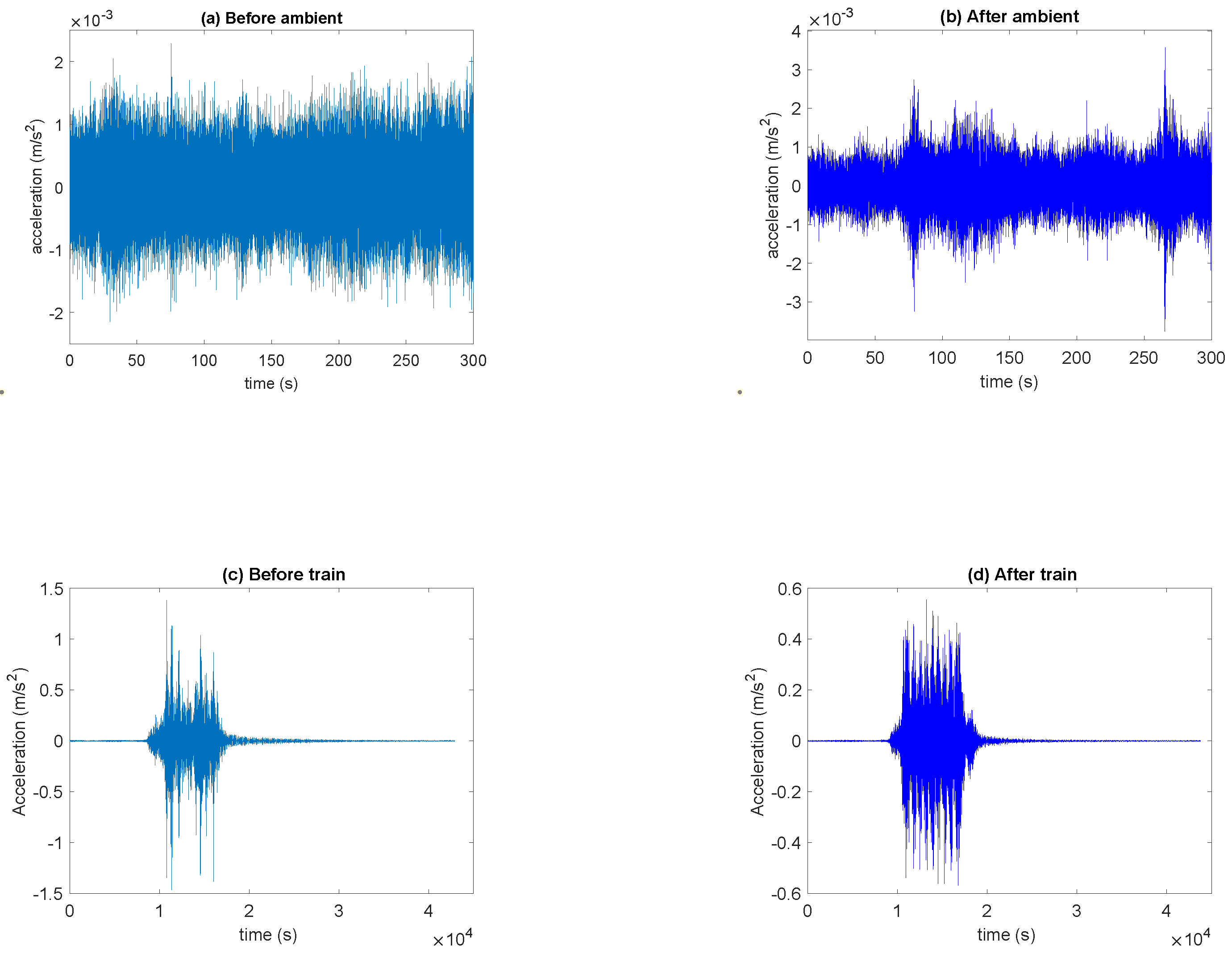
Figure 3.
Fisher ratio of Before and After retrofitting for: (a) Ambient data, (b) Train data.
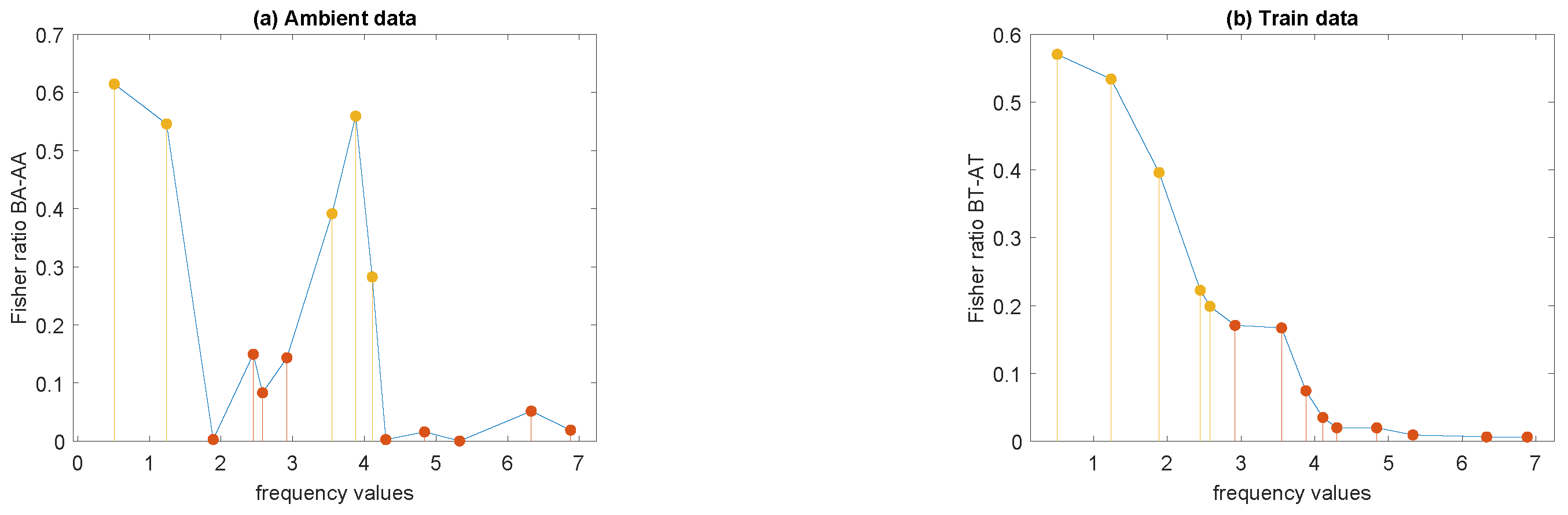
Figure 4.
Combined histogram of before and after retrofitting, considering modal frequencies arranged in ascending order from left to right and top to bottom. (a) Ambient data, (b) Train data.
Figure 4.
Combined histogram of before and after retrofitting, considering modal frequencies arranged in ascending order from left to right and top to bottom. (a) Ambient data, (b) Train data.
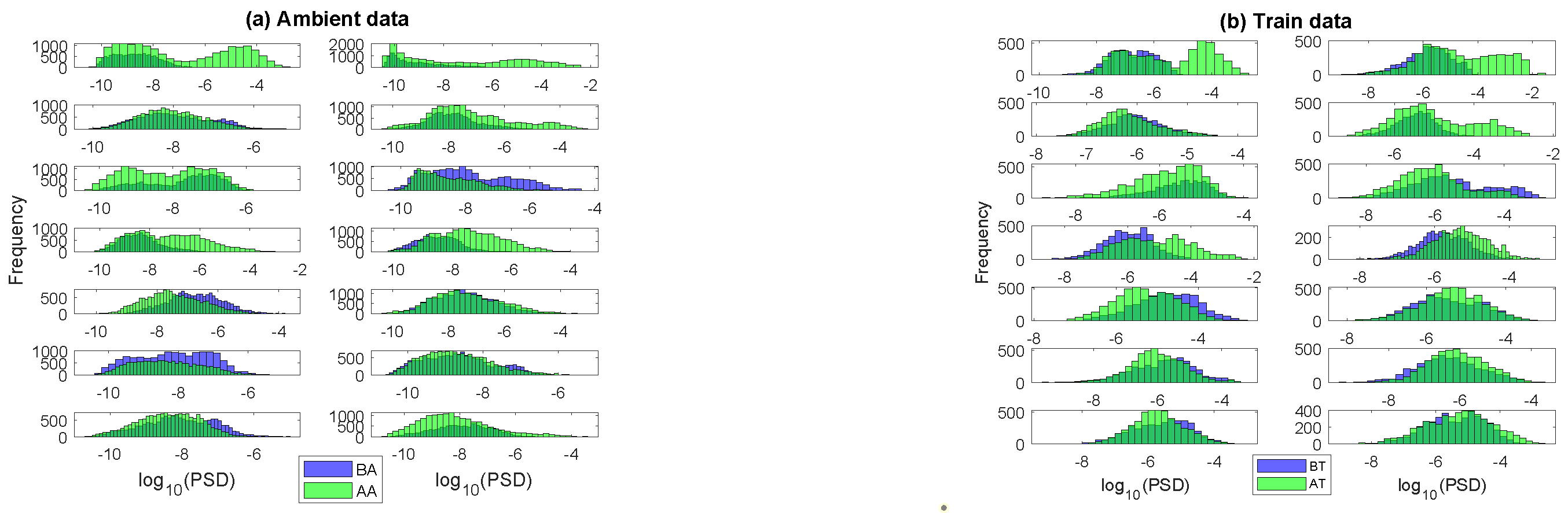
Figure 5.
Interquartile range of for train data at each modal frequency: (a) before retrofitting and (b) after retrofitting.
Figure 5.
Interquartile range of for train data at each modal frequency: (a) before retrofitting and (b) after retrofitting.
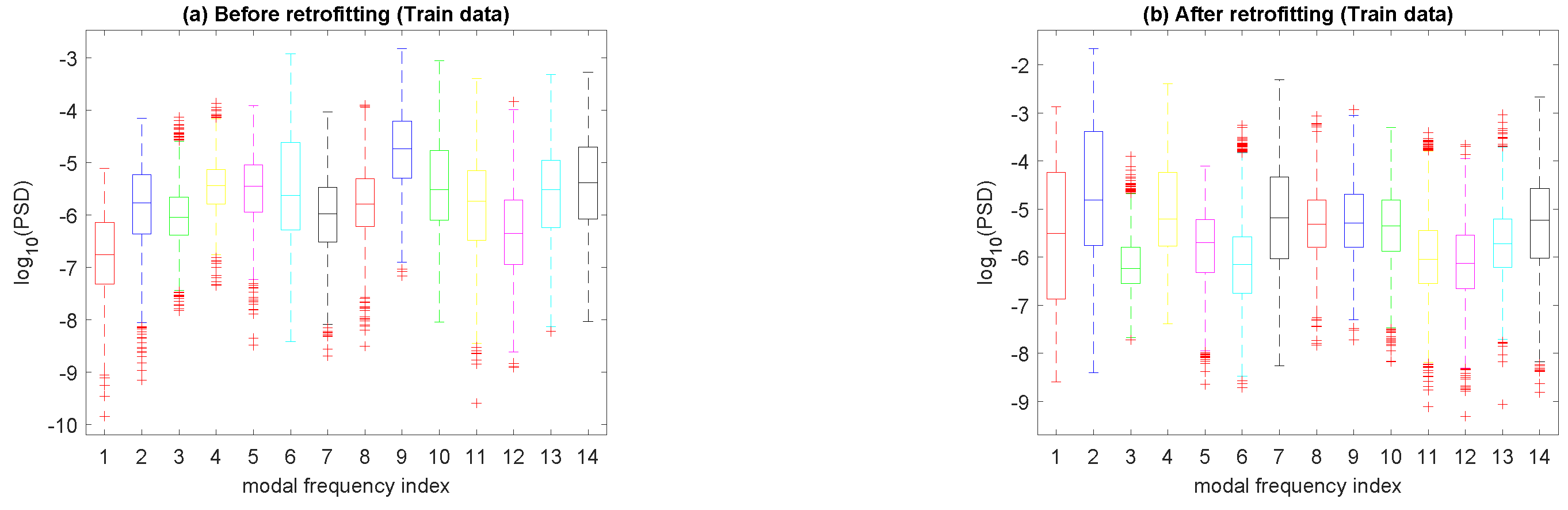
Figure 6.
Principal Components 1 and 2, and 1, 2 and 3 of before (red) and after (blue) retrofitting, respectively: (a) ambient data, (b) train data
Figure 6.
Principal Components 1 and 2, and 1, 2 and 3 of before (red) and after (blue) retrofitting, respectively: (a) ambient data, (b) train data
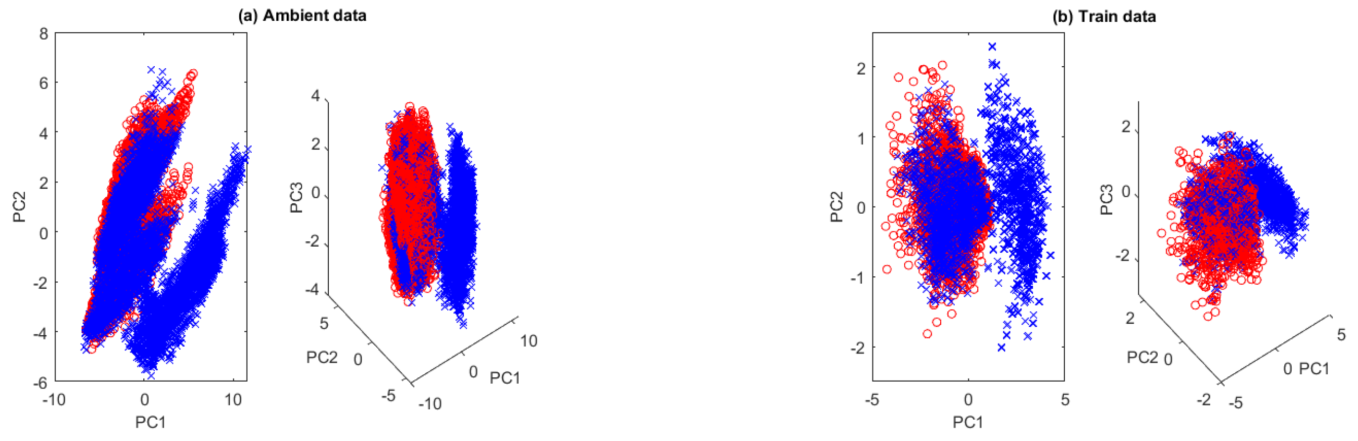
Figure 7.
t-SNE visualization of (a) Ambient data and (b) Train data.
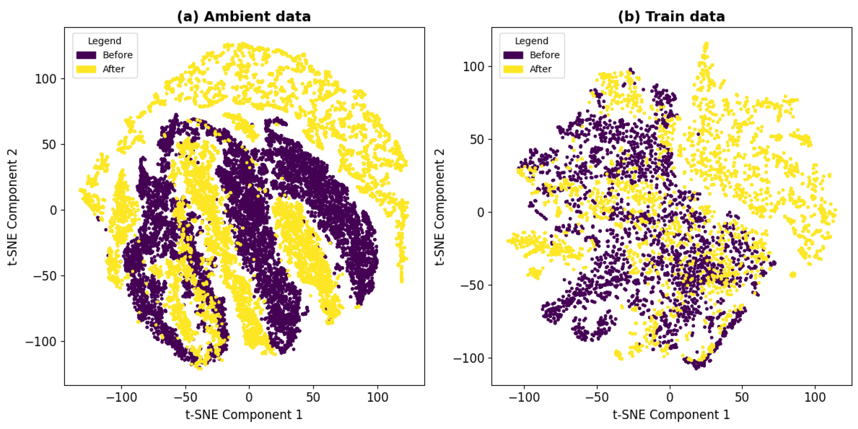
Figure 8.
Receiver Operating Characteristic (ROC) curves.
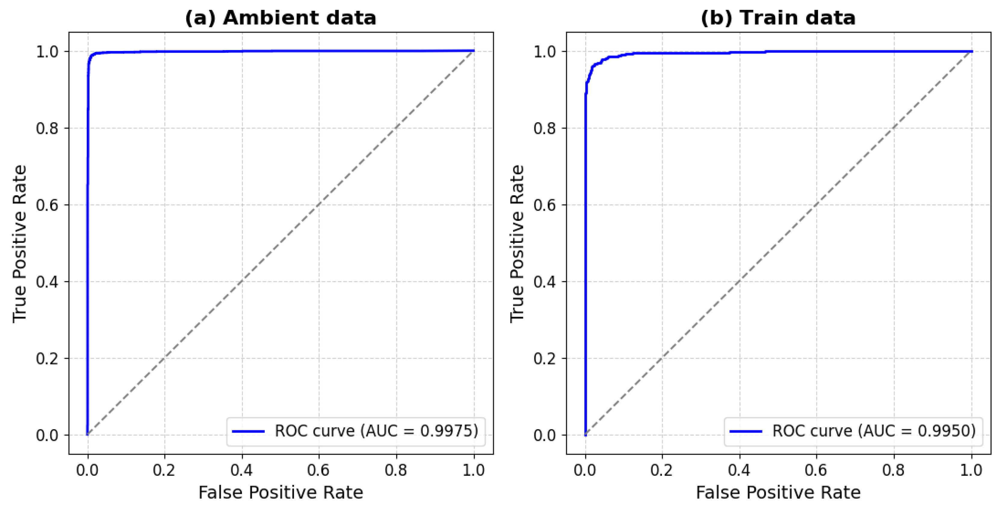
Figure 9.
Robustness to noise on model accuracy.
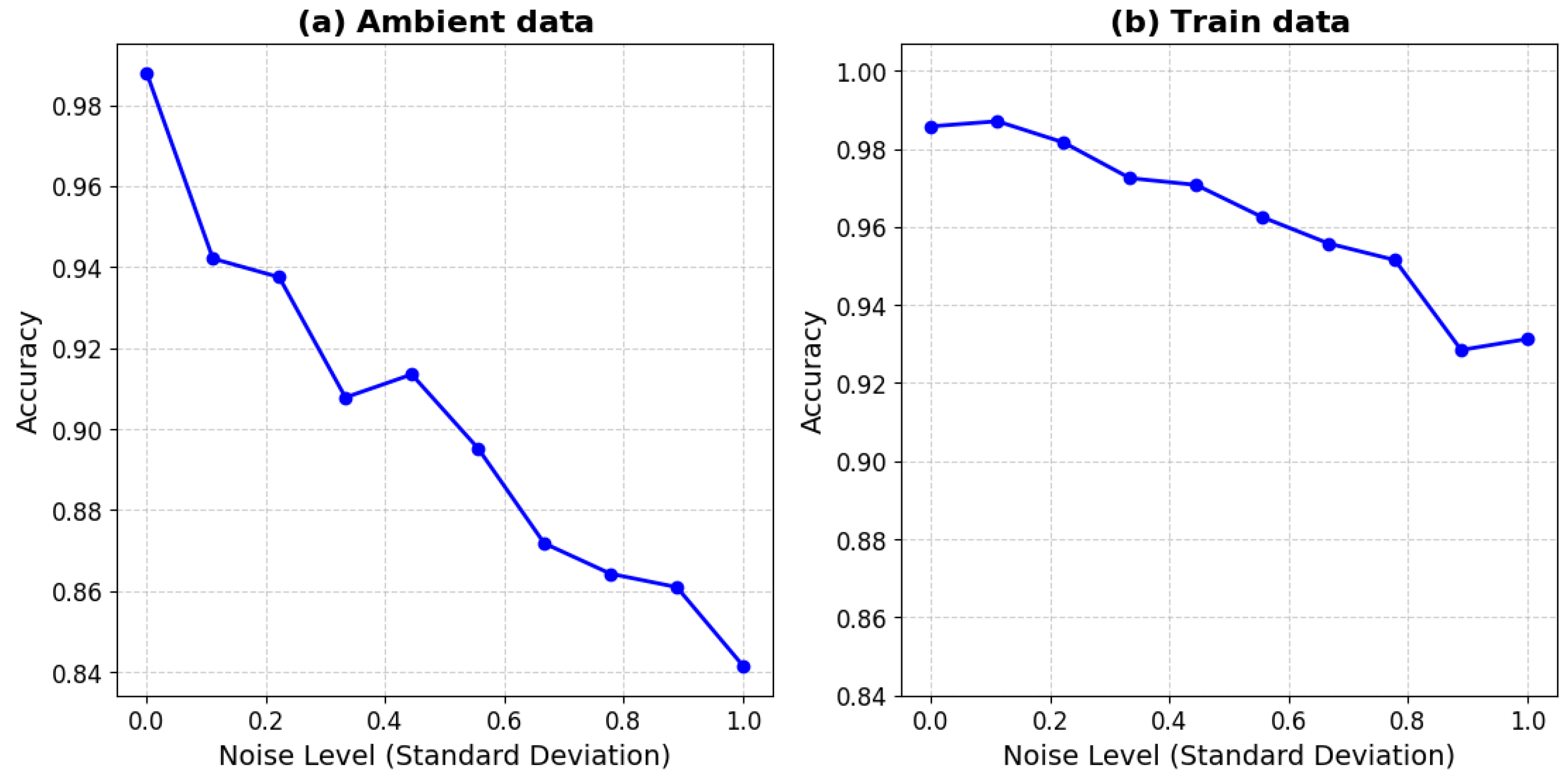
Figure 10.
Learning curves: training and validation accuracy.
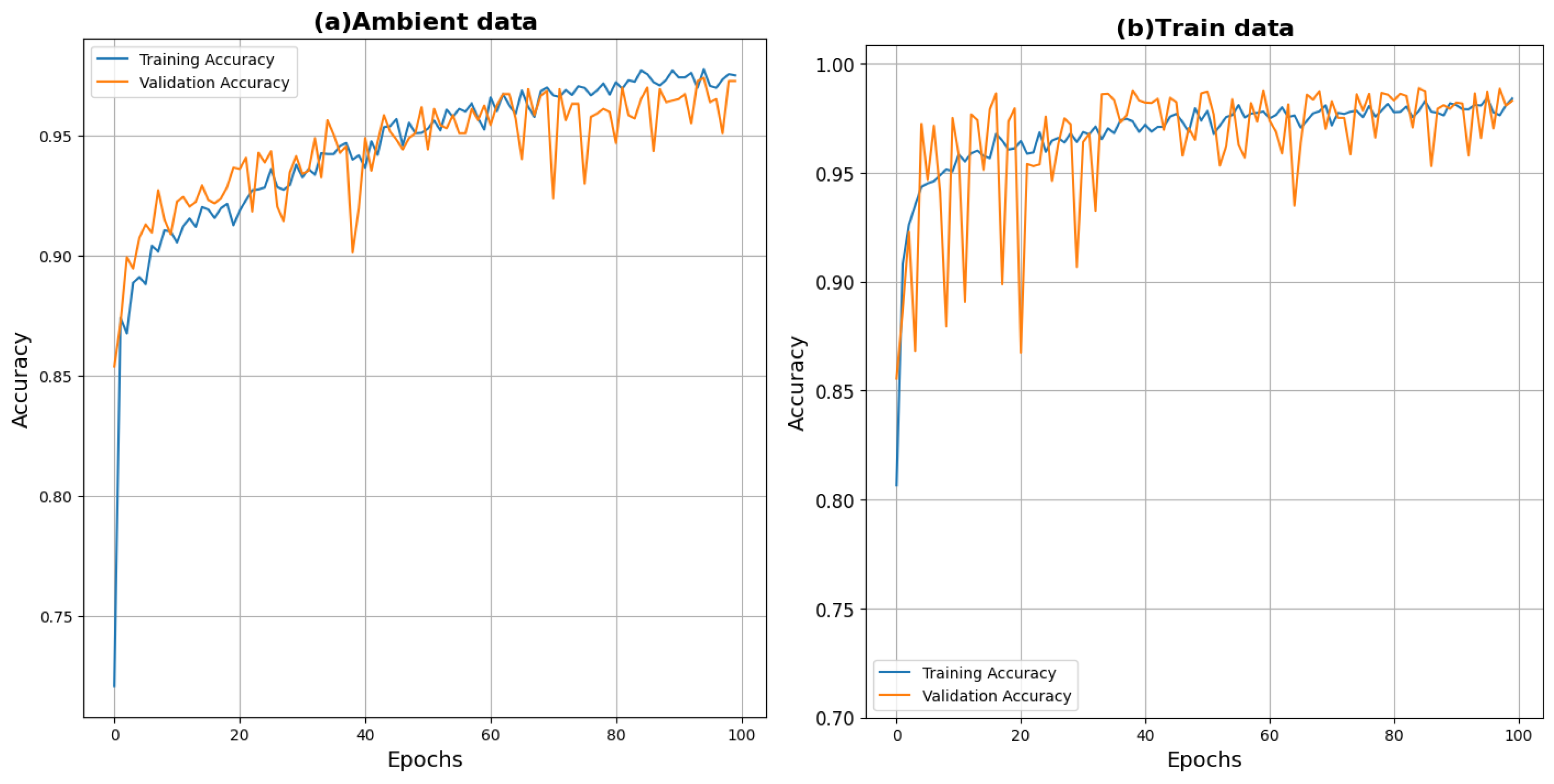

Table 1.
Cross-validation accuracy results for ambient and train data at 14 modal frequencies.
| Ambient Data | Train Data | ||
|---|---|---|---|
| Fold | Accuracy | Fold | Accuracy |
| Fold 1 | 0.7834 | Fold 1 | 0.7766 |
| Fold 2 | 0.7965 | Fold 2 | 0.7717 |
| Fold 3 | 0.8670 | Fold 3 | 0.7707 |
| Fold 4 | 0.8381 | Fold 4 | 0.7723 |
| Fold 5 | 0.8169 | Fold 5 | 0.7832 |
Table 2.
Cross-validation accuracy results for Ambient and Train data with the information of the evenly distributed 100 frequencies. The training and testing sizes are the same as the previous case.
Table 2.
Cross-validation accuracy results for Ambient and Train data with the information of the evenly distributed 100 frequencies. The training and testing sizes are the same as the previous case.
| Ambient Data | Train Data | ||
|---|---|---|---|
| Fold | Accuracy | Fold | Accuracy |
| Fold 1 | 0.9878 | Fold 1 | 0.9668 |
| Fold 2 | 0.9746 | Fold 2 | 0.9707 |
| Fold 3 | 0.9883 | Fold 3 | 0.9712 |
| Fold 4 | 0.9606 | Fold 4 | 0.9707 |
| Fold 5 | 0.9905 | Fold 5 | 0.9685 |
Disclaimer/Publisher’s Note: The statements, opinions and data contained in all publications are solely those of the individual author(s) and contributor(s) and not of MDPI and/or the editor(s). MDPI and/or the editor(s) disclaim responsibility for any injury to people or property resulting from any ideas, methods, instructions or products referred to in the content. |
© 2025 by the authors. Licensee MDPI, Basel, Switzerland. This article is an open access article distributed under the terms and conditions of the Creative Commons Attribution (CC BY) license (http://creativecommons.org/licenses/by/4.0/).
Copyright: This open access article is published under a Creative Commons CC BY 4.0 license, which permit the free download, distribution, and reuse, provided that the author and preprint are cited in any reuse.


