
Submitted:
28 June 2024
Posted:
02 July 2024
You are already at the latest version
Abstract
This paper investigates the integration of SHM within the frame of Industry 4.0 technologies, highlighting the potential for intelligent infrastructure management through the utilization of Big Data analytics, Machine Learning, and the Internet of Things (IoT). The study also presents a success case focused on a novel SHM methodology for detecting and locating damages in metallic aircraft structures, employing dimensional reduction techniques such as Principal Component Analysis (PCA). By analyzing strain data collected from a network of sensors and comparing it to a baseline pristine condition, the methodology aims to identify subtle changes in local strain distribution indicative of damage. Through extensive Finite Element Analysis (FEA) simulations and a PCA contribution analysis, the research explores the influence of various factors on damage detection, including sensor placement, noise levels, and damage size and type. The findings demonstrate the effectiveness of the proposed methodology in detecting cracks and holes as small as 2mm in length, showcasing the potential for early damage identification and targeted interventions in diverse sectors such as aerospace, civil engineering, and manufacturing. Ultimately, this paper underscores the synergistic relationship between SHM and Industry 4.0, paving the way for a future of intelligent, resilient, and sustainable infrastructure.
Keywords:
Industry 4.0
; Structural Health Monitoring
; damage detection and localization
; Machine learning
; Artificial intelligence
1. Introduction
Technology advancements are continuously improving our daily lives in all matters, from agriculture to astrophysics, with the proliferation of digital technologies such as artificial intelligence, big data analytics, the Internet of Things (IoT), additive manufacturing, and advanced robotics [1]. The possibilities for improvement are endless: products can be customized on demand, supply chains optimized as quickly as possible, and productivity reaches unprecedented levels. While Industry 4.0 comes with challenges like cybersecurity risks and workforce displacement, many see it as the gateway to a more agile, efficient, and sustainable industrial future.
Structural Health Monitoring (SHM) is a well-known concept and practice [2,3,4]. Figure 1 shows the main techniques of SHM. It is useful not only to prevent damage but also to extend the lifespan of elements, avoiding costs in maintenance, repair, and grounded or inoperable structures. The concept of using machine assistance for monitoring will lead to the next step of implementation of this methodology, with the continuous monitoring of elements.
SHM has become a topic of interest due to the large number of benefits it may provide to several industries, including reliability improvement and real-time damage detection, leading to lighter structures and maintenance cost reductions [5]. By implementing a real-time damage detection strategy, safety factors can be reduced under the damage-tolerant philosophy, especially for structures with high uncertainty in their failure modes (e.g., structures made of composite materials) [6].
One crucial aspect of SHM is the generation of vast amounts of data from sensors embedded in structures [7]. Machine learning and AI algorithms can analyze these data to extract valuable insights, patterns, and trends that may not be apparent through traditional methods. This analytical capability enables the identification of subtle changes in structural behavior over time, providing early warnings of potential issues.
Machine learning and AI techniques are particularly valuable in damage detection and classification [8]. By training models on labeled datasets, the system can learn to recognize specific damage signatures and distinguish them from normal operating conditions. This ability to detect and classify various types of damage, such as cracks, corrosion, or material degradation, contributes to effective and targeted maintenance efforts, where a human could take time with the large amount of data to process or be subject to human error caused by fatigue or inexperience.
With the advent of Fiber Optic Sensors (FOS), several SHM methodologies based on these sensors have been proposed in the scientific literature, being a suitable option for SHM of aerospace vehicles due to their small size, lightweight, and electromagnetic immunity, and multiplexing capability [9]. FOS are usually classified into local or point sensors (e.g. extrinsic Fabry-Perot interferometer), multi-point sensors (e.g. Fiber Bragg Gratings) and distributed sensors (e.g. Rayleigh and Brillouin distributed sensors) [10].
The future of SHM within Industry 4.0 is indeed bright. As these technologies continue to evolve and become more sophisticated, we can expect even more innovative applications that will shape the way we monitor, maintain, and ultimately safeguard our infrastructure for generations to come. This powerful combination has the potential to create a world where infrastructure is not just static and reactive, but rather intelligent, adaptable, and capable of anticipating and responding to the ever-changing demands of the modern world.
This paper delves into this by exploring how SHM will be propelled into a future of intelligent infrastructure management. Fed by the vast reserves of data collected from a dense network of sensors, advanced analytics will allow SHM systems to transition from just collecting data to predicting failure systems. Here, machine learning algorithms will sift through the vast amount of data, identifying patterns and anomalies that might signal potential problems.
This will enable targeted interventions before problems snowball into critical failures, saving time, money, and, most importantly, lives. Seamless communication strengthened by the Internet of Things will transform SHM systems into interconnected nodes within a larger industrial ecosystem. Traffic management systems can reroute vehicles to avoid overloading a bridge, while engineers are notified and can begin planning repairs.
This real-time exchange of information across various disciplines ensures a swift and coordinated response to potential threats, minimizing downtime and safeguarding public safety. Using the power of Industry 4.0, SHM promises to usher in a new era of proactive maintenance, improved safety, and optimized resource allocation, thus ensuring the longevity and resilience of infrastructures.
2. SHM Context within the Framework of Industry 4.0.
SHM transcends its traditional domain, evolving into a versatile technique for safeguarding infrastructures. For example in a bridge structure [11], its steel beams are instrumented with strain gauges and accelerometers and those sensors extract a lot of data, revealing early fatigue damage before it manifests as catastrophic failure. SHM extends the bridge’s lifespan, ensuring the safe passage of individuals and vehicles of all kinds [12].
Shifting focus to wind turbines, their blades transform kinetic energy from the wind into electrical energy, fiber optic sensors embedded within whispering tales of minute deflections [13]. These whispers unveil impending cracks under extreme weather, enabling timely interventions that optimize energy production while safeguarding these colossal structures.
In subterranean, aging pipelines [14] silently transport very important fluids and gases, mostly oil based fluids. Here, acoustic emission sensors act as vigilant guards, listening intently for leaks or the initiation of corrosion. Their timely warnings prevent environmental catastrophes and economic losses, ensuring the smooth flow of resources that humanity relies on [15].
SHM arises within the aerospace industry where aircraft wings, not just instruments of lift, but also embedded with a network of sensors could be monitoring about stress and potential damage during flight, making improvements in safety and operational efficiency, allowing to explore the skies with greater confidence [16].
SHM stands to be a game-changer within the Industry 4.0 paradigm, where intelligent machines and data-driven decisions. Sensors embedded within machinery and equipment constantly monitor their health, feeding a continuous stream of real-time data. Advanced analytics powered by machine learning algorithms can then analyze this data, not just detecting current problems but predicting equipment failure before it causes production issues. This proactive approach allows for preventative maintenance, minimizing downtime and optimizing production schedules.
SHM in Industry 4.0 lies in its ability to seamlessly integrate with other industrial processes, for example, an SHM system detecting a potential issue with a bridge could trigger a cascade of automated responses. Traffic management systems could reroute vehicles, while factories in the vicinity could adjust production schedules to minimize disruptions. This real-time communication across various industrial systems fosters an interconnected ecosystem, optimizing efficiency, safety, and cost-effectiveness. SHM data can be integrated with digital twin simulations, allowing engineers to virtually test potential repair scenarios and predict the effectiveness of interventions before physically implementing them. This not only streamlines maintenance processes but also minimizes risks and ensures the continued smooth operation of the entire industrial ecosystem.
SMH implementation in aerospace industry is a key factor to ensure high quality of spaceships and their parts in different stages like manufacturing and operation of parts and machines, the use of this technique is often classified as a non destructive test (NDT) and there are two main classes of measurement, the dynamic testing and static testing. Typically dynamic tests are related to measurement electrical and mechanical impedance and thermal measurements [17,18,19]; on the other hand, static tests regards electrical impedance and strain-based measurements [20,21].
The strain-based measurements are the ones that approached to the aerospace industry due to the effectiveness in damage detection [17], this does not mean it is easy to measure damage in structures, instead this method represents many challenges to measure small strain and also temperature changes. In order to partially overcome that challenges, a new approach is used by means of optical fiber sensors like fiber Bragg grating (FBG) [22,23]
SHM techniques are developing constantly in order to enhance damage detection increasingly smaller in size and also reducing false indications. There are another approaches in SMH with piezo-electric and piezo-resistive sensors in which the materials induces an electric charge when its shape changes due to stresses, but not often used in aerospace industry since they are heavy, susceptible to failure under greater strains and their size could result in installation issues [16], however, piezo-electric sensors are cheaper to acquire.
SHM is primordial in modern manufacturing processes, particularly within Industry 4.0. Its application has so many nuances in manufacturing, varying from monitoring the health of manufacturing equipment and facilities to ensuring the integrity of the products themselves [24,25,26]. In this context, SHM systems are employed to continuously assess the structural integrity of critical components and machinery, detecting any deviations from normal operating conditions.
By utilizing a network of sensors and advanced data analytics, SHM can provide real-time insights into equipment performance, alerting operators to potential failures or inefficiencies before they occur [27,28]. This proactive approach to maintenance enhances operational efficiency, reduces downtime, and ensures the safety and reliability of manufacturing processes [29,30]. Furthermore, SHM enables predictive maintenance [31], optimizing maintenance schedules based on actual equipment condition rather than predefined intervals, resulting in cost savings and improved asset utilization. As Industry 4.0 continues to evolve, the integration of SHM into manufacturing processes [32] will be essential, so that efficiency, productivity, and product quality could be higher.
Embedded sensors, strategically placed on critical equipment and machinery, continuously monitor parameters like vibration [33], strain [34], and temperature [35]. This data stream feeds into real-time analytics, allowing for the detection of anomalies and potential equipment degradation before they escalate into catastrophic failures. This empowers predictive maintenance, enabling targeted interventions at the early stages of wear and tear, minimizing time where the part o machine are inoperative and maximizing production efficiency [36,37,38].
Additionally, SHM data can be integrated with digital twin technology [39], creating virtual simulations of equipment performance, which can be used to optimize maintenance schedules and predict the impact of future operational changes, ultimately leading to enhanced process control and cost reduction in the manufacturing environment.
SHM revolutionizes this approach by integrating sensors, data acquisition systems, and advanced analytics. These systems continuously monitor structural behavior, collect data regarding to loads, vibrations, temperature, and other environmental factors, and provide real-time insights. By doing it, SHM enables early detection of defects, fatigue and anomalies, allowing for timely maintenance and preventing catastrophic failures.
Artificial Intelligence (AI) offers significant potential to enhance SHM by enabling the analysis of complex sensor data sets. Machine learning algorithms can be applied to identify fine patterns and anomalies that may be missed by conventional methods and this capability allows the early detection of damage significantly before it progresses to a critical stage [40,41].
Besides, AI can be trained on historical data to predict the degradation of a structure over time [42,43], facilitating a transition from reactive repairs to preventative maintenance strategies . This proactive approach not only reduces life-cycle costs but also minimizes the risk of catastrophic failures by addressing issues before they escalate and by integrating AI with SHM systems, infrastructure can be transformed into intelligent entities capable of communicating their health status and anticipating future maintenance needs [44,45,46].
SHM has entered the age of big data because of the network of sensors embedded in bridges, buildings, and other structures generates massive amounts of data on strain, vibration, and environmental conditions. This massive amount of data, while valuable, presents a challenge and traditional analysis methods struggle to keep pace with the sheer volume and complexity of the information.
Big data offers a solution by employing big data analytics, engineers can unlock the hidden insights within the SHM data [47], so these techniques allow for real-time monitoring, enabling early detection of potential problems before they become critical. The introduction of Big data in SHM has improved the data managements in terms of collecting, storing and analyzing massive amounts of data with real-time processing [48,49], so adding machine learning to Big data results in predictions about patterns and anomalies that might indicate structural damage and the insights from the data analysis can be used to predict potential failures, so the lifespan of the structure could be increase and then catastrophic failures are prevented [50,51].
Big data facilitates the identification of patterns and trends that can predict future issues, allowing for preventive maintenance strategies. This change from reactive repairs to proactive interventions extends the lifespan of structures, reduces costs, and ultimately enhances public safety. Therefore, big data makes SHM from a simple monitoring system into a powerful predictive tool.
SHM is facing towards big steps in sensor integration, internet of things and advance data analytics in order to improve the performance when making decisions about structural damage. sensor integration and miniaturization are about devices that are more embedded within the very fabric of structures, this would take into account more comprehensive and continuous monitoring, providing a more global view of a structure’s health [52]. Additionally, miniaturized sensors would be less intrusive and easier to deploy on existing infrastructure.
The internet of things and cloud computing are another future trends in an era of interconnected SHM systems, since, sensors embedded in bridges, buildings, and other structures will constantly transmit real-time data to a central cloud platform [53]. This facilitates remote monitoring and centralized analysis by experts, who can diagnose issues from anywhere in the world and cloud computing also offers virtually limitless storage and processing power, making it easier to handle the ever growing data stack from SHM systems, so the scalability of cloud-based SHM systems will allow easy integration of additional sensors and data sources in the future and getting ready for even more comprehensive structural health assessments [54,55,56].
Another trend is related to data analytics and here, machine learning algorithms will become even more sophisticated and capable of not only identifying damage but also predicting its future progression and recommending optimal maintenance strategies [57]. This information can be used to create digital twins or virtual replicas of real world structures and these can be continually updated with real-time sensor data, allowing engineers to virtually test different repair scenarios and predict the effectiveness of various interventions [58,59].
3. Materials and Methods
With the evolution of computer sciences, the improvement of the hardware through time and apparition of new software that allows the quick and easy implementation of machine learning code, the substitution of a human constant monitoring has been decreasing and the use of new tools of the Industry 4.0 and Artificial Intelligence is now increasing for the prevention of structural damage. The base of theses tools are the basics algorithms and schemes of machine learning, who can be seen in Figure 2. The combination of these data process methods, with the different SHM monitoring system consist in the next step of maintenance, and are used in civil, mechanical engineering, transports and all sort of structural domain.
3.1. Descriptive Methods
Descriptive methods in machine learning involve analyzing and summarizing data to gain insights into its patterns and characteristics. These methods focus on understanding the inherent structure of the data rather than making predictions [61]. Descriptive techniques include statistical measures, visualization tools, and clustering algorithms that help reveal trends, distributions, and relationships within the dataset. By providing a comprehensive overview of the data, descriptive methods serve as a crucial initial step in the machine learning process, guiding subsequent modeling decisions and ensuring a solid foundation for further analysis. These techniques are often called unsupervised methods; they don’t need a labeled dataset and are capable to recognize a behavior in the characteristics. The data set and model will have the next characteristics:
- Recent historical data: The dataset is the basement of this analysis, and the model search a tendency in recent behavior or events, if the dataset provides older historical data, the model will not be able to simulate and classify the recent events, that’s why it’s needed to be purged to only have recent data that are in accord with the modern tendency.
- Nonexistence of an objective variable: as said before, these models focus in the inherent structure rather than making prediction. The model will search the best way to describe a phenomenon rather than maximize or predict a numerical value.
Clustering, exemplified by the k-means technique, is a method in machine learning that groups similar data points together based on shared characteristics. K-means iteratively partitions the dataset into k clusters, with each cluster represented by its centroid. This approach is widely used for segmentation and pattern recognition, enabling the identification of distinct subgroups within a larger dataset.
Factor selection involves choosing relevant variables to improve model performance. Regression trees utilize a tree-like structure to recursively split data based on variables, identifying key predictors for the target variable. On the other hand, Principal Component Analysis (PCA) is a dimensionality reduction technique that transforms the original variables into a smaller set of uncorrelated components. Both regression trees and PCA contribute to factor selection by emphasizing the most influential variables, aiding in the creation of more efficient and interpretable models.
3.2. Predictive Methods
Predictive methods in machine learning involve leveraging algorithms to analyze historical data and identify patterns, enabling the model to make predictions or classifications for new, unseen data. These methods use mathematical models to learn relationships between input features and output labels, adjusting their parameters through training processes. Common predictive techniques include regression for continuous outcomes and classification for discrete categories. The goal is to create a model that generalizes well to unseen data, providing accurate predictions and insights based on the patterns it has learned during training. These techniques are often called supervised methods; they need a labeled dataset to train and recognize the results in a large but closed options. The data set and model will have the next characteristics:
- Historical data: The dataset can be formed of older historical data compared to the descriptive methods. While it describe the same event, it doesn’t matter if the data came from 5 years or 20 years ago. The dataset has to be labeled with the expected results.
- Existence of an objective variable: In this case, the model has to predict a results, it can be numerical or no numerical, in which case it’s replace by a binary dummy.
- Relation between the predictive and results variables: The data set has to be cleaned and analyzed to select the variables which can be in direct relation with the objective variable, a condition that the descriptive method doesn’t need.
Classification involves assigning predefined labels to input data based on its features. Neural networks, comprising interconnected nodes organized in layers, are adept at learning complex patterns and relationships within data for accurate classification. Decision trees recursively split the dataset based on feature conditions, constructing a tree-like structure for efficient classification. Support Vector Machines (SVM) excel in finding optimal hyperplane to separate distinct classes in high-dimensional space, making them versatile for linear and non-linear classification tasks. K-Nearest Neighbors (KNN) classifies data points based on the majority class among their k-nearest neighbors, providing a straightforward yet effective approach. These diverse classification techniques cater to various data structures and problem complexities, showcasing the versatility of machine learning in solving real-world classification challenges across different domains.
Regression involves predicting continuous values based on input features. Neural networks excel by learning complex patterns for accurate predictions. Time series regression models temporal trends, suitable for time-dependent data. Support Vector Machines SVM for regression find optimal hyperplane to capture non-linear relationships in the data. These techniques, including neural networks, time series, and SVM, offer adaptable solutions for predicting numerical values across diverse domains.
3.3. Virtual Testing Setup
In order to perform a virtual testing methodology within the SHM context, a whole MQ1 predator aircraft wing structure made of aluminum alloy 2024-T3 was selected as a structural component for this study. This structure is composed of three beams, 18 ribs, and skins [62]. Rivets and other structural joints were replaced by perfect contacts between bodies and control surface mechanisms. Fuel tanks, and other systems were neglected to reduce computational cost. In Figure 3 the drawing views of the wing structure can be appreciated.
Static Structural Simulation solver in Ansys was used, neglecting non-linear effects. Boundary conditions for this model included a fixed support for each beam at the root and a distributed load over the lower skin accounting for the total generated lift for this aircraft at steady cruise flight condition; considering a weight of 766 kg giving an equivalent load of 3753 N for each semi-wing approximately.
The elements used on the model’s mesh were hexahedral using a multi-zone method overall beams and fine refinement in the main beam (which was the focus of the study) to avoid obtaining significant changes in the mesh when damages were defined, these damages can be observed in Figure 5. These were located at several positions as can be seen in Figure 4. Additionally, beams, ribs, and skin were modeled with shell elements to reduce the overall model complexity, obtaining a total number of 50144 elements with a minimum element quality of 0.22 (this index shows a mesh reliability criteria having maximum reliability at 1).
The main studied component for this structure was the leading edge beam (main beam) of the aircraft wing. 408 virtual strain sensors were defined along the beam, 102 sensors were located at the top face of the beam, 102 at the lower face, 102 at the front face, and 102 at the back face. These virtual sensors were configured to obtain the normal strains in the longitudinal axis of the beam, emulating FBGs sensors.
Mesh convergence was determined by comparing mesh degrees of freedom (DOF) with the wing’s maximum deflection, obtaining the trend shown in Figure 6 which shows a mesh convergence around 440000 DOF. This configuration was achieved with a general element size of 15 mm along the geometry and a special refinement of 5 mm near damages.
However, since in this experiment strain field around very small damages (compared with the structure size) had to be analyzed, the biggest number of elements allowed with the computational capacity available was used, making a special mesh refinement around the damages.
Two damage types were analyzed, a circular hole and a high aspect ratio rhombus which simulates a crack. Three different damage sizes were defined for each damage type: 20 mm, 10 mm, and 2 mm diameter for holes and the length of the largest diagonal for rhombus (with an aspect ratio equal to 10). Three different locations were defined for damages: 25%, 50%, and 75% of wingspan. Table 1 shows damage locations and sizes.
To emulate a real sensing scheme by using FBGs, different experimental trials were artificially defined. The trials were based on the strains measured for each sensor and replicated I times using a random number based on a Gaussian distribution, with a mean equal to the initial strain value and a standard deviation equal to . This deviation was chosen considering that the sensitivity of today’s available FBGs sensing techniques is near to . In this way, dimensions for each data matrix were 1000 × 600 for baseline , 700 × 600 for validation data and 900 × 600 for damages ( to ).
Several sensitivity analyses were performed which included, how changes score as a function of the number of operative sensors. By performing the detection algorithm several times and removing artificially some sensors each time, the change of score with respect to the variation of artificial noise was evaluated.
To validate the model, an experiment based on a double supported steel beam was replicated performing a cross-validation with Ansys [50]. For this model, two fixed supports were defined at both ends of the beam and a vertical load at the middle as shown in Figure 7, also all geometry was meshed with 2 mm shell elements. In this validation, the variable to evaluate convergence was the maximum bending moment. Several loads were applied and compared with the minimum safety factor associated with each load, finally, a linear regression was performed and the load corresponding to a safety factor equal to one was determined.
3.4. Damage Detection Methodology
For the experiments presented in this work (simulations of the damaged structure by cracks and holes with their respective variations), each data set was organized into a matrix , where I is the trial number and J the sensor number. As mentioned before, the main objective of PCA is to reduce J to several principal components retaining a representative amount of total variability (90% was selected for this study which was obtained by retaining three principal components) according to Jolliffe [63].
To achieve this, matrix, that corresponds to covariance eigenvalues of A, was calculated for data set, whilst remaining data sets (for damage conditions) are projected using P matrix calculated for BL. Principal component matrix T is given by equation (1) where the first three columns of T correspond to the three first principal components of new data set [64].
In a subsequent step Q statistic is calculated. Initially the residual error matrix E is calculated according to equation (3), is calculated as shown in equation (2)
With these values Q statistic array is calculated as shown in equation (4) where denotes row of E matrix.
After that is calculated as shown in equation (5), being the row of A matrix and being a diagonal matrix composed by eigenvalues of A.
To determine if there is a damage or not, a "damage threshold" is defined based on BL’s inverse distribution. To calculate this threshold , mean and variance of Q and for BL data set is calculated by means of equations (6) and (7) [65]:
Being squared inverse statistical distribution for a given confidence level , previous experiments reported by Sierra et al showed that using alpha values between 95% and 99% give accepted results [66]. It is important to mention that D0 correspond to a validation data set (pristine state) and, in this sense, statistics for D0 should be located under threshold while data for damaged conditions should be located over the threshold.
According to the threshold each datum is classified as true when data is over the threshold and false when data is under the threshold being true data considered as detected damage. Having this into account ROC analysis was carried out, classifying data as true positive (), true negative(), false positive () and false negative () as mentioned before. Finally, score which determines experiment accuracy was calculated according to equation (8), this score (taking values between 0 and 1) is a measure of data classification accuracy and in terms of SHM methodology a higher value of this score is a meaning of a damage detected successfully.
3.5. Damage Localization Methodology
Once Q and statistics were calculated (and having a data set with a damage detected successfully) contribution analysis is performed, this analysis assigns a numerical value to each column (or data measured by each sensor) of the original data set which quantifies the influence of each row to the increase of Q and statistics, in terms of SHM methodology damage is located to sensors (or rows of the original data set) with a higher contribution magnitude. Contribution analysis for Q statistic is calculated according to equation (9).
Where is row of identity matrix and contains contribution of each row based on Q statistic. Similar Q statistic contribution analysis is given by the equation 10.
Once having contribution values for each sensors damage localization is estimated based on the sensors with the most quantity of contribution.
4. Results and Discussion
After applying methodology purposed previously score based on Q statistic is obtained for each damage type and location, Table 2 and Table 3 shows obtained score values for crack a hole damages respectively. Additionally Figure 9 shows Q statistic distribution by each measurement and its location relative to defined threshold.
Once identifying an existent damage contribution analysis was performed, in this analysis most contributing sensors were defined according to Table 4 and Table 5:
In most cases contributing sensor was in the lower face of the beam and near to the actual damage, it should be note that in this application typically lower face is under maximum tensile stresses and strains. Additionally it is important to note that there are undetected damages in which most contributing sensor is result of system noise and not a product of damage locations, this because contribution analysis is only valid if a damage is detected, for this reason several contribution results are rejected.
Figure 10 and Figure 11 shows a representative heat map with the contribution level around the beam for different damages. In these maps damage location is clearly identified when score level is high, otherwise highest contribution is not clearly marked in one concentrated spot.
In the sensitivity analysis based on operative number of sensors one of the biggest damages (20 mm length at 25%) was chosen for performing previous calculations removing one by one nearest sensors to the damage at each iteration obtaining trends shown in Figure 12, based on given results is noted that 15 nearest sensors to the damage can be inoperative and damage can be detected normally for both damage types (hole and crack).
For the sensitivity analysis based in noise a detected damage on the prior results was chosen (10 mm length at 75%), with this damage score was calculated for several noise levels varying noise from to . As can be seen in Figure 13 with a noise of damage can be detected for both cases otherwise damage cannot be detected.
According to Table 4 and Table 5 damages with the lowest performance of the technique correspond to damages for hole and crack. These damages were analyzed at different noise levels to determine an adequate level for achieving acceptable score results.
As shown in Figure 14 it is possible to detect smaller damages as long as noise level be as low enough, compared with minimum noise in previous analysis this noise decreases at levels around
5. Conclusions
SHM is on the cusp of a revolutionary transformation as it merges with the core principles of Industry 4.0. This paper has explored the various areas where this synergy will have the most significant impact, fundamentally reshaping how we approach infrastructure management across diverse sectors.
Big data analytics and machine learning algorithms will unlock the hidden potential within the vast amount of SHM data. That amount of data will no longer be a mere record of the past, it will become a powerful tool for predicting future issues. This newly predictive power will extend the lifespan of structures in a variety of domains, from the delicate wings of an aircraft to buildings that support our cities. Early detection of anomalies will enable targeted interventions before problems escalate, leading to significant cost savings and improved safety across all fields.
Real-time communication will enable proactive responses to potential issues before they snowball into major disruptions. Data acquisition is then immediately transmitted to a central hub, triggering a cascade of automated responses to interconnected ecosystems, optimizing efficiency, safety, and cost-effectiveness in ways never before imagined.
Sensitivity of FBG’s is a key factor for detecting small damage, related to the strain field generated by the damage that is proportional to itself; if it is not high enough it will not be sensed. However, the strain field is related to stress concentrations, and these concentrations depend on geometry and size. For this, damage type is important too, because each damage type has a different geometry and therefore a different stress concentration.
In this article, several sensitivity analyzes were performed, resulting in the conclusion that sensor noise and the number of sensors are key factors to have adequate accuracy in this methodology. This study is based on FBG’s available nowadays, however, sensitivity analysis results presented in this analysis show the improvement in the methodology if FBG’s performance is improved and how, with SHM accuracy, it can overcome traditional NDT techniques.
However, FBG locations play an important role in damage detection; They have to be located at the points where the strains are highest and near possible damages; otherwise, they will sense noise or very low strain fields. For this reason, there are sensors near to damages that are not enough contributing to statistical indexes, although they are near to the damage.
The main advantage of strain-based SHM with respect to other SHM techniques is sensitivity for damage detection. With this technique, damages of 2 mm length can be easily detected, while in other techniques the minimum damage length has to be 10 times bigger. This is important in applications where dynamic loads are prevalent, because if damage can be detected early in its growth, it will give an extended response time to take corrective action.
The future of SHM within Industry 4.0 is promising. As these technologies continue to evolve and become more sophisticated, more innovative applications that will reshape how we monitor, maintain, and ultimately safeguard our infrastructure will appear. This powerful combination has the potential to create a world where infrastructure is not just static and dynamic, but intelligent, adaptable, and capable of anticipating and responding to the changing demands of the modern world.
Author Contributions
Conceptualization, A.R.H., J.A., C.H., S.R., R.E.V., and J.S.P.; methodology, A.R.H., J.A., and J.S.P.; validation, J.R., J.S.P., and R.E.V.; formal analysis, A.R.H., J.A., C.H., S.R., R.E.V., C.A.E., and J.S.P.; investigation, A.R.H., J.A., C.H., S.V., and J.S.P.; writing—original draft preparation, A.R.H., J.A., C.H., S.R., and C.A.E.; writing—review and editing, J.S.P., and R.E.V.; supervision, J.R., J.S.P., and R.E.V. All authors have read and agreed to the published version of the manuscript.
Funding
This work was developed with the funding of the Universidad Pontificia Bolivariana (UPB) and with the support of the Universidad Nacional de Colombia in association with Contraloría General de la República in the frame of Contract CGR-373-2023.
Institutional Review Board Statement
Not applicable.
Informed Consent Statement
Not applicable.
Acknowledgments
Not applicable.
Conflicts of Interest
The authors declare no conflict of interest.
References
- Cárdenas-Robledo, L.A.; Hernández-Uribe, O.; Reta, C.; Cantoral-Ceballos, J.A. Extended reality applications in industry 4.0. – A systematic literature review. Telematics and Informatics 2022, 73, 101863. [Google Scholar] [CrossRef]
- Mishra, M. Machine learning techniques for structural health monitoring of heritage buildings: A state-of-the-art review and case studies. Journal of Cultural Heritage 2021, 47, 227–245. [Google Scholar] [CrossRef]
- Ahmed, O.; Wang, X.; Tran, M.V.; Ismadi, M.Z. Advancements in fiber-reinforced polymer composite materials damage detection methods: Towards achieving energy-efficient SHM systems. Composites Part B: Engineering 2021, 223, 109136. [Google Scholar] [CrossRef]
- Zaparoli Cunha, B.; Droz, C.; Zine, A.M.; Foulard, S.; Ichchou, M. A review of machine learning methods applied to structural dynamics and vibroacoustic. Mechanical Systems and Signal Processing 2023, 200, 110535. [Google Scholar] [CrossRef]
- Farrar, C.R.; Worden, K. An introduction to structural health monitoring. Philosophical Transactions of the Royal Society A: Mathematical, Physical and Engineering Sciences 2007, 365, 303–315. [Google Scholar] [CrossRef] [PubMed]
- Abouzeida, E.; Quinones, V.; Gowayed, Y.; Soobramaney, P.; Flowers, G.; Black, R.J.; Costa, J.M.; Faridian, F.; Moslehi, B. Design, manufacture and testing of an FBG-instrumented composite wing. AIP Conference Proceedings;, 2014; Vol. 1581 33, pp. 1141–1148. [CrossRef]
- Han, J. Data mining, ed., 3rd ed.; Morgan Kaufmann series in data management systems; Morgan Kaufmann/Elsevier: Waltham, MA, 2012. [Google Scholar]
- Khazaee, M.; Derian, P.; Mouraud, A. A comprehensive study on Structural Health Monitoring (SHM) of wind turbine blades by instrumenting tower using machine learning methods. Renewable Energy 2022, 199, 1568–1579. [Google Scholar] [CrossRef]
- Glisic, B.; Inaudi, D. Fibre Optic Methods for Structural Health Monitoring; John Wiley & Sons: Chichester, UK, 2007. [Google Scholar]
- Güemes, A.; Fernandez-Lopez, A.; García-Ramírez, J.; Reyes-Perez, M.E.; Zurita, F.C. Simulation Tools for a Fiber-Optic Based Structural Health Monitoring System. Transactions of Nanjing University of Aeronautics and Astronautics 2018, 35, 219–225. [Google Scholar] [CrossRef]
- Worden, K.; Cross, E. On switching response surface models, with applications to the structural health monitoring of bridges. Mechanical Systems and Signal Processing 2018, 98, 139–156. [Google Scholar] [CrossRef]
- An, Y.; Chatzi, E.; Sim, S.; Laflamme, S.; Blachowski, B.; Ou, J. Recent progress and future trends on damage identification methods for bridge structures. Structural Control and Health Monitoring 2019, 26. [Google Scholar] [CrossRef]
- Liu, Z.; Zhang, L. A review of failure modes, condition monitoring and fault diagnosis methods for large-scale wind turbine bearings. Measurement 2020, 149, 107002. [Google Scholar] [CrossRef]
- Wright, R.F.; Lu, P.; Devkota, J.; Lu, F.; Ziomek-Moroz, M.; Ohodnicki, P.R. Corrosion Sensors for Structural Health Monitoring of Oil and Natural Gas Infrastructure: A Review. Sensors 2019, 19, 3964. [Google Scholar] [CrossRef] [PubMed]
- Ho, M.; El-Borgi, S.; Patil, D.; Song, G. Inspection and monitoring systems subsea pipelines: A review paper. Structural Health Monitoring 2019, 19, 606–645. [Google Scholar] [CrossRef]
- Rocha, H.; Semprimoschnig, C.; Nunes, J.P. Sensors for process and structural health monitoring of aerospace composites: A review. Engineering Structures 2021, 237, 112231. [Google Scholar] [CrossRef]
- Giurgiutiu, V.; Zagrai, A. Damage Detection in Thin Plates and Aerospace Structures with the Electro-Mechanical Impedance Method. Structural Health Monitoring 2005, 4, 99–118. [Google Scholar] [CrossRef]
- Winklberger, M.; Kralovec, C.; Humer, C.; Heftberger, P.; Schagerl, M. Crack Identification in Necked Double Shear Lugs by Means of the Electro-Mechanical Impedance Method. Sensors 2020, 21, 44. [Google Scholar] [CrossRef]
- Bergmayr, T.; Kralovec, C.; Schagerl, M. Vibration-Based Thermal Health Monitoring for Face Layer Debonding Detection in Aerospace Sandwich Structures. Applied Sciences 2020, 11, 211. [Google Scholar] [CrossRef]
- Güemes, A.; Fernandez-Lopez, A.; Pozo, A.R.; Sierra-Pérez, J. Structural Health Monitoring for Advanced Composite Structures: A Review. Journal of Composites Science 2020, 4, 13. [Google Scholar] [CrossRef]
- Hunt, S.R.; Hebden, I.G. Validation of the Eurofighter Typhoon structural health and usage monitoring system. Smart Materials and Structures 2001, 10, 497–503. [Google Scholar] [CrossRef]
- Zhang, H.; Liu, T.; Lu, J.; Lin, R.; Chen, C.; He, Z.; Cui, S.; Liu, Z.; Wang, X.; Liu, B.; Xiong, K.; Wu, Q. Static and ultrasonic structural health monitoring of full-size aerospace multi-function capsule using FBG strain arrays and PSFBG acoustic emission sensors. Optical Fiber Technology 2023, 78, 103316. [Google Scholar] [CrossRef]
- Chen, C.; Wu, Q.; Xiong, K.; Zhai, H.; Yoshikawa, N.; Wang, R. Hybrid Temperature and Stress Monitoring of Woven Fabric Thermoplastic Composite Using Fiber Bragg Grating Based Sensing Technique. Sensors 2020, 20, 3081. [Google Scholar] [CrossRef]
- Gardner, L. Metal additive manufacturing in structural engineering – review, advances, opportunities and outlook. Structures 2023, 47, 2178–2193. [Google Scholar] [CrossRef]
- Segura, P.; Lobato-Calleros, O.; Ramírez-Serrano, A.; Soria, I. Human-robot collaborative systems: Structural components for current manufacturing applications. Advances in Industrial and Manufacturing Engineering 2021, 3, 100060. [Google Scholar] [CrossRef]
- Tian, Y.; Chen, C.; Sagoe-Crentsil, K.; Zhang, J.; Duan, W. Intelligent robotic systems for structural health monitoring: Applications and future trends. Automation in Construction 2022, 139, 104273. [Google Scholar] [CrossRef]
- Gordan, M.; Sabbagh-Yazdi, S.R.; Ismail, Z.; Ghaedi, K.; Carroll, P.; McCrum, D.; Samali, B. State-of-the-art review on advancements of data mining in structural health monitoring. Measurement 2022, 193, 110939. [Google Scholar] [CrossRef]
- Maes, K.; Van Meerbeeck, L.; Reynders, E.; Lombaert, G. Validation of vibration-based structural health monitoring on retrofitted railway bridge KW51. Mechanical Systems and Signal Processing 2022, 165, 108380. [Google Scholar] [CrossRef]
- Chadha, M.; Ramancha, M.K.; Vega, M.A.; Conte, J.P.; Todd, M.D. The modeling of risk perception in the use of structural health monitoring information for optimal maintenance decisions. Reliability Engineering &; System Safety 2023, 229, 108845. [Google Scholar] [CrossRef]
- Orcesi, A.D.; Frangopol, D.M. Optimization of bridge maintenance strategies based on structural health monitoring information. Structural Safety 2011, 33, 26–41. [Google Scholar] [CrossRef]
- Ndinga Okina, S.; Taillandier, F.; Ahouet, L.; Hoang, Q.A.; Breysse, D.; Louzolo-Kimbembe, P. Using Conceptual Graph modeling and inference to support the assessment and monitoring of bridge structural health. Engineering Applications of Artificial Intelligence 2023, 125, 106665. [Google Scholar] [CrossRef]
- Ghosh, A.; Edwards, D.J.; Hosseini, M.R.; Al-Ameri, R.; Abawajy, J.; Thwala, W.D. Real-time structural health monitoring for concrete beams: a cost-effective ‘Industry 4.0’ solution using piezo sensors. International Journal of Building Pathology and Adaptation 2020, 39, 283–311. [Google Scholar] [CrossRef]
- Goyal, D.; Pabla, B.S. The Vibration Monitoring Methods and Signal Processing Techniques for Structural Health Monitoring: A Review. Archives of Computational Methods in Engineering 2015, 23, 585–594. [Google Scholar] [CrossRef]
- Katsikeros, C.; Labeas, G. Development and validation of a strain-based Structural Health Monitoring system. Mechanical Systems and Signal Processing 2009, 23, 372–383. [Google Scholar] [CrossRef]
- Dutta, C.; Kumar, J.; Das, T.K.; Sagar, S.P. Recent Advancements in the Development of Sensors for the Structural Health Monitoring (SHM) at High-Temperature Environment: A Review. IEEE Sensors Journal 2021, 21, 15904–15916. [Google Scholar] [CrossRef]
- Fu, T.S.; Ghosh, A.; Johnson, E.A.; Krishnamachari, B. Energy-efficient deployment strategies in structural health monitoring using wireless sensor networks: ENERGY-EFFICIENT DEPLOYMENT USING WIRELESS SENSOR NETWORKS. Structural Control and Health Monitoring 2012, 20, 971–986. [Google Scholar] [CrossRef]
- Dong, T.; Haftka, R.T.; Kim, N.H. , Advantages of Condition-Based Maintenance over Scheduled Maintenance Using Structural Health Monitoring System. In Reliability and Maintenance - An Overview of Cases; IntechOpen, 2019; pp. 11–36. [CrossRef]
- Gunawan, F.E.; Nhan, T.H.; Asrol, M.; Kanto, Y.; Kamil, I.; Sutikno. A New Damage Index for Structural Health Monitoring: A Comparison of Time and Frequency Domains. Procedia Computer Science 2021, 179, 930–935. [Google Scholar] [CrossRef]
- Honghong, S.; Gang, Y.; Haijiang, L.; Tian, Z.; Annan, J. Digital twin enhanced BIM to shape full life cycle digital transformation for bridge engineering. Automation in Construction 2023, 147, 104736. [Google Scholar] [CrossRef]
- Azimi, M.; Eslamlou, A.; Pekcan, G. Data-Driven Structural Health Monitoring and Damage Detection through Deep Learning: State-of-the-Art Review. Sensors 2020, 20, 2778. [Google Scholar] [CrossRef] [PubMed]
- Sun, L.; Shang, Z.; Xia, Y.; Bhowmick, S.; Nagarajaiah, S. Review of Bridge Structural Health Monitoring Aided by Big Data and Artificial Intelligence: From Condition Assessment to Damage Detection. Journal of Structural Engineering 2020, 146. [Google Scholar] [CrossRef]
- Flah, M.; Nunez, I.; Ben Chaabene, W.; Nehdi, M.L. Machine Learning Algorithms in Civil Structural Health Monitoring: A Systematic Review. Archives of Computational Methods in Engineering 2020, 28, 2621–2643. [Google Scholar] [CrossRef]
- Yuan, F.G.; Zargar, S.A.; Chen, Q.; Wang, S. Machine learning for structural health monitoring: challenges and opportunities. Sensors and Smart Structures Technologies for Civil, Mechanical, and Aerospace Systems 2020; Zonta, D.; Sohn, H.; Huang, H., Eds. SPIE, 2020. [CrossRef]
- Salehi, H.; Burgueño, R. Emerging artificial intelligence methods in structural engineering. Engineering Structures 2018, 171, 170–189. [Google Scholar] [CrossRef]
- Malekloo, A.; Ozer, E.; AlHamaydeh, M.; Girolami, M. Machine learning and structural health monitoring overview with emerging technology and high-dimensional data source highlights. Structural Health Monitoring 2021, 21, 1906–1955. [Google Scholar] [CrossRef]
- Vagnoli, M.; Remenyte-Prescott, R.; Andrews, J. Railway bridge structural health monitoring and fault detection: State-of-the-art methods and future challenges. Structural Health Monitoring 2017, 17, 971–1007. [Google Scholar] [CrossRef]
- Entezami, A.; Sarmadi, H.; Behkamal, B.; Mariani, S. Big Data Analytics and Structural Health Monitoring: A Statistical Pattern Recognition-Based Approach. Sensors 2020, 20, 2328. [Google Scholar] [CrossRef]
- Bao, Y.; Chen, Z.; Wei, S.; Xu, Y.; Tang, Z.; Li, H. The State of the Art of Data Science and Engineering in Structural Health Monitoring. Engineering 2019, 5, 234–242. [Google Scholar] [CrossRef]
- Bao, Y.; Tang, Z.; Li, H.; Zhang, Y. Computer vision and deep learning–based data anomaly detection method for structural health monitoring. Structural Health Monitoring 2018, 18, 401–421. [Google Scholar] [CrossRef]
- Zhao, R.; Yan, R.; Chen, Z.; Mao, K.; Wang, P.; Gao, R.X. Deep learning and its applications to machine health monitoring. Mechanical Systems and Signal Processing 2019, 115, 213–237. [Google Scholar] [CrossRef]
- Qi, Q.; Tao, F. Digital Twin and Big Data Towards Smart Manufacturing and Industry 4.0: 360 Degree Comparison. IEEE Access 2018, 6, 3585–3593. [Google Scholar] [CrossRef]
- Sony, S.; Laventure, S.; Sadhu, A. A literature review of next-generation smart sensing technology in structural health monitoring. Structural Control and Health Monitoring 2019, 26, e2321. [Google Scholar] [CrossRef]
- Dang, H.; Tatipamula, M.; Nguyen, H.X. Cloud-Based Digital Twinning for Structural Health Monitoring Using Deep Learning. IEEE Transactions on Industrial Informatics 2022, 18, 3820–3830. [Google Scholar] [CrossRef]
- Sofi, A.; Jane Regita, J.; Rane, B.; Lau, H.H. Structural health monitoring using wireless smart sensor network – An overview. Mechanical Systems and Signal Processing 2022, 163, 108113. [Google Scholar] [CrossRef]
- Mishra, M.; Lourenço, P.B.; Ramana, G. Structural health monitoring of civil engineering structures by using the internet of things: A review. Journal of Building Engineering 2022, 48, 103954. [Google Scholar] [CrossRef]
- Bao, Y.; Li, H. Machine learning paradigm for structural health monitoring. Structural Health Monitoring 2020, 20, 1353–1372. [Google Scholar] [CrossRef]
- Wu, Q.; Okabe, Y.; Yu, F. Ultrasonic Structural Health Monitoring Using Fiber Bragg Grating. Sensors 2018, 18, 3395. [Google Scholar] [CrossRef] [PubMed]
- Ye, Y.; Yang, Q.; Yang, F.; Huo, Y.; Meng, S. Digital twin for the structural health management of reusable spacecraft: A case study. Engineering Fracture Mechanics 2020, 234, 107076. [Google Scholar] [CrossRef]
- Kang, J.S.; Chung, K.; Hong, E.J. Multimedia knowledge-based bridge health monitoring using digital twin. Multimedia Tools and Applications 2021, 80, 34609–34624. [Google Scholar] [CrossRef]
- Matloff, N.S. Statistical regression and classification; A @Chapman & Hall book, CRC Press, a Chapman &, Ed.; Hall book: Boca Raton, 2017. [Google Scholar]
- Burkov, A. The hundred-page machine learning book; Andriy Burkov: [Polen], 2019. [Google Scholar]
- Gobbato, M.; Conte, J.P.; Kosmatka, J.B.; Farrar, C.R. A reliability-based framework for fatigue damage prognosis of composite aircraft structures. Probabilistic Engineering Mechanics 2012, 29, 176–188. [Google Scholar] [CrossRef]
- Jolliffe, I. Principal Component Analysis. In International Encyclopedia of Statistical Science; Lovric, M., Ed.; Springer Berlin Heidelberg: Berlin, Heidelberg, 2011; pp. 1094–1096. [Google Scholar] [CrossRef]
- Ruiz, M.; Mujica, L.E.; Sierra, J.; Pozo, F.; Rodellar, J. Multiway principal component analysis contributions for structural damage localization. Structural Health Monitoring 2018, 17, 1151–1165. [Google Scholar] [CrossRef]
- Nomikos, P.; MacGregor, J.F. Multivariate SPC charts for monitoring batch processes. Technometrics 1995, 37, 41–59. [Google Scholar] [CrossRef]
- Sierra-Pérez, J.; Güemes, A.; Mujica, L.E. Damage detection by using FBGs and strain field pattern recognition techniques. Smart Materials and Structures 2013, 22. [Google Scholar] [CrossRef]
Figure 1.
Methodology of SHM and the main techniques nowadays.
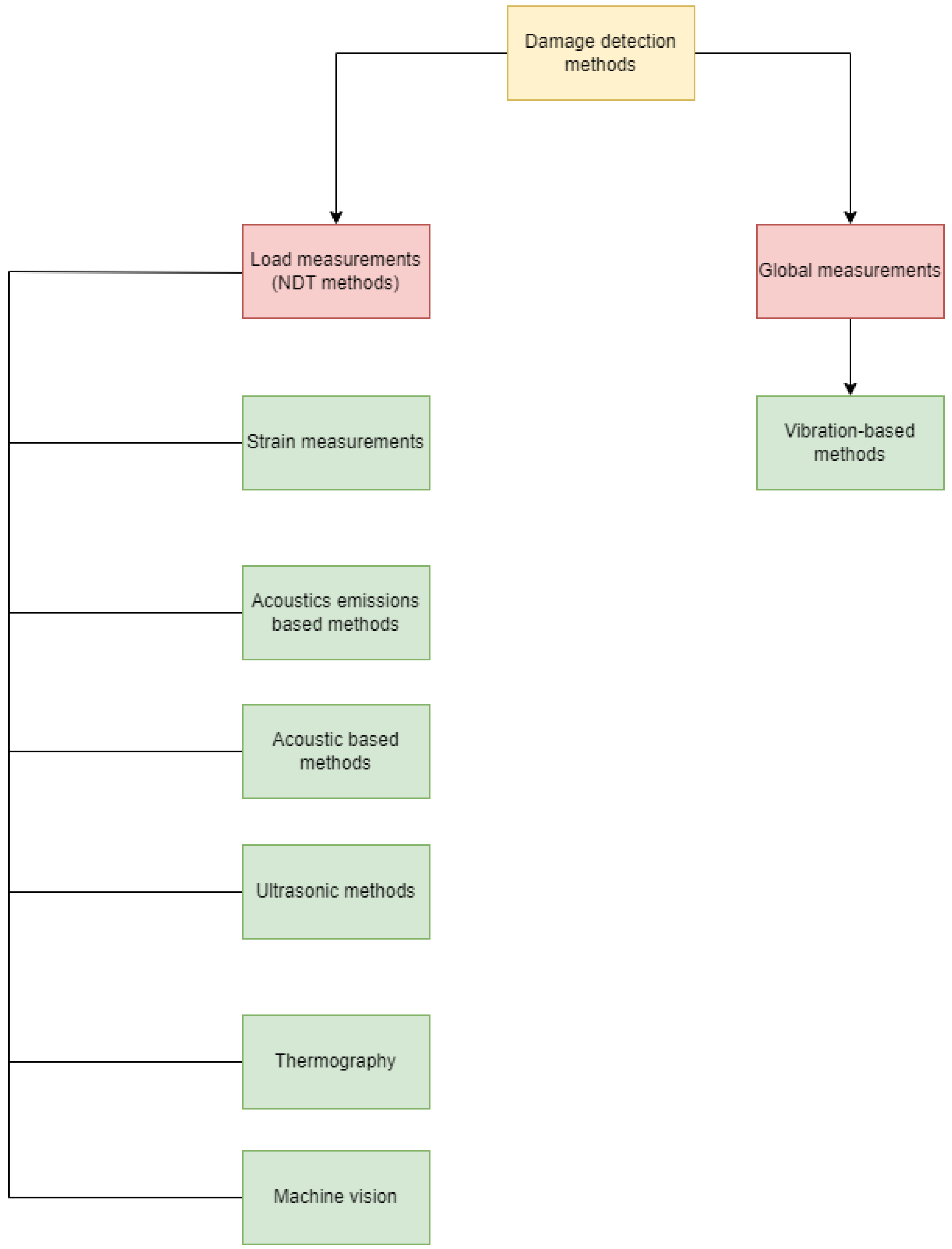
Figure 2.
Machine learning classification and main algorithms [60].
Figure 2.
Machine learning classification and main algorithms [60].
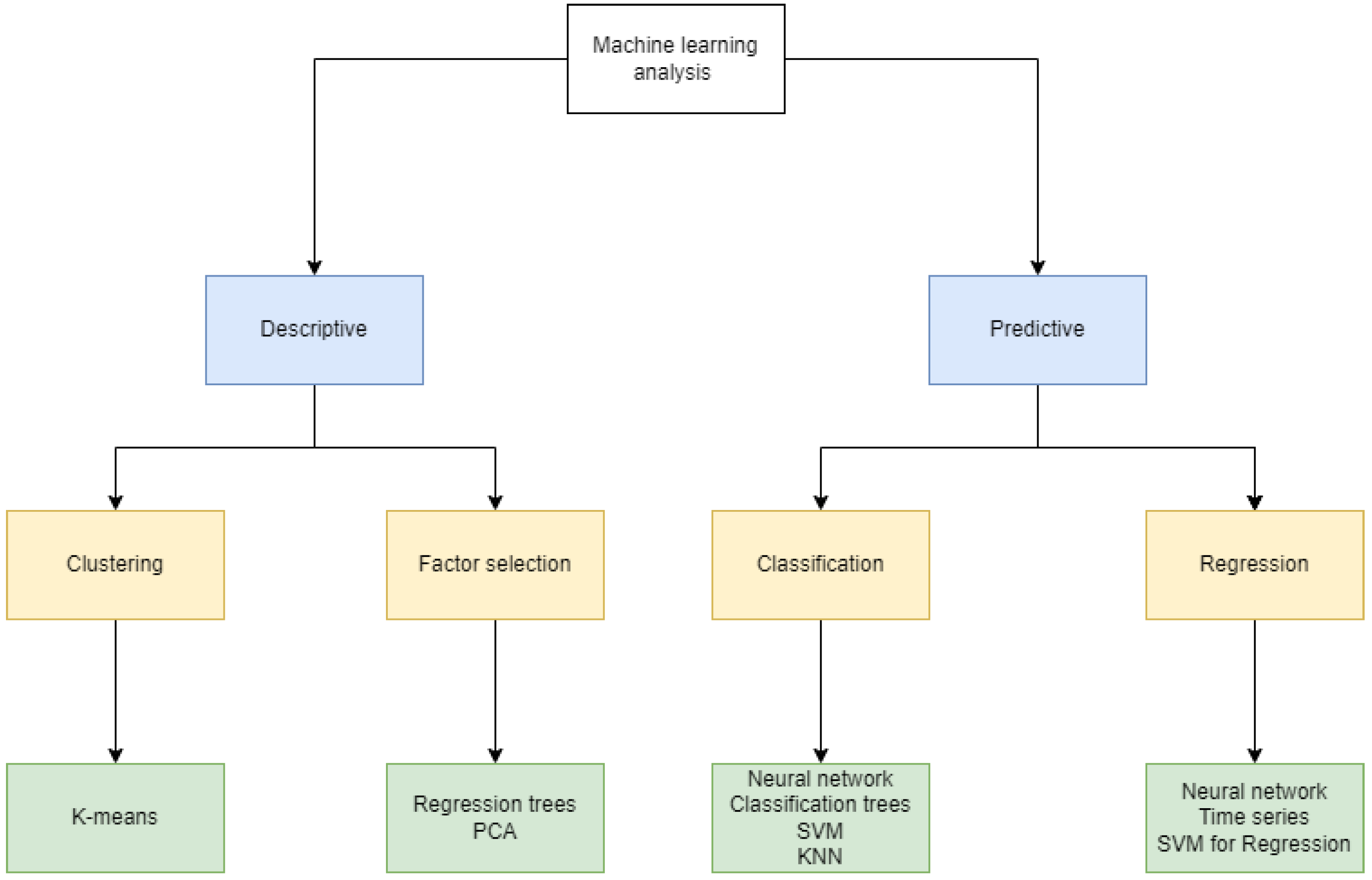
Figure 3.
Drawing views of the wing structure.
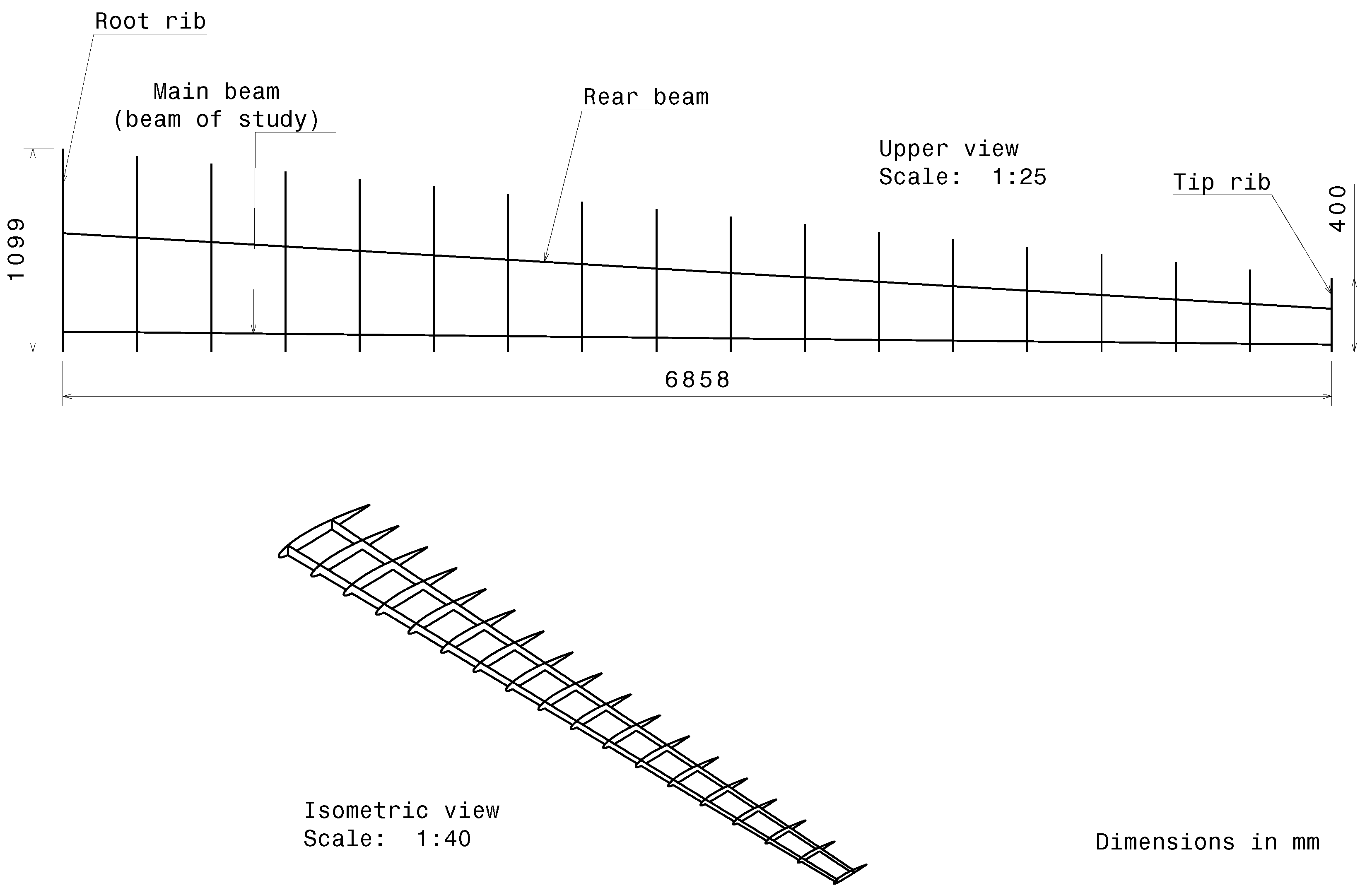
Figure 4.
Meshed geometry and detailed view of damages.
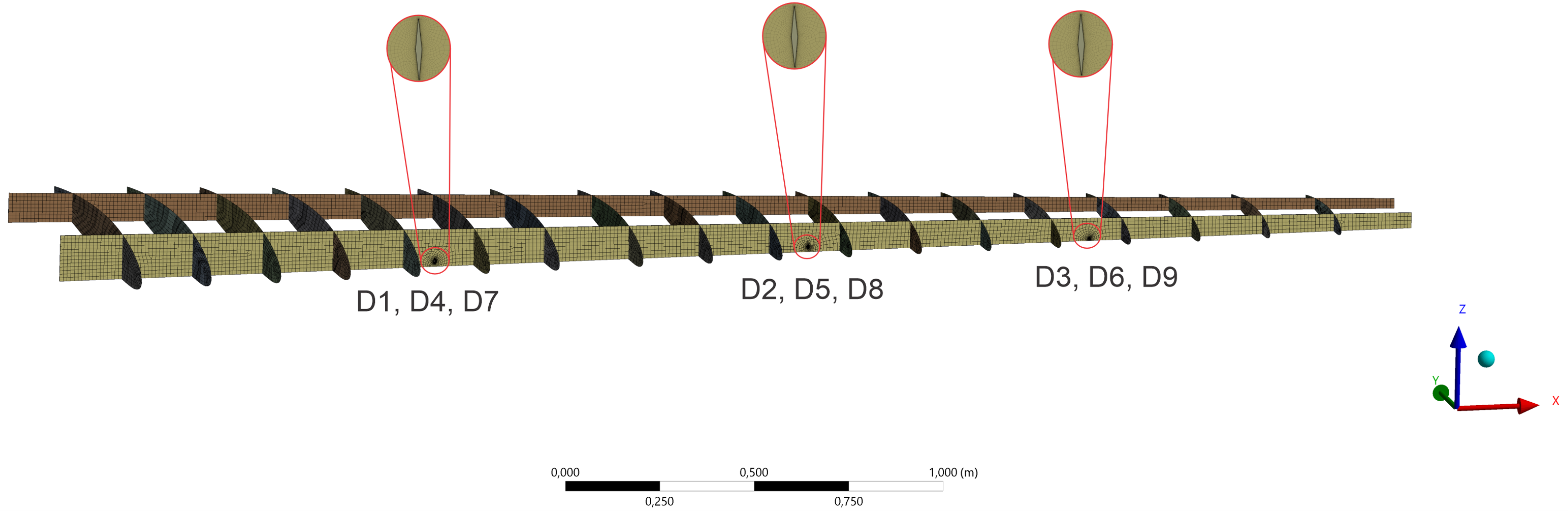
Figure 5.
20 mm hole and crack meshing.
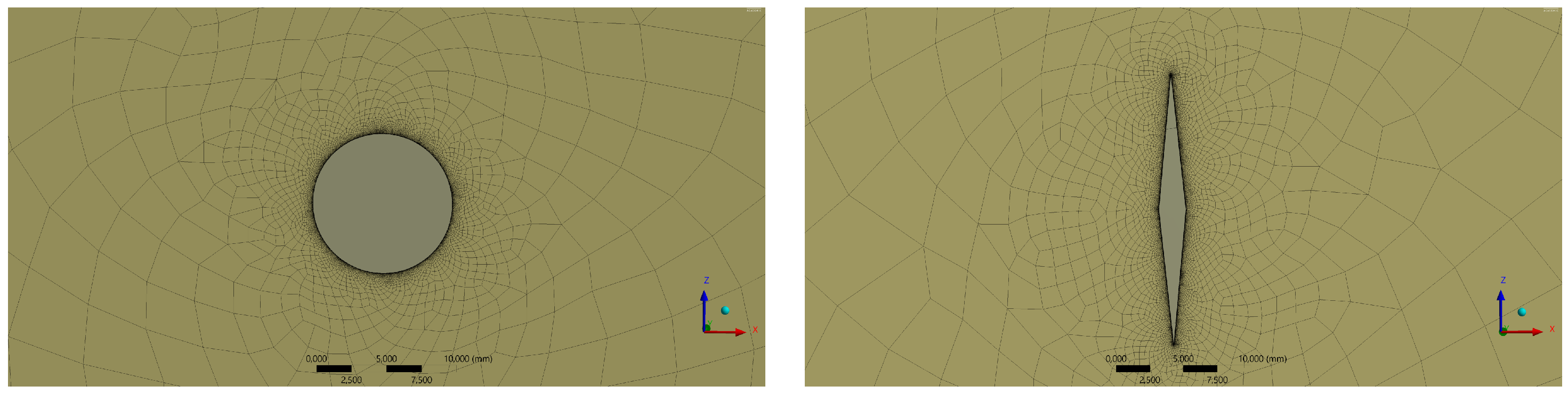
Figure 6.
Mesh convergence study.
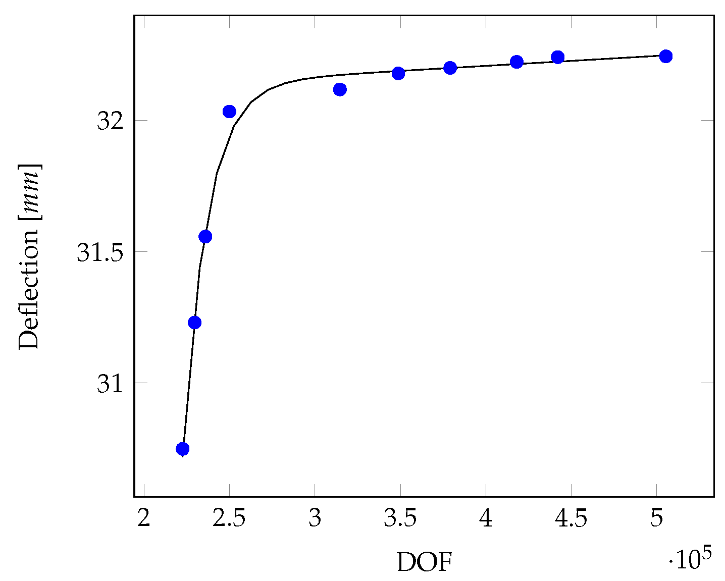
Figure 7.
Boundary conditions on validation model.
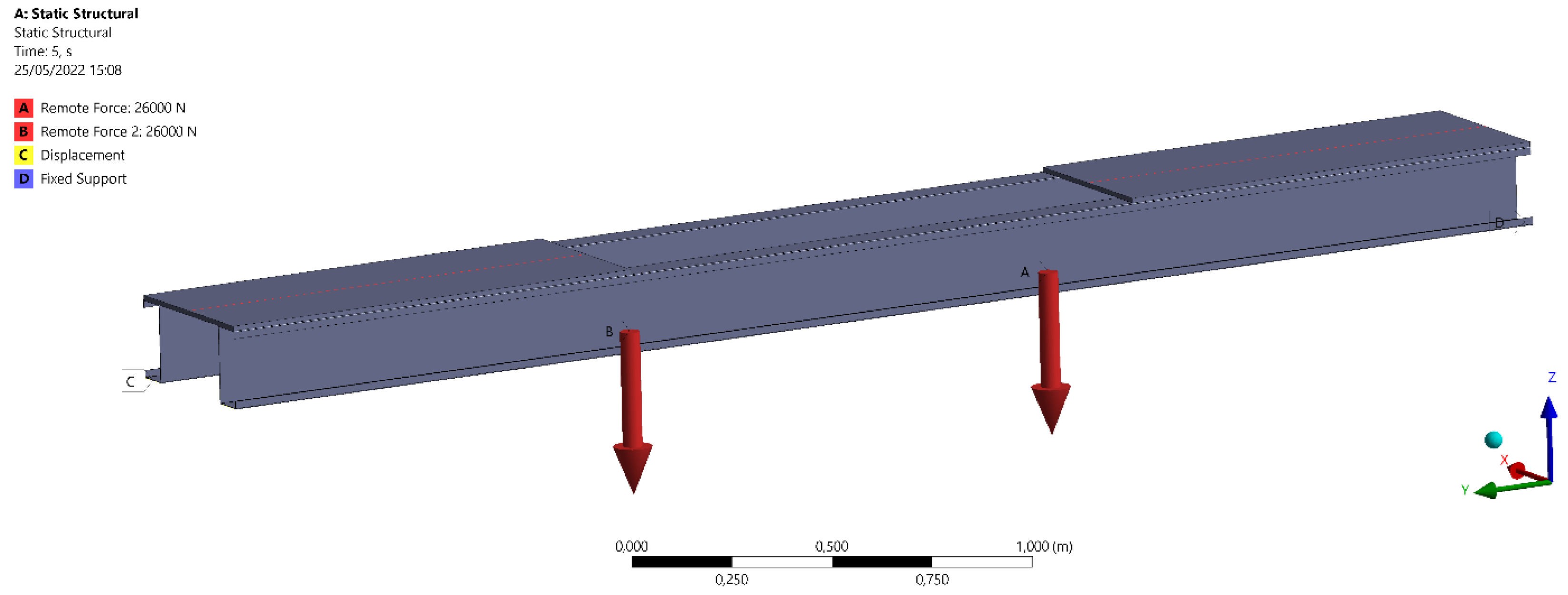
Figure 8.
Maximum moment applied.
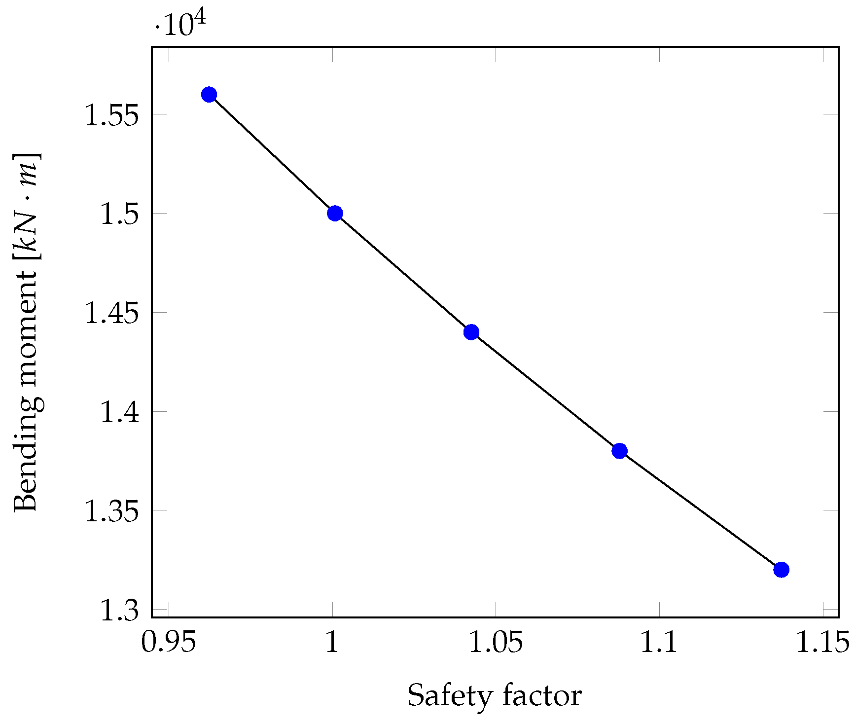
Figure 9.
Q statistic for Hole and crack
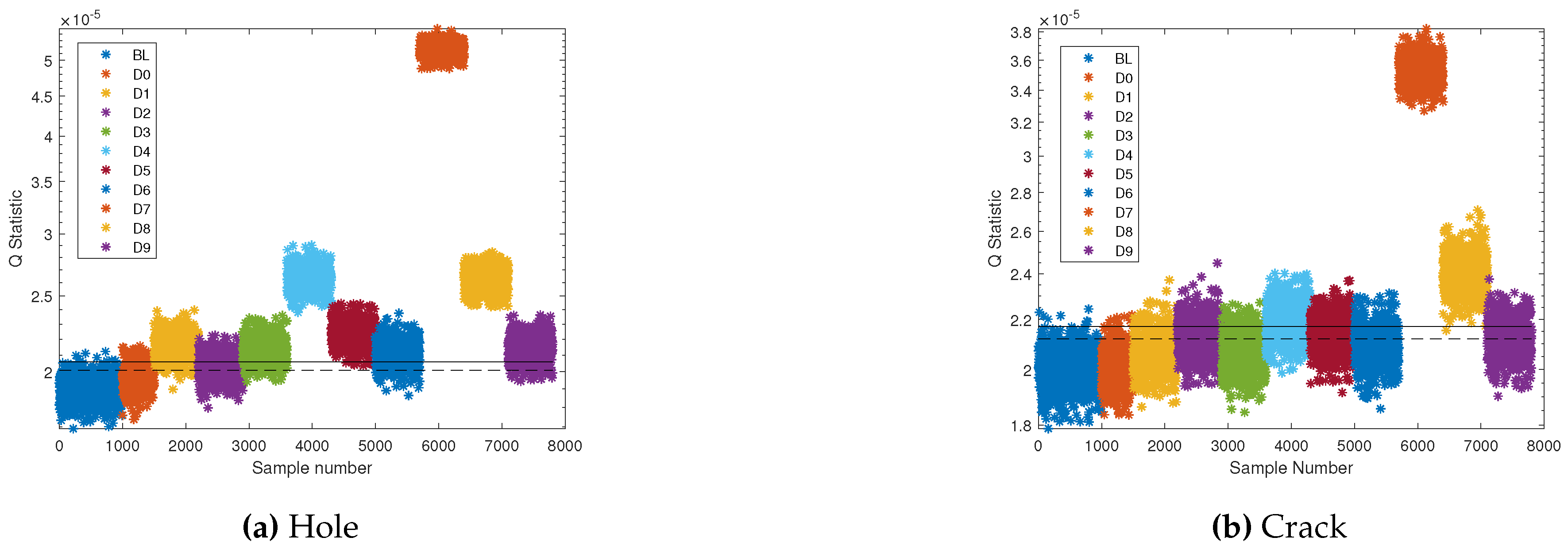
Figure 10.
Damage location comparison between lower and higher F1 values for hole.
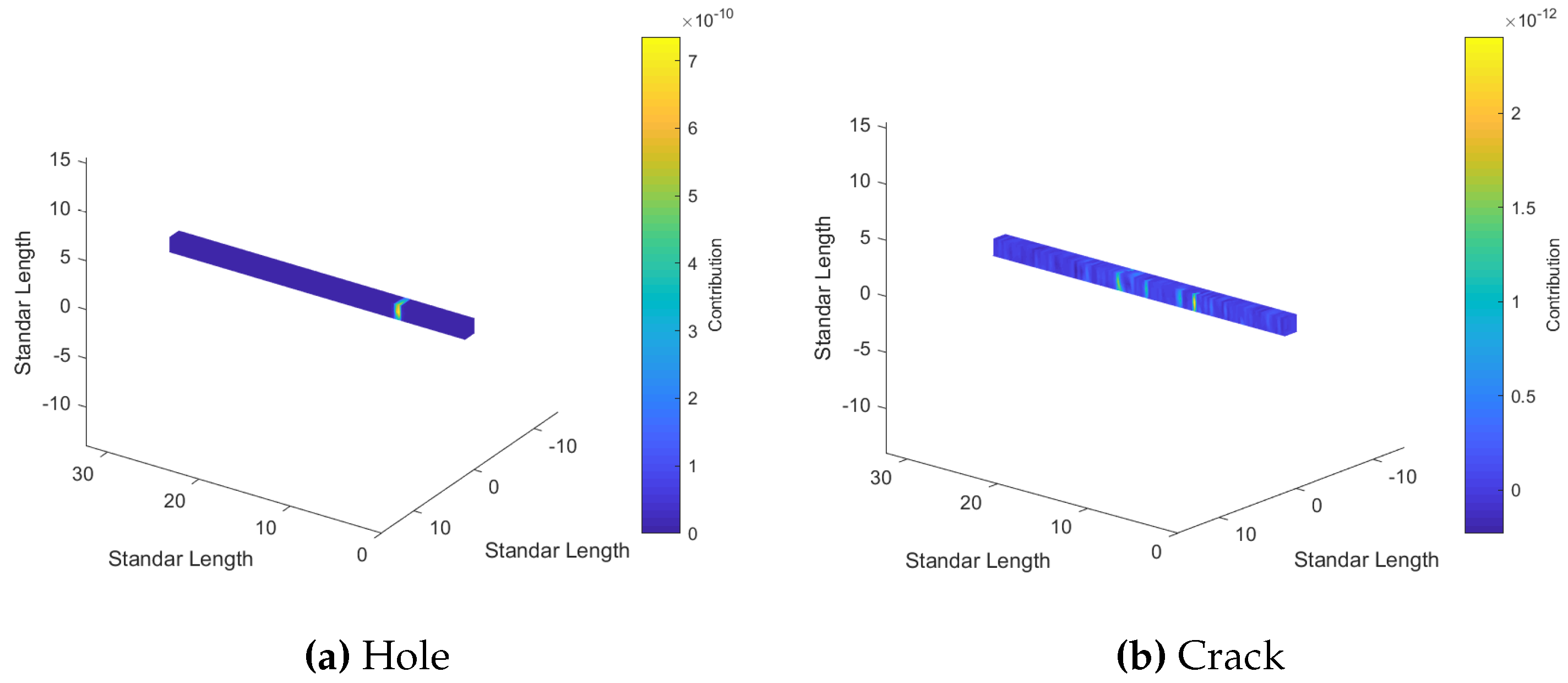
Figure 11.
Damage location comparison between lower and higher F1 values for crack.
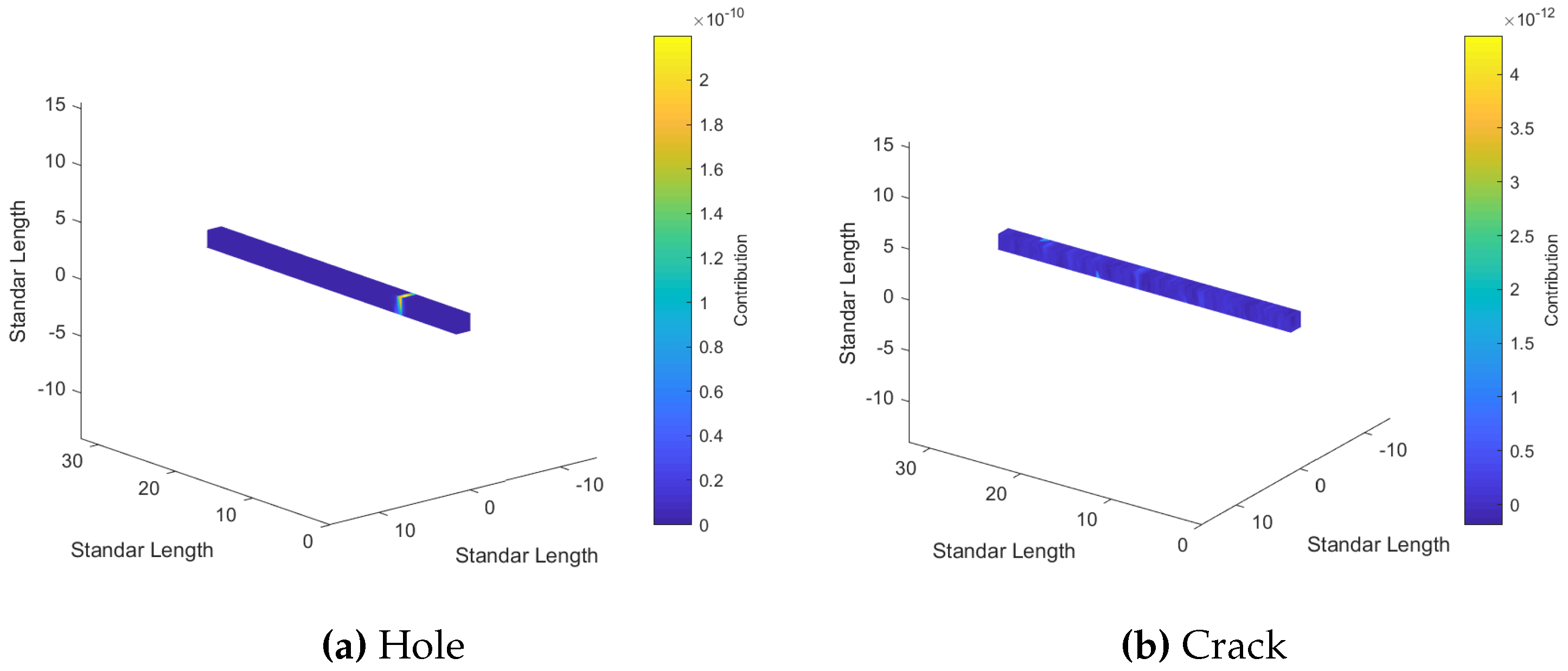
Figure 12.
Sensors removed for hole and crack.
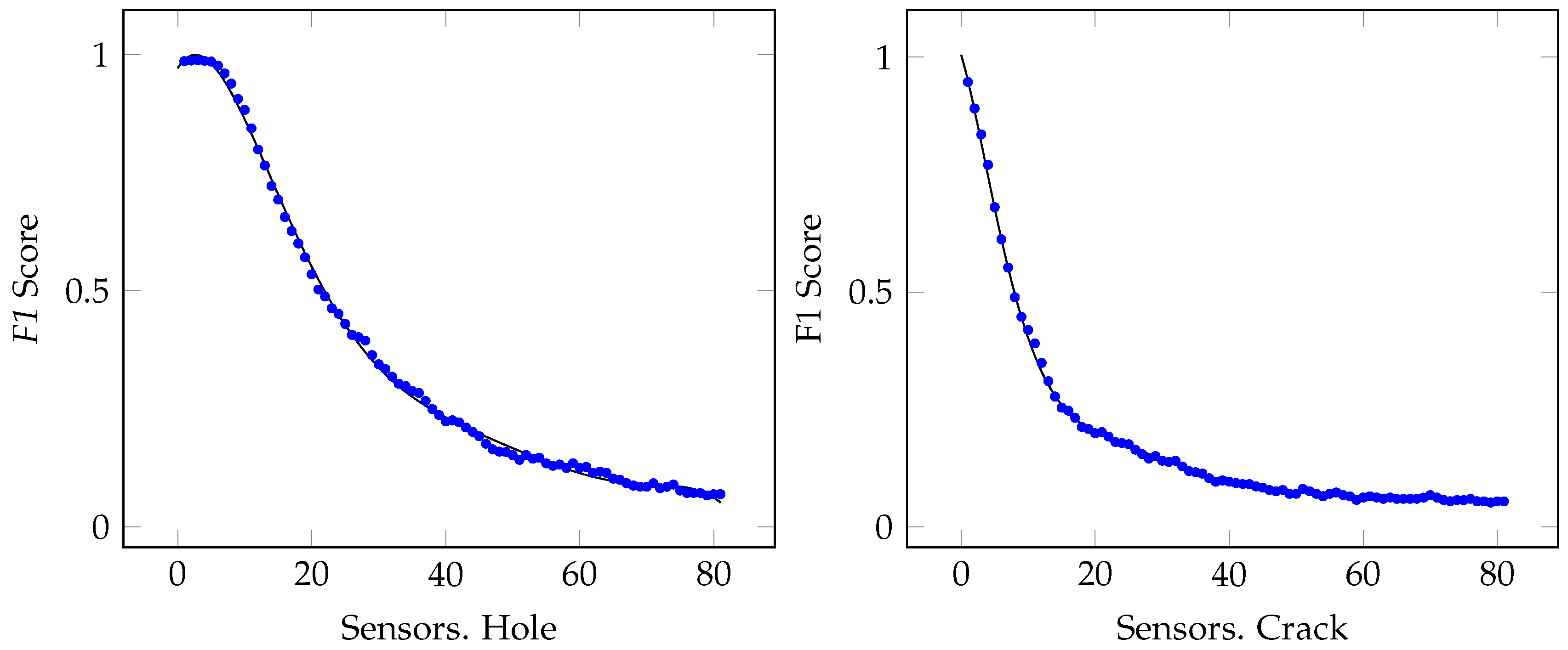
Figure 13.
Signal to noise ratio for hole and crack at damage D6.

Figure 14.
Signal to noise ratio for hole and crack at damage D6.
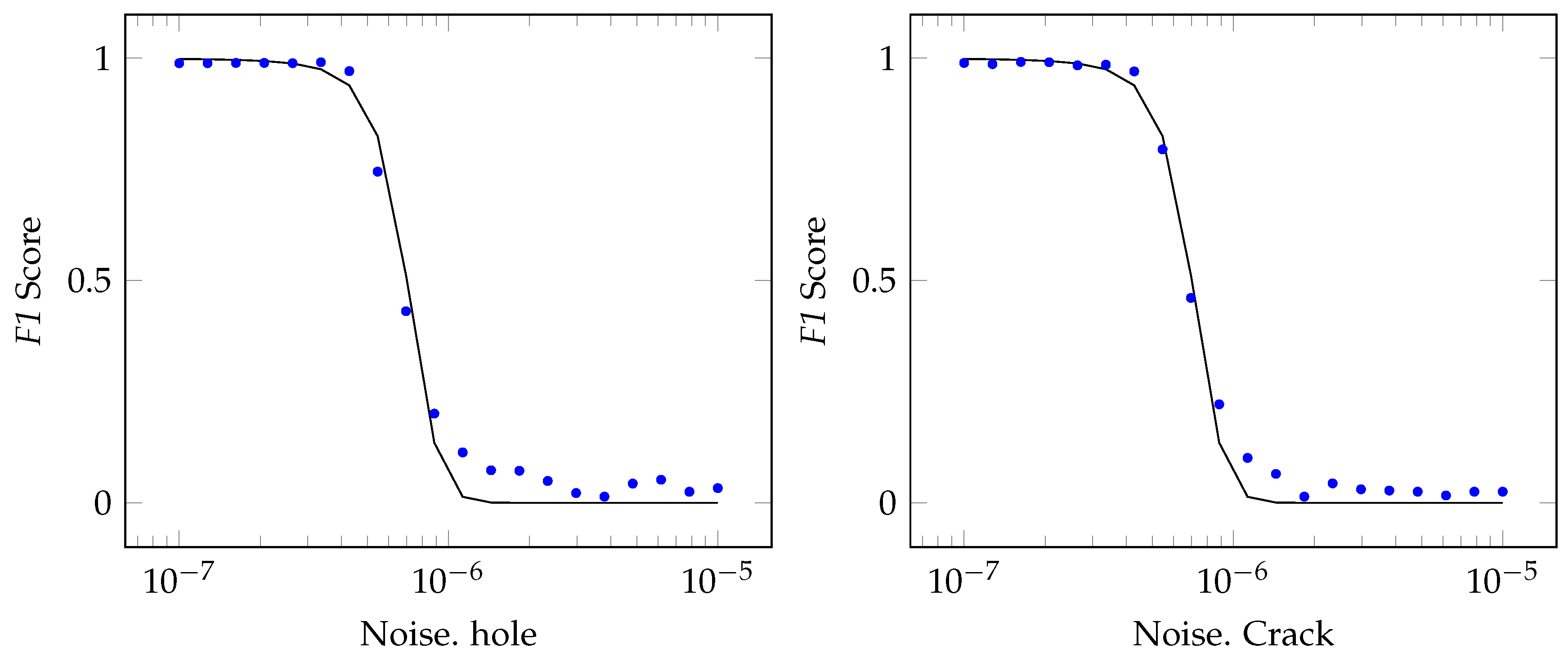

Table 1.
Damages locations and sizes.
| Size | |||
|---|---|---|---|
| Position | 2 mm | 10 mm | 20 mm |
| (% of wingspan) | |||
| 25% | D1 | D4 | D7 |
| 50% | D2 | D5 | D8 |
| 75% | D3 | D6 | D9 |
Table 2.
F1 score for crack damage.
| Size | |||
|---|---|---|---|
| Position | 2 mm | 10 mm | 20 mm |
| 25% | 0.0360 | 0.9936 | 0.9936 |
| 50% | 0.0468 | 0.8939 | 0.9936 |
| 75% | 0.1584 | 0.3850 | 0.6016 |
Table 3.
F1 score for hole damage.
| Size | |||
|---|---|---|---|
| Position | 2 mm | 10 mm | 20 mm |
| 25% | 0.6511 | 0.9852 | 0.9852 |
| 50% | 0.0976 | 0.9852 | 0.9852 |
| 75% | 0.2263 | 0.1770 | 0.9737 |
Table 4.
Most contributing sensors for crack damages.
| Size | |||
|---|---|---|---|
| Position | 2 mm | 10 mm | 20 mm |
| 25% | 322 | 321 | 321 |
| 50% | 347 | 347 | 148 |
| 75% | 68 | 373 | 373 |
Table 5.
Most contributing sensors for hole damages.
| Size | |||
|---|---|---|---|
| Position | 2 mm | 10 mm | 20 mm |
| 25% | 321 | 321 | 321 |
| 50% | 347 | 347 | 149 |
| 75% | 364 | 351 | 351 |
Disclaimer/Publisher’s Note: The statements, opinions and data contained in all publications are solely those of the individual author(s) and contributor(s) and not of MDPI and/or the editor(s). MDPI and/or the editor(s) disclaim responsibility for any injury to people or property resulting from any ideas, methods, instructions or products referred to in the content. |
© 2024 by the authors. Licensee MDPI, Basel, Switzerland. This article is an open access article distributed under the terms and conditions of the Creative Commons Attribution (CC BY) license (https://creativecommons.org/licenses/by/4.0/).
Copyright: This open access article is published under a Creative Commons CC BY 4.0 license, which permit the free download, distribution, and reuse, provided that the author and preprint are cited in any reuse.


