Submitted:
12 September 2025
Posted:
15 September 2025
You are already at the latest version
Abstract
This paper proposes a methodology based on the combined application of climate indices for precipitation and temperature along with multispectral Sentinel 2 imagery, used to generate vegetation indices that serve to diagnose the condition of subtropical irrigated crops through a predictive model. These crops demand significant irrigation, and in Mediterranean semi-arid environments, where water scarcity and drought periods are increasingly frequent and severe, this presents a serious problem. The aim of this methodological proposal is to address the need to adjust cultivated areas to actual water availability. It is now evident and necessary to implement efficient management of agricultural practices, avoiding the expansion of irrigated areas when there is not enough water available. As a result of this work, the climatic interrelation with the real condition of the crops is demonstrated.
Keywords:
1. Introduction
2. Materials and Methods
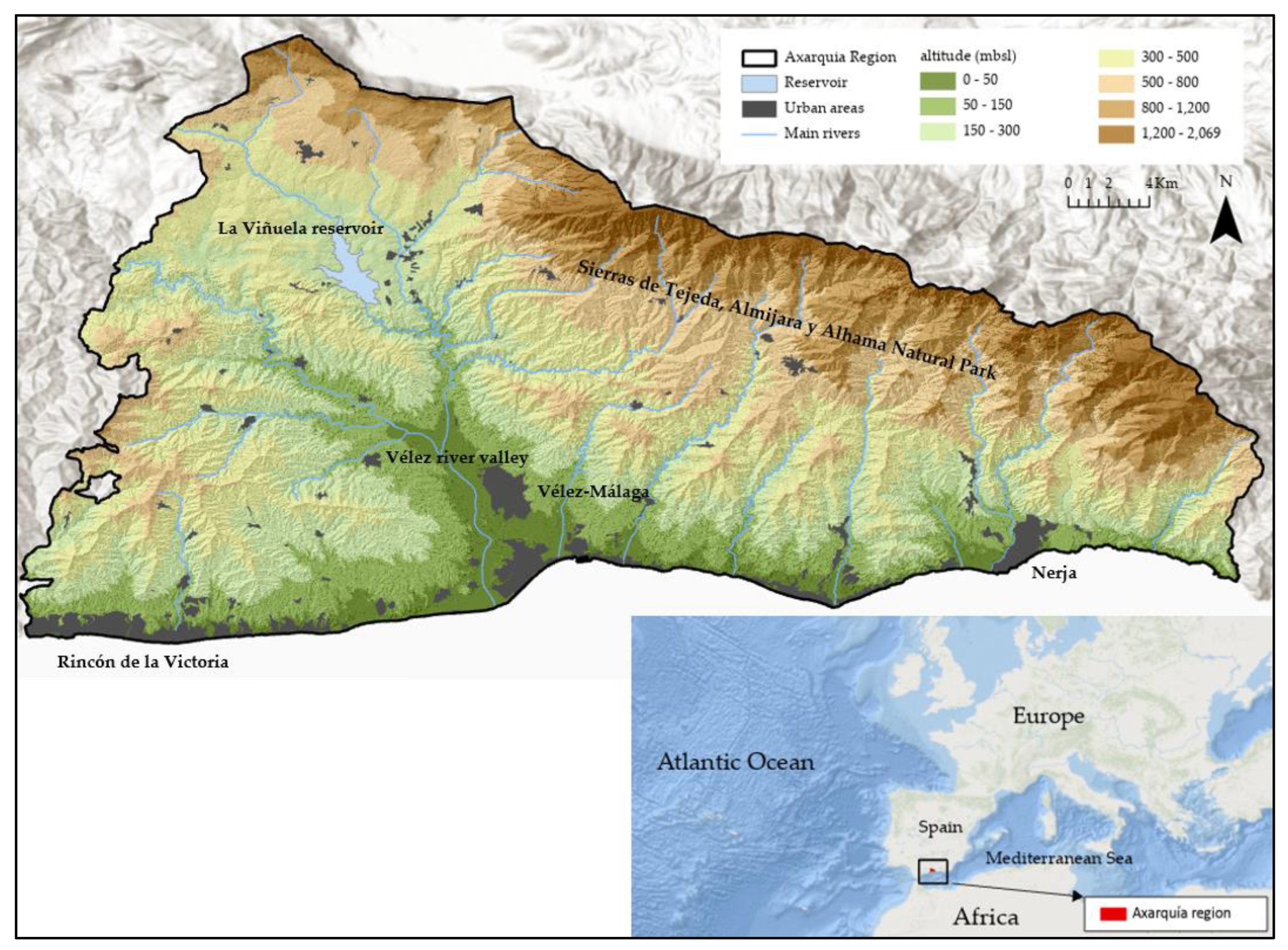
2.1. Study Area
2.2. Materials and Methods
2.3. Temporal Delimitation of Drought Periods
2.4. Satellite Image Acquisition and Processing
- 1)
- Download Sentinel 2A and 2B satellite images at Level L1C using the “Product Library” tool for the selected dates that include our study area, which is divided into two images.
- 2)
- Atmospheric correction of the images is performed with the “Sen2Cor” tool, upgrading them from Level L1C to Level L2A to enhance visualization.
- 3)
- Crop the images spatially and spectrally using the “Subset” tool, defining the study area and selecting the bands to be used—specifically bands 2, 3, 4, 8, and 11—to reduce data volume.
- 4)
- Standardize the spatial resolution of the spectral bands to 10 meters with the “Resampling” tool, since band 11 has a resolution of 20 meters and the rest are 10 meters.
- 5)
- Merge the two images that make up the study area with the “Mosaicking” tool, using the WGS84 projection, ortho-rectified with the Copernicus Global DEM at 30 meters and a pixel size of 10 meters.
- 1)
- Images were selected for the study’s temporal range: from 2015 (the earliest available images) to 2024. It was necessary to harmonize images taken before and after January 25, 2002, to ensure comparability, as changes in image processing within the Copernicus program— which began generating images with new radiometric calibration— directly affected temporal image analysis, especially when conducting comparisons of vegetation indices as in this case.
- 2)
- Images from the area of interest were chosen by selecting only the tile or tiles (100x100 km2 grid images, orthorectified in UTM/WGS84 projection) that encompass the study area, thus providing the input geometry.
- 3)
- A clip was performed using this input geometry, cropping the 100x100 km2 images to only the area corresponding to the specific crop and variety under study. This approach allows for an accurate assessment of the heterogeneity in crop evolution, minimizing interference from other crop types or varieties. Achieving data homogeneity is essential.
- 4)
- Pixels associated with water vapor (clouds) were removed, as their reflectance does not represent the surface of interest and would generate negative values when analyzing vegetation indices. To achieve this, Sentinel-2 Level-2A’s QA60 band is used—see Table 2 for a simplified overview of the filtering criteria—by which a straightforward function is created for cloud masking. Technically, QA60 is not a true spectral band but rather reuses two far-infrared water vapor reflectance bands. The source bands are B10 and B11, with the QA60 service flagging, via a Boolean filter, any bits where opaque clouds are present. With this, we can assess each image, apply all previous filters, and finally apply this last step, which removes all pixels where QA60 indicates opaque clouds.
- 5)
- When applying a bitmask for QA60, each image must be processed sequentially by date, applying the cloud-masking algorithm, and saving it with its corresponding date and without clouds. If a particular image is fully cloud-covered, it is excluded from the image collection. If it is mostly clear, it is retained, and for images with a certain proportion of removed pixels, their influence will be weighted accordingly in subsequent mean calculations.
- (1)
- Bitmask for QA60.
2.5. Image Analysis, Application of Spectral Indexes and Statistical Analysis
2.6. Classification of Indexes, Cluster Analysis and Mapping
- 1)
- For vegetation indices focused on detecting crop health and vigor, a distinction is made between crops with low and high vegetation cover, taking into account that young plantations may be included among those with low cover.
- 2)
- For vegetation indices measuring canopy and soil moisture content, a differentiation is established between irrigated and non-irrigated crops, as well as the water stress they may experience due to a lack of water or insufficient irrigation.
- 1)
- Disposition, quantification, and evolution of the crop. Understanding physical aspects is essential both to comprehend how the crop responds to specific events and interventions, and to interpret monitoring results. To achieve this, a temporal sequence of RGB images is conducted. This analysis allows for observation of crop evolution and temporal variability, enabling detection of possible impacts suffered by the crop, its response to solutions or management techniques applied in the field, correlation of crop behavior in areas with different productivity, as well as the recording of this information for comparison at different times.
- 2)
- Study of crop behavior according to the different growth cycles during the same season. Throughout the production months, information is obtained to assess the state, variability, and evolution of crop vigor and water status, with the aim of detecting impacts and anomalies.
- 3)
- Crop characterization. This is carried out considering three variables: Tree Count Management, Tree Height Measurement, and Erosion Risk, with the intention of evaluating the homogeneity of the cultivated area under analysis.
3. Results
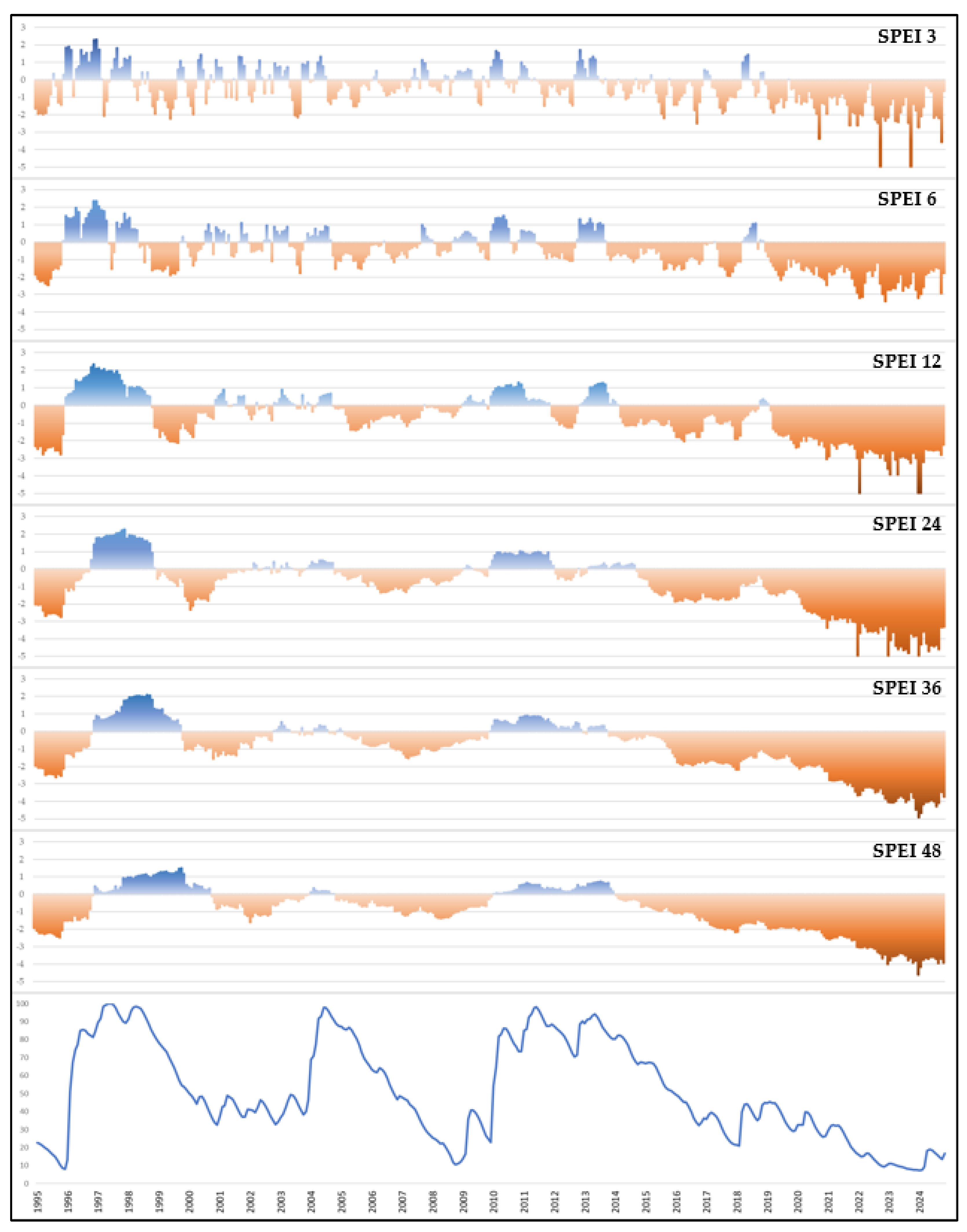
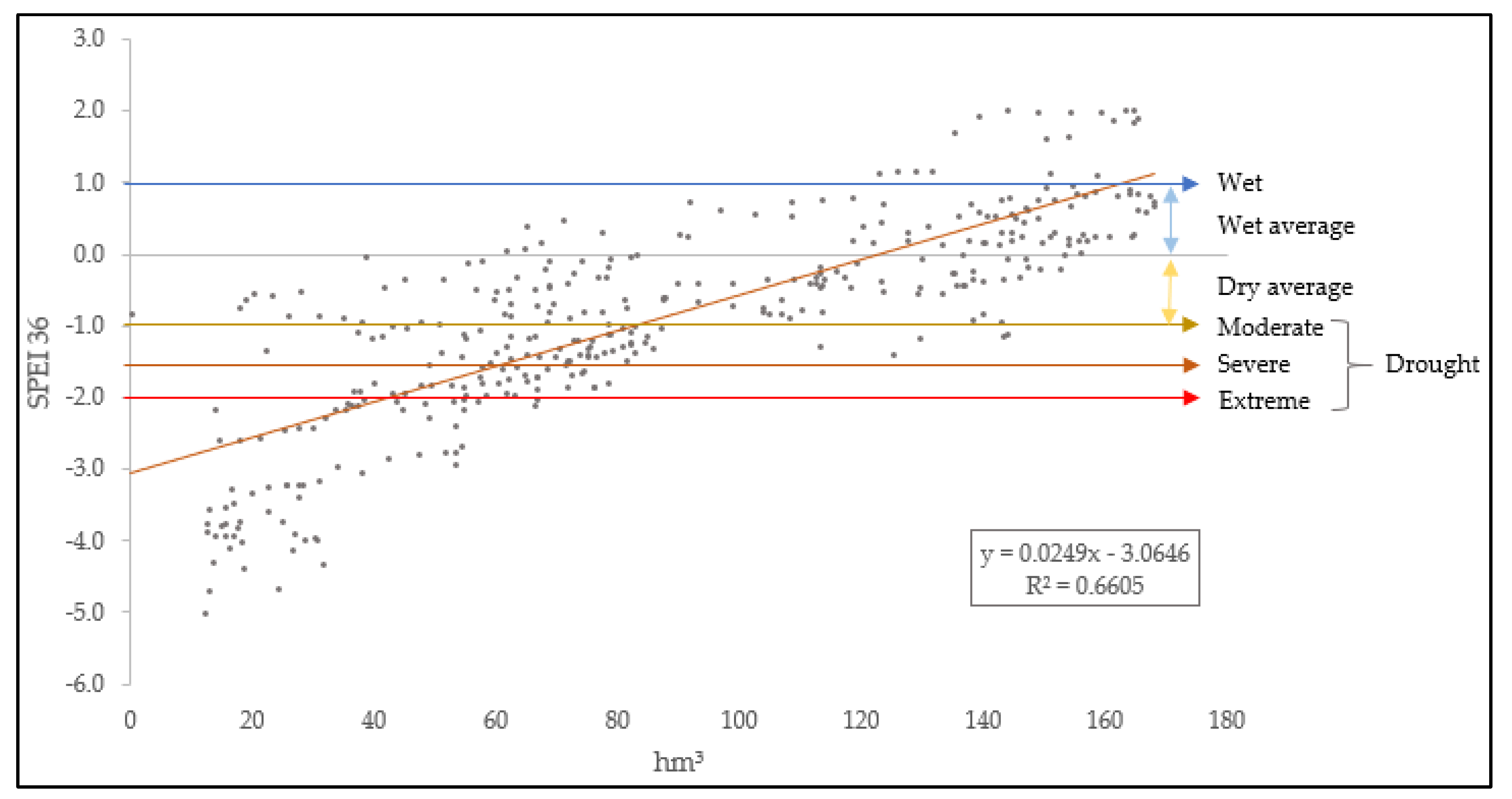
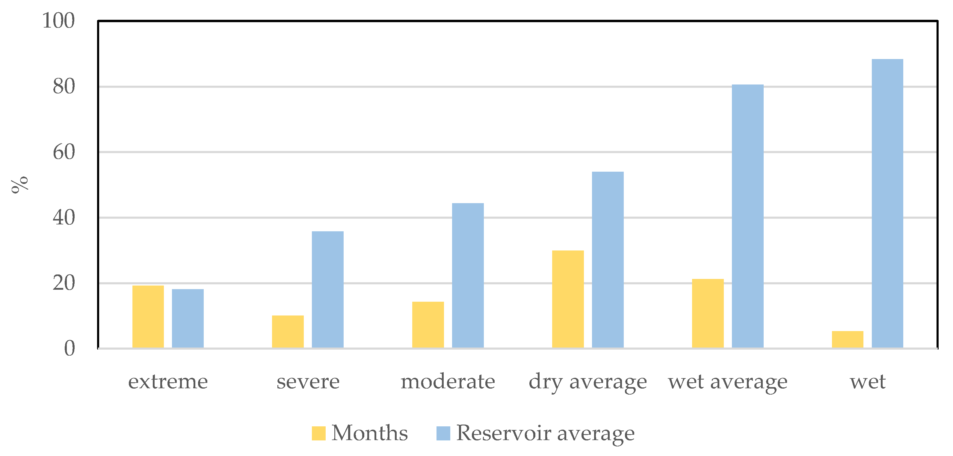
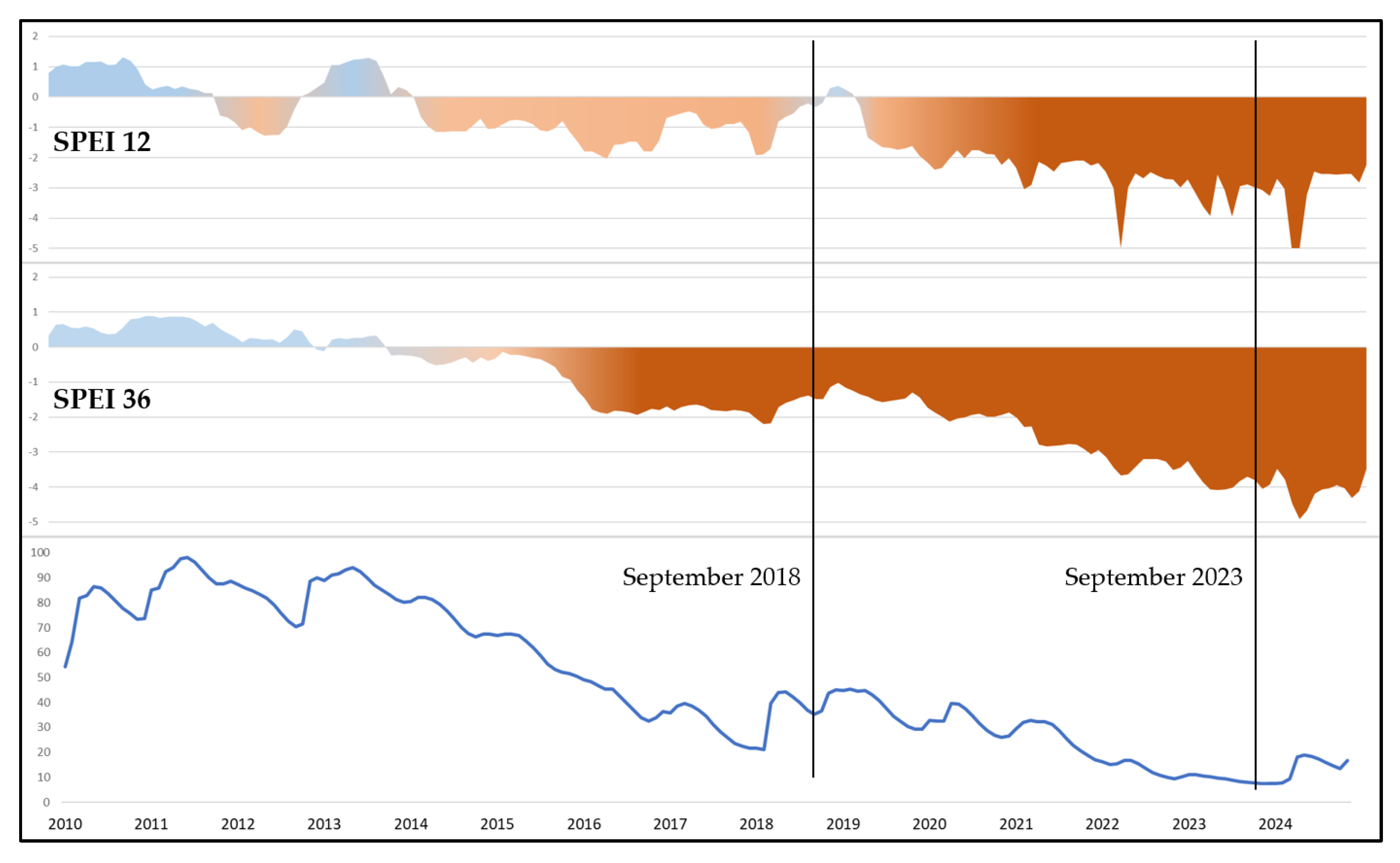
3.1. Temporal Analysis of Drought
3.2. Statistical Analysis, Classification and Clustering of Spectral Indices
- 1)
- Planting season. Takes place from spring through early summer. Spacing begins at 4x4 m² to 8x8 m², or even 4x8 m², and when the trees grow and their canopies touch, the center tree is removed. This, of course, determines the spectral response. In addition to the planting framework, several conditions must be understood for optimal plant development: soil status, moisture conditions, and the climate balance.
- 2)
- Harvest season. Fruit is collected from November through May. Harvest usually starts in November, but only if fruit drops or if it has grown substantially. Most commonly, the harvest begins in December and ends by late April, though these dates can shift based on the year and temperature, as leaving fruit on the tree influences flowering. At this stage, it is crucial to track the overall health of the plant.
- 3)
- Pruning stage. Performed twice a year: once at the end of winter (March) and once in summer (July/August), though some growers carry out pruning in September. Notably, August is usually a critical month in most Mediterranean climate cultivation zones, as not only can the developing fruit deteriorate due to heat, but the plant itself also suffers from water stress.
- 4)
- Flowering stage. Typically occurs in spring, in March and April. In semi-arid regions, flowering coincides with rising temperatures, making it necessary to monitor conditions closely to ensure this process unfolds as desired, especially since after these months (June–July) fruit drop can increase due to heat and the small size of young fruits.
- 5)
- Fertilization period. Generally, three applications are made: one at the onset of the rainy season (late September/October) and two more every two months (December and February). It is important to monitor this process, as fertilization is often carried out indiscriminately, without considering the diverse soil conditions.

| Vegetation Index | Classification | Value | Description | 2018 ha | 2018 % | 2023 ha | 2023 % | ||||
|---|---|---|---|---|---|---|---|---|---|---|---|
| NDVI | 1 | -1 — 0.15 | uncultivated area | 450.90 | 3.53 | 1,998.47 | 13.9 | ||||
| 2 | 0.15 — 0.30 | low cover crop | 2,612.02 | 20.43 | 5,887.73 | 41.00 | |||||
| 3 | 0.30 — 0.45 | medium cover crop | 2,914.94 | 22.80 | 3,954.84 | 27.50 | |||||
| 4 | 0.45 — 0.60 | medium/high cover crop | 2,538.37 | 19.85 | 2,176.69 | 15.14 | |||||
| 5 | 0.60 — 1 | high cover crop | 4,269.11 | 33.39 | 354.83 | 2.47 | |||||
| NDMI | 1 | -1 — 0 | non-irrigated area | 4,714.05 | 36.87 | 5,443.32 | 37.87 | ||||
| 2 | 0 — 1 | irrigated area | 8,071.30 | 63.13 | 8,929.24 | 62.13 | |||||
| MSI | 1 | 0.16 — 0.90 | crops without water stress | 6,654.04 | 52.04 | 6,131.28 | 42.66 | ||||
| 2 | 0.9 — 1.3 | slightly water-stressed crops | 4,754.9 | 37.19 | 7,930.97 | 55.18 | |||||
| 3 | 1.3 — 1.9 | moderate water-stressed crops | 1,359.11 | 10.63 | 309.99 | 2.16 | |||||
| 4 | 1.9 — 2.5 | extremely water-stressed crops | 16.42 | 0.13 | 0.32 | 0.00 | |||||
| 5 | >2.5 | water | 0.87 | 0.007 | 0.00 | 0.00 | |||||
3.3. Mapping
4. Discussion
5. Conclusions
Author Contributions
Funding
Data Availability Statement
Conflicts of Interest
Abbreviations
| BOA | Bottom of Atmosphere |
| ESA | European Space Agency |
| GNDVI | Green Normalized Difference Vegetation Index |
| GSI | Grain Size Index |
| KMO | Kaiser-Meyer-Olkin method |
| LAI | Leaf Area Index. |
| MSI | Moisture index |
| NDDI | Normalized Difference Drought Index |
| NDMI | Normalized Difference Moisture Index |
| NDVI | Normalized Difference Vegetation Index |
| NDW1 | Normalized Difference Water Index |
| SAIH | Sistema Automático de Información Hidrológica |
| SNAP | Sentinel Application Platform |
| SPEI | Standardised Precipitation-Evapotranspiration Index |
| SPI | Standardized Precipitation Index |
| SIPNA | Sistema de Información sobre el Patrimonio Natural de Andalucía |
| SPSS | Statistical Package for the Social Sciences |
| TOA | Top of Atmosphere |
| WMO | World Meteorological Organization |
References
- Gosling, S. N.; Arnell, N. W. A global assessment of the impact of climate change on water scarcity. Climatic Change 2016, 134, 371–385. [Google Scholar] [CrossRef]
- Hoerling, M.; Eischeid, J.; Perlwitz, J.; Quan, X.; Zhang, T.; Pegion, P. On the increased frequency of Mediterranean drought. Journal of climate 2012, 25, 2146–2161. [Google Scholar] [CrossRef]
- Sousa, P. M.; Trigo, R. M.; Aizpurua, P.; Nieto, R.; Gimeno, L.; Garcia-Herrera, R. Trends and extremes of drought indices throughout the 20th century in the Mediterranean. Natural Hazards and Earth System Sciences 2011, 11, 33–51. [Google Scholar] [CrossRef]
- Le, T.S.; Harper, R.; Dell, B. Application of Remote Sensing in Detecting and Monitoring Water Stress in Forests. Remote Sens. 2023, 15, 3360. [Google Scholar] [CrossRef]
- Carella, A.; Bulacio Fischer, P.T.; Massenti, R.; Lo Bianco, R. Continuous Plant-Based and Remote Sensing for Determination of Fruit Tree Water Status. Horticulturae 2024, 10, 516. [Google Scholar] [CrossRef]
- Vicente-Serrano, S. M.; Lopez-Moreno, J. I.; Beguería, S.; Lorenzo-Lacruz, J.; Sanchez-Lorenzo, A.; García-Ruiz, J. M.; Espejo, F. Evidence of increasing drought severity caused by temperature rise in southern Europe. Environmental Research Letters 2014, 9, 044001. [Google Scholar] [CrossRef]
- Salas-Martínez Fernando, Valdés-Rodríguez Ofelia Andrea, Palacios-Wassenaar Olivia Margarita, Márquez-Grajales Aldo, Rodríguez-Hernández Leonardo Daniel. Methodological estimation to quantify drought intensity based on the NDDI index with Landsat 8 multispectral images in the central zone of the Gulf of Mexico. Frontiers in Earth Science 2023, 11, 1–13. [Google Scholar] [CrossRef]
- Jonathan Spinoni, Paulo Barbosa, Alfred De Jager, Niall McCormick, Gustavo Naumann, Jürgen V. Vogt, Diego Magni, Dario Masante, Marco Mazzeschi, A new global database of meteorological drought events from 1951 to 2016. Journal of Hydrology: Regional Studies 2019, 22, 100593. [CrossRef]
- Francisco José Del-Toro-Guerrero, Thomas Kretzschmar, Precipitation-temperature variability and drought episodes in northwest Baja California, México, Journal of Hydrology: Regional Studies 2020, 27, 2020, 100653. [CrossRef]
- Kaoutar Mounir, Isabelle La Jeunesse, Haykel Sellami, Abdessalam Elkhanchoufi. Spatiotemporal analysis of drought occurrence in the Ouergha catchment, Morocco[J]. AIMS Environmental Science, 2023; 10, 398–423. [CrossRef]
- G. Legesse, K.V. Suryabhagavan. Remote sensing and GIS based agricultural drought assessment in East Shewa Zone. Ethiopia. Tropical Ecology 2014, 55, 349–363. Available online: https://www.researchgate.net/publication/239791588_Remote_sensing_and_GIS_based_agricultural_drought_assessment_in_East_Shewa_Zone_Ethiopia.
- Ruiz-Sinoga, J. D.; Garcia-Marin, R.; Gabarron-Galeote, M. A.; Martinez-Murillo, J. F. Analysis of dry periods along a pluviometric gradient in Mediterranean southern Spain. International Journal of Climatology 2012, 32. [Google Scholar] [CrossRef]
- Rodríguez Díaz, J. A.; Weatherhead, E. K.; Knox, J. W.; Camacho, E. Climate change impacts on irrigation water requirements in the Guadalquivir River basin in Spain. Regional Environmental Change 2007, 7, 149–159. [Google Scholar] [CrossRef]
- FAOSTAT (2016) Food and Agriculture Organization of the United Nations (FAO). FAOSTAT Database. Available online: http://faostat.fao.org/site/291/default.aspx (accessed on 6 August 2025).
- European Environment Agency Climate change, impacts and vulnerability in Europe 2016 An indicator-based report 2017. [CrossRef]
- Ergene, Emine & Balcik, Filiz & Şanlı, F. Trends analysis of agricultural drought in central anatolian basin, Turkey. The International Archives of the Photogrammetry, Remote Sensing and Spatial Information Sciences 2024. XLVIII-4/W9-2024. 141-148. 10.5194/isprs-archives-XLVIII-4-W9-2024-141-2024. [CrossRef]
- Li, T.; Zhong, S. Advances in Optical and Thermal Remote Sensing of Vegetative Drought and Phenology. Remote Sens. 2024, 16, 4209. [Google Scholar] [CrossRef]
- Schillinger, W. F.; Schofstoll, S. E.; Alldredge, J. R. Available water and wheat grain yield relations in a Mediterranean climate. Field Crops Research 2008, 109, 45–49. [Google Scholar] [CrossRef]
- Austin, R. B.; Cantero-Martınez, C.; Arrúe, J. L.; Playán, E.; Cano-Marcellán, P. Yield–rainfall relationships in cereal cropping systems in the Ebro River valley of Spain. European Journal of Agronomy 1998, 8, 239–248. [Google Scholar] [CrossRef]
- Li, Z.; Zhou, T.; Zhao, X.; Huang, K.; Wu, H.; Du, L. Diverse spatiotemporal responses in vegetation growth to droughts in China. Environmental Earth Sciences 2016, 75, 1–13. [Google Scholar] [CrossRef]
- Intergovernmental Panel on Climate Change (IPCC). Climate Change 2021 – The Physical Science Basis: Working Group I Contribution to the Sixth Assessment Report of the Intergovernmental Panel on Climate Change. Cambridge University Press; 2023. Available online: https://www.ipcc.ch/report/ar6/wg1/ (accessed on 6 August 2025).
- Rosa, L.; Chiarelli, D. D.; Rulli, M. C.; Dell’Angelo, J.; D’Odorico, P. Global agricultural economic water scarcity. Science Advances 2020, 6, eaaz6031. [Google Scholar] [CrossRef]
- Ramos, R. Y.; Romero, Ó. C.; Camacho, V. F.; Delgado, M. T. The bubble of subtropical crops and the water collapse in the Axarquía. In Gabinete de Estudios de la Naturaleza de la Axarquía (GENA), Vélez-Málaga (Spain), 2020. Available online: https://euroweeklynews.com/2024/02/24/the-subtropical-bubble-impacting-axarquias-water-crisis/ (accessed on 6 August 2025).
- Garau, E.; Vila-Subirós, J.; Palom, A. R. Agua, turismo y servicios de los ecosistemas: el ciclo hidroturístico en la cuenca mediterránea. In Challenges and opportunities of a world in transition. An interpretation from Geography, 1st ed.; Escribano, J., Peñarrubia, M.P., Serrano, J., Asins, S., Eds.; Tirant lo Blanc: Spain, 2020; Volume 1, pp. 251–264. Available online: https://www.researchgate.net/publication/344375258_Agua_turismo_y_servicios_de_los_ecosistemas_el_ciclo_hidroturistico_en_la_cuenca_mediterranea (accessed on 6 August 2025).
- Ibrahim, G.R.F.; Rasul, A. & Abdullah, H. Assessing how irrigation practices and soil moisture affect crop growth through monitoring Sentinel-1 and Sentinel-2 data. Environ Monit Assess 2023, 195, 1262. [Google Scholar] [CrossRef]
- Ma, C.; Johansen, K.; McCabe, M. F. Monitoring irrigation events and crop dynamics using Sentinel-1 and Sentinel-2 time series. Remote Sensing 2022, 14, 5. [Google Scholar] [CrossRef]
- Farid, H. U.; Khan, Z. M.; Shakoor, A.; Mubeen, M.; Ayub, H. U.; Kanwar, R. M. A.; Bilal, M. (2022). Water Resources in Relation to Climate Change. In: Jatoi, W.N.; Mubeen, M.; Ahmad, A.; Cheema, M.A.; Lin, Z.; Hashmi, M.Z. (eds). Building Climate Resilience in Agriculture. Springer, Cham.; 145-166. [CrossRef]
- Davarpanah, R.; Ahmadi, S. H. Modeling the effects of irrigation management scenarios on winter wheat yield and water use indicators in response to climate variations and water delivery systems. Journal of Hydrology 2021, 598, 126269. [Google Scholar] [CrossRef]
- Kharrou, M. H.; Simonneaux, V.; Er-Raki, S.; Le Page, M.; Khabba, S.; Chehbouni, A. Assessing irrigation water use with remote sensing-based soil water balance at an irrigation scheme level in a semi-arid region of Morocco. Remote Sensing 2021, 13, 1133. [Google Scholar] [CrossRef]
- Zuazo, V. H. D.; García-Tejero, I. F.; Rodríguez, B. C.; Tarifa, D. F.; Ruiz, B. G.; Sacristán, P. C. Deficit irrigation strategies for subtropical mango farming. A review. Agronomy for sustainable development 2021, 41, 13. [Google Scholar] [CrossRef]
- Bastiaanssen, W. G.; Molden, D. J.; Makin, I. W. Remote sensing for irrigated agriculture: examples from research and possible applications. Agricultural water management 2000, 46, 137–155. [Google Scholar] [CrossRef]
- FAO. Agricultural Value Chain Study in Iraq—Dates, Grapes, Tomatoes and Wheat. Bagdad, 2021. Available online: https://iraqieconomists.net/en/wp-content/uploads/sites/3/2021/04/FAO-Study-Iraq-Agriculture.pdf (accessed on 6 August 2025).
- Fahad, S.; Bajwa, A. A.; Nazir, U.; Anjum, S. A.; Farooq, A.; Zohaib, A. . & Huang, J. Crop production under drought and heat stress: plant responses and management options. Frontiers in Plant Science 2017, 8, 1147. [Google Scholar] [CrossRef] [PubMed]
- Hadri, A.; Saidi, M.E.M. & Boudhar, A. Multiscale drought monitoring and comparison using remote sensing in a Mediterranean arid region: a case study from west-central Morocco. Arab J Geosci 2021, 14, 118. [Google Scholar] [CrossRef]
- Van Dam, J. C.; Singh, R.; Bessembinder, J. J. E.; Leffelaar, P. A.; Bastiaanssen, W. G. M.; Jhorar, R. K. . & Droogers, P. Assessing options to increase water productivity in irrigated river basins using remote sensing and modelling tools. Water resources development 2006, 22, 115–133. [Google Scholar] [CrossRef]
- Gaznayee, H.A.A.; Zaki, S.H.; Al-Quraishi, A.M.F.; Aliehsan, P.H.; Hakzi, K.K.; Razvanchy, H.A.S.; Riksen, M.; Mahdi, K. Integrating Remote Sensing Techniques and Meteorological Data to Assess the Ideal Irrigation System Performance Scenarios for Improving Crop Productivity. Water 2023, 15, 1605. [Google Scholar] [CrossRef]
- Alfarrah, N.; Walraevens, K. Groundwater Overexploitation and Seawater Intrusion in Coastal Areas of Arid and Semi-Arid Regions. Water 2018, 10, 143. [Google Scholar] [CrossRef]
- Moreno Ortega, G. Yield and fruit quality of avocado trees under different regimes of water supply in the subtropical coast of Spain. Agricultural Water Management 2019, 221, 192–201. [Google Scholar] [CrossRef]
- Ozelkan, E.; Chen, G.; Ustundag, B. B. Multiscale object-based drought monitoring and comparison in rainfed and irrigated agriculture from Landsat 8 OLI imagery. International Journal of Applied Earth Observation and Geoinformation 2016, 44, 159–170. [Google Scholar] [CrossRef]
- Ceccato, P.; Flasse, S.; Tarantola, S.; Jacquemoud, S.; Grégoire, J.-M. Detecting vegetation leaf water content using reflectance in the optical domain. Remote Sens. Environ. 2001, 77, 22–33. [Google Scholar] [CrossRef]
- Duan, T.; Chapmana, S.C.; Guob, Y.; Zhenga, B. Dynamic monitoring of NDVI in wheat agronomy and breeding trials using an unmanned aerial vehicle. Field Crops Research 2017, 210, 71–80. [Google Scholar] [CrossRef]
- Xiao, X.; Boles, S.; Frolking, S.; Salas, W.; Moore III, B.; Li, C.; He, L.; Zhao, R. Observation of flooding and rice transplanting of paddy rice fields at the site to landscape scales in China using vegetation sensor data. International Journal of Remote Sensing 2002, 23, 3009–3022. [Google Scholar] [CrossRef]
- Jiang, X.; Fang, S.; Huang, X.; Liu, Y.; Guo, L. Rice Mapping and Growth Monitoring Based on Time Series GF-6 Images and Red-Edge Bands. Remote Sens. 2021, 13, 579. [Google Scholar] [CrossRef]
- Cheng, S.J.; Bohrer, G.; Steiner, A.L.; Hollinger, D.Y.; Suyker, A.; Phillips, R.P.; Nadelhoffer, K.J. Variations in the influence of diffuse light on gross primary productivity in temperate ecosystems. Agricultural and Forest Meteorology 2015, 201, 98–110. [Google Scholar] [CrossRef]
- Hayes, M.; M. Svoboda, N. Wall y M. Widhalm. The Lincoln Declaration on Drought Indices: universal meteorological drought index recommended. Bulletin of the American Meteorological Society 2011, 92, 485–488. [Google Scholar] [CrossRef]
- World Meteorological Organization. User guide on the standardized precipitation index (OMM-No 1090), Ginebra, 2012. Available online: https://library.wmo.int/viewer/39629?medianame=wmo_1090_en_#page=1&viewer=picture&o=bookmarks&n=0&q= (accessed on 6 August 2025).
- Rostami, E.; Fattahi, M.H.; Razmkhah, H. (2015) Drought forecasting using ArtificialNeural Network; Case study: Kohgilooye andBoyer Ahmad, Faculty of agriculture, Marv-dasht Islamic Azad University, Marvdasht, Iran. [CrossRef]
- McKee, T.B.; Doesken, N.J. and Kleist, J. The Relationship of Drought Frequency and Duration to Time Scales. 8th Conference on Applied Climatology, Anaheim, 17-22 January 1993, 179–184.
- Vicente-Serrano, S.M. ; S. Begueria y J.I. Lopez-Moreno. A multi-scalar drought index sensitive to global warming: the Standardized Precipitation Evapotranspiration Index. Journal of Climate, 2010; 23, 1696–1718. [Google Scholar] [CrossRef]
- Alahacoon, N.; Edirisinghe, M. A comprehensive assessment of remote sensing and traditional based drought monitoring indices at global and regional scale. Geomatics, Natural Hazards and Risk 2022, 13, 762–799. [Google Scholar] [CrossRef]
- Mullapudi, A.; Vibhute, A.D.; Mali, S.; et al. A review of agricultural drought assessment with remote sensing data: methods, issues, challenges and opportunities. Appl Geomat. 2023, 15, 1–13. [Google Scholar] [CrossRef]
- Beguería, S.; Vicente-Serrano, S.M.; Reig, F. and Latorre, B. Standardized precipitation evapotranspiration index (SPEI) revisited: parameter fitting, evapotranspiration models, tools, datasets and drought monitoring. Int. J. Climatol. 2014, 34, 3001–3023. [Google Scholar] [CrossRef]
- Vicente-Serrano, S.M.; Gouveia, C.; Camarero, J.J.; Beguería, S.; Trigo, R.; López-Moreno, J.I.; Azorín-Molina, C.; Pashoa, E.; Lorenzo-Lacruz, J.; Revuelto, J.; Morán-Tejeda, E. and Sanchez-Lorenzo, A. Response of vegetation to drought time-scales across global land biomes. PNAS 2013, 110, 52–57. [Google Scholar] [CrossRef]
- Khaled Hazaymeh, Quazi K. Hassan. Remote sensing of agricultural drought monitoring: A state of art review[J]. AIMS Environmental Science, 2016; 3, 604–630. [CrossRef]
- Alizadeh MR, Nikoo MR. A fusion-based methodology formeteorological drought estimation using remote sensing data. Remote Sens Environ. [CrossRef]
- Niemeyer, S. New drought indices. Options Méditerranéennes. Série A: Séminaires Méditerranéens 2008, 80, 267–274. Available online: https://projects.iamz.ciheam.org/medroplan/zaragoza2008/Sequia2008/Session3/S.Niemeyer.pdf.
- Haghverdi, A.; Leib, B.; Washington-Allen, R.; Wright, W.C.; Ghodsi, S.; Grant, T.; Zheng, M.; Vanchiasong, P. Studying Crop Yield Response to Supplemental Irrigation and the Spatial Heterogeneity of Soil Physical Attributes in a Humid Region. Agriculture 2019, 9, 43. [Google Scholar] [CrossRef]
- He, L.; Wang, R.; Mostovoy, G.; Liu, J.; Chen, J.M.; Shang, J.; Liu, J.; McNairn, H.; Powers, J. Crop Biomass Mapping Based on Ecosystem Modeling at Regional Scale Using High Resolution Sentinel-2 Data. Remote Sens. 2021, 13, 806. [Google Scholar] [CrossRef]
- Li, L.; Zhou, X.; Longqian, Ch.; Longgao, Ch.; Yu, Z.; Liu, Y. Estimating Urban Vegetation Biomass fromSentinel-2A Image Data. Forests 2020, 11, 125. [Google Scholar] [CrossRef]
- Baret, F.; Fourty, T. Estimation of leaf water content and specific leaf weight from reflectance andtransmittance measurements. Agronomie 1997, 17, (9–10). [Google Scholar] [CrossRef]
- Maneta, M.P.; Cobourn, K.; Kimball, J.S.; He, M.; Silverman, N.L.; Chaffin, B.C.; Ewing, S.; Ji, X.; Maxwell, B. A satellite-driven hydro-economic model to support agricultural water resources management. Environmental Modelling & Software 2020, 134, 104836. [Google Scholar] [CrossRef]
- Shen, M.; Tang, Y.; Chen, J.; Zhu, J.; Zheng, Y. Influences of temperature and precipitation before the growing season on spring phenology in grasslands of the central and eastern Qinghai-Tibetan Plateau. Agricultural and Forest Meteorology 2011, 151, 1711–1722. [Google Scholar] [CrossRef]
- Bartold, M.; Wróblewski, K.; Kluczek, M.; Dąbrowska-Zielińska, K.; Goliński, P. Examining the Sensitivity of Satellite-Derived Vegetation Indices to Plant Drought Stress in Grasslands in Poland. Plants 2024, 13, 2319. [Google Scholar] [CrossRef] [PubMed]
- Tian, Z.; Jin, S.; Cun, L.; Wen, Ch. Potential Bands of Sentinel-2A Satellite for Classification Problems in Precision Agriculture. International Journal of Automation and Computing 2019, 16, 16–26. [Google Scholar] [CrossRef]
- The Sentinel-2 Atmospheric Correction Problem. INTA Copernicus Relay. Available online: https://www.inta.es/INTA/en/blogs/copernicus/BlogEntry_1509095468013# (accessed on 24/03/2025).
- Zhanga, H.K.; Roya, D.P.; Yana, L.; Lia, Z.; Huanga, H.; Vermoteb, E.; Skakunb, S.; Rogerb, J. C. Characterization of Sentinel-2A and Landsat-8 top of atmosphere, surface, and nadir BRDF adjusted reflectance and NDVI differences. Remote Sensing of Environment 2018, 215, 482–494. [Google Scholar] [CrossRef]
- Sen2cor: Science Toolbox Exploitation Platform. Available online: http://step.esa.int/main/snap-supported-plugins/sen2cor/ (accessed on 24/03/2025).
- Radočaj, D.; Jurišić, M.; Gašparović, M. The Role of Remote Sensing Data and Methods in a Modern Approach to Fertilization in Precision Agriculture. Remote Sens. 2022, 14, 778. [Google Scholar] [CrossRef]
- Parelius, E.J. A Review of Deep-Learning Methods for Change Detection in Multispectral Remote Sensing Images. Remote Sens. 2023, 15, 2092. [Google Scholar] [CrossRef]
- Pham, MP.; Nguyen, K.Q.; Vu, G.D.; et al. Drought risk index for agricultural land based on a multi-criteria evaluation. Model. Earth Syst. Environ. 2022, 8, 5535–5546. [Google Scholar] [CrossRef]
- Phiri, D.; Simwanda, M.; Salekin, S.; Nyirenda, V.R.; Murayama, Y.; Ranagalage, M. Sentinel-2 Data for Land Cover/Use Mapping: A Review. Remote Sens. 2020, 12, 2291. [Google Scholar] [CrossRef]
- David, J. Mulla, Twenty-five years of remote sensing in precision agriculture: Key advances and remaining knowledge gaps. Biosystems Engineering, 2013. [Google Scholar] [CrossRef]
- Páscoa, P.; Gouveia, C.M.; Russo, A.C.; Bojariu, R.; Vicente-Serrano, S.M.; Trigo, R.M. Drought Impacts on Vegetation in Southeastern Europe. Remote Sens. 2020, 12, 2156. [Google Scholar] [CrossRef]
- Mukherjee, S.; Mishra, A.; Trenberth, K. E. Climate change and drought: a perspective on drought indices. Current climate change reports 2018, 4, 145–163. [Google Scholar] [CrossRef]
- C.M. Gouveia, R.M. C.M. Gouveia, R.M. Trigo, S. Beguería, S.M. Vicente-Serrano, Drought impacts on vegetation activity in the Mediterranean region: An assessment using remote sensing data and multi-scale drought indicators. Global and Planetary Change, 2017; 151, 15–27. [Google Scholar] [CrossRef]
- Harry West, Nevil Quinn, Michael Horswell, Remote sensing for drought monitoring & impact assessment: Progress, past challenges and future opportunities, Remote Sensing of Environment 2019, 232, 2019. [CrossRef]
- Lisar, S.Y.S.; Motafakkerazad1, R.; Hossain, M.M.; Rahman, I.M.M. Water Stress in Plants: Causes, Effects and Responses In Water Stress; Rahman, I.M.M., Hasegawa, H., Eds.; IntechOpen: London, UK, 2012. [Google Scholar] [CrossRef]
- Laskari, M.; Menexes, G.; Kalfas, I.; Gatzolis, I.; Dordas, C. Water Stress Effects on the Morphological, Physiological Characteristics of Maize (Zea mays L.), and on Environmental Cost. Agron. J. 2022; 12, 2386. [Google Scholar] [CrossRef]
- Anderson, L.O.; Malhi, Y.; Aragao, L.E.O.C.; Ladle, R.; Arai, E.; Barbier, N.; Phillips, O. Remote sensing detection of droughts in Amazonian forest canopies. New Phytol. 2010, 187, 733–750. [Google Scholar] [CrossRef] [PubMed]
- Eitel, J.U.H.; Gessler, P.E.; Smith, A.M.S.; Robberecht, R. Suitability of existing and novel spectral indices to remotely detect water stress in Populus spp. For. Ecol. Manag. 2006, 229, 170–182. [Google Scholar] [CrossRef]
- Jaleel, C.A.; Manivannan, P.; Wahid, A.; Farooq, M.; Al-Juburi, H.J.; Somasundaram, R.; Panneerselvam, R. Drought Stress in Plants: A Review on Morphological Characteristics and Pigments Composition. Int. J. Agric. Biol. 2009, 11, 100–105. Available online: https://research-repository.uwa.edu.au/en/publications/drought-stress-in-plants-a-review-on-morphological-characteristic#:~:text=Jaleel%2C%20C.%20A.%2C%20Manivannan%2C%20P.%2C%20Wahid%2C%20A.%2C%20Farooq%2C,International%20Journal%20of%20Agriculture%20and%20Biology%2C%2011%2C%20100-105 (accessed on 24/03/2025).
- Gausman, H.W. Reflectance of leaf components. Remote Sens. Environ. 1977, 6, 1–9. [Google Scholar] [CrossRef]
- Zhang, F.; Zhou, G. Estimation of vegetation water content using hyperspectral vegetation indices: A comparison of crop water indicators in response to water stress treatments for summer maize. BMC Ecol. 2019, 19, 12. [Google Scholar] [CrossRef] [PubMed]
- Coops, N.; Stone, C.; Culvenor, D.S.; Chisholm, L.A.; Merton, R.N. Chlorophyll content in eucalypt vegetation at the leaf and canopy scales as derived from high resolution spectral data. Tree Physiol. 2003, 23, 23–31. [Google Scholar] [CrossRef]
- Curran, P.J.; Dungan, J.L.; Gholz, H.L. Exploring the relationship between reflectance red edge and chlorophyll content in slash pine. Tree Physiol. 1990, 7, 33–48. [Google Scholar] [CrossRef]
- Farooq, M.; Wahid, A.; Kobayashi, N.; Fujita, D.; Basra, S.M.A. Plant drought stress: effects, mechanisms and management. Agron. Sustain. Dev. 2009, 29, 185–212. [Google Scholar] [CrossRef]
- Pirzad, A.; Shakiba, M.R.; Zehtab-Salmasi, S.; Mohammadi, S.A.; Darvishzadeh, R.; Samadi, A. Effect of water stress on leaf relative water content, chlorophyll, proline and soluble carbohydrates in Matricaria chamomilla L. J. Med. Plants Res. 2011, 5, 2483–2488. [Google Scholar]
- Curran, P.J. Remote Sensing of Foliar Chemistry. Remote Sens. Environ. 1989, 30, 271–278. [Google Scholar] [CrossRef]
- Qin, Q.; Wu, Z.; Zhang, T.; Sagan, V.; Zhang, Z.; Zhang, Y.; Zhang, C.; Ren, H.; Sun, Y.; Xu, W.; et al. Optical and Thermal Remote Sensing for Monitoring Agricultural Drought. Remote Sens. 2021, 13, 5092. [Google Scholar] [CrossRef]
- Enquist, B. J.; Ebersole, J. J. Effects of Added Water on Photosynthesis of Bistorta vivipara: The Importance of Water Relations and Leaf Nitrogen in Two Alpine Communities, Pikes Peak, Colorado, U.S.A. Arctic and Alpine Research 1994, 26, 29–34. [Google Scholar] [CrossRef]
- Xiao, C.; Wu, Y.; Zhu, X. Evaluation of the Monitoring Capability of 20 Vegetation Indices and 5 Mainstream Satellite Band Settings for Drought in Spring Wheat Using a Simulation Method. Remote Sens. 2023, 15, 4838. [Google Scholar] [CrossRef]
- Viswambharan, S.; Kumaramkandath, I.T. & Tali, J.A. A geospatial approach in monitoring the variations on surface soil moisture and vegetation water content: a case study of Palakkad District, Kerala, India. Environ Earth Sci, 2022; 81, 494. [Google Scholar] [CrossRef]
- Qiaoyun Xie, Jadu Dash, Alfredo Huete, Aihui Jiang, Gaofei Yin, Yanling Ding, Dailiang Peng, Christopher C. Hall, Luke Brown, Yue Shi, Huichun Ye, Yingying Dong, Wenjiang Huang, Retrieval of crop biophysical parameters from Sentinel-2 remote sensing imagery. International Journal of Applied Earth Observation and Geoinformation, 2019; 80, 187–195. [CrossRef]
- Berner, Logan T.; Beck, Pieter S. A.; Bunn, Andrew Godard; Lloyd, Andrea H.; and Goetz, Scott J.; "High-Latitude Tree Growth and Satellite Vegetation Indices: Correlations and Trends in Russia and Canada (1982-2008)". Environmental Sciences Faculty and Staff Publications. 2011, 8, 1–13. Available online: https://cedar.wwu.edu/esci_facpubs/8.
- Anderegg Jonas, Yu Kang, Aasen Helge, Walter Achim, Liebisch Frank, Hund Andreas. Spectral Vegetation Indices to Track Senescence Dynamics in Diverse Wheat Germplasm. Frontiers in Plant Science 2020, 10. [Google Scholar] [CrossRef]
- Aya Ferchichi, Ali Ben Abbes, Vincent Barra, Imed Riadh Farah. Forecasting vegetation indices from spatio-temporal remotely sensed data using deep learning-based approaches: A systematic literature review, Ecological Informatics 2022, 68, 101552. [CrossRef]
- Bannari, A.; Morin, D.; Bonn, F. and Huete, A. R. A review of vegetation indices. Remote Sensing Reviews 1995, 13, 95–120. [Google Scholar] [CrossRef]
- Lang Qiao, Weijie Tang, Dehua Gao, Ruomei Zhao, Lulu An, Minzan Li, Hong Sun, Di Song, UAV-based chlorophyll content estimation by evaluating vegetation index responses under different crop coverages. Computers and Electronics in Agriculture, 2022, 196, 106775. [CrossRef]
- V. W. Muriga, B. Rich, F. Mauro, A. Sebastianelli and S. L. Ullo, "A Machine Learning Approach to Long-Term Drought Prediction Using Normalized Difference Indices Computed on a Spatiotemporal Dataset," IGARSS 2023 - 2023 IEEE International Geoscience and Remote Sensing Symposium, Pasadena, CA, USA, 2023, pp. 4927–4930. [CrossRef]
- Wenzhe Jiao, Lixin Wang, Matthew F. McCabe. Multi-sensor remote sensing for drought characterization: current status, opportunities and a roadmap for the future. Remote Sensing of Environment. 2021, 256. 112313. [CrossRef]
- Gautam, D.; Pagay, V. A Review of Current and Potential Applications of Remote Sensing to Study the Water Status of Horticultural Crops. Agronomy 2020, 10, 140. [Google Scholar] [CrossRef]
- Compton, J. Tucker, Red and photographic infrared linear combinations for monitoring vegetation. Remote Sensing of Environment 1979, 8, 127–150. [Google Scholar] [CrossRef]
- C. M. Rulinda, A. Dilo, W. Bijker, A. Stein, Characterising and quantifying vegetative drought in East Africa using fuzzy modelling and NDVI data. Journal of Arid Environments 2012, 78, 169–178. [Google Scholar] [CrossRef]
- Lebrini, Youssef & Benabdelouahab, Tarik & Boudhar, Abdelghani & Htitiou, Abdelaziz & Hadria, R. & Lionboui, Hayat. (2019). Farming systems monitoring using machine learning and trend analysis methods based on fitted NDVI time series data in a semi-arid region of Morocco. Proc. SPIE 11149, Remote Sensing for Agriculture, Ecosystems, and Hydrology XXI, 111490S (21 October 2019). [CrossRef]
- Gaikwad, S.V.; Vibhute, A.D.; Kale, K.V. Development of NDVI Prediction Model Using Artificial Neural Networks. In: Santosh, K.; Hegadi, R.; Pal, U. (eds) Recent Trends in Image Processing and Pattern Recognition. RTIP2R 2021. Communications in Computer and Information Science, Springer: Cham, 2022; 1576. [Google Scholar] [CrossRef]
- Gu, Y. ; J. F. Brown, J. P. Verdin, and B. Wardlow. A five-year analysis of MODIS NDVI and NDWI for grassland drought assessment over the central Great Plains of the United States. Geophys. Res. Lett. 2007; 34, L06407. [Google Scholar] [CrossRef]
- Gholinia, A.; Abbaszadeh, P. Agricultural Drought Monitoring: A Comparative Review of Conventional and Satellite-Based Indices. Atmosphere 2024, 15, 1129. [Google Scholar] [CrossRef]
- Drori, Ron & Dan, Harel & Sprintsin, Michael & Sheffer, Efrat. Precipitation-Sensitive Dynamic Threshold: A New and Simple Method to Detect and Monitor Forest and Woody Vegetation Cover in Sub-Humid to Arid Areas. Remote Sensing. 2020; 12, 1231. [CrossRef]
- Shahin Solgi, Seyed Hamid Ahmadi, Sabine Julia Seidel, Remote sensing of canopy water status of the irrigated winter wheat fields and the paired anomaly analyses on the spectral vegetation indices and grain yields, Agricultural Water Management 2023, 280, 108226. [CrossRef]
- Benabdelouahab, T.; Balaghi, R.; Hadria, R.; Lionboui, H.; Minet, J.; Tychon, B. Monitoring surface water content using visible and short-wave infrared SPOT-5 data of wheat plots in irrigated semi-arid regions. International Journal of Remote Sensing 2015, 36, 4018–4036. [Google Scholar] [CrossRef]
- Kumar, V.; Sharma, K.V.; Pham, Q.B.; et al. Advancements in drought using remote sensing: assessing progress, overcoming challenges, and exploring future opportunities. Theor Appl Climatol, 2024; 155, 4251–4288. [Google Scholar] [CrossRef]
- Qader SH, Dash J, Atkinson PM. Forecasting wheat and barley crop production in arid and semi-arid regions using remotely sensed primary productivity and crop phenology: A case study in Iraq. Sci Total Environ. 2018; 613–614, 250–262. [CrossRef]
- Hadi, H. Jaafar & Farah A. Ahmad. Crop yield prediction from remotely sensed vegetation indices and primary productivity in arid and semi-arid lands. International Journal of Remote Sensing, 2015; 36, 4570–4589. [Google Scholar] [CrossRef]
- Gao, B.C. NDWI—A Normalized Difference Water Index for Remote Sensing of Vegetation Liquid Water from Space. Remote Sensing of Environment 1996, 58, 257–266. [Google Scholar] [CrossRef]
- Serrano, J.; Shahidian, S.; Marques da Silva, J. Evaluation of Normalized Difference Water Index as a Tool for Monitoring Pasture Seasonal and Inter-Annual Variability in a Mediterranean Agro-Silvo-Pastoral System. Water 2019, 11, 62. [Google Scholar] [CrossRef]
- Das, A.C.; Noguchi, R.; Ahamed, T. An Assessment of Drought Stress in Tea Estates Using Optical and Thermal Remote Sensing. Remote Sens. 2021, 13, 2730. [Google Scholar] [CrossRef]
- Mishra AK, Singh VP. Drought modeling – A review. J Hydro, 2011; l403, 157–175. [CrossRef]
- Sazib N, Mladenova I, Bolten J. Leveraging the Google EarthEngine for Drought Assessment Using Global Soil Moisture Data. Remote Sens 2018, 10, 1265. [Google Scholar] [CrossRef]
- Vicente-Serrano SM, Domínguez-Castro F, Reig F et al. Aglobal drought monitoring system and dataset based on ERA5 reanalysis: A focus on crop-growing regions. Geosci Data J. 2023; 10, 505–518. [CrossRef]
- Lai P, Zhang M, Ge Z et al (2020) Responses of Seasonal Indicators Extreme Droughts in Southwest China. Remote Sens. 2020, 12, 818. [CrossRef]
- Diaz V, Corzo Perez GA, Van Lanen HAJ et al. An approachto characterise spatio-temporal drought dynamics. Adv Water Resour, 2020; 137, 103512. [CrossRef]
- Sharafi L, Zarafshani K, Keshavarz M et al. Drought risk assess-ment: Towards drought early warning system and sustainable environment in western Iran. Ecol Indic. 2020; 114, 106276. [CrossRef]
- Rehman MA, Seth D. Investigation and modeling of electric vehicle enablers (EVE) for successful penetration in context to India: mitigating the effect of urban sprawl on transportation. Environ Sci Pollut Res. 2023; 30, 107118–107137. [CrossRef]
- Van Ginkel M, Biradar C. Drought Early Warning in Agri-Food Systems. Climate, 2021; 9, 134. [CrossRef]
- Tavazohi, Elena & Ahmadi Nadoushan, Mozhgan. (2018). Assessment of drought in the Zayandehroud basin during 2000–2015 using NDDI and SPI indices. Fresenius Environmental Bulletin. 27. Available online: https://www.researchgate.net/publication/324802483_Assessment_of_drought_in_the_Zayandehroud_basin_during_2000-2015_using_NDDI_and_SPI_indices (accessed on 24/03/2025).
- McKee, T. B.; Doesken, N. J.; Kleist, J. Drought Monitoring with Multiple Time Scales. In Proceedings of the Ninth Conference on Applied Climatology 1995, 233–236. Dallas,TX: American Meteorological Society. [CrossRef]
- Salcedo-Sanz, Sancho & Ghamisi, Pedram & Piles, Maria & Werner, M. & Cuadra, Lucas & Moreno, Alvaro & Izquierdo-Verdiguier, Emma & Muñoz, Jordi & Mosavi, Amir & Camps-Valls, Gustau. Machine Learning Information Fusion in Earth Observation: A Comprehensive Review of Methods, Applications and Data Sources. Information Fusion. 2020; 63, 256–272. [CrossRef]
- Liu, Y.; Zhu, Y.; Ren, L.; Yong, B.; Singh, V. P.; Yuan, F. . & Yang, X. On the mechanisms of two composite methods for construction of multivariate drought indices. Science of the Total Environment 2019, 647, 981–991. [Google Scholar] [CrossRef]
- Dutta, D.; Kundu, A.; Patel, N.R.; Saha, S.K.; Siddiqui, A.R. (2015) Assessment of agricul-tural drought in Rajasthan (India) using remotesensing derived Vegetation Condition Index(VCI) and Standardized Precipitation Index (SPI). The Egyptian Journal of Remote Sensingand Space Sciences 2015, 18, 53–63. [Google Scholar] [CrossRef]
- Wenzhe Jiao, Chao Tian, Qing Chang, Kimberly A. Novick, Lixin Wang, A new multi-sensor integrated index for drought monitoring. Agricultural and Forest Meteorology, 2019; 268, 74–85. [CrossRef]
- AghaKouchak, A.; Farahmand, A.; Melton, F. S.; Teixeira, J.; Anderson, M. C.; Wardlow, B. D.; Hain, C. R. Remote sensing of drought: Progress, challenges and opportunities. Reviews of Geophysics 2015, 53, 452–480. [Google Scholar] [CrossRef]
- Van Loon, A. F.; Stahl, K.; Di Baldassarre, G.; Clark, J.; Rangecroft, S.; Wanders, N.; Gleeson, T.; Van Dijk, A. I. J. M.; Tallaksen, L. M.; Hannaford, J.; Uijlenhoet, R.; Teuling, A. J.; Hannah, D. M.; Sheffield, J.; Svoboda, M.; Verbeiren, B.; Wagener, T.; and Van Lanen, H. A. J. : Drought in a human-modified world: reframing drought definitions, understanding, and analysis approaches. Hydrol. Earth Syst. Sci. 2016, 20, 3631–3650. [Google Scholar] [CrossRef]
- Vicente-Serrano, S. M.; Peña-Gallardo, M.; Hannaford, J.; Murphy, C.; Lorenzo-Lacruz, J.; Dominguez-Castro, F.; et al. Climate, irrigation, and land cover change explain streamflow trends in countries bordering the Northeast Atlantic. Geophysical Research Letters 2019, 46, 10821–10833. [Google Scholar] [CrossRef]
- Yousaf W, Awan WK, Kamran M et al. A paradigm of GIS andremote sensing for crop water deficit assessment in near realtime to improve irrigation distribution plan. Agric Water Manag 2021, 243, 106443. [Google Scholar] [CrossRef]
- Vicente-Serrano, S. M.; Zouber, A.; Lasanta, T.; Pueyo, Y. Dryness is accelerating degradation of vulnerable shrublands in semiarid Mediterranean environments. Ecological Monographs 2012, 82, 407–428. [Google Scholar] [CrossRef]
- J.A. Sillero-Medina, J. González-Pérez, P. Hueso-González, J.J. González-Fernández, J.I. Hormaza-Urroz, J.D. Ruiz-Sinoga, Effect of different deficit irrigation regimens on soil moisture, production parameters of mango (Mangifera indica L.), and spectral vegetation indices in the Mediterranean region of Southern Spain. Remote Sensing Applications: Society and Environment, 2025; 37, 101415. [CrossRef]
- Sergio, M. Vicente-Serrano, Ahmed El Kenawy, Dhais Peña-Angulo, Jorge Lorenzo-Lacruz, Conor Murphy, Jamie Hannaford, Simon Dadson, Kerstin Stahl, Iván Noguera, Magí Fraquesa, Beatriz Fernández-Duque, Fernando Domínguez-Castro, Forest expansion and irrigated agriculture reinforce low river flows in southern Europe during dry years. Journal of Hydrology 2025, 653, 132818. [Google Scholar] [CrossRef]
- G. Moreno-Ortega, C. Pliego, D. Sarmiento, A. Barceló, E. Martínez-Ferri, Yield and fruit quality of avocado trees under different regimes of water supply in the subtropical coast of Spain. Agricultural Water Management, 2019; 221, 192–201. [CrossRef]
- Romero Fresneda, R.; Moreno García, J.V.; Martínez Núñez, L.; Huarte Ituláin, M.T.; Rodríguez Ballesteros, C. and Botey Fullat, M.R. Comportamiento de las precipitaciones en España y periodos de sequía (periodo 1961-2018). Área de Climatología y Aplicaciones Operativas (AEMET) Ministerio para la Transición Ecológica y el Reto Demográfico, 2020. [CrossRef]
- Fonnegra Mora, Diana Carolina. Desarrollo de un sistema operativo para el cálculo de índices de sequía basados en información espacial. UNC digital repository, 2017. Available online: http://hdl.handle.net/11086/5991.
- Vicente-Serrano, S. M. Evaluating the impact of drought using remote sensing in a Mediterranean, semi-arid region. Natural Hazards 2007, 40, 173–208. [Google Scholar] [CrossRef]
- Vibhute, Amol & Kale, Karbhari & Dhumal, Rajesh & Mehrotra, Suresh. Soil type classification and mapping using hyperspectral remote sensing data. 2015 International Conference on Man and Machine Interfacing (MAMI) 1–4. [CrossRef]
- Casella, A.; Barrionuevo, N.; Pezzola, A. and Winschel, C. Pre-processing of satellite images from the Sentinel 2a and 2b sensors using SNAP 6.0 software. Institute of Climate and Water. C.I.R.N. INTA Castelar, 2019. Available online: https://www.researchgate.net/publication/333091912_PRE-PROCESAMIENTO_DE_IMAGENES_SATELITALES_DEL_SENSOR_SENTINEL_2A_y_2B_CON_EL_SOFTWARE_SNAP_60/link/5cdafa15458515712eab6ea8/download?_tp=eyJjb250ZXh0Ijp7ImZpcnN0UGFnZSI6InB1YmxpY2F0aW9uIiwicGFnZSI6InB1YmxpY2F0aW9uIn19 (accessed on 24/03/2025).
- Jordan, C.F. Derivation of Leaf Area Index from Quality of Light on the Forest Floor. Ecology 1999, 50, 663–666. [Google Scholar] [CrossRef]
- Welikhe, Pauline & Essamuah-Quansah, Joseph & Fall, Souleymane & McElhenney, Wendell. Estimation of Soil Moisture Percentage Using LANDSAT-based Moisture Stress Index. Journal of Remote Sensing & GIS. 06 2017. [CrossRef]
- Arabzadeh, R.; Kholoosi, M. M.; Bazrafshan, J. Regional hydrological drought monitoring using principal components analysis. Journal of Irrigation and Drainage Engineering 2016, 142, 04015029. [Google Scholar] [CrossRef]
- Haboudane, D.; Miller, J.R.; Pattey, E.; Zarco-Tejada, P.J.; Strachane, I.A. Hyperspectral vegetation indices and novel algorithms for predicting green LAI of crop canopies: Modeling and validation in the context of precision agriculture. Remote Sensing of Environment 2004, 90, 337–352. [Google Scholar] [CrossRef]
- Schlemmer, M.; Gitelsonb, A.; Schepers, J.; Fergusona, R.; Peng, Y.; Shanahana, J.; Rundquist, R. Remote estimation of nitrogen and chlorophyll contents in maize at leaf and canopy levels. International Journal of Applied Earth Observation and Geoinformation 2013, 25, 47–54. [Google Scholar] [CrossRef]
- Marino, S.; Alvino, A. Vegetation Indices Data Clustering for Dynamic Monitoring and Classification of Wheat Yield Crop Traits. Remote Sens. 2021, 13, 541. [Google Scholar] [CrossRef]
- Longo-Minnolo, G.; Consoli, S.; Vanella, D.; Guarrera, S.; Manetto, G.; Cerruto, E. Delineating citrus management zones using spatial interpolation and UAV-based multispectral approaches. Computers and Electronics in Agriculture 2024, 222, 109098. [Google Scholar] [CrossRef]
- Rinali Patel, Anant Patel. Evaluating the impact of climate change on drought risk in semi-arid regions using GIS technique. Results in Engineering 2024, 21, 101957. [Google Scholar] [CrossRef]
- Caliński, T.; Harabasz, J. A dendrite method for cluster analysis. Communications in Statistics 1994, 3, 1–27. [Google Scholar] [CrossRef]
- Liu, Honghua; Yang, Jing; Ye, Ming; James, Scott; Tang, Zhonghua; Dong, Jie; Xing, Tongju. Using t-distributed Stochastic Neighbor Embedding (t-SNE) for cluster analysis and spatial zone delineation of groundwater geochemistry data. Journal of Hydrology 2021, 597, 126146. [Google Scholar] [CrossRef]
- Verrelst, I.; Camps-Valls. G.; Muñoz-Marí, J.; Rivera. J.P.; Veroustraete, F.; Clevers, J.G.P.W.; Moreno, J. Optical remote sensing and the retrieval of terrestrial vegetation bio-geophysical properties – A review. ISPRS Journal of Photogrammetry and Remote Sensing 2015, 108, 273–290. [Google Scholar] [CrossRef]
- Vanegas, F.; Bratanov, D.; Powell, K.; Weiss, J.; Gonzalez, F. A Novel Methodology for Improving Plant Pest Surveillance in Vineyards and Crops Using UAV-Based Hyperspectral and Spatial Data. Sensors 2018, 18, 260. [Google Scholar] [CrossRef]
- Verrelst, J.; Rivera, J.P.; Veroustraete, F.; Muñoz-Marí, J.; Clevers, J.G.P.W.; Camps-Valls, G.; Moreno, J. Experimental Sentinel-2 LAI estimation using parametric, non-parametric and physical retrieval methods – A comparison. ISPRS Journal of Photogrammetry and Remote Sensing 2015, 108, 260–272. [Google Scholar] [CrossRef]
- Marković, M.; Goran, K.; Brkić, A.; Atilgan, A.; Japundžić-Palenkić, B.; Petrović, D.; Barač, Ž. Sustainable Management of Water Resources in Supplementary Irrigation Management. Appl. Sci. 2021, 11, 2451. [Google Scholar] [CrossRef]
- Capstaff, N.M.; Domoney, C. & Miller, A.J. Real-time monitoring of rhizosphere nitrate fluctuations under crops following defoliation. Plant Method, 2021; 17, 11. [Google Scholar] [CrossRef]
- Clevers, J.G.P.W.; Gitelsonb, A.A. Remote estimation of crop and grass chlorophyll and nitrogen content using red-edge bands on Sentinel-2 and -3. International Journal of Applied Earth Observation and Geoinformation 2013, 23, 344–351. [Google Scholar] [CrossRef]
- Rouse, J. W.; Haas, R. H.; Schell, J. A.; Deering, D. W.; Harlan, J. C. Monitoring the vernal advancements and retrogradation of natural vegetation. In NASA/GSFC, Final Report, Greenbelt, MD, USA, 1973, pp. 1–137. Available online: https://www.semanticscholar.org/paper/Monitoring-the-Vernal-Advancement-and-(Green-Wave-Rouse-Haas/c3a30c40d304a7a312942c0c243f5033b8c3fd3f (accessed on 29/03/2025).
- Baret, F.; Guyot, G. Potentials and limits of vegetation indices for LAI and APAR assessment. Remote Sensing of Environment. 1991, 35, 161–173. [Google Scholar] [CrossRef]
- Solano, F.; Di Fazio, S.; Modica, G. ; A methodology based on GEOBIA and WorldView-3 imagery to derive vegetation indices at tree crown detail in olive orchards. Int. J. Appl. Earth Obs. Geoinformation 2019, 83, 101912. [Google Scholar] [CrossRef]
- Pinto, J.; Rueda-Chacón, H.; Arguello, H.; Pinto, J.; Rueda-Chacón, H.; Arguello, H. ; Classification of Hass avocado (persea americana mill) in terms of its ripening via hyperspectral images. Tecnológicas 2019, 22, 111–130. [Google Scholar] [CrossRef]
- Cui, B.; Zhao, Q.; Huang, W.; Song, X.; Ye, H.; Zhou, X. A New Integrated Vegetation Index for the Estimation of Winter Wheat Leaf Chlorophyll Content. Remote Sens. 2019, 11, 974. [Google Scholar] [CrossRef]
- Kira, O.; Linker, R.; Gitelson, A. No destructive estimation of foliar chlorophyll and carotenoid contents Focus on informative spectral bands. International Journal of Applied Earth Observation and Geoinformation 2015, 38, 251–260. Available online: https://www.researchgate.net/publication/281818833_Non_destructive_estimation_of_foliar_chlorophyll_and_carotenoid_contents_Focus_on_informative_spectral_bands (accessed on 26 May 2025). [CrossRef]
- Gallardo, J.L. and Pompa, M. Detecting Individual Tree Attributes and Multispectral Indices Using Unmanned Aerial Vehicles: Applications in a Pine Clonal Orchard. Remote Sens. 2020, 12, 4144. [Google Scholar] [CrossRef]
- Hardy, C.C. and Burgan, R.E. Evaluation of NDVI for monitoring live moisture in three vegetation types of the Western U.S. Photogrammetric Engineering & Remote Sensing 1999, 65, 603–610. Available online: https://www.asprs.org/wp-content/uploads/pers/1999journal/may/1999_may_603-610.pdf. (accessed on 20 May 2025).
- Chuvieco, E; Riaño, D. Aguado, I.; Cocero, D. Estimation offuel moisture content from multitemporal analysis of Landsat Thematic Mapper reflectancedata: Applications in fire danger assessment, International Journal of Remote Sensing 2002, 23 (11), 2145–2162. [CrossRef]
- Dennison, P.E. Corresponding author, Roberts, D. A.; Peterson, S. H.; Rechel, J. Use of Normalized Difference Water Index for monitoring live fuel moisture. International Journal of Remote Sensing 2005, 26, 1035–1042. [Google Scholar] [CrossRef]
- Ren, H. and Zhoub, G. Estimating green biomass ratio with remote sensing in arid grasslands. Ecological Indicators 2019, 98, 568–574. [Google Scholar] [CrossRef]
- Ullah, S.; Si, Y.; Schlerf, M.; Skidmore, A.K.; Shafique, M.; Iqbal, I.A. Estimation of grassland biomass and nitrogen using MERIS data. International Journal of Applied Earth Observation and 172Geoinformation, 2012, 19, 196–204. [Google Scholar] [CrossRef]
- Peñuelas, J.; Baret, F.; Filella; I. Semi-empirical indices to assess carotenoids/chlorophyll a ratio from leaf spectral reflectance. Photosynthetica 1995, 31, 221–230. Available online: https://d1wqtxts1xzle7.cloudfront.net/40129540/Semi-empirical_indices_to_assess_caroten20151118-6483-4696yg-with-coverpage.pdf?Expires=1622112454&Signature=GbGZra6VblWwdL17Lq03aE1f~Jxt7os75o4depfh1gYJEhyp6kM9sI~9w8yHvddNwC7XLxsG8DkbUDbRGvwu5i0vfwxZLWya-77RsnJuA4Gk2mTe~ss5FEHU3TORqmlstlSaXvLLCAMbAOAnLpYk5SRClVgV5VUScqXkl2xNuCCuMCBv618mD75Db054SMGzfGGX1OHBIvYw~wV7pBaBQtJrNxnrrR6SsZoGiHLHWr2QeJc6zX1dLcXTVShfBZdYxe1EYmdpw~D5oVWu4FiN0OprbZ-9ISEyj2xFbCnyst-V1GXVAay7UgWvRlkkPpGZztfhKm-0aCnWqrxyxEsfA__&Key-Pair-Id=APKAJLOHF5GGSLRBV4ZA.
- Baret, F.; Clevers, J.G.P.W.; Steven, M.D. The robustness of canopy gap fraction estimates from red and near-infrared reflectances: A comparison of approaches. Remote Sensing of Environment 1995, 54, 141–151. [Google Scholar] [CrossRef]
- Gitelson, A.A.; Peng, Y.; Arkebauer, T.J.; Schepers, J. Relationships between gross primary production, green LAI, and canopy chlorophyll content in maize: Implications for remote sensing of primary production. Remote Sensing of Environment 2014, 144, 65–72. [Google Scholar] [CrossRef]
- Yang, F.; Sun, J.; Fang, H.; Yao, Z.; Zhang, J.; Zhu, Y.; Song, K.; Wang, Z.; Hu, M. Comparison of different methods for corn LAI estimation over northeastern China. International Journal of Applied Earth Observation and Geoinformation 2012, 18, 462–471. [Google Scholar] [CrossRef]
- Nguy-Robertson, A.L.; Peng, Y.; Gitelson, A.A.; Arkebauer, T.J.; Pimstein, A.; Herrmann, I.; Karnieli, A.; Rundquist, D.C.; Bonfil, D.J. Estimating green LAI in four crops: Potential of determining optimal spectral bands for a universal algorithm. Agricultural and Forest Meteorology 2014, 192–193, 140–148. [Google Scholar] [CrossRef]
- Darvishzadeh, R.; Atzberger, C.; Skidmore, A.; Schlerf, M. Mapping grassland leaf area index with airborne hyperspectral imagery: A comparison study of statistical approaches and inversion of radiative transfer models. ISPRS Journal of Photogrammetry and Remote Sensing 2011, 66, 894–906. [Google Scholar] [CrossRef]
- Feng, W.; Wu, Y.; He, L.; et al. An optimized non-linear vegetation index for estimating leaf area index in winter wheat. Precision Agric. 2019, 20, 1157–1176. [Google Scholar] [CrossRef]
- Ramírez-Gil, J.G.; Henao-Rojas, J.C.; Morales-Osorio, J.G. Postharvest diseases and disorders in avocado cv. Hass and their relationship to preharvest management practices. Heliyon 2021, 7, 05905. [Google Scholar] [CrossRef]
- Granero-Belinchón, C.; Adeline; K. ; Lemonsu, A.; Briottet, X. Phenological Dynamics Characterization of Alignment Trees with Sentinel-2 Imagery: A Vegetation Indices Time Series Reconstruction Methodology Adapted to Urban Areas. Remote Sens. 2020, 12, 639. [Google Scholar] [CrossRef]
- Di Bella, C.M.; Paruelo, J.M.; Becerra, J.E.; Bacour, C.; Baret, F. Effect of senescent leaves on NDVI-based estimates of APAR: Experimental and modelling evidence. International Journal of Remote Sensing, 2004, 25, 5415–5427. [Google Scholar] [CrossRef]
- Zhang, Y.; Xiao, X.; Jin, C.; Dong, J.; Zhou, Z.; Wagle, P.; Joiner, J.; Guanter, L.; Zhang, Y.; Zhang, G.; Qin, Y.; Wang, J.; Moore III, B. Consistency between sun-induced chlorophyll fluorescence and gross primary production of vegetation in North America. Remote Sensing of Environment 2016, 183, 154–169. [Google Scholar] [CrossRef]
- He, M.; Ju, W.; Zhou, Y.; Chen, J.; He, H.; Wang, Sh.; Wang, H.; Guan, D.; Yan, Y.; Li, Y.; Hao, Y.; Zhao, F. Development of a two-leaf light use efficiency model for improving the calculation of terrestrial gross primary productivity. Agricultural and Forest Meteorology 2013, 173, 28–39. [Google Scholar] [CrossRef]
- Piao, Sh.; Mohammat, A.; Fang, J.; Cai, Q.; Feng, J. NDVI-based increase in growth of temperate grasslands and its responses to climate changes in China. Global Environmental Change 2006, 16, 340–348. [Google Scholar] [CrossRef]
- Bastin, G.; Scarth, P.; Chewings, V.; Sparrow, A.; Denham, R.; Schmidt, M.; O'Reagain, P.; Shepherd, R. : Abbott, B. Separating grazing and rainfall effects at regional scale using remote sensing imagery: A dynamic reference-cover method. Remote Sensing of Environment 2012, 121, 443–457. [Google Scholar] [CrossRef]


| Sentinel-2 bands | Sentinel-2A | Sentinel-2B | Spatial resolution (m) | ||
|---|---|---|---|---|---|
| Central wavelength (nm) | Bandwidth (nm) | Central wavelength (nm) | Bandwidth (nm) | ||
| Band 1 – Coastal aerosol | 442.7 | 21 | 442.2 | 21 | 60 |
| Band 2 – Blue | 492.4 | 66 | 492.1 | 66 | 10 |
| Band 3 – Green | 559.8 | 36 | 559.0 | 36 | 10 |
| Band 4 – Red | 664.6 | 31 | 664.9 | 31 | 10 |
| Band 5 – Vegetation red edge | 704.1 | 15 | 703.8 | 16 | 20 |
| Band 6 – Vegetation red edge | 740.5 | 15 | 739.1 | 15 | 20 |
| Band 7 – Vegetation red edge | 782.8 | 20 | 779.7 | 20 | 20 |
| Band 8 – NIR | 832.8 | 106 | 832.9 | 106 | 10 |
| Band 8A – Narrow NIR | 864.7 | 21 | 864.0 | 22 | 20 |
| Band 9 – Water vapour | 945.1 | 20 | 943.2 | 21 | 60 |
| Band 10 – SWIR – Cirrus | 1373.5 | 31 | 1376.9 | 30 | 60 |
| Band 11 – SWIR | 1613.7 | 91 | 1610.4 | 94 | 20 |
| Band 12 – SWIR | 2202.4 | 175 | 2185.7 | 185 | 20 |
| Bands | Pixel size | Description |
|---|---|---|
| QA10 | 10 | Always empty |
| QA20 | 20 | Always empty |
| QA60 | 60 | Cloud mask (1) |
| VI | Formula | Bands | Application |
|---|---|---|---|
| Normalized Difference Vegetation Index | NDVI = (NIR - RED) / (NIR + RED) | NDVI = (B8 – B4) / (B8 + B4) | Monitoring vegetation reduction and water stress in cultivated areas |
| Green Normalized Difference Vegetation Index | GNDVI = (NIR - GREEN) / (NIR + GREEN) | GNDVI = (B8 – B3) / (B8 + B3) | Similar to NDVI, it is more sensible to chlorophyll |
| Green Chlorophyll Index | GCI = (NIR / GREEN) - 1 | GCI = (B8 / B3) -1 | Identify areas with water deficiencies and monitor the immediate effects of drought on crops |
| Normalized Difference Water Index | NDWI = (GREEN - NIR) / (GREEN + NIR) | NDWI = (B3 – B8) / (B3 + B8) | Detect the presence of water |
| Normalized Difference Moisture Index | NDMI = (NIR - SWIR) / (NIR + SWIR) | NDMI = (B8 – B11) / (B8 + B11) | Detecting soil moisture and water content in vegetation |
| Moisture Stress Index | MSI = SWIR / NIR | MSI = B11 / B8 | Identifying areas of high vulnerability to drought |
| Normalized Difference Drought Index | NDDI = (NDVI - NDWI) / (NDVI + NDWI) | Monitoring and assessing drought, identifies risk areas |
| RL | SPEI 6 | SPEI 12 | SPEI 24 | SPEI 36 | SPEI 48 | ||||||||||
|---|---|---|---|---|---|---|---|---|---|---|---|---|---|---|---|
| RL | Pearson's r | — | |||||||||||||
| p-value | — | ||||||||||||||
| SPEI 6 | Pearson's r | 0.522 | *** | — | |||||||||||
| p-value | < .001 | — | |||||||||||||
| SPEI 12 | Pearson's r | 0.662 | *** | 0.854 | *** | — | |||||||||
| p-value | < .001 | < .001 | — | ||||||||||||
| SPEI 24 | Pearson's r | 0.769 | *** | 0.717 | *** | 0.870 | *** | — | |||||||
| p-value | < .001 | < .001 | < .001 | — | |||||||||||
| SPEI 36 | Pearson's r | 0.813 | *** | 0.613 | *** | 0.759 | *** | 0.929 | *** | — | |||||
| p-value | < .001 | < .001 | < .001 | < .001 | — | ||||||||||
| SPEI 48 | Pearson's r | 0.800 | *** | 0.576 | *** | 0.681 | *** | 0.838 | *** | 0.940 | *** | — | |||
| p-value | < .001 | < .001 | < .001 | < .001 | < .001 | — | |||||||||
| Note. * p < .05, ** p < .01, *** p < .001. RL: reservoir level (hm3).Period analysed: 1995–2024. | |||||||||||||||
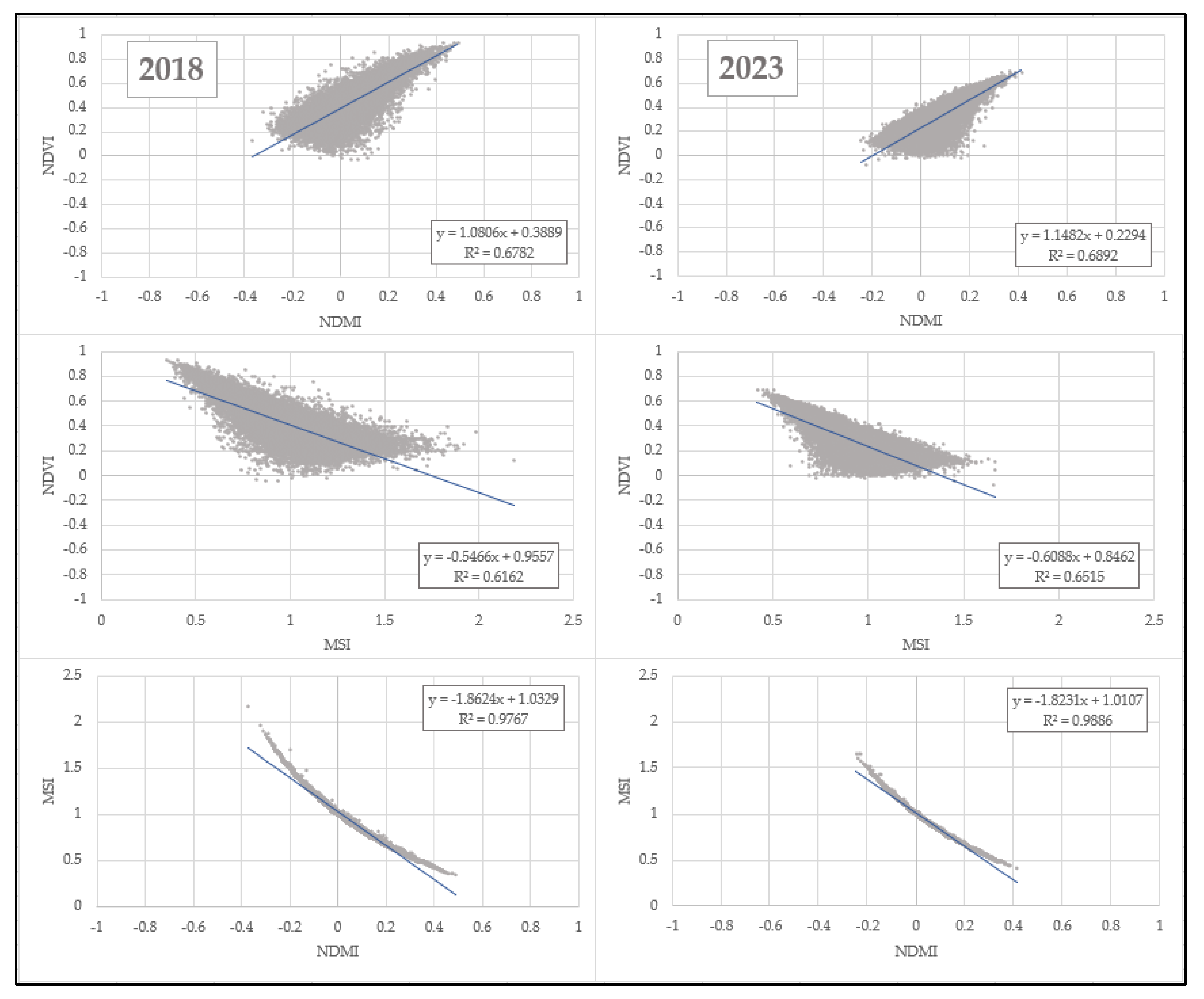
| NDVI | GNDVI | GCI | NDWI | NDMI | MSI | NDDI | |||||||||||
|---|---|---|---|---|---|---|---|---|---|---|---|---|---|---|---|---|---|
| NDVI | Pearson's r | — | |||||||||||||||
| p-value | — | ||||||||||||||||
| GNDVI | Pearson's r | 0.979 | *** | — | |||||||||||||
| p-value | < .001 | — | |||||||||||||||
| GCI | Pearson's r | 0.921 | *** | 0.928 | *** | — | |||||||||||
| p-value | < .001 | < .001 | — | ||||||||||||||
| NDWI | Pearson's r | 0.824 | *** | 0.743 | *** | 0.772 | *** | — | |||||||||
| p-value | < .001 | < .001 | < .001 | — | |||||||||||||
| NDMI | Pearson's r | 0.824 | *** | 0.743 | *** | 0.772 | *** | 1.000 | *** | — | |||||||
| p-value | < .001 | < .001 | < .001 | < .001 | — | ||||||||||||
| MSI | Pearson's r | -0.785 | *** | -0.698 | *** | -0.706 | *** | -0.988 | *** | -0.988 | *** | — | |||||
| p-value | < .001 | < .001 | < .001 | < .001 | < .001 | — | |||||||||||
| NDDI | Pearson's r | -0.016 | * | -0.016 | * | -0.011 | -0.012 | -0.012 | 0.012 | — | |||||||
| p-value | 0.014 | 0.012 | 0.075 | 0.056 | 0.056 | 0.069 | — | ||||||||||
| Component | ||||
|---|---|---|---|---|
| 1 | 2 | 3 | Uniqueness | |
| MSI | -0.921 | 0.00722 | ||
| NDMI | 0.891 | 0.00224 | ||
| NDWI | 0.891 | 0.00224 | ||
| GNDVI | 0.917 | 0.01958 | ||
| GCI | 0.875 | 0.06121 | ||
| NDVI | 0.495 | 0.855 | 0.02425 | |
| NDDI | 1.000 | 1.34e-6 | ||
| Final cluster | NDVI | NDMI | MSI | Description |
|---|---|---|---|---|
| 0 | 1 | 1—2 | 1—5 | uncultivated area/young crop |
| 1 | 4—5 | 2 | 1 | irrigated high cover crop |
| 2 | 2—3 | 2 | 1 | irrigated low cover crop |
| 3 | 4—5 | 2 | 2—4 | irrigated water-stressed high cover crops |
| 4 | 2—3 | 2 | 2—4 | irrigated water-stressed low cover crops |
| 5 | 4—5 | 1 | 2—4 | non-irrigated water-stressed high cover crop |
| 6 | 2—3 | 1 | 2—4 | non-irrigated water-stressed low cover crop |
| Cluster description | 2018 ha |
% |
2023 ha |
% |
|---|---|---|---|---|
| Uncultivated área/young crop | 450.90 | 3.53 | 1,998.47 | 13.90 |
| Irrigated high cover crop | 5,817.10 | 45.50 | 2,523.06 | 17.55 |
| Irrigated low cover crop | 801.35 | 6.27 | 3,530.44 | 24.56 |
| Irrigated water-stressed high cover crop | 539.08 | 4.22 | 8.37 | 0.06 |
| Irrigated water-stressed low cover crop | 829.16 | 6.49 | 2,524.14 | 17.56 |
| Non-irrigated water-stressed high cover crop | 451.31 | 3.53 | 0.09 | 0.001 |
| Non-irrigated water-stressed low cover crop | 3,896.45 | 30.48 | 3,788.00 | 26.36 |
| Total | 12,785.35 | 100 | 14,372.56 | 100 |
| CHANGES | 2018 | 2023 | change ha | change % |
|---|---|---|---|---|
| 1 | unchanged | unchanged | 5,349.77 | 37.22 |
| 2 | non-irrigated water-stressed low cover crop | uncultivated area | 3,008.36 | 20.93 |
| 3 | irrigated high cover crop | irrigated low cover crop | 1,960.13 | 13.64 |
| 4 | non-irrigated water-stressed low cover crop | irrigated water-stressed low cover crop | 1,087.28 | 7.56 |
| 5 | non-irrigated water-stressed low cover crop | irrigated low cover crop | 812.44 | 5.65 |
| 6 | irrigated high cover crop | irrigated water-stressed low cover crop | 521.40 | 3.63 |
| 7 | irrigated high cover crop | non-irrigated water-stressed low cover crop | 454.68 | 3.16 |
| 8 | irrigated water-stressed low cover crop | irrigated low cover crop | 432.24 | 3.01 |
| 9 | non-irrigated water-stressed high cover crop | irrigated low cover crop | 259.65 | 1.81 |
| 10 | non-irrigated water-stressed high cover crop | non-irrigated water-stressed low cover crop | 252.95 | 1.76 |
| 11 | irrigated low cover crop | irrigated water-stressed low cover crop | 233.66 | 1.63 |
| Total | 14,372.56 | 100 |
Disclaimer/Publisher’s Note: The statements, opinions and data contained in all publications are solely those of the individual author(s) and contributor(s) and not of MDPI and/or the editor(s). MDPI and/or the editor(s) disclaim responsibility for any injury to people or property resulting from any ideas, methods, instructions or products referred to in the content. |
© 2025 by the authors. Licensee MDPI, Basel, Switzerland. This article is an open access article distributed under the terms and conditions of the Creative Commons Attribution (CC BY) license (http://creativecommons.org/licenses/by/4.0/).


