
Submitted:
27 June 2025
Posted:
01 July 2025
You are already at the latest version
Abstract
Droughts significantly impact agriculture, water resources, and ecosystems. Their timely detection is essential for implementing effective mitigation strategies. This study explores the use of multispectral Sentinel-2 remote sensing indices and machine learning techniques to detect drought conditions in three distinct regions of India such as Jodhpur, Amravati, and Thanjavur during the Rabi season (October-April). Twelve remote sensing indices were studied to assess different aspects of vegetation health, soil moisture, and water stress, and their possible joint use and influence as indicators of regional drought events. Reference data used to define drought conditions in each region was primarily sourced from official government drought declarations, and regional and national news publications, which provide seasonal maps of drought conditions across the country. Based on this information, a District vs. Year (3×6) Ground truth is created, indicating the presence or absence of drought (Yes/No) for each region across the six-year period. Using this ground truth table, we extended the remote sensing dataset by adding a binary drought label for each observation: 1 for “Drought” and 0 for “No Drought”. The dataset is organized by year (2016–2021) in a two-dimensional format, with indices as columns and observations as rows. Each observation represents a single measurement of the remote sensing indices. This enriched dataset serves as the foundation for training and evaluating machine learning models aimed at classifying drought conditions based on spectral information. The resultant remote sensing dataset was used to predict drought events through various machine learning models, including Random Forest, XGBoost, Bagging Classifier, and Gradient Boosting. Among the models, the Bagging Classifier achieved the highest accuracy (84.15%), followed closely by Random Forest (83.39%) and XGBoost (82.30%). In terms of precision, Random Forest and Bagging Classifier performed comparably (83.49% and 83.44% respectively), while XGBoost achieved a precision of 79.82%. We applied a seasonal majority-voting strategy, assigning a final drought label for each region and Rabi season based on the majority of predicted monthly labels. Using this method, XGBoost, Random Forest, and Bagging Classifier achieved 94% accuracy, precision, and recall, while Gradient Boosting reached 83% across all metrics. The SHapley Additive exPlanations (SHAP) analysis revealed that Normalized Multi-band Drought Index (NMDI) and Day of the Season (DOS) consistently emerged as the most influential feature in determining model predictions. This finding is supported by the Borda Count and weighted sum analysis, which ranked NMDI, and DOS as the top feature across all models. Additionally, Red-edge Chlorophyll Index (RECI), Enhanced vegetation index (EVI), Normalized Difference Moisture Index (NDMI), and Ratio Drought Index (RDI) were identified as important features contributing to model performance. These features provide valuable insights into the underlying patterns and relationships within the data. To evaluate the impact of feature selection, we further conducted a feature ablation study. We trained each model using different combinations of top features: Top 1, Top 2, Top 3, Top 4, and Top 5. The performance of each model was assessed based on accuracy, precision, and recall. XGBoost demonstrated the best overall performance, especially when using the top 5 features.
Keywords:
Copernicus
; Agricultural Applications
; Sentinel-2
; SHAP
; Drought Detection
; Borda Count
; XGBoost
; India
; Machine Learning
; Remote Sensing Indices
; Bagging Classifier)
1. Introduction
Droughts are climatic events that occur naturally and play a significant role in shaping ecosystems by influencing species adaptation, water availability, and vegetation dynamics. However, despite their ecological importance, droughts frequently lead to severe consequences for human populations, including widespread suffering, loss of livelihoods, and adverse environmental and economic impacts [1]. These effects are particularly pronounced in the agricultural sector, where reduced water availability and declining soil moisture levels directly threaten crop yields and food security. Naturally, droughts pose a significant threat to India’s agricultural sector, which is highly sensitive to variations in rainfall and water availability. Effective drought monitoring is critical for ensuring food security and minimizing economic losses, particularly in a country where agriculture supports a substantial portion of the population. The principal cause of drought is the deficit of precipitation [2]. Droughts can be categorized based on different factors such as meteorological - deficit in precipitation, hydrological - deficit in groundwater, or total water storage, agricultural - deficit in soil moisture, and socioeconomic - impact of drought conditions on socioeconomic goods [3]. All these aspects are highly correlated. A significant decline in soil moisture levels compared to normal conditions can be characterized by the transition from meteorological drought to agricultural drought [4]. Further prolonged deficit in soil moisture may lead to hydrological drought [4]. Agricultural drought, in turn, has both direct and indirect impacts on food-related industries, ultimately weakening the overall economy of a country [5]. India is an agrarian country with a diverse climate and socio-economical structure. Different parts of India have endured multiple agricultural droughts lasting between 5 and 17 years, leading to severe famine and widespread loss of human and livestock populations in the last hundred years [5]. Given India’s vast and varied agricultural landscapes, accurately assessing drought conditions remains a significant challenge. The country’s diverse climatic conditions, ranging from arid and semi-arid zones to tropical and subtropical regions, influence the frequency and intensity of droughts. Additionally, varying cropping patterns across different agro-climatic zones further complicate drought monitoring efforts. The lack of comprehensive, consolidated ground truth data for validation adds another layer of complexity, making it difficult to establish reliable drought assessment models. Addressing these challenges requires analyzing drought conditions through different modalities such as satellite-based remote sensing, climate modeling, and on-ground observations to enhance drought detection and monitoring across India’s agricultural sector.
1.1. Related Work
Several studies have employed a variety of approaches for drought detection and monitoring, utilizing different methodologies such as remote sensing, climate modeling, hydrological analysis, and ground-based observations to assess drought conditions across various spatial and temporal scales. Different remote sensing technologies such as multispectral, thermal infrared, and microwave data are widely employed to retrieve key drought indicators such as precipitation [6], soil moisture [3], and evaporation [7]. Insufficient precipitation can significantly impact plant health by reducing photosynthetic capacity [3]. When water availability decreases, plants experience physiological stress, which results into lower photosynthetic activity. This reduction affects the absorption of solar radiation in photosynthetically active wavelengths, such as visible and near-infrared. Thus, vegetation may exhibit changes in spectral reflectance, which can be detected through remote sensing techniques [3]. Therefore, drought detection and monitoring have been increasingly conducted using multiple indicators derived from satellite imagery. Normalized difference vegetation index (NDVI) has been proven to be an effective indicator of vegetation stress, however, it may not provide the underlying cause of the stress which may relate to different factors such as plant disease, flood, and others [8]. Hence, NDVI or vegetation indices along with other indices such as land surface temperate [9] are applied for drought monitoring. Short-wave infra-red bands are also found to be susceptible to soil moisture and leaf water content [3]. Thus, Normalized difference water index (NDWI), and combinations of NDWI, and NDVI are studied to detect drought monitoring [10]. Different climate-based indices, biophysical parameters along with vegetation conditions are used to form an index named Vegetation Drought Response Index [11]. However, it is complex to compute and its performance varies widely in different regions [11]. Several indices are proposed for the identification and monitoring of plant stress and subsequently drought such as Crop Water Stress Index (CWSI) [12], Water Deficit Index (WDI) [13], Evaporative Stress Index (ESI) [14], Drought Severity Index (DSI) [15], and several others [3]. Multivariate drought indices are typically based on four factors such as vegetation health, soil moisture levels, hydroclimatic variables, and crop stress status [5]. One such combined drought index using hydro-climatic and biophysical variables which indicate anomalies in soil moisture conditions, rainfall, and crop-sown area progression, is proposed using synthetic aperture radar (SAR) images of Sentinel for monitoring early-season agricultural drought in South Asia [16]. A regional agricultural drought index (RegCDI) based on crop water stress, soil moisture deficits, and vegetation health is used in the detection of a regional drought of India [5]. Such indices have been proven insightful in various circumstances. However, traditional drought indices based assessments often struggle to adapt across diverse environmental conditions, which may lead to inconsistencies in detection and prediction. As an example, NDVI have certain limitations in detecting early-season drought for reduced sensitivity to fluctuations in soil moisture, and a delayed response to rainfall variations [16]. The challenges associated with generalization and sensitivity to various atmospheric and climatic factors create an opportunity for the application of machine learning in drought monitoring. With their ability to analyze complex, non-linear relationships, machine learning techniques offer a promising approach to enhance the accuracy and robustness of drought monitoring by integrating multiple data sources, adjusting for regional variations, and improving predictive capabilities.
Sentinel-2 has been found instrumental to detect the drought related land surface changes [17,18]. However, the lack of thermal bands in Sentinel-2 and its limited direct applicability for drought monitoring impose certain constraints on its effectiveness [18]. These limitations can hinder the satellite’s ability to provide comprehensive data for drought analysis, as thermal information is crucial for assessing parameters like soil moisture and evapotranspiration. Nevertheless, these challenges are addressed through multi-modal analysis, which integrates data from multiple sources or sensors. Fusion of Landsat 8 and Sentinel 2 data has provided a significant leap in drought analysis, particularly by perpendicular drought index [19]. In [1], a multi-modal analysis is conducted by integrating radar-based surface moisture estimation and multi-spectral vegetation indices derived from Sentinel-1, Sentinel-2, and Landsat-8 imagery for the savanna ecosystem in South Africa. SAR imagery has proven to be highly effective in regions with persistent cloud cover. However, a major limitation of using SAR for drought assessment is the need to accurately parameterize surface roughness [16]. Nonetheless, the added complexity of multi-modal drought detection is hindered by two key challenges: the intricate processing required for SAR images and the discrepancy in spatial resolution when integrating Sentinel 2 data with other multi-spectral satellites like Landsat 8. These factors can complicate the analysis and limit the effectiveness of combining such datasets for drought monitoring. On the other hand, vegetation indices derived from Sentinel-2, such as NDVI and others, have demonstrated a stronger correlation with drought conditions and have yielded more reliable outcomes, as highlighted in recent studies [18]. Hence, this paper focuses on utilizing Sentinel-2-derived indices and harnessing the power of machine learning to enhance the accuracy and reliability of drought detection. The prolonged impact of drought can lead to substantial changes in land use and land cover (LULC). Machine learning techniques are conducted in the literature through a spatio-temporal analysis on land use and land cover (LULC), to effectively detect drought and visualize its transformative effects over time [18,20]. The focus area of this work is the agricultural regions in different parts of India. The high spatial resolution of Sentinel-2, ranging from meters, is well-suited for monitoring small-scale field crops, which are prevalent across India [21].
Multiple linear regression (MLR), long short-term memory (LSTM), and random forest (RF) have been employed to detect flash drought in China [22]. Random forest (RF) has been found most effective among different machine learning algorithms in drought stress detection of wheat [23]. Four machine learning models of RF, the Extreme Gradient Boost (XGB), the Convolutional neural network (CNN) and the Long-term short memory (LSTM) are used for the estimation of meteorological drought in [24]. In [25], the naive bayes classifier has been found better suitable than decision trees to characterize droughts. A deep neural network was employed in [26] to estimate soil moisture for agricultural drought monitoring in South Korea. In [27], three advanced machine learning techniques, bias-corrected random forest, support vector machine (SVM), and multi-layer perceptron neural network were employed to detect and analyze agricultural drought in South-Eastern Australia. It is observed that machine learning techniques are widely used in recent paradigms in monitoring and forecasting of meteorological, hydrological and agricultural droughts [28]. Still, application of machine learning techniques in different climatic conditions of India through multiple spectral and temporal indices to detect drought with high accuracy is under-explored. A significant research gap is too observed in the literature in quantifying the influence of different spectral and temporal parameters on detecting drought in different climatic locations of India. This work contributes to addressing these gaps by evaluating the potential of a range of indexes based on Sentinel-2 data toward drought detection in India with higher accuracy. Sentinel-2 offers open multispectral and multitemporal data under the Copernicus open access scheme. These data are well-suited for detecting agricultural drought indicators such as vegetation health and water stress. By leveraging key indices from Sentinel-2 (S-2) data, we aim to develop a scalable drought detection system tailored to India’s diverse regions. In our experiments, we focused on three districts, i.e. Jodhpur(Rajasthan), Amravati(Maharashtra), and Thanjavur(Tamil Nadu), which experience distinct climatic conditions and cultivate different crops, enabling a comprehensive evaluation of drought detection during the critical Rabi season. To enhance the reliability and interpretability of the machine learning models, SHAP (SHapley Additive exPlanations) [29] analysis is employed to determine the weight and importance of individual features. For aggregating outputs from multiple models, Borda Count method[30] and Weighted Sum approach are further utilized to identify the top features that most closely relate to drought conditions. Furthermore, the top-ranked features, from the first to the fifth, are systematically evaluated to analyze their individual and collective performance trends across the study regions. This approach not only addresses an important challenge posed on India’s diverse agricultural landscapes, but also provides relevant clues for identifying and prioritizing the factors driving drought conditions, paving the way for more targeted and effective drought mitigation strategies.
2. Preliminaries
A few established techniques are used in this work, described below for the readers’ convenience.
2.1. Remote Sensing Indexes
Multispectral images widely use spectral indices to enhance and identify specific spectral features of a relevant land cover class. The spectral indices used in this work are briefly described below, with the rationale for including each of them in a drought identification study.
2.1.1. Normalized Difference Vegetation Index
The Normalized Difference Vegetation Index (NDVI) is a widely used metric to assess vegetation health using near-infrared (NIR) and red (Red) bands as shown in Equation (1):
NDVI values range between , where higher values denote denser/healthier vegetation. NDVI is easily interpretable and widely applicable. Although it is affected by soil reflectance in sparsely vegetated areas, NDVI performs well also in extreme conditions [31].
2.1.2. Enhanced Vegetation Index
The Enhanced vegetation index (EVI) is regarded as an enhanced version of the NDVI. It provides greater sensitivity in high-biomass regions, thus improving vegetation monitoring capabilities. It achieves this by decoupling the canopy background signal and reducing the impact of atmospheric interference [32]. It is demonstrated in [33] that EVI can be effectively used to monitor water stress. EVI showed indeed high correlation with patch pressure (Pp), a measure of leaf water status [33]. Moreover, EVI is sensitive to changes in plant water status hence it can detect temporary changes in leaf hydration. It values between [34], and it is computed using Red, NIR, and Blue bands as per Equation (2):
2.1.3. Atmospherically Resistant Vegetation Index
The Atmospherically Resistant Vegetation Index (ARVI) is an effective tool to mitigate the effect of high atmospheric aerosol content [35] when evaluating vegetation status. ARVI is computed as shown in Equation (3):
Here, y is a coefficient tuned to compensate the effects of atmospheric aerosols, estimated through relative values of red and blue bands [35]. Simulations show that, while ARVI features a dynamic range similar to NDVI, it is four times less sensitive to atmospheric effects than NDVI [36]. A self-correction process on the red channel is employed in ARVI to achieve this robustness [37].
2.1.4. Normalized Difference Water Index
The Normalized Difference Water Index (NDWI), which is primarily a water body index, can also be utilized to monitor drought stress in agricultural areas, providing timely information on crop quality and development [38]. It is particularly valuable for precision agriculture and forest health monitoring, as it is sensitive to changes in plant water content, which is insightful for drought detection in various vegetation types [38]. It ranges between [39] as visible from Equation (4):
2.1.5. Soil-Adjusted Vegetation Index
The Soil-Adjusted Vegetation Index (SAVI) introduces a soil brightness correction factor (L) to mitigate the soil reflectance factor in vegetation indices [40] as shown in Equation (5). It demonstrates superior stability in time series analysis of vegetation [41]. Hence, SAVI can be found invaluable for drought detection particularly in areas where soil background might bias other vegetation indices [41].
2.1.6. Transformed Vegetative Index
2.1.7. Normalized Difference Moisture Index
The Normalized Difference Moisture Index (NDMI) is a dynamic indicator that characterizes the moisture content of vegetation, making it valuable for drought detection [44]. It has a close correlation with NDVI and effectively tracks changes in vegetation health related to water stress, providing insights into drought conditions in urban and natural environments [45]. It utilizes the short wave infra-red one (SWIR-I) band along with NIR bands as shown in Equation (7):
2.1.8. Normalized Multi-Band Drought Index
The Normalized Multi-band Drought Index (NMDI) demonstrated enhanced sensitivity to drought severity by integrating data from NIR and two short-wave infrared bands (SWIR-I and SWIR-II) [46]; it was found to be effective in estimating both soil and vegetation moisture content. It is computed as shown in Equation (8).
2.1.9. Modified Normalized Water Index
2.1.10. Modified Normalized Difference Vegetation Index
Modified Normalized Difference Vegetation Index (MNDVI) utilizes the mid infra-red (MIR) band [49]. As it can accurately capture changes in vegetation photosynthetic activity, which is often impacted by water availability [49] (Equation (10)), it can provide deeper understanding of the drought conditions:
2.1.11. Ratio Drought Index
2.1.12. Red-Edge Chlorophyll Index
2.2. Machine Learning Classifier
The machine learning models used to classify droughts in this work are Random Forest (RF), Bagging (BGN), Gradient Boost (GB), and XGBoost (XGB). These models are well-suited for remote sensing applications due to their ability to handle complex interactions among variables and to provide a good basis for feature importance analysis. [53,54].
2.3. Random Forest
Random Forest is an ensemble learning algorithm through bagging technique that creates a large number of decision trees [55]. Each tree is trained on a random subset of the data and a random subset of the features. The final prediction is made by aggregating the predictions of individual trees, typically through a majority vote. Random Forests are known for their robustness to overfitting, high accuracy, and ability to handle high-dimensional data [55].
2.3.1. Gradient Boosting Classifier
Gradient Boosting is also an ensemble learning algorithm using the boosting technique to form trees sequentially, with each new tree attempting to correct mistakes made in preceding trees [56]. It aims to minimize a loss function through iteratively adding new trees specifically trained to predict the negative gradient of the loss function. The technique is highly robust and a powerful as it can work with different loss functions.
2.4. Extreme Gradient Boosting (XGBoost)
XGBoost enhances the gradient boosting algorithm with high efficiency and performance [57]. XGBoost algorithm, which is too a boosting technique, creates trees sequentially, with each tree fixing its predecessor’s mistakes. It integrates a regularization objective function with a penalty for model complexity, and thus avoids overfitting. XGBoost often outperforms traditional Gradient Boosting due to its regularization and optimization techniques.
2.4.1. Bagging Classifier
Bagging is an ensemble learning technique that aggregates a variety of models in an attempt to make a prediction with increased accuracy [58]. In bagging (BGN), subsets of training data are generated through bootstrapping. For each subset, a model is constructed, and a prediction is derived through aggregation of model output, in many cases through voting for classification, for a prediction in a classification problem. Bagging reduces variance effectively and helps in overcoming overfitting, especially in complex models.
3. Feature Ranking and Aggregation Techniques
This work also aims at assessing the influence of different features; in the following, a brief description is provided of a few feature ranking and aggregation techniques used in this work.
3.0.2. SHapley Additive exPlanations Analysis
SHapley Additive exPlanations (SHAP) values offer a game-theoretic approach to explain the output of a machine learning model [59,60]. It computes the contribution of each player, i.e. each feature, for the outcome of a game, i.e. the prediction. Formally, the SHAP value for feature i in instance x is calculated as:
Here F, S, and are defined as the set of all features, a subset of features, and the model’s prediction using only the features in S, respectively. It computes the average change in the model’s output when feature i is added to all possible subsets of other features [60,61]. SHAP values can be used for both global and local feature importance analysis. Global importance can be determined by aggregating the absolute SHAP values for all instances. A key advantage of SHAP is its ability to provide both magnitude and direction (positive or negative) of feature influence on the model’s output.
3.0.3. Borda Count
The Borda Count is a voting mechanism designed to aggregate preferences from multiple voters [62]. Each voter ranks the candidates i.e. features, in order of their preferences. For a group of n candidates, a voter assigns points to their most preferred candidate, to their second, and continues in a similar fashion to 0 for the least preferred feature. Next, each candidate’s overall score is computed by adding together all of the points received from all voters. The winner is then determined to be the one with the largest overall score. In feature ranking, the voters can be considered different evaluation metrics or different runs of a feature selection algorithm. The Borda Count aggregates these rankings to produce a consensus [62].
3.0.4. Weighted Sum
The weighted sum method combines multiple feature importance scores or rankings [63]. Given a set of n features and m different importance scores or rankings for each feature, a weight is assigned to each of the m scores, where . The combined score for feature i is then calculated as shown in Equation (14).
is the rank or score of feature i according to the criterion. determines the final influence of each features. The weights () reflect the relative importance of the different criteria. This technique is simple to implement and interpret, however the selection of weights can significantly impact the final ranking. Appropriate weight selection is crucial and often depends on the specific application and the nature of the input scores.
4. Resampling Techniques
This section discusses the resampling techniques employed in this study to address potential class imbalance in the drought data.
4.1. Synthetic Minority Over-Sampling Technique
Synthetic Minority Over-sampling Technique (SMOTE) denotes an oversampling technique that generates synthetic instances for the minority class through its k-nearest neighbors [64]. Synthetic samples are produced over the connecting line segments between the selected instance and its neighbors. This helps in attaining a balanced distribution of classes, and as a consequence, it improves the performance of machine learning algorithms with imbalanced datasets. It addresses the issue of simply duplicating minority class instances, which may lead to overfitting.
4.2. Borderline SMOTE
Borderline SMOTE enhances traditional SMOTE, with a focus placed on generating synthetic samples near the borderline cases of the minority class [65]. This aims at sharpening the decision boundary and, in turn, enhancing classifiers’ effectiveness.
4.3. Adaptive Synthetic Sampling Approach
Adaptive Synthetic Sampling Approach (ADASYN) is an oversampling technique that adaptively generates synthetic samples for the minority class based on the density of neighboring majority class instances [66]. The algorithm prioritizes on generating more synthetic samples in regions where the minority class is harder to learn i.e., surrounded by more majority class instances. This is particularly beneficial when the minority class is sparsely distributed or when there are notable differences in the density of the majority and minority classes.
5. Data and Study Area
Three districts in India were selected as our study area: Jodhpur in Rajasthan state, Amravati in Maharashtra state, and Thanjavur in Tamil Nadu state as shown in Figure 1. These districts feature distinct climates, different agricultural practices, and slightly varying cropping seasons. Each district typically follows two annual cropping cycles: the Kharif (monsoon) season, with sowing in June-July and harvesting in September-October, and the Rabi (winter) season, with sowing in October and harvesting in March-April. We focused exclusively on the Rabi season, as optical satellite data from the Kharif season is often unreliable due to frequent and persistent cloud cover. Sentinel-2 is considered here to collect time series data for 12 remote sensing indices across the three districts from year 2016 to year 2021 through the Google Earth Engine (GEE) cloud infrastructure. Data are selected with cloud cover, covering the period from October 1 of one year to April 30 of the next year. As an example, year “2017” indicates the duration from Oct 2016 to Mar 2017. A drought season is defined as the period spanning from October of the previous year to April of the current year, with each temporal sample labeled as a drought sample. Thus, the number of data points in each year is different, as cloud cover discards a varying number of data points over the years. The initial plan was to employ Level-2A product data for the proposed research. However, before March 2018, Level-2A products were not systematically available from ESA. Users need to generate them locally using tools like the Sen2Cor processor. In March 2018, ESA started the systematic production of Level-2A data. Since our study period spans from October 2016 to April 2021, data covering this entire timeframe is required. Hence, Sentinel-2 Level-1C top-of-atmosphere reflectance data was used instead. This data is acquired for each year (2016-2021) using the “COPERNICUS/S2” image collection in GEE. The collection was filtered by date and cloud cover (). The cloud masking function was applied to each image using the band. District boundaries for Jodhpur, Amravati, and Thanjavur were defined as regions of interest (ROIs) within GEE using the FAO GAUL dataset [67]. Administrative level 2 (ADM2) boundaries are primarily used here. In order to concentrate on agricultural areas, another land cover mask was generated using agricultural land classes from the Copernicus Global Land Cover dataset [68]. The mask was clipped to each district’s boundary to isolate agricultural land within each ROI.
We organized the data by year () in a two-dimensional format. One example is shown in Table 1, with indices as columns and observations as rows. Note that there can be multiple observations recorded on the same day in this dataset, each representing a single measurement of the remote sensing indices. The dataset comprises a total of 13 features per row: 12 spectral indices and a temporal “Day of Season” (DOS) feature, starting from 1 on 1st Oct, this is processed later in preprocessing stage using the date column. The DOS feature conveys information about the time of the year, i.e. it relates other variables to the advancement of the season. The rows span all selected cloud-free days in the mentioned time period for each year and district, creating a comprehensive temporal record for analysis. These rows serve as individual data points for model training and testing, linking the observed remote sensing patterns to drought outcomes. Each value in this row reflects the mean value of a specific index (e.g., NDVI) for an entire district (e.g., Thanjavur) on a particular date at a particular time.
5.1. Drought Declaration Process in India
In India, drought declarations follow a formal, multitiered process outlined in the national Drought Manual [69,70] as shown in Figure 2. This manual was created in 2016 and again revised in 2020. This process begins with routine monitoring of agro-meteorological indicators by specialized agencies: the India Meteorological Department (IMD) analyzes rainfall and temperature data, the National Remote Sensing Centre (NRSC) provides satellite-derived soil moisture and vegetation indices, and the Central Research Institute for Dryland Agriculture (CRIDA) offers agronomic assessments[71]. District-level drought committees, typically chaired by the District Collector with members of agriculture and finance departments, further review these data against predefined criteria (for example, specified rainfall deficits or Standardized Precipitation Index thresholds). When these quantitative triggers are met, field verification teams are deployed to inspect crop conditions and local water availability. The findings of the committees (including any field reports) are submitted to the State government for review. If the state agrees that a district meets the drought criteria, it issues a formal declaration for the affected districts, usually by notification in the State Gazette. In severe cases, the State can also request central relief assistance or activate national contingency plans for drought relief.
Assembling a consolidated ground truth for drought declarations is extremely challenging given the process’s decentralized, multi-tiered nature. Each state (and often each district within it) follows its own procedure and publishes drought notifications in various formats and languages (for example, in State gazettes, local newspapers, or agriculture department bulletins), with no single central repository. Researchers must therefore compile data from many scattered sources. Declarations often rely on qualitative field reports rather than uniform quantitative metrics, and different states may apply different rainfall deficit or SPI thresholds. This heterogeneity makes retrospective interpretation difficult. It is also difficult to confirm that a district did not experience drought, as the absence of an official declaration is not explicitly recorded. Timing adds further complexity: some districts may declare drought only after significant delay or at subdistrict levels, creating inconsistencies between district-wide and local reports. Together, these factors make it extremely challenging to build an accurate and unified ground truth data set of drought occurrences; still, even with some difficulties it was possible to assemble a reference dataset as reported in the following subsection.
5.2. Ground Truth Table
The ground truth data was prepared primarily based on meteorological reports, government declarations, and relevant news articles covering regional drought impacts. Table 2 presents an annual summary of drought occurrences in the rabi season in the districts of 2016 to 2021. Consolidating all of this data into a tabular form for better interpretation and future use is one of the contributions of the proposed work. The label “Yes” in Table 2 indicates that a drought was recorded in the corresponding year for a district for the rabi season, while “No” denotes the absence of drought conditions. For example, severe drought was widespread in different regions in 2016 and 2019, affecting agricultural productivity and water resources. However, in other years, some districts have experienced drought, while others have not. The table captures these regional patterns in drought frequency over the six-year period.
An additional column representing the drought label was added in order to enable the application of machine learning techniques. This label was derived from the consolidated ground truth data presented in Table 1, which indicates whether a drought occurred during the Rabi season for that particular district and year. In particular, for every observation in the dataset, we assigned a binary drought label: “Drought” encoded as 1 and “No Drought” encoded as 0. For example, since a drought was reported in Jodhpur during the 2016 rabi season, all corresponding observations for Jodhpur in 2016 were labeled with 1. This practice guarantee that each row in the dataset not only captures the temporal and spectral characteristics of the season but also carries the correct drought classification, rendering it suitable to use in training and evaluating supervised machine learning models.
We assign a positive drought label to a (district, year, season) entry only if all three identifiers are identical and the occurrence is corroborated by at least two independent and reliable sources. These sources include formal government declarations bulletins —such as state-level drought notifications or central advisories—quantitative meteorological indicators like severely negative SPI values or significant rainfall deviations, and credible public documentation such as state gazette publications, Parliament Q&A transcripts, or regionally verified news reports. All these sources should specifically to the same district and Rabi season to qualify. Entries lacking such corroboration are either labeled as non-drought or excluded if the evidence is inconclusive. This rigorous, cross-validated labelling framework enhances the reliability of the dataset and ensures its suitability for training and validating supervised machine learning models aimed at drought prediction.
5.2.1. Jodhpur
In the Rabi season of 2016, Rajasthan faced severe drought conditions, with 19 out of 33 districts being officially declared drought-affected. The Hindu newspaper reported that the state grappled with a serious water crisis, prompting the government to deploy water trains to parched Bhilwara and water tankers to other regions [72]. Districts such as Ajmer, Banswara, Baran, Barmer, Bhilwara, Chittorgarh, Churu, Dungarpur, Hanumangarh, Jaipur, Jaisalmer, Jalore, Jhunjhunu, Jodhpur, Nagaur, Pali, Rajsamand, Udaipur, and Pratapgarh were the most affected. A follow-up report by [73] also confirmed that Rajasthan was among 11 drought-affected states during 2015-16. Furthermore, a parliamentary document corroborated the declaration and listed Rajasthan’s drought-affected status during the Rabi season [74].
In 2017, no conclusive evidence was found to support a drought declaration for the Jodhpur district or other parts of Rajasthan. On the contrary, there was positive news of increased agricultural production throughout the state. Additionally, official records from the Parliament [74] confirm that no funds were allocated for drought relief for either the Kharif or Rabi crops in Rajasthan during 2017, further indicating a relatively stable agricultural season. From the same document, it can be seen that the funds were only allocated for the Kharif season of 2018.
In the Rabi season of 2019, there is substantial evidence that the Rajasthan government declared drought before the start of summer. According to [75], more than 5,000 villages across nine districts, including Barmer, Churu, Pali, Bikaner, Jaisalmer, Jalore, Jodhpur, Hanumangarh, and Nagaur, were declared drought-affected by the state government. This severe drought badly hit the region, causing a decline in employment opportunities. Another source in [76] also confirms this news, the government officially declared 5,555 villages as drought-affected, an indication of the intensity of the adverse situation.
In the Rabi season 2020, official notifications confirm that the Government of Rajasthan declared 1,388 villages across 13 tehsils in four districts - Barmer, Jaisalmer, Jodhpur and Hanumangarh - as drought-affected. According to a report by [77], the notification, issued on November 11, 2019, classified 13 villages in Jodhpur district as "severely drought-prone" and 297 villages as "moderately drought-prone." Furthermore, as confirmed by [78], the provisions regarding the drought declaration would remain in force for six months from the date of notification, covering the Rabi season. The central assistance disbursed for drought relief during this period. As per official documentation [79], financial aid was allocated to drought-affected regions, confirming the severe impact of drought on agriculture and livelihoods during this season. However, in contrast, for the Rabi season 2021, no drought declaration was made in Jodhpur district, as documented in the same official record [79].
5.2.2. Amravati
During the Rabi season of 2016 [80], the Maharashtra government declared drought in more than 29,000 villages of the state. Most of these villages were from the parched Marathwada and Vidarbha regions that include Amravati. The state government stated that in these regions, the anewari (i.e. the proportion of failed crops) was below 50 percent in both Kharif and Rabi seasons. In the Rabi season of 2019, the Amravati district in Maharashtra faced severe drought conditions. On November 1, 2018, the Maharashtra government declared drought in 151 tehsils spread across 26 districts, including Amravati, as part of its drought relief program [81]. The program was in effect for six months from the date of declaration, covering a major part of the Rabi season.
According to the National Centre for Crop Forecasting (NCCF), 180 tehsils were identified as vulnerable based on remote sensing data, groundwater table index, reservoir storage, vegetation index, and deficient rainfall [82]. In Vidarbha, which includes Amravati, drought conditions were particularly severe, with only 425 mm of rainfall received instead of the usual 900 mm. This significantly affected orange flowering (Mrig Bahar) which happens February onwards. By February 2019, the drought had reduced the area under Rabi crop cultivation in Maharashtra by 40%, according to government estimates [83]. This significant drop in agricultural output highlighted the lasting impact of the drought on farmers’ livelihoods and regional agriculture.
5.2.3. Thanjavur
In the Rabi season of 2016, no significant evidence for drought was found in Thanjavur district. However, reports indicate that heavy and continuous rains lashed the delta districts, including Thanjavur, as a low-pressure system intensified over the Bay of Bengal. According to a report dated November 16, 2015, standing samba paddy crops remained submerged in waterlogged fields due to widespread rainfall [84]. Kollidam registered 175.5 mm of rainfall, while Sirkali recorded 172.5 mm during a 24-hour period. Furthermore, Sansad reports on drought-affected states confirm that there was no drought declaration for either the Rabi or Kharif season in 2016 [85]. In the Rabi season of 2017, the Tamil Nadu government declared drought on January 10, 2017, due to the severe impact of the retreating monsoon. According to a report by [86], Tamil Nadu, which relies heavily on the northeast monsoon for its winter crops (Rabi), saw a significant 33 percent drop in winter rice sowing. Nagapattinam, Thiruvarur, and Thanjavur were the worst hit district. A Tamil Nadu government document [87] also supports these claims, detailing the severe deviation in rainfall: the state received only 168.3 mm of rainfall, which was 62 percent below the normal, leaving 21 districts with large deficiencies in rainfall. This poor monsoon was the main cause of a shortfall in crop coverage. As early as January 7, 2017, there were indications that Thanjavur would be declared drought-hit. For the Rabi season of 2018, similar conclusions can be drawn. No drought declaration was issued by the government, as per Sansad reports [85]. Further, report dated November 6, 2017, mentions that Thanjavur and neighboring Tiruvarur districts received heavy rainfall, surpassing even the flood-battered Nagapattinam district during a 24-hour duration [88]. This rainfall likely alleviated drought concerns for the subsequent agricultural seasons. In the Rabi season of 2019, Thanjavur district in Tamil Nadu faced severe drought conditions due to the widespread failure of the Northeast monsoon. According to a report dated March 21, 2019, the Tamil Nadu government declared 24 districts, including Thanjavur, as drought-affected [89]. The failed Northeast monsoon, which normally lasts from October to December, significantly impacted the Rabi crops in Tamil Nadu. During the Rabi season of 2020, reports indicate that the Northeast monsoon continued to bring substantial rainfall to the delta districts, including Thanjavur. A weather forecast from December 12, 2019, predicted heavy rains from December 13 for Thanjavur, Nagapattinam, Tiruvarur, and Pudukottai districts. This followed an already active Northeast monsoon, which brought 14 cm more rainfall than usual [90]. No substantial evidence of drought was found in this season. In the Rabi season of 2021, there were no major indications of drought in Thanjavur. There were observations of heavy rains due to the onset of the Northeast monsoon in October 2020. The Northeast monsoon set in on October 28, 2020, and there was heavy rainfall in South India, which included Thanjavur [91]. Besides this, the Southwest monsoon also contributed heavy rainfall to the area, thereby enhancing the agrarian conditions. Additional confirmation from other reports indicates that the region underwent harsh weather conditions; however, there was no indication of a drought event. Cyclone Nivar, which hit the coastal areas, brought flooding throughout Tamil Nadu, especially in Thanjavur, which also experienced heavy rains [92,93]. While these incidents do not completely eliminate the chances of agricultural drought-like situations, they heavily indicate that the 2021 Rabi season in Thanjavur did not see a drought.
6. Methodology
In this work, drought conditions are identified by different machine learning algorithms in different regions of India based on remote sensing indices. The methodology can be divided into three sections such as data preprocessing, feature engineering, and model training as discussed below.
6.1. Data Acquisition and Preprocessing
First, twelve vegetation and drought indices such as NDVI, EVI, ARVI, NDWI, SAVI, TVI, NDMI, NMDI, MNDWI, MNDVI, RDI, RECI were computed for each image using the appropriate spectral bands. Next, the agricultural land mask, clipped to the district boundary, was applied to each image to retain only data from agricultural areas. Here, data both with and without agricultural land mask are studied. For each image and each index, the mean value within the whole district and the district’s agricultural area were computed. Further, the date of each image acquisition was extracted, and a “Day of the Season” (DOS) feature is created, representing the day number within the Rabi season (October 1st to April 30th). Next, the data rows containing any NaN (Not a Number) or empty values were removed to ensure data quality and prevent issues during model training. Yearly data for each district were concatenated into a single DataFrame. Unnecessary columns, including “system:index” (related to GEE data management) and geolocation data (“.geo”), were removed. A “District” column was added to identify the district. A “Drought” column was added to represent Table 2 contents. The process flow for the preprocessing stage is shown in Figure 3. The resulting time series data for each district and year, consisting of date, “Day of the Season”, and the twelve spectral indices, were further studied for feature engineering as explained below.
6.2. Feature Engineering
Following the data acquisition and initial preprocessing steps described in the previous subsection, the data underwent further processing and feature engineering. The combined data was shuffled randomly to ensure that the training and testing sets were representative of the overall data distribution. The first 12 spectral indices were normalized to a range between 0 and 1. This step is crucial as a significant number of machine learning algorithms are sensitive to feature scaling, such as gradient-based techniques. The DOS, Year, Month, District, and Drought values were not scaled. The data was split into training and testing sets using an split. The methodology considered addressing potential class imbalance using techniques like SMOTE, Borderline SMOTE, or ADASYN. These methods generate synthetic samples for the minority class to balance the dataset.
6.3. Machine Learning Model Training and Evaluation
Four machine learning models were trained and evaluated for drought classification: XGBoost (XGB), Random Forest (RF), Bagging Classifier (BGN), and Gradient Boosting (GB) Classifier. Each model was trained on the training dataset. Hyperparameters for each model (e.g., number of estimators, random state) were empirically determined through experimentation. The trained models were used to predict drought occurrences on the test dataset. The performance of each model was evaluated using accuracy, precision, and recall metrics; precision and recall were calculated with the positive label (drought) designated as class 1. An additional evaluation step was performed to assess the models’ ability to correctly classify drought at the district-year level. The test data was grouped by district and year. For each group, a majority vote was taken based on the individual predictions of a machine learning technique within the group. This majority prediction was then compared to the actual drought label for that district and year. Similarly, the accuracy, precision, and recall of this group-level classification were also computed.
A SHapley Additive exPlanations (SHAP) analysis was performed for each model to understand feature importance and the impact of individual features on model predictions. SHAP summary plots, i.e. bar charts and beeswarm plot both were studied to understand the performance of each features. Borda Count and Weighted Sum were used to aggregate feature importance rankings obtained from SHAP values for XGBoost, Random Forest, and Bagging models, separately. The mean absolute SHAP values are used to represent the feature importance for each model. The Borda Count method and weighted sum method assigned points to features based on their rank in each model’s feature importance list. Two separate lists of the top 5 features were created. A feature with the highest total Borda Count or the weighted sum was considered the most important. The models were further evaluated using only the top-ranked features identified by the Borda Count and weighted sum. The models were trained and tested using the top 1, top 2, top 3, top 4, and top 5 features, and their performance metrics were further analyzed.
Figure 4.
Machine Learning Workflow.

6.4. Error Analysis
Confusion matrix analysis was performed to provide a more detailed understanding of the classification performance of each model. For each model (XGBoost, Random Forest, Bagging Classifier, and Gradient Boosting Classifier), a confusion matrix was generated. The axes of the confusion matrices were labeled to represent the true and predicted classes (No Drought and Drought).
This analysis allowed for a more in-depth examination of the types of errors made by each model, providing insights into their strengths and weaknesses in classifying drought conditions. For example, the confusion matrices can reveal if a model is more prone to false positives (predicting drought when there is none) or false negatives (failing to predict drought when it occurs). This information is valuable for understanding the practical implications of using each model for drought monitoring.
6.5. Software and Libraries
The data processing and machine learning analysis were conducted using Python with different libraries such as: Pandas, NumPy, Scikit-learn, XGBoost, SHAP, and Imbalanced-learn. Matplotlib was used for plotting graphs.
6.6. Evaluation Metrics
All models were evaluated based on the traditional metrics: Accuracy, Precision, and Recall. Drought prediction was treated as the positive (P) class, whereas no drought as the negative (N) class; as per prediction results, , , , and are defined as true positive, false positive, false negative, and true negative cases, respectively. Based on the above definition, the metrics are as follows:
- Accuracy: The percentage of correct predictions. It is defined as .
- Precision: The fraction of true drought predictions among all predicted droughts. It is defined as .
- Recall: The fraction of actual droughts that were correctly identified. It is defined as
7. Results & Discussion
As discussed, Sentinel-2 data with less than cloud cover were utilized for experimentation. Additionally, an “agricultural land” mask was considered, to focus specifically on cropland areas. Different machine learning techniques over 12 remote sensing indices and a temporal data item (DOS, or Day-Of-Season) are applied to distinguish drought and non-drought. Ground truth data on drought conditions (Table 2) was used to define class labels. A drought season is defined as the period spanning from October of the previous year to April of the current year. Consequently, Sentinel-2 data from these periods are used to train the machine learning models.
7.1. Model Performance
Four decision tree based bagging classifiers, such as RF, GB, BGN, and XGB are utilized. It can be observed from Table 2, that the occurrences of drought, i.e. “Yes” labels are less frequent than non-occurrence of drought, i.e. “No” labels. Hence, a data imbalance occurs between drought and non-drought data, which may hamper the performance of the machine learning techniques. Different strategies, primarily oversampling strategies, are applied in this paper to tackle such imbalance. Sentinel images were downloaded based on the considered month of each year, for each selected region. These images with adequate levels were used to train the model.
To assess the impact of oversampling techniques that were implemented to reduce imbalance, performance assessment is divided into two parts: one carried out on results without oversampling and the other after oversampling on the data was implemented, as detailed in the following sections.
7.1.1. Before Oversampling
The accuracy of the machine learning techniques without oversampling is shown in Table 3. Throughout the paper, the terms accuracy, precision, and recall refer to the overall accuracy of the model, the precision of drought detection, and the recall of drought detection, respectively. It can be observed from the Table 3 that the bagging classifier provides overall better performance. RF follows closely in overall accuracy. The precision and recall of RF are also closer to Bagging classifiers. XGBoost performs reasonably well, whereas GB provides the lowest performance. Bagging classifier tends to reduce overfitting and variance. Whereas, XGB may be found susceptible to imbalance data. Further, GB too shows overfitting to majority classes. Hence, the performance of XGB, and GB may be found worse than BGN.
7.1.2. SMOTE
SMOTE randomly generates synthetic minority points by interpolating between existing minority class instances to balance the data. The outcomes of the models after balancing the drought and non-drought data using SMOTE are shown in Table 4. The overall accuracies and precision of drought dropped for all the machine learning models. It indicates that SMOTE may not be fully effective in this context. However, the recalls of the minority class, i.e. detection of drought, have been improved in all the cases. This suggests that SMOTE enhances the detection of drought instances but at the cost of overall performance. Hence, it may require data-aware oversampling. Thus, borderline SMOTE, and ADASYN are further employed.
7.1.3. Borderline SMOTE
Borderline SMOTE focuses on generating synthetic samples near the decision boundary, where misclassification is more likely. It can be observed from Table 5 that the accuracy and precision have been improved in XGB, and RF. The recall of XGB also improved. Hence, the data imbalance was affecting the performance of XGB. However, the improvements are marginal and recall of drought has worsened. As the performance of the models has gone better than SMOTE, this indicates that the classes have complex decision boundaries, making them challenging to separate.
7.1.4. ADASYN
Further, ADASYN is applied for oversampling, as it adaptively generates more synthetic samples for harder-to-learn minority class instances. The overall accuracies for XGB, and RF have been improved. The recalls of drought are better in all the models. However, the precision of drought is lower. It provides a balanced performance of over accuracy in all the classes. Hence, the ADASYN oversampling provides better outcome, proving a complex decision boundary, however, the precision is decreased. Additionally, we conduct an error analysis to gain deeper insights into the models’ performance and identify areas for improvement.

Table 6.
ADASYN: Comparison of classification methods based on Accuracy, Precision, and Recall.
| Methods/Metrics | Accuracy | Precision | Recall |
|---|---|---|---|
| XG Boost | 0.8426 | 0.7859 | 0.8269 |
| Random Forest | 0.8426 | 0.7829 | 0.8324 |
| Bagging Classifier | 0.8328 | 0.7807 | 0.8022 |
| Gradient Boosting | 0.7177 | 0.6176 | 0.7500 |
7.2. Error Analysis
Further, the confusion matrix of BGN, XGB, RF, and GB are shown in Table 7 for the analysis of error. BGN has type-I and type-II error rates of , and . It can be observed that RF provides marginally better type-I and marginally inferior type-II error rates of , and , respectively. The primary objective of this paper is to identify drought conditions; hence, type-II error, i.e. a drought condition detected as non-drought needs to be optimized. Though the overall accuracy of XGB is nominally inferior than RF, however, it provides better type-II error, , than RF (Table 7). This highlights the potential for improved performance of XGB. However, GB provides a very high type-II error, in this case errors in the minority class, of . GB has been found to be susceptible to overfit on the majority class. Therefore, implementing a data balancing strategy can serve as an effective solution. On the other hand, the “Drought” class appears to be harder to predict, as indicated by the higher type-II errors across all models. This suggests that drought conditions may have subtle or complex patterns that are challenging to capture using spectral indices.
The confusion matrices of the machine learning models with SMOTE are shown in Table 8. It can be observed that the type-II error has been reduced in all the classifiers - XGB, RF, BGN, and GB to , , , and , respectively. These improvements show that machine learning techniques, especially GB, were affected by imbalanced dataset and overfitting of majority data. XGB and RF have demonstrated robustness and broad applicability in the literature. Their reduced type-II error rate highlights their effectiveness in learning from the data. In spite of that, type-I error rate has increased in all the cases. SMOTE generates synthetic points randomly. This may imply that many synthetic points are being generated in regions where they do not contribute significantly to improving classification. Therefore, data-aware oversampling techniques, such as Borderline SMOTE and ADASYN, can serve as effective solutions.
Borderline SMOTE, as the name suggests, reinforces the decision boundary by generating synthetic samples only in critical regions, rather than randomly across the feature space like standard SMOTE. This is particularly effective when a significant number of samples of the minority class, i.e. drought data, resides at the decision boundary. It can be observed from Table 9 that type-II error rate has been marginally improved, along with type-I error in all cases. However, type-II error rates in SMOTE were better than Borderline SMOTE. Hence, it can be inferred that while some minority samples exist at the decision boundary, they are not the sole factor affecting performance. Hence, there might be ambiguous regions or complex decision boundaries that affect performance.
ADASYN not only generates synthetic samples near the boundary but also prioritizes harder-to-classify regions. The type-I and type-II error rates in XGB, RF, BGN, and GB are found as , , ,, respectively as shown in Table 10. It can be observed that type-I and type-II error rates have been improved in XGB, RF, and BGN. Therefore, the overall accuracy has also been improved. This provides deeper insight into the data distribution. It can be inferred that these 12 spectral indices along with DOS, the temporal feature, create an overlapping distribution of drought and non-drought classes with complex decision boundaries. It also provides an explanation of the suboptimal performance of GB.
This study focuses on agricultural drought during the Rabi season, with data collected across all phenological phases, from sowing to harvesting. Spectral indices vary throughout these phases, creating complex decision boundaries between drought and non-drought. Since drought is declared on a seasonal basis, detecting it effectively requires considering data across the entire season. However, using only seasonal data would result in a small dataset, unsuitable for machine learning. To address this, a seasonal majority-voting strategy is applied, where individual observations within each Rabi season are aggregated to determine the overall drought condition. This approach balances the need for sufficient data with the ability to capture temporal patterns within the season.
7.3. Model Performance (Season Majority-Voting Strategy)
In the next step, the performance of the machine learning models are studied Rabi season-wise. For a region in a year, i.e. Rabi season, all the predicted labels are computed. The final label is assigned based on the majority vote. The accuracies for season majority-voting strategy are computed without oversampling as shown in Table 11. It can be observed that XGB, RF, and BGN provide accuracy, precision and recall, all of . The small size of the yearly sample pool results into a limited number of values for overall accuracy. Out of the six-year dataset from three different locations, these models incorrectly classify only one instance. The performance of SMOTE through internal voting is shown in Table 12. The performance of SMOTE was worse as shown in Table 8. Thus, though XGB, and BGN provide an accuracy of , the accuracy of RF is dropped to . Borderline SMOTE, and ADASYN performed marginally better. The year-wise performance of Borderline SMOTE, and ADASYN, are shown in Table 13 and Table 14, respectively. The Borderline SMOTE performs more consistently in all the models. All the applied machine learning techniques provide accuracy of . Whereas, XGB, RF, and BGN classifies every instances correctly after applying ADASYN. The GB technique shows an accuracy of .
7.4. SHAP Analysis
SHAP analysis was conducted on machine learning algorithms before and after oversampling to better understand the most influential features.
7.4.1. Before Oversampling
A comparison of four machine learning models using SHAP values showed both common patterns and some unique differences in how they predicted drought occurrence or lack thereof. Across all models, the Normalized Multiband Drought Index (NMDI) stood out as the most important factor, showing that vegetation moisture and plant health play a big role in determining crop productivity. However, the strength of NMDI’s effect was not the same for every model. Gradient Boosting and XGBoost showed the strongest connection between NMDI and drought occurrence, i.e. these models were more sensitive to changes in vegetation moisture. DOS, which tracks the timing within the growing season, and the Enhanced Vegetation Index (EVI) were also important across all models, though their level of influence varied. DOS ranked as the second most important factor in both Bagging and XGBoost models. These results point to the fact that different models pick up on different aspects of the environment, and understanding these differences can help create better predictions. It also confirms that factors like vegetation moisture, seasonal timing, and plant health work together in complex ways to affect crop yields.
Figure 5.
SHAP Visualization Summary For XG Boost before oversampling.
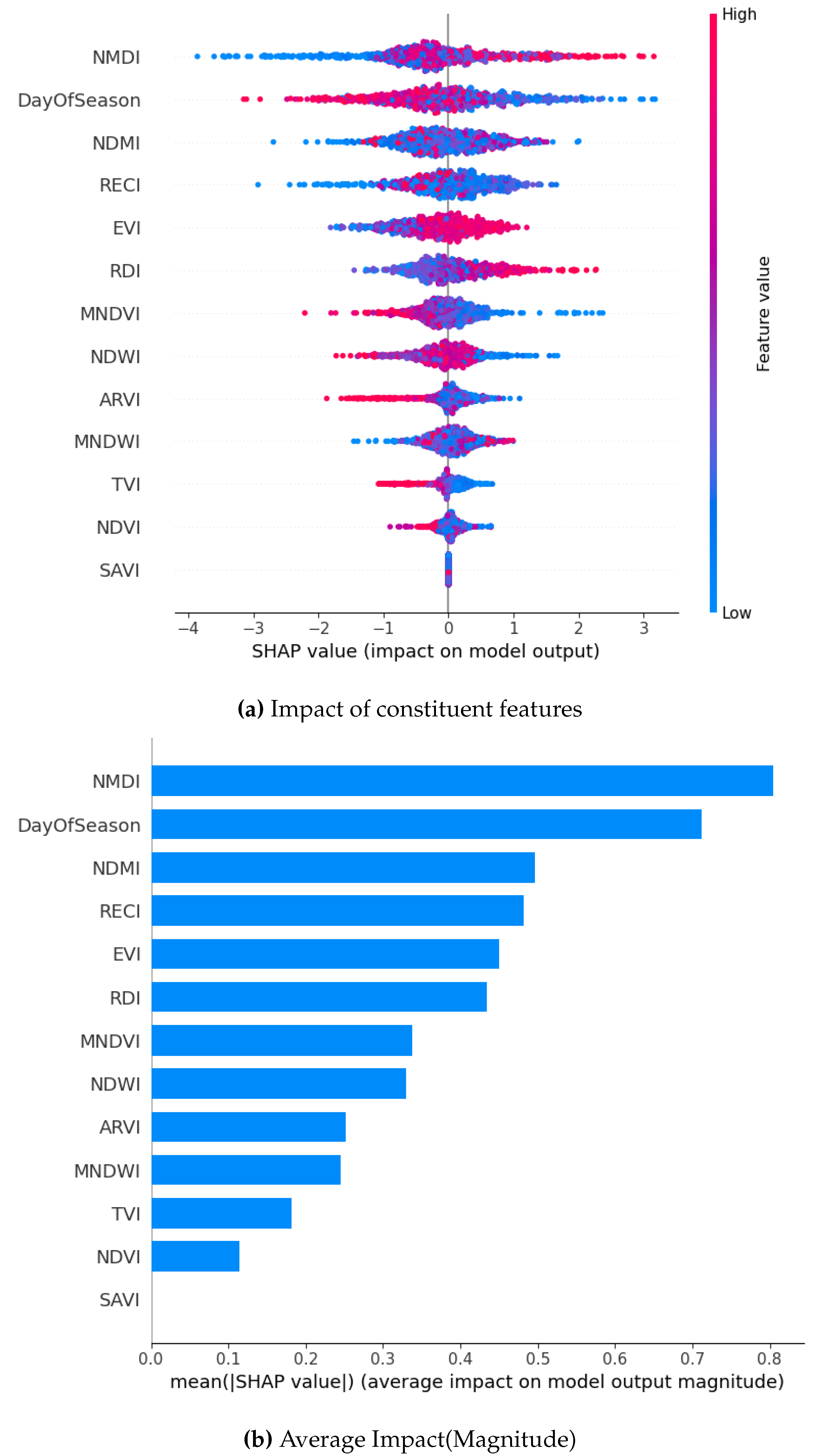
Figure 6.
SHAP Visualization Summary For Random Forest before oversampling.
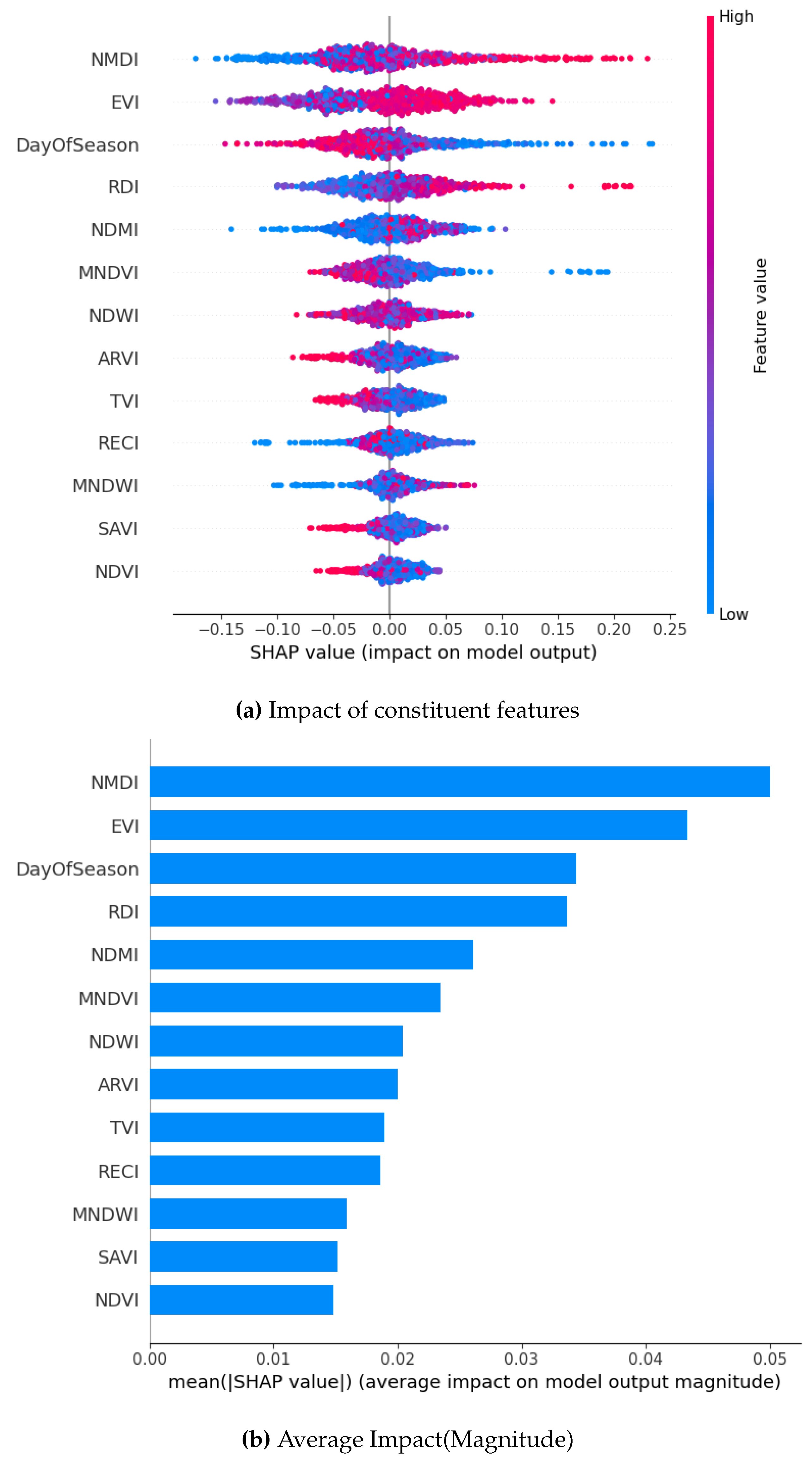
Figure 7.
SHAP Visualization Summary For Bagging Technique before oversampling.
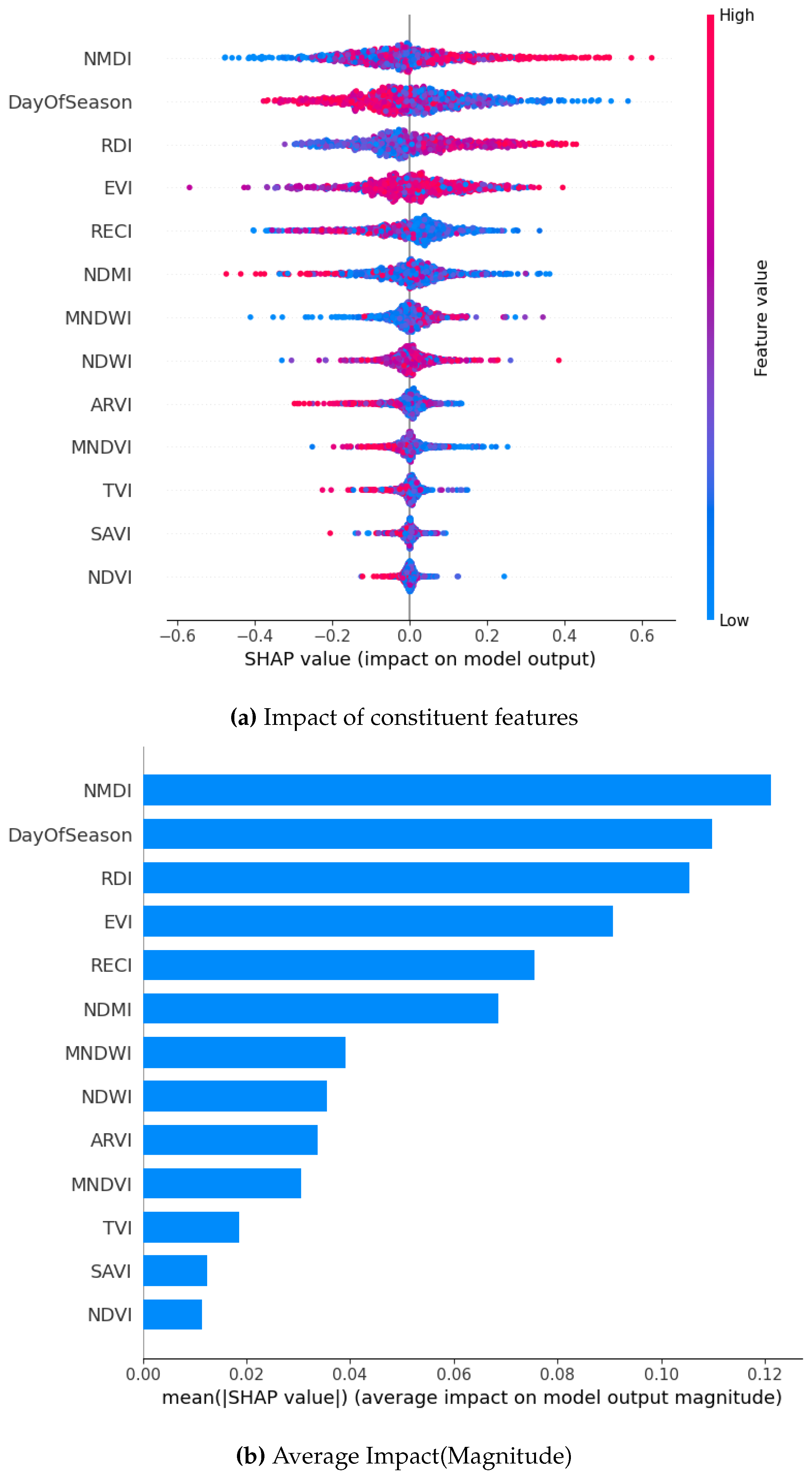
Figure 8.
SHAP Visualization Summary For Gradient Boost before oversampling.
7.4.2. SMOTE
From the magnitude of the SHAP values resulting from our analysis, we observe that DOS emerges as the most significant feature followed closely by NMDI. It is the top contributor for both the XGBoost and Gradient Boosting models. RECI and EVI also demonstrate consistent importance in all models. Notably, RDI is the top contributor for the Bagging classifier and remains consistently among the top 4-5 features in other models. SAVI, NDVI, and TVI consistently show narrow spreads around zero, indicating minimal impact across predictions for all the models. Their influence is low in magnitude and consistent across data points, making them the least important features. SHAP values are mostly concentrated around zero in the Gradient Boosting model, particularly for the DOS feature. This suggests that DOS may have both positive and negative impacts on predictions across different samples, resulting in an overall distribution centered around zero. Similarly, NMDI and EVI also have a highly concentrated distribution. NMDI is slightly negative on average, while EVI contributes more to the positive results. Both NMDI and EVI exhibit a highly concentrated distribution of SHAP values. NMDI demonstrates a slightly negative mean SHAP value, providing a marginal contribution towards the classification of non-drought conditions. In contrast, EVI displays a more positive mean SHAP value, which contributes significantly to the classification of drought conditions. With Bagging Classifier, RDI exhibits the widest spread in SHAP values among the top features, which suggests that variations in this feature can lead to both strong positive and negative contributions to the prediction. EVI shows a somewhat narrower dispersion compared to RDI. This indicates that while it is important, its effect on the model is less variable. EVI’s distribution is slightly skewed with many points concentrated on the positive side.
Figure 9.
SHAP Visualization Summary For XG Boost using SMOTE.
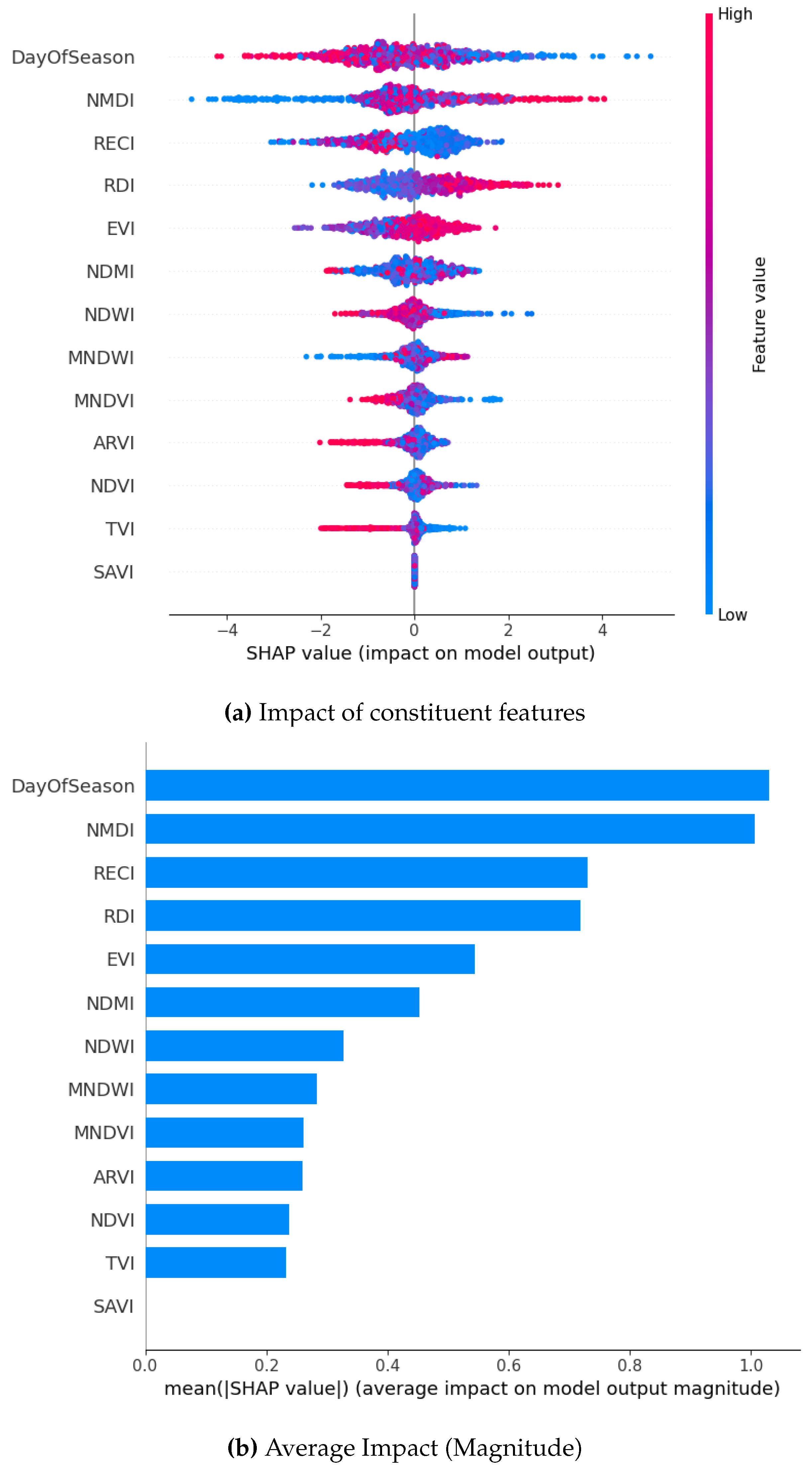
Figure 10.
SHAP Visualization Summary For Random Forest using SMOTE.
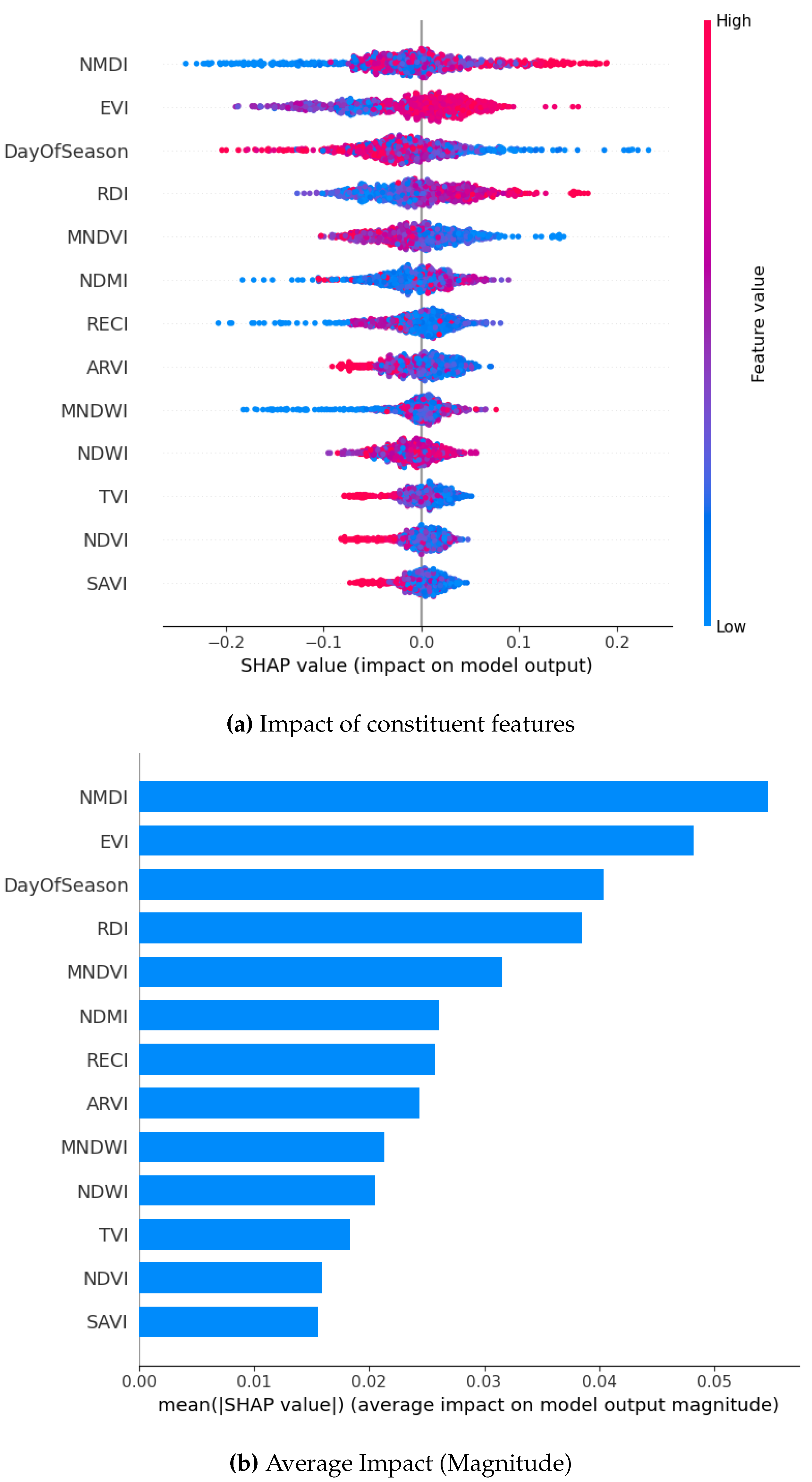
Figure 11.
SHAP Visualization Summary For Bagging Technique using SMOTE.
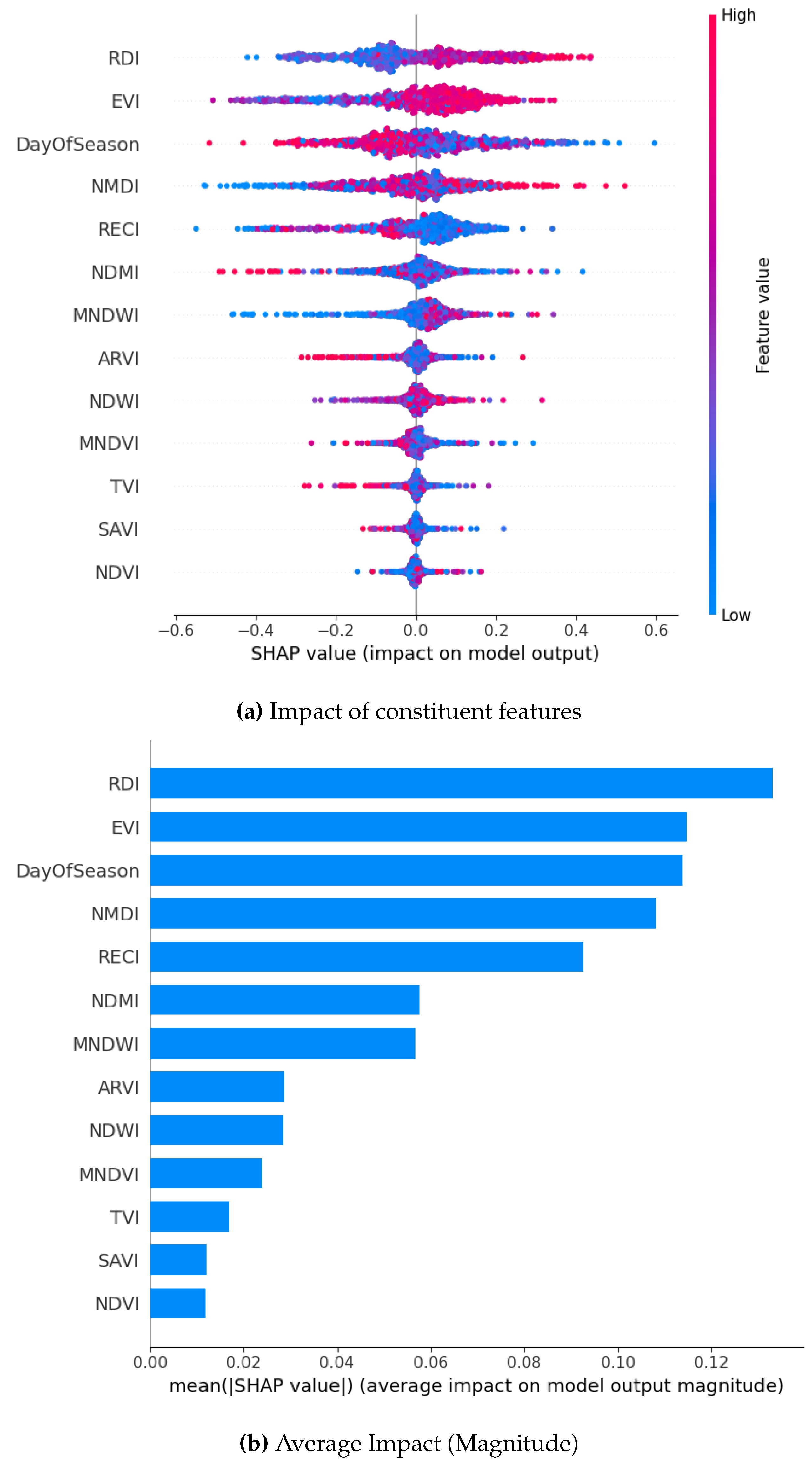
Figure 12.
SHAP Visualization Summary For Gradient Boost using SMOTE.
7.4.3. SMOTE Borderline
For the borderline SMOTE, DOS and NMDI emerge as top contributors for two models each when focusing on the magnitude of the SHAP analysis. This is followed by EVI, RDI, and RECI. On the contrary, SAVI, NDVI, and TVI consistently rank as the least-contributing features across the models.
Figure 13.
SHAP Visualization Summary For XG Boost using SMOTE Borderline

Figure 14.
SHAP Visualization Summary For Random Forest using SMOTE Borderline.
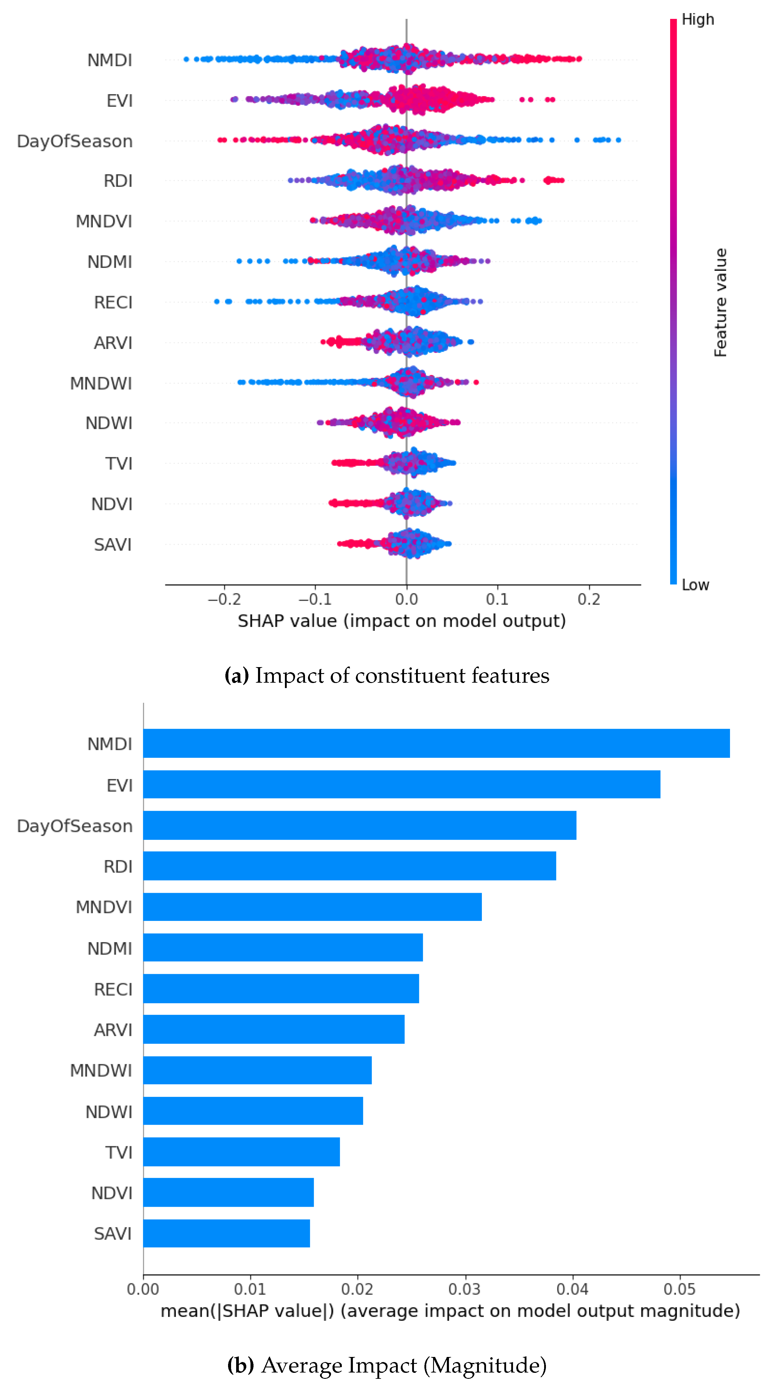
Figure 15.
SHAP Visualization Summary For Bagging Technique using SMOTE Borderline.

Figure 16.
SHAP Visualization Summary For Gradient Boost using SMOTE Borderline.
7.4.4. AdaSyn
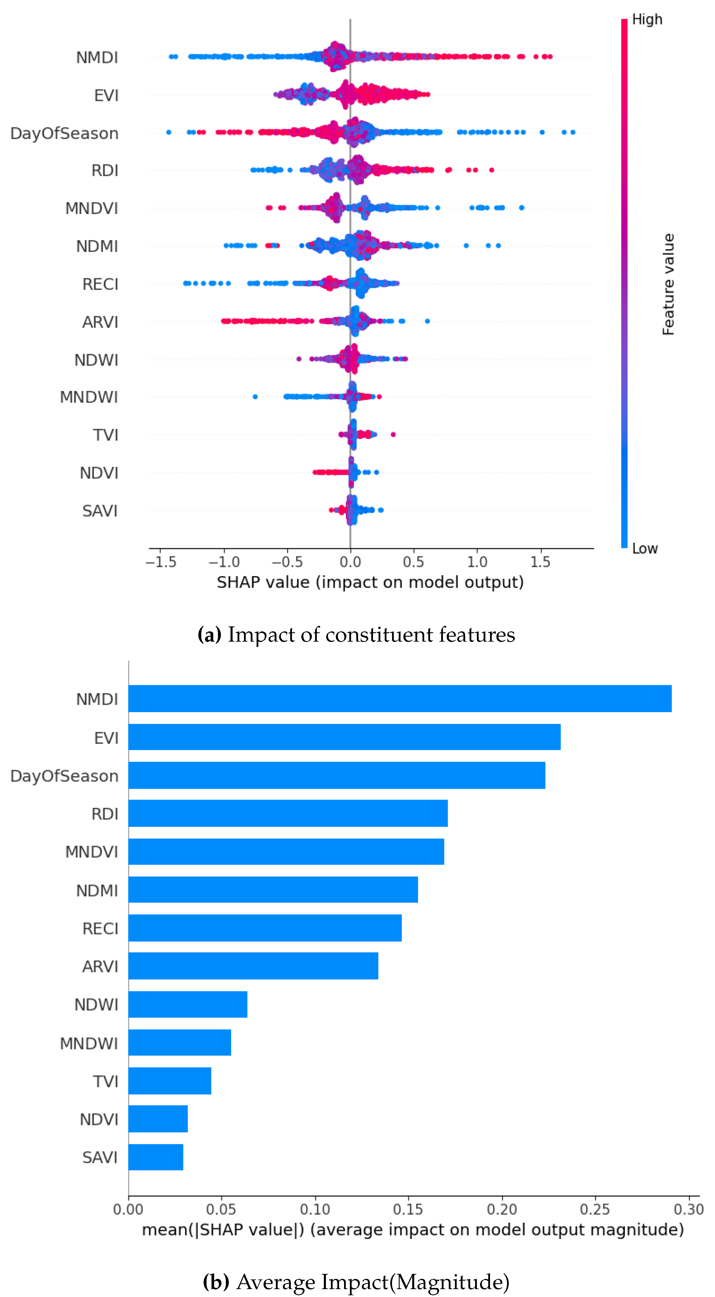
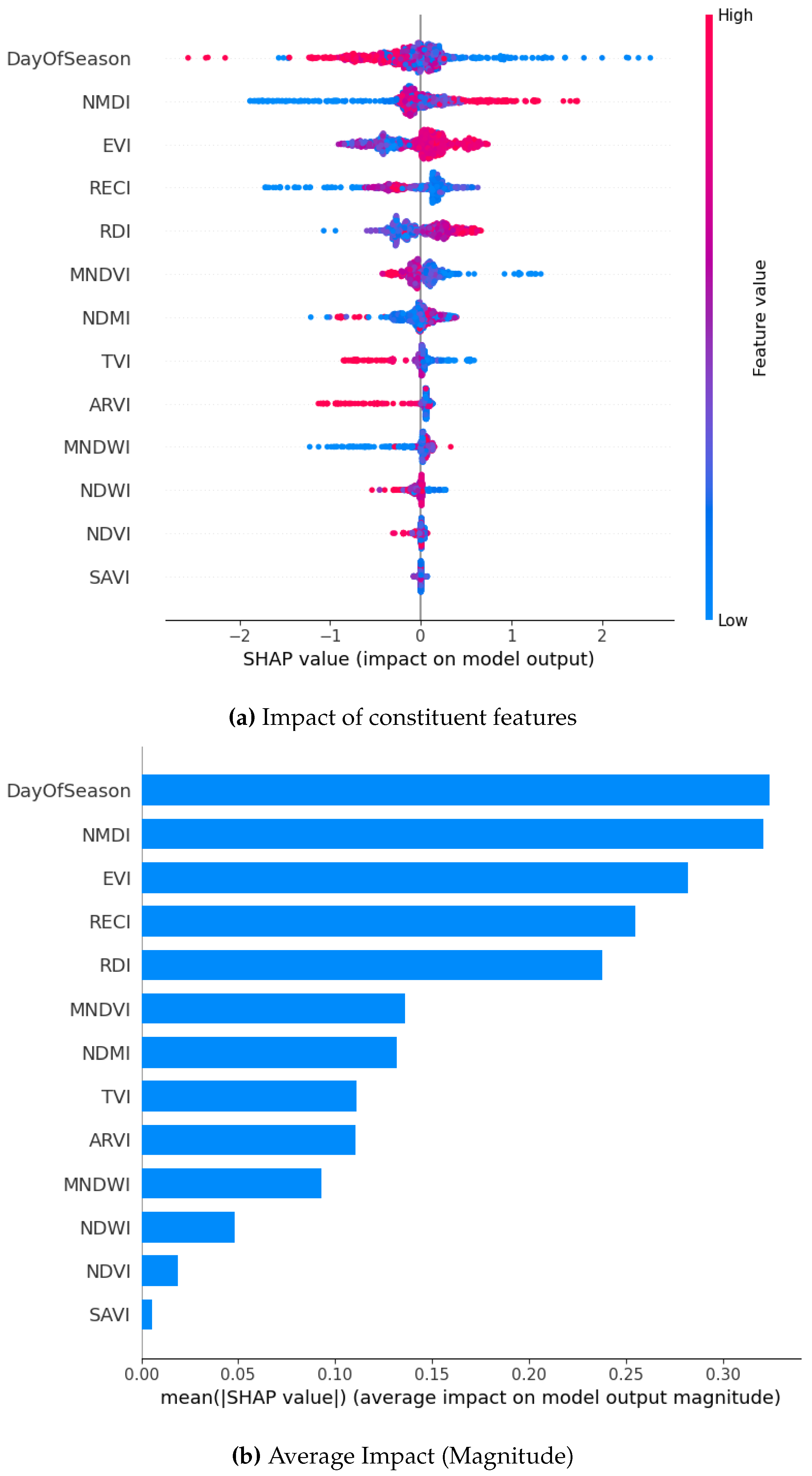
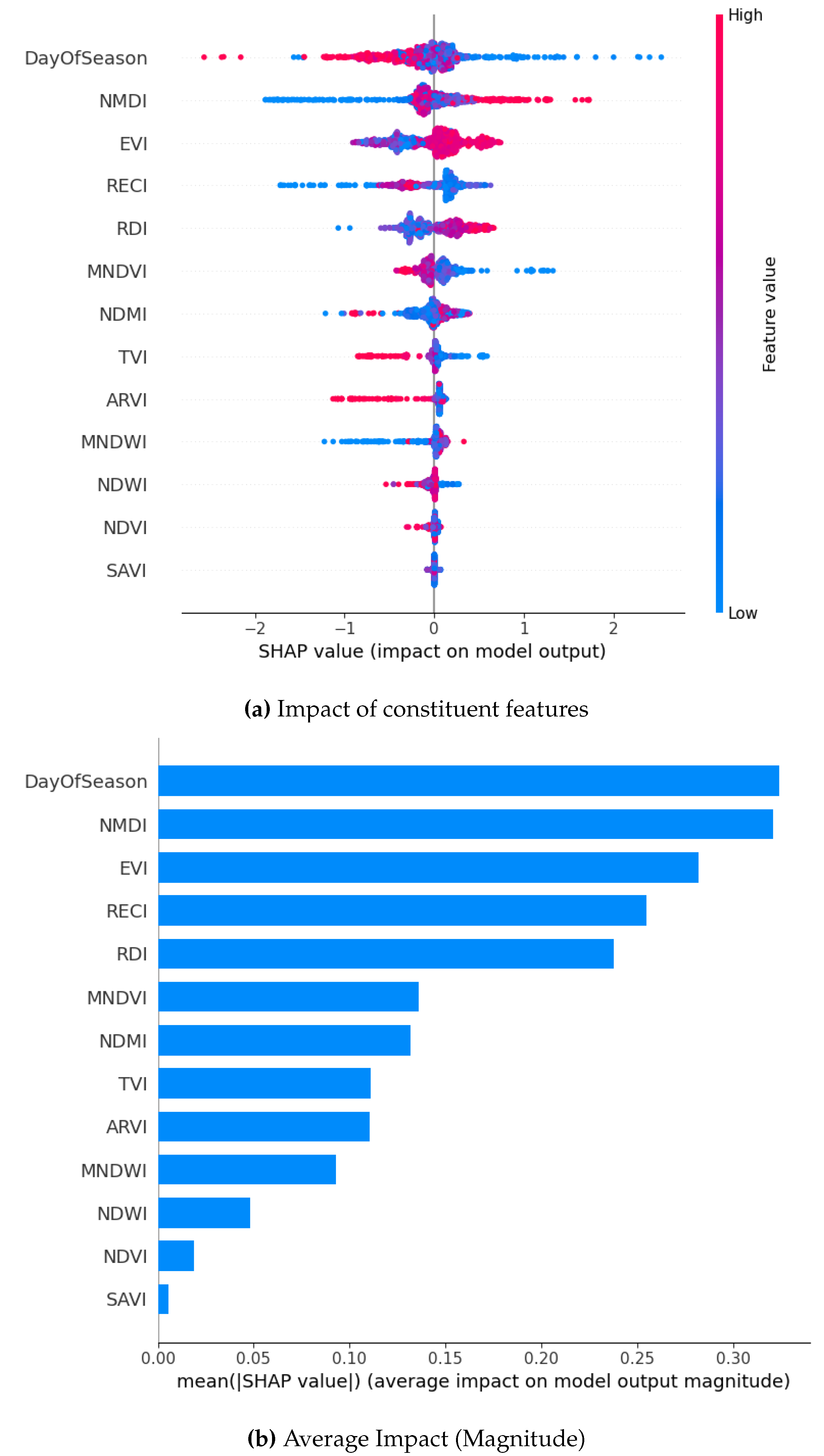
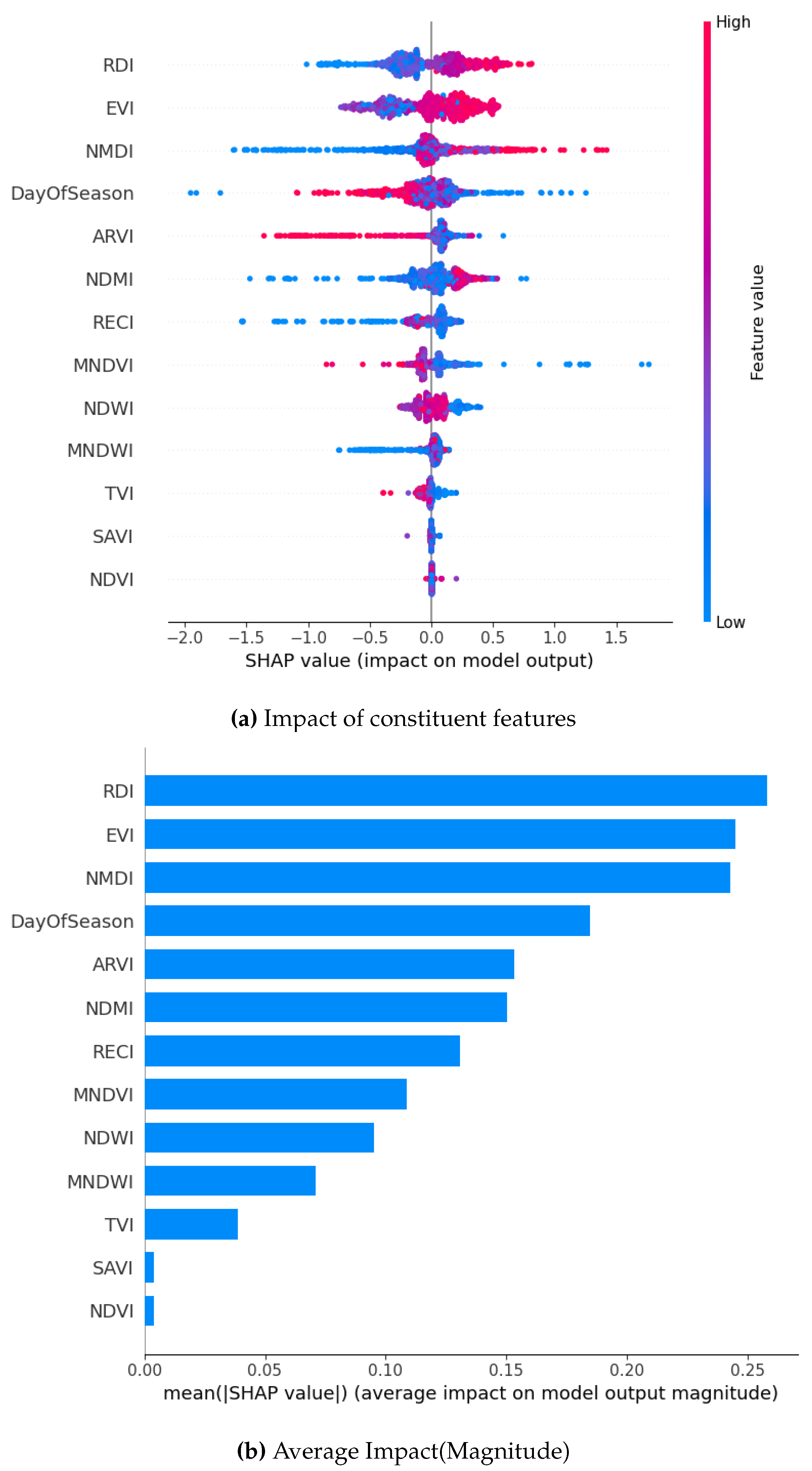
While using the ADASYN method to oversample across all models, RDI, NMDI, and DOS unfailingly emerge as the most influential features. They have high SHAP values indicating a huge impact on the model output. For example, in the XGBoost model, NMDI and DayOfSeason exhibit the highest SHAP values, ranging up to 3, suggesting a notable positive influence on predictions. Similarly, in the GB model, RDI and EVI show high SHAP values, with a broader range (-2.0 to 1.5), indicating both positive and negative impacts depending on feature values. The Bagging and RF models have similar tendencies but they also have a narrower range of SHAP values (Bagging: -0.4 to 0.6; RF: -0.2 to 0.2), suggesting a more moderate influence of features.
Whereas, SAVI and NDVI consistently have the lowest SHAP values across all models. This implies minimal impact on predictions. The SHAP summary plots also stress the variability in feature importance across models, with XGBoost showing the most pronounced feature impacts, followed by GB, Bagging, and RF. This detailed analysis highlights the critical role of RDI, NMDI, and DOS in driving model predictions, while also revealing model-specific differences in feature sensitivity and impact magnitude.
Figure 17.
SHAP Visualization Summary For XG Boost using ADASYN.
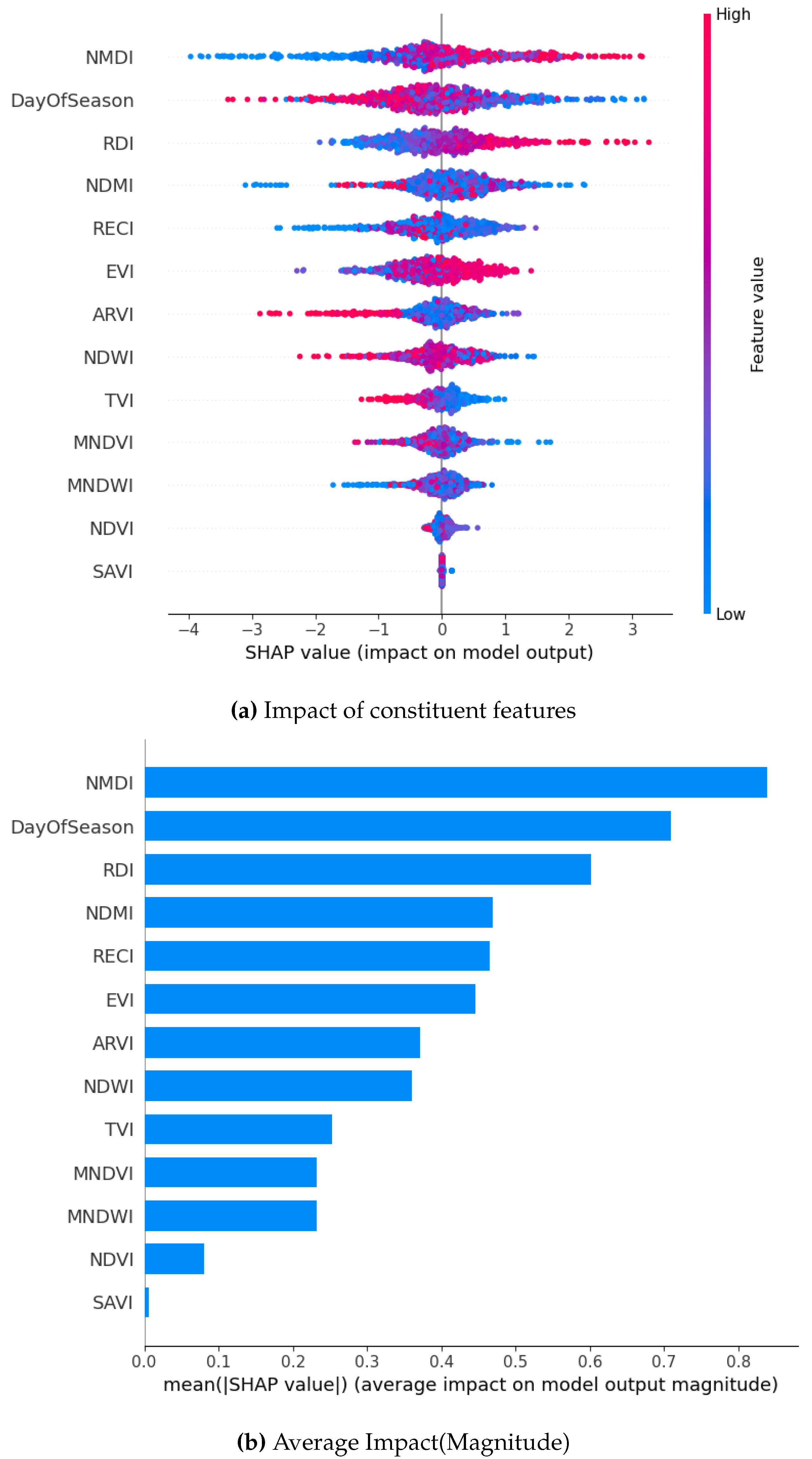
Figure 18.
SHAP Visualization Summary For Random Forest using ADASYN.
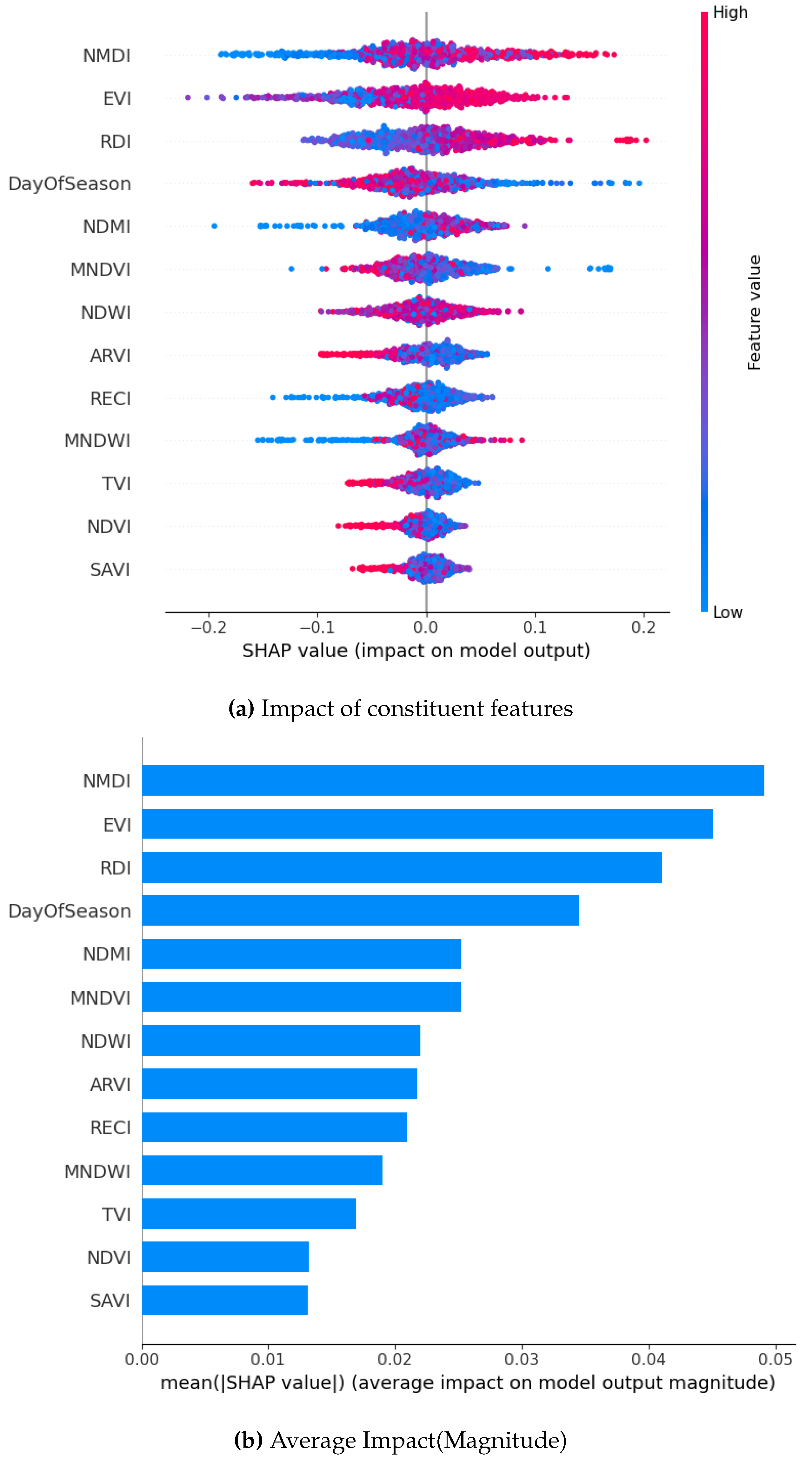
Figure 19.
SHAP Visualization Summary For Bagging Technique using ADASYN.
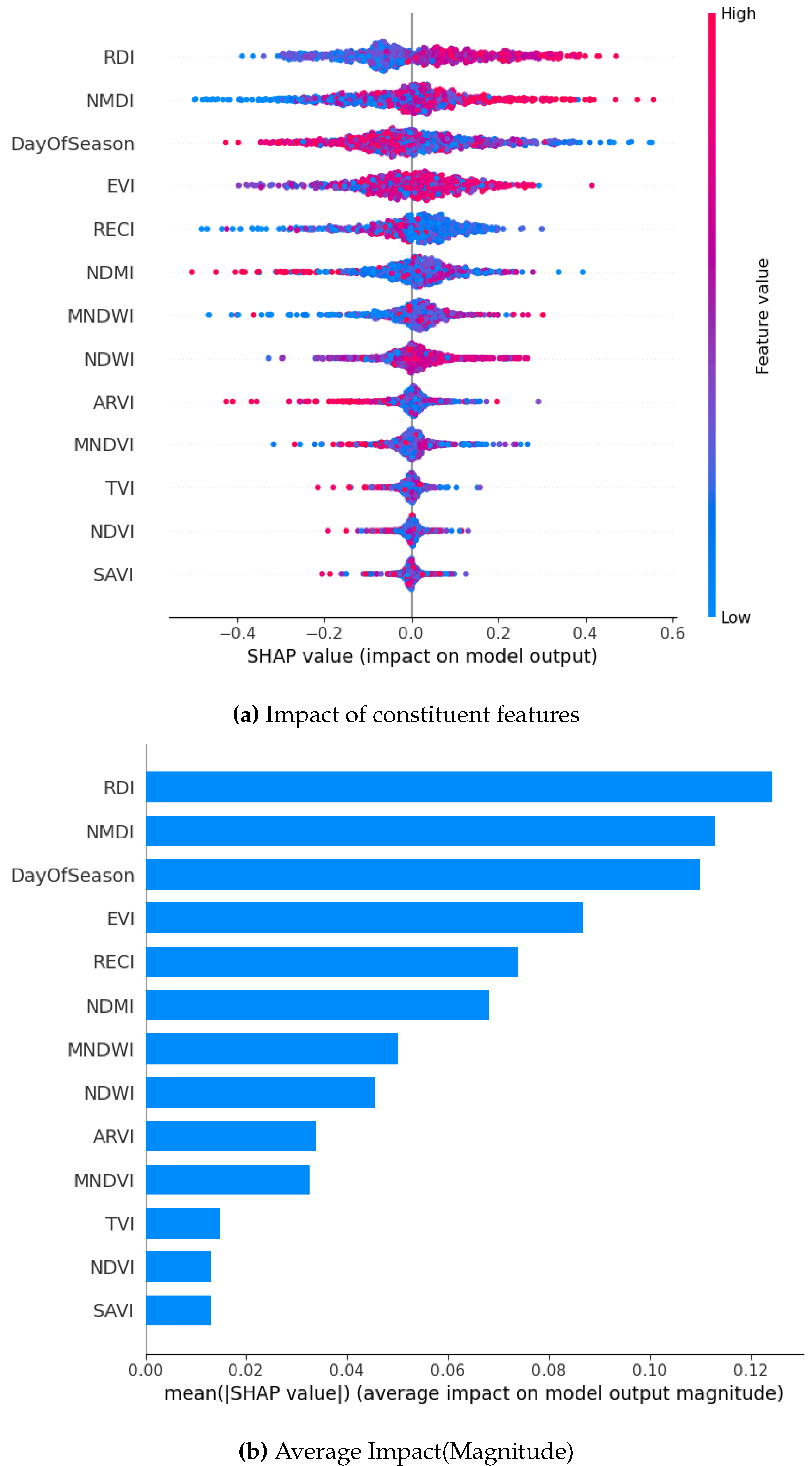
Figure 20.
SHAP Visualization Summary For Gradient Boost using ADASYN.
7.5. Model Aggregation for Most Relevant Features
One of the objectives of this work is to find the most influential spectral indices for the separation of drought and non-drought. Spectral indices vary in their sensitivity to drought-related changes in vegetation, soil moisture, and canopy structure. Different features influence machine algorithms differently based on their internal mechanisms. Further, each machine learning algorithm has its own distinctive advantages. As an example, XGB is well-suited for non-linear relationships, whereas RF and BGN use ensemble averaging and random subspace sampling to reduce variance, making them more robust to noise. Hence, relying on a single algorithm risks overlooking critical features that are algorithm-specific or context-dependent. Thus, a consensus is required to aggregate feature importance rankings across algorithms such that it could identify the features consistently influential across diverse model assumptions. Borda count and weighted sum are used here in model aggregation. Borda count is simple to interpret and works with ranks, not with associated scores. Hence, it is less sensitive to extreme values and treats all models equally, avoiding bias toward any single algorithm. It is better suited when all the models are equally trusted, as it is observed that XGB, RF, and BGN perform similarly in some cases. However, Borda count ignores the magnitude of importance, such as a feature ranked 1st in one model and 10th in another is treated the same as a feature ranked 5th in both. Weighted sum incorporates magnitudes of importance along with the aggregation. Though the weighted sum may be found sensitive to outliers, its performance improves when unbiased contributions can be summarized such as in SHAP. Hence, both Borda count and weighted sum are used as discussed below.
7.5.1. Before Oversampling
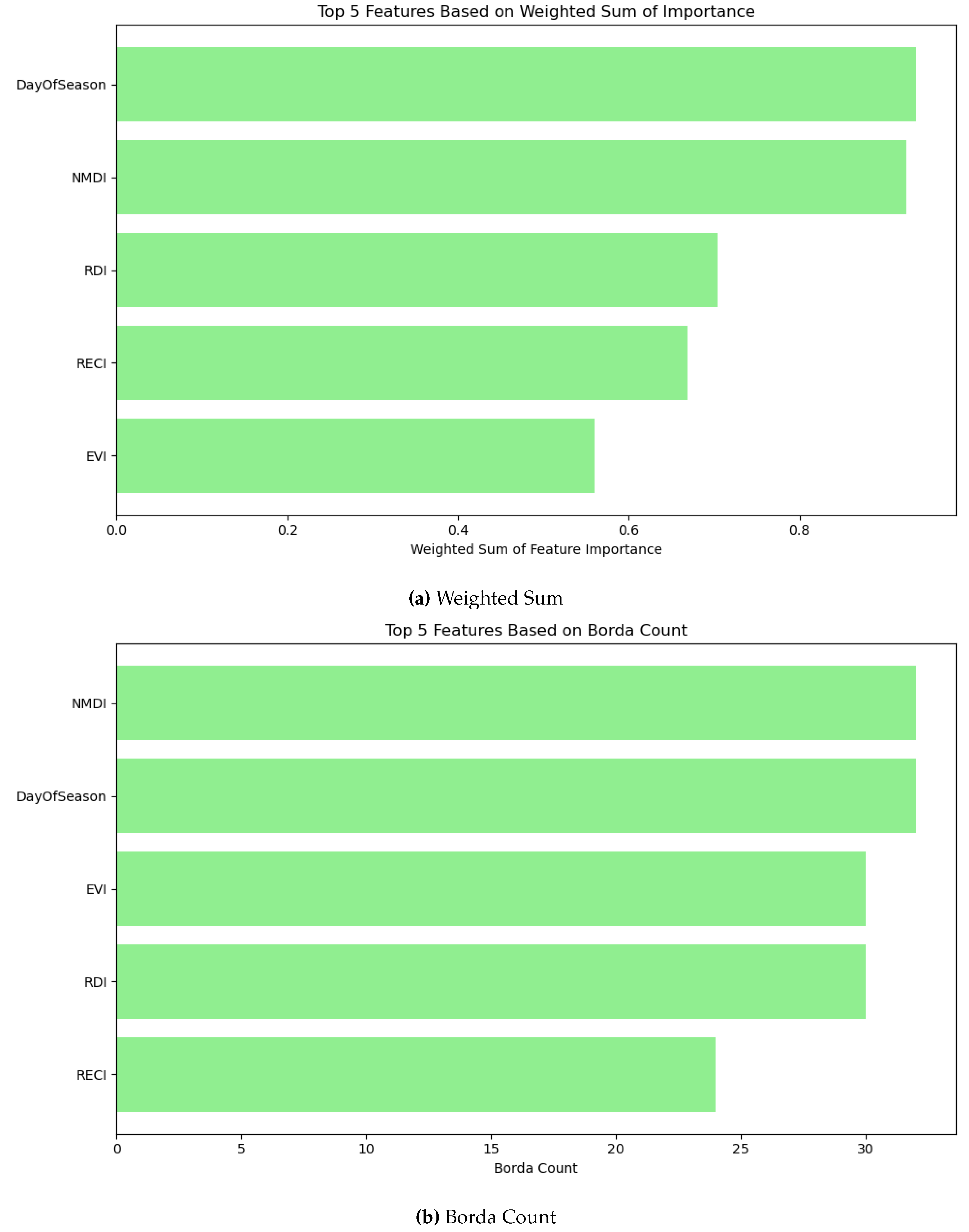
The top five features based on weighted sum and Borda count are shown in Figure 21a and Figure 21b, respectively. It can be shown that though the top two features are NMDI and DOS in both the aggregators, the top five features are different by Borda count and weighted sum. In weighted sum, NDMI is the third most influential feature whereas, it is fifth in Borda count. RDI can be found in the top five feature only in Borda count, however RECI is found in the top five features of weighted sum. The aggregators agree with four features to in the top five, i.e. NMDI, DOS, NDMI, and EVI. To further understand their influence, the top features are employed by the machine learning techniques to asses their performance as shown in Table 15 (weighted sum), and Table 16 (Borda count). It can be observed that the top feature (NMDI) contribute significantly in both cases. The combination of NMDI, and DOS provides accuracy in XGB, RF, BGN in all cases. Hence, NMDI and DOS contribute significantly to the classification. Expanding the feature set to include the top 3–4 features yielded marginal improvements. The top 5 features in Borda count achieve an accuracy level close to that of using all features. However, the top 5 features in the weighted sum provide less accuracy. Borda count and weighted sum have four common feaures, whereas Borda count includes RDI and weighted sum includes RECI. Hence, RDI can be considered as more influential than RECI.
7.5.2. SMOTE
Aggregations were also studied through SMOTE. It can be observed that the top five features in weighted sum and Borda count are similar, however their rankings are different. NMDI, and DOS are the top most influential features in both cases with different rankings. However, their scores are marginally different. NMDI, and DOS were also top two influential features before oversampling. EVI was also found influential before oversampling and in SMOTE. Notably, NDMI, which was influential before oversampling, is absent in both these cases. The performance by top features in weighted sum and Borda count are shown in Table 17 and Table 18, respectively. The top two features significantly contribute to the performance in both cases. The inclusion of EVI improves the performance. Notably, though the top five features are same, their performance differs in weighted sum and Bodra count based on their ranking.
Figure 22.
Model Aggregation for 5 most relevant features in SMOTE.
7.5.3. Borderline SMOTE
As shown in Figure 23 same five features, DOS, NMDI, RECI, EVI, and RDI are found most important features with different rankings in borderline SMOTE. NDMI is absent as top features. DOS, and NMDI are found top two influential features with high ranking. As shown in Table 19 (weighted sum), and Table 20 (Borda Count), these two features capture the essential signal for accurate predictions, providing accuracy. Alongside, it can be observed that the inclusion of RDI also boosts the performance.
7.5.4. ADASYN
The top features are similar in ADASYN with SMOTE, and borderline SMOTE. The ranking of the features are different in weighted sum and Borda count. Hence, NDMI, which is absent after all the oversampling techniques, may provide significance to the majority class. NMDI, RDI, and DOS provide significant performance in both weighted sum and Borda count. Feature subsets selected via weighted ranking yield accuracy comparable to using all features, demonstrating that dimensionality reduction can be achieved without sacrificing predictive power. However, the Borda count method yields comparatively lower accuracy. Thus, rankings derived from the weighted sum approach should also be prioritized.
Figure 24.
Model Aggregation for 5 most relevant features in ADASYN.
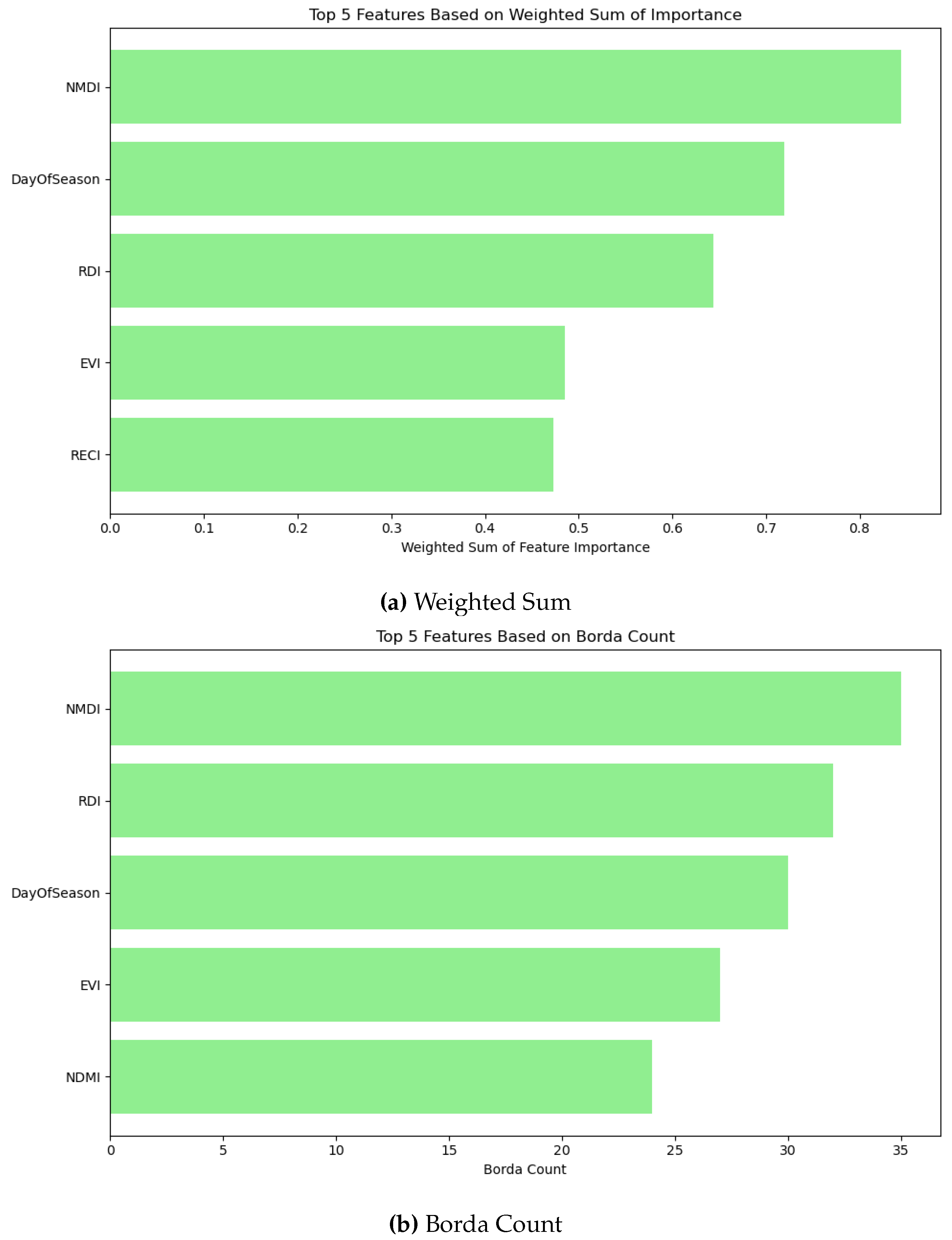
Table 21.
Model performance of Top 1 to Top 5 feature using Weighted Sum in ADASYN.
| XGBoost | Random Forest | Bagging | Gradient Boosting | |
|---|---|---|---|---|
| Top 1 | Acc: 0.5657 Prec: 0.4596 Rec: 0.5632 |
Acc: 0.5917 Prec: 0.4866 Rec: 0.5989 |
Acc: 0.5917 Prec: 0.4866 Rec: 0.5989 |
Acc: 0.5907 Prec: 0.4867 Rec: 0.6511 |
| Top 2 | Acc: 0.6938 Prec: 0.5958 Rec: 0.7005 |
Acc: 0.7112 Prec: 0.6184 Rec: 0.7033 |
Acc: 0.6721 Prec: 0.5735 Rec: 0.6648 |
Acc: 0.6308 Prec: 0.5267 Rec: 0.6511 |
| Top 3 | Acc: 0.7687 Prec: 0.6752 Rec: 0.7995 |
Acc: 0.7904 Prec: 0.7050 Rec: 0.8077 |
Acc: 0.7828 Prec: 0.6962 Rec: 0.7995 |
Acc: 0.6504 Prec: 0.5467 Rec: 0.6758 |
| Top 4 | Acc: 0.7709 Prec: 0.6852 Rec: 0.7775 |
Acc: 0.7926 Prec: 0.7235 Rec: 0.7692 |
Acc: 0.7839 Prec: 0.7165 Rec: 0.7500 |
Acc: 0.6786 Prec: 0.5766 Rec: 0.7033 |
| Top 5 | Acc: 0.8230 Prec: 0.7445 Rec: 0.8407 |
Acc: 0.8165 Prec: 0.7456 Rec: 0.8132 |
Acc: 0.8187 Prec: 0.7599 Rec: 0.7912 |
Acc: 0.6960 Prec: 0.5929 Rec: 0.7363 |
Table 22.
Model performance of Top 1 to Top 5 feature using Borda Count in ADASYN.
| XGBoost | Random Forest | Bagging | Gradient Boosting | |
|---|---|---|---|---|
| Top 1 | Acc: 0.5657 Prec: 0.4596 Rec: 0.5632 |
Acc: 0.5917 Prec: 0.4866 Rec: 0.5989 |
Acc: 0.5917 Prec: 0.4866 Rec: 0.5989 |
Acc: 0.5907 Prec: 0.4867 Rec: 0.6511 |
| Top 2 | Acc: 0.6298 Prec: 0.5277 Rec: 0.6016 |
Acc: 0.6406 Prec: 0.5394 Rec: 0.6209 |
Acc: 0.6547 Prec: 0.5553 Rec: 0.6346 |
Acc: 0.6135 Prec: 0.5092 Rec: 0.6099 |
| Top 3 | Acc: 0.7687 Prec: 0.6752 Rec: 0.7995 |
Acc: 0.7980 Prec: 0.7150 Rec: 0.8132 |
Acc: 0.7828 Prec: 0.6962 Rec: 0.7995 |
Acc: 0.6504 Prec: 0.5467 Rec: 0.6758 |
| Top 4 | Acc: 0.7883 Prec: 0.7161 Rec: 0.7692 |
Acc: 0.7937 Prec: 0.7219 Rec: 0.7775 |
Acc: 0.7861 Prec: 0.7169 Rec: 0.7582 |
Acc: 0.6786 Prec: 0.5766 Rec: 0.7033 |
| Top 5 | Acc: 0.8132 Prec: 0.7319 Rec: 0.8324 |
Acc: 0.8165 Prec: 0.7519 Rec: 0.7995 |
Acc: 0.8056 Prec: 0.7354 Rec: 0.7940 |
Acc: 0.7036 Prec: 0.6056 Rec: 0.7170 |
Notably, in all cases, the top feature provides accuracy just slightly better than chance or random guessing (). However, accuracy significantly improves with the addition of the second and third best features. This suggests that no single feature alone is sufficient to reliably predict drought, hence detection of drought requires combining multiple factors. The most influential feature alone does not separate classes well, but it still plays a key role when combined with others. The second and third most influential features may complement or refine the information provided by the most influential feature, as supported by the accuracy boost. However, second and third most influential features alone may not perform well without the first. The significant leap in accuracy suggests a synergistic effect where these features work better together. Further insights and experimentation are regarded as future works.
8. Conclusion
Droughts can have severe consequences, particularly in the agricultural sector where reduced water availability may catastrophically impact crop yields and food quality. As an agrarian nation characterized by climatic diversity, India faces severe repercussions from agricultural droughts, making their early detection particularly useful albeit challenging. Spectral indices and machine learning techniques are exhaustively used in multi-spectral images to detect droughts. However, the influence of different spectral and temporal parameters on detecting drought in different climatic locations of India has not been thoroughly investigated yet. This study explores the use of multispectral Sentinel-2 remote sensing indices and machine learning techniques to detect drought conditions in three distinct regions of India such as Jodhpur, Amravati, and Thanjavur during the Rabi season (October to April).
One of the key contributions of this work lies in the a structured ground-truth drought dataset for Rabi seasons across six years and three diverse regions. This ground truth was compiled by analyzing formal drought declarations from government sources and corroborating them regional and national news publications across the country. Different machine learning algorithms were employed, fed with twelve spectral indices and one temporal index. To enable the application of machine learning models, we incorporated district-year level ground truth table to assign drought labels. From this district-year level table, a binary drought label (“Drought” = 1, “No Drought” = 0) was derived. Importantly, this seasonal label was assigned to every individual observation in the time-series dataset as an additional column. Since each observation corresponds to a specific day within a Rabi season, this approach effectively links seasonal drought status to daily-level satellite measurements. This enabled training of machine learning models on a high-resolution time-series dataset while preserving the integrity of seasonal drought definitions in the labeling process. When trained and evaluated on the individual satellite index records each representing a single date within the Rabi season for a given district, all models were assessed based on their ability to classify each such record as either drought or no drought. In this setting, Bagging Classifier has highest accuracy(84.15%) followed closely by Random Forest((83.39%) and XGBoost(82.30%) with Gradient Boosting(74.59%) at last position. To align model output with the seasonal nature of drought declarations, we introduced a seasonal aggregation strategy: for each district and Rabi season, we applied a majority vote over the predicted labels of all its observations. This approach led to over accuracy, precision and recall for XGBoost, Random Forest, and Bagging Classifier in identifying drought and non-drought seasons.
In addition to the accuracy assessment, we conducted a detailed feature importance analysis using SHAP values, which assign an interpretable impact score to each feature. To consolidate rankings across models, we used a consensus-based Borda count method and a magnitude-based weighted sum of SHAP values. According to the Borda count ranking, the five most influential features were NMDI, DOS, NDMI, RECI, and EVI. In contrast, the weighted sum of SHAP values identified NMDI, DOS, NDMI, EVI, and RDI as the top contributors. Oversampling methods - SMOTE, Borderline SMOTE, and ADASYN were used to mitigate class imbalance caused by fewer drought-labeled observations. Exhaustive error analysis and studies on data imbalance over these algorithms provide more insights on the data distribution. It is observed from this case study that the Normalized Multi-band Drought Index (NMDI) and Day-of-the-Season (DOS) are found to be the two most important features across all the models and oversampling techniques. It has also been observed that they contribute significantly to achieving an accuracy figure closer to the level obtained using the complete feature set. Our experimentation shows that the data distribution of drought and non-drought using these spectral and temporal indices has complex and non-linear decision boundary, which makes machine learning a more promising approach for their classification than classical approaches based on smooth likelihood functions. Findings from our work provides useful clues on how to assess drought conditions in the Rabi season across diverse regions of India leveraging multispectral optical spaceborne data. Further it provides insights on the influence of different features and data distributions, which could support future investigation of the problem. Focusing on interpretable variables, the findings may be relevant to stakeholders in climate science and agriculture, empowering them to design targeted mitigation strategies and improve resilience planning.
Funding
This research was partially supported by the “Nord Ovest Digitale e Sostenibile (NODES)” project, which has been granted funding through the MUR – M4C2 1.5 of PNRR, under the European Union’s NextGenerationEU initiative (Grant agreement No. ECS00000036).
References
- Urban, M.; Berger, C.; Mudau, T.E.; Heckel, K.; Truckenbrodt, J.; Onyango Odipo, V.; Smit, I.P.; Schmullius, C. Surface moisture and vegetation cover analysis for drought monitoring in the southern Kruger National Park using Sentinel-1, Sentinel-2, and Landsat-8. Remote Sensing 2018, 10, 1482. [Google Scholar] [CrossRef]
- Gimeno-Sotelo, L.; Sorí, R.; Nieto, R.; Vicente-Serrano, S.M.; Gimeno, L. Unravelling the origin of the atmospheric moisture deficit that leads to droughts. Nature Water 2024, 2, 242–253. [Google Scholar] [CrossRef]
- AghaKouchak, A.; Farahmand, A.; Melton, F.S.; Teixeira, J.; Anderson, M.C.; Wardlow, B.D.; Hain, C.R. Remote sensing of drought: Progress, challenges and opportunities. Reviews of Geophysics 2015, 53, 452–480. [Google Scholar] [CrossRef]
- Zhang, Y.; Hao, Z.; Feng, S.; Zhang, X.; Xu, Y.; Hao, F. Agricultural drought prediction in China based on drought propagation and large-scale drivers. Agricultural Water Management 2021, 255, 107028. [Google Scholar] [CrossRef]
- Satapathy, T.; Dietrich, J.; Ramadas, M. Agricultural drought monitoring and early warning at the regional scale using a remote sensing-based combined index. Environmental Monitoring and Assessment 2024, 196, 1132. [Google Scholar] [CrossRef]
- Sorooshian, S.; AghaKouchak, A.; Arkin, P.; Eylander, J.; Foufoula-Georgiou, E.; Harmon, R.; Hendrickx, J.M.; Imam, B.; Kuligowski, R.; Skahill, B.; et al. Advanced concepts on remote sensing of precipitation at multiple scales. Bulletin of the American Meteorological Society 2011, 92, 1353–1357. [Google Scholar] [CrossRef]
- Anderson, M.C.; Hain, C.; Wardlow, B.; Pimstein, A.; Mecikalski, J.R.; Kustas, W.P. Evaluation of drought indices based on thermal remote sensing of evapotranspiration over the continental United States. Journal of Climate 2011, 24, 2025–2044. [Google Scholar] [CrossRef]
- Heim Jr, R.R. A review of twentieth-century drought indices used in the United States. Bulletin of the American Meteorological Society 2002, 83, 1149–1166. [Google Scholar] [CrossRef]
- Xie, F.; Fan, H. Deriving drought indices from MODIS vegetation indices (NDVI/EVI) and Land Surface Temperature (LST): Is data reconstruction necessary? International Journal of applied earth observation and geoinformation 2021, 101, 102352. [Google Scholar] [CrossRef]
- Gu, Y.; Brown, J.F.; Verdin, J.P.; Wardlow, B. A five-year analysis of MODIS NDVI and NDWI for grassland drought assessment over the central Great Plains of the United States. Geophysical research letters 2007, 34. [Google Scholar] [CrossRef]
- Nam, W.H.; Tadesse, T.; Wardlow, B.D.; Hayes, M.J.; Svoboda, M.D.; Hong, E.M.; Pachepsky, Y.A.; Jang, M.W. Developing the vegetation drought response index for South Korea (VegDRI-SKorea) to assess the vegetation condition during drought events. International journal of remote sensing 2018, 39, 1548–1574. [Google Scholar] [CrossRef]
- Parkash, V.; Singh, S. A review on potential plant-based water stress indicators for vegetable crops. Sustainability 2020, 12, 3945. [Google Scholar] [CrossRef]
- Martínez-Fernández, J.; González-Zamora, A.; Sánchez, N.; Gumuzzio, A.; Herrero-Jiménez, C. Satellite soil moisture for agricultural drought monitoring: Assessment of the SMOS derived Soil Water Deficit Index. Remote Sensing of Environment 2016, 177, 277–286. [Google Scholar] [CrossRef]
- Anderson, M.C.; Zolin, C.A.; Sentelhas, P.C.; Hain, C.R.; Semmens, K.; Yilmaz, M.T.; Gao, F.; Otkin, J.A.; Tetrault, R. The Evaporative Stress Index as an indicator of agricultural drought in Brazil: An assessment based on crop yield impacts. Remote Sensing of Environment 2016, 174, 82–99. [Google Scholar] [CrossRef]
- Mu, Q.; Zhao, M.; Kimball, J.S.; McDowell, N.G.; Running, S.W. A remotely sensed global terrestrial drought severity index. Bulletin of the American Meteorological Society 2013, 94, 83–98. [Google Scholar] [CrossRef]
- Dilip, T.; Kumari, M.; Murthy, C.; Neelima, T.; Chakraborty, A.; Devi, M.U. Monitoring early-season agricultural drought using temporal Sentinel-1 SAR-based combined drought index. Environmental Monitoring and Assessment 2023, 195, 925. [Google Scholar] [CrossRef]
- Volden, E. New Capabilities in Earth Observation for Agriculture, 2017.
- Varghese, D.; Radulović, M.; Stojković, S.; Crnojević, V. Reviewing the potential of Sentinel-2 in assessing the drought. Remote sensing 2021, 13, 3355. [Google Scholar] [CrossRef]
- Wang, Q.; Blackburn, G.A.; Onojeghuo, A.O.; Dash, J.; Zhou, L.; Zhang, Y.; Atkinson, P.M. Fusion of Landsat 8 OLI and Sentinel-2 MSI data. IEEE Transactions on Geoscience and Remote Sensing 2017, 55, 3885–3899. [Google Scholar] [CrossRef]
- Thanh Noi, P.; Kappas, M. Comparison of random forest, k-nearest neighbor, and support vector machine classifiers for land cover classification using Sentinel-2 imagery. Sensors 2017, 18, 18. [Google Scholar] [CrossRef]
- Ferrant, S.; Selles, A.; Le Page, M.; Mermoz, S.; Gascoin, S.; Bouvet, A.; Ahmed, S.; Kerr, Y.H.; et al. Sentinel-1&2 for near real time cropping pattern monitoring in drought prone areas. application to irrigation water needs in telangana, south-india. International Archives of the Photogrammetry, Remote Sensing and Spatial Information Sciences 2019, 42, 285–292. [Google Scholar]
- Zhang, L.; Liu, Y.; Ren, L.; Teuling, A.J.; Zhu, Y.; Wei, L.; Zhang, L.; Jiang, S.; Yang, X.; Fang, X.; et al. Analysis of flash droughts in China using machine learning. Hydrology and Earth System Sciences 2022, 26, 3241–3261. [Google Scholar] [CrossRef]
- Gupta, A.; Kaur, L.; Kaur, G. Drought stress detection technique for wheat crop using machine learning. PeerJ Computer Science 2023, 9, e1268. [Google Scholar] [CrossRef]
- Mokhtar, A.; Jalali, M.; He, H.; Al-Ansari, N.; Elbeltagi, A.; Alsafadi, K.; Abdo, H.G.; Sammen, S.S.; Gyasi-Agyei, Y.; Rodrigo-Comino, J. Estimation of SPEI meteorological drought using machine learning algorithms. IEEe Access 2021, 9, 65503–65523. [Google Scholar] [CrossRef]
- Sriram, K.; Suresh, K. Machine learning perspective for predicting agricultural droughts using Naïve Bayes algorithm. Middle-East J Sci Res 2016, 24, 178–184. [Google Scholar]
- Lee, C.S.; Sohn, E.; Park, J.D.; Jang, J.D. Estimation of soil moisture using deep learning based on satellite data: A case study of South Korea. GIScience & Remote Sensing 2019, 56, 43–67. [Google Scholar]
- Feng, P.; Wang, B.; Li Liu, D.; Yu, Q. Machine learning-based integration of remotely-sensed drought factors can improve the estimation of agricultural drought in South-Eastern Australia. Agricultural Systems 2019, 173, 303–316. [Google Scholar] [CrossRef]
- Prodhan, F.A.; Zhang, J.; Hasan, S.S.; Sharma, T.P.P.; Mohana, H.P. A review of machine learning methods for drought hazard monitoring and forecasting: Current research trends, challenges, and future research directions. Environmental modelling & software 2022, 149, 105327. [Google Scholar]
- Bowen, D.; Ungar, L. Generalized SHAP: Generating multiple types of explanations in machine learning. arXiv 2020, arXiv:2006.07155. [Google Scholar]
- Saari, D.G. Selecting a voting method: the case for the Borda count. Constitutional Political Economy 2023, 34, 357–366. [Google Scholar] [CrossRef]
- West, H.; Quinn, N.; Horswell, M.; White, P. Assessing vegetation response to soil moisture fluctuation under extreme drought using sentinel-2. Water 2018, 10, 838. [Google Scholar] [CrossRef]
- Huete, A.; Justice, C.; Van Leeuwen, W. MODIS vegetation index (MOD13). Algorithm theoretical basis document 1999, 3, 295–309. [Google Scholar]
- Jopia, A.; Zambrano, F.; Pérez-Martínez, W.; Vidal-Páez, P.; Molina, J.; De la Hoz Mardones, F. Time-series of vegetation indices (VNIR/SWIR) derived from Sentinel-2 (A/B) to assess turgor pressure in kiwifruit. ISPRS International Journal of Geo-Information 2020, 9, 641. [Google Scholar] [CrossRef]
- Jiang, Z.; Huete, A.R.; Didan, K.; Miura, T. Development of a two-band enhanced vegetation index without a blue band. Remote sensing of Environment 2008, 112, 3833–3845. [Google Scholar] [CrossRef]
- Sentinel Hub. Atmospherically Resistant Vegetation Index (ARVI). Available online: https://custom-scripts.sentinel-hub.com/sentinel-2/arvi/ (accessed on 27 January 2024).
- Marshall, G.; Zhou, X. Drought detection in semi-arid regions using remote sensing of vegetation indices and drought indices. In Proceedings of the IGARSS 2004. 2004 IEEE International Geoscience and Remote Sensing Symposium. IEEE; 2004; Vol. 3, pp. 1555–1558. [Google Scholar]
- Kaufman, Y.J.; Tanre, D. Atmospherically resistant vegetation index (ARVI) for EOS-MODIS. IEEE transactions on Geoscience and Remote Sensing 1992, 30, 261–270. [Google Scholar] [CrossRef]
- Ahmed, T.; Javed, N.; Faisal, M.; Sadia, H. A framework for smart agriculture system to monitor the crop stress and drought stress using sentinel-2 satellite image. In Proceedings of 3rd International Conference on Artificial Intelligence: Advances and Applications: ICAIAA 2022; Springer, 2023; pp. 345–361. [Google Scholar]
- McFeeters, S.K. The use of the Normalized Difference Water Index (NDWI) in the delineation of open water features. International journal of remote sensing 1996, 17, 1425–1432. [Google Scholar] [CrossRef]
- Huete, A.R. A soil-adjusted vegetation index (SAVI). Remote sensing of environment 1988, 25, 295–309. [Google Scholar] [CrossRef]
- Sun, C.; Li, J.; Cao, L.; Liu, Y.; Jin, S.; Zhao, B. Evaluation of vegetation index-based curve fitting models for accurate classification of salt marsh vegetation using sentinel-2 time-series. Sensors 2020, 20, 5551. [Google Scholar] [CrossRef]
- Nellis, M.D.; Briggs, J.M. Transformed vegetation index for measuring spatial variation in drought impacted biomass on Konza Prairie, Kansas. Transactions of the Kansas Academy of Science (1903) 1992, 93–99. [Google Scholar] [CrossRef]
- Gu, Z.; Zeng, Z.; Shi, X.; Yu, D.; Zheng, W.; Zhang, Z.; Hu, Z. Estimating models of vegetation fractional coverage based on remote sensing images at different radiometric correction levels. Frontiers of Forestry in China 2009, 4, 402–408. [Google Scholar] [CrossRef]
- Strashok, O.; Ziemiańska, M.; Strashok, V. Evaluation and Correlation of Sentinel-2 NDVI and NDMI in Kyiv (2017–2021). Journal of Ecological Engineering 2022, 23. [Google Scholar] [CrossRef]
- Sentinel Hub. Normalized Difference Moisture Index (NDMI). https://custom-scripts.sentinel-hub.com/sentinel-2/ndmi/, 2024. [Accessed: 27-Jan-2024].
- Wang, L.; Qu, J.J. NMDI: A normalized multi-band drought index for monitoring soil and vegetation moisture with satellite remote sensing. Geophysical Research Letters 2007, 34. [Google Scholar] [CrossRef]
- Zhang, H.w.; Chen, H.l. The Application of Modified Normalized Difference Water Index (MNDWI) by Leaf Area Index in the Retrieval of Regional Drought Monitoring. The International Archives of the Photogrammetry, Remote Sensing and Spatial Information Sciences 2015, 40, 141–147. [Google Scholar] [CrossRef]
- Xu, H. Modification of normalised difference water index (NDWI) to enhance open water features in remotely sensed imagery. International journal of remote sensing 2006, 27, 3025–3033. [Google Scholar] [CrossRef]
- Jurgens, C. The modified normalized difference vegetation index (mNDVI) a new index to determine frost damages in agriculture based on Landsat TM data. International Journal of Remote Sensing 1997, 18, 3583–3594. [Google Scholar] [CrossRef]
- Dong, Z.; Wang, L.; Gao, M.; Zhu, X.; Feng, W.; Li, N. Ratio Drought Index (RDI): A soil moisture index based on new NIR-red triangle space. International Journal of Remote Sensing 2024, 45, 6976–6989. [Google Scholar] [CrossRef]
- EOS Data Analytics. Chlorophyll Index: Overview, Calculation, and Application. https://eos.com/make-an-analysis/chlorophyll-index/, 2024. [Accessed: 27-Jan-2024].
- Sentinel Hub. Red-edge Chlorophyll Index (RECI). https://custom-scripts.sentinel-hub.com/custom-scripts/sentinel-2/chl_rededge/, 2024. [Accessed: 27-Jan-2024].
- Jafarzadeh, H.; Mahdianpari, M.; Gill, E.; Mohammadimanesh, F.; Homayouni, S. Bagging and boosting ensemble classifiers for classification of multispectral, hyperspectral and PolSAR data: a comparative evaluation. Remote Sensing 2021, 13, 4405. [Google Scholar] [CrossRef]
- Shao, Z.; Ahmad, M.N.; Javed, A. Comparison of Random Forest and XGBoost Classifiers Using Integrated Optical and SAR Features for Mapping Urban Impervious Surface. Remote Sensing 2024, 16, 665. [Google Scholar] [CrossRef]
- Breiman, L. Random forests. Machine learning 2001, 45, 5–32. [Google Scholar] [CrossRef]
- Friedman, J.H. Greedy function approximation: a gradient boosting machine. Annals of statistics 2001, pp. 1189–1232.
- Chen, T.; Guestrin, C. Xgboost: A scalable tree boosting system. In Proceedings of the Proceedings of the 22nd acm sigkdd international conference on knowledge discovery and data mining, 2016, pp.
- Breiman, L. Bagging predictors. Machine learning 1996, 24, 123–140. [Google Scholar] [CrossRef]
- Shapley, L.S. A value for n-person games. Contribution to the Theory of Games 1953, 2. [Google Scholar]
- Lundberg, S.M.; Lee, S.I. A unified approach to interpreting model predictions. In Proceedings of the Proceedings of the 31st International Conference on Neural Information Processing Systems, 2017, NIPS’17, p.
- Lundberg, S.M.; Erion, G.; Chen, H.; DeGrave, A.; Prutkin, J.M.; Nair, B.; Katz, R.; Himmelfarb, J.; Bansal, N.; Lee, S.I. From local explanations to global understanding with explainable AI for trees. Nature Machine Intelligence 2020, 2, 56–67. [Google Scholar] [CrossRef] [PubMed]
- Pacuit, E. Voting methods 2011.
- Churchman, C.W.; Ackoff, R.L. An approximate measure of value. Journal of the Operations Research Society of America 1954, 2, 172–187. [Google Scholar] [CrossRef]
- Chawla, N.V.; Bowyer, K.W.; Hall, L.O.; Kegelmeyer, W.P. SMOTE: synthetic minority over-sampling technique. Journal of artificial intelligence research 2002, 16, 321–357. [Google Scholar] [CrossRef]
- Han, H.; Wang, W.Y.; Mao, B.H. Borderline-SMOTE: a new over-sampling method in imbalanced data sets learning. In Proceedings of the International conference on intelligent computing. Springer; 2005; pp. 878–887. [Google Scholar]
- He, H.; Bai, Y.; Garcia, E.A.; Li, S. ADASYN: Adaptive synthetic sampling approach for imbalanced learning. In Proceedings of the 2008 IEEE international joint conference on neural networks (IEEE world congress on computational intelligence). Ieee; 2008; pp. 1322–1328. [Google Scholar]
- Food and Agriculture Organization of the United Nations. FAO Global Administrative Unit Layers (GAUL) 2015. http://www.fao.org/geospatial/gb/en/products/gaul/index.html. [Accessed: 27-Jan-2024].
- Copernicus. Copernicus Global Land Cover. https://land.copernicus.eu/global/lc. [Accessed: 27-Jan-2024].
- (ISRO), I.S.R.O. Drought Assessment Using Remote Sensing and GIS: Drought Manual 2020. Technical report, National Remote Sensing Centre (NRSC), ISRO, 2020.
- (ISRO), I.S.R.O. Agri-DSS Help Manual. Technical report, National Remote Sensing Centre (NRSC), ISRO, 2020.
- Mishra, V.; Singh, M.; Ghosh, S.; et al. Monitoring Agricultural Drought in India Using Multisource Remote Sensing Indicators. Environmental Challenges 2021, 4, 100021. [Google Scholar]
- The Hindu. 19 Districts in Rajasthan Drought Hit. https://www.thehindu.com/news/national/other-states/19-districts-in-rajasthan-droughthit/article8491809.ece, 2016. Accessed: 2025-02-07.
- Factly. 266 Districts in 11 Different States Declared Drought-Affected (2015-16). https://factly.in/266-districts-11-different-states-drought-affected-2015-16/, 2016. Accessed: 2025-02-07.
- Parliament of India. Drought Fund Allocation Status (2017). https://sansad.in/getFile/loksabhaquestions/annex/14/AU4057.pdf?source=pqals, 2017. Accessed: 2025-02-07.
- Firstpost Editor. Drought in Rajasthan: Over Rs 7000 Crore Spent on Projects But Not Much Water Has Flown Through Western Region. https://www.firstpost.com/india/drought-in-rajasthan-over-rs-7000-crore-spent-on-projects-but-not-much-water-has-flown-through-western-region-6331911.html, 2019. Accessed: 2025-02-07.
- ANI. Rajasthan Govt Declares 5555 Villages as Drought-Affected. https://www.aninews.in/news/national/general-news/rajasthan-govt-declares-5555-villages-as-drought-affected20190306224744/, 2019. Accessed: 2025-02-07.
- The Statesman. 1388 Villages in Rajasthan Declared Drought-Affected by State Govt. https://www.thestatesman.com/india/1388-villages-in-rajasthan-declared-drought-affected-by-state-govt-1502820817.html, 2019. Accessed: 2025-02-07.
- NDTV. More Than 1,000 Villages in 4 Districts of Rajasthan Affected by Drought. https://www.ndtv.com/india-news/more-than-1-000-villages-in-4-districts-of-rajasthan-affected-by-draught-2130998, 2019. Accessed: 2025-02-07.
- Government of India. Annexure to Lok Sabha Question AU454: Central Assistance for Drought. https://sansad.in/getFile/loksabhaquestions/annex/177/AU454.pdf?source=pqals, 2020. Accessed: 2025-02-07.
- Economic Times. Maharashtra Government Declares Drought in 29,000 Villages. https://economictimes.indiatimes.com/news/politics-and-nation/maharashtra-government-declares-drought-in-29000-villages/articleshow/52238372.cms?from=mdr, 2016. Accessed: 2025-02-07.
- Hindustan Times. Maharashtra declares drought; 26 districts hit. https: //www.hindustantimes.com/mumbai-news/maharashtra-declares-drought-26-districts-hit/story-ETaPfo9owb7yVW8EQ1lQGL.html, 2018. [Google Scholar]
- Times of India. Eight of 11 Vidarbha districts declared drought-hit. https://timesofindia.indiatimes.com/city/nagpur/8-of-11-vid-dists-declared-drought-hitryots-say-need-more-sops-to-tackle-crisis/articleshow/66595394.cms, 2018. Accessed: 2025-02-07.
- Times of India. Drought brings down Rabi crop area by 40% in 2018-19. https://timesofindia.indiatimes.com/city/pune/drought-brings-down-rabi-crop-area-by-40-in-2018-19/articleshow/67949533.cms, 2019. Accessed: 2025-02-07.
- Hindu, T. Rain causes immense damage to huts and paddy fields. https://www.thehindu.com/news/national/tamil-nadu/rain-causes-immense-damage-to-huts-and-paddy-fields/article7882286.ece, 2015. Accessed: 2025-02-07.
- Reports, S. Drought-Affected States Report AU981. https://sansad.in/getFile/loksabhaquestions/annex/15/AU981.pdf?source=pqals, 2016. Accessed: 2025-02-07.
- Moneylife. Retreating Monsoon Worst in 140 Years, TN Declares Drought as 144 Farmers Die. https://www.moneylife.in/article/retreating-monsoon-worst-in-140-years-tn-declares-drought-as-144-farmers-die/49433.html, 2017. Accessed: 2025-02-07.
- Tamil Nadu Agricultural Department. Government Order on Drought Declaration. https://www.tnagrisnet.tn.gov.in/fcms/documents/go/20-GO.No.29-2(2).pdf, 2017. Accessed: 2025-02-07.
- Hindu, T. Heavy rain in Tiruvarur and Thanjavur districts. https://www.thehindu.com/news/cities/Tiruchirapalli/heavy-rain-in-tiruvarur-and-thanjavur-districts/article19991157.ece, 2017. Accessed: 2025-02-07.
- New Indian Express. 24 districts declared as drought-hit; number to rise in coming months. https://www.newindianexpress.com/states/tamil-nadu/2019/Mar/21/24-districts-declared-as-drought-hit-number-to-rise-in-coming-months-1953962.html, 2019. Accessed: 2025-02-07.
- Bricks, N. Tamil Nadu Weather Forecast December 12, 2019. https://www.newsbricks.com/tamil-nadu/tamil-nadu-weather-forecast-december-12-2019/67258, 2019. Accessed: 2025-02-07.
- Weather.com. Northeast Monsoon to Commence Over South India From , 2020. https://weather.com/en-IN/india/news/news/2020-10-27-northeast-monsoon-commence-over-south-india-from-october-28, 2020. Accessed: 2025-02-07. 28 October.
- of India, T. Disasters That Struck India in 2020. https://timesofindia.indiatimes.com/india/disasters-that-struck-india-in-2020/articleshow/79954339.cms, 2020. Accessed: 2025-02-07.
- Mongabay. Though Cyclone Nivar Had a Soft Landing, Floods Hit Coastal Districts. https://india.mongabay.com/2020/12/though-cyclone-nivar-had-a-soft-landing-floods-hit-coastal-districts/, 2020. Accessed: 2025-02-07.
Figure 1.
Location of the Ground Truth Districts
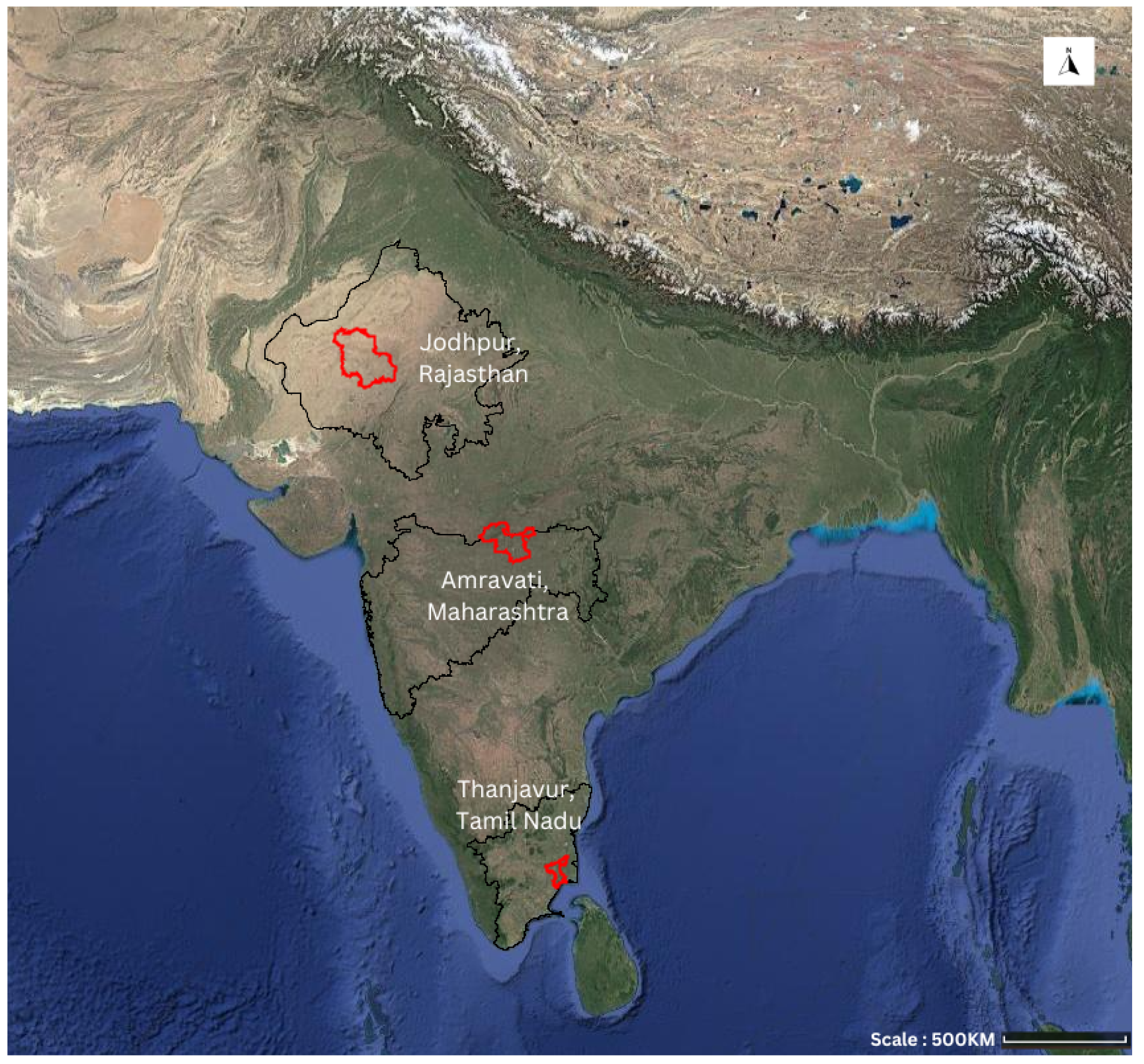
Figure 2.
Drought Declaration Workflow In India
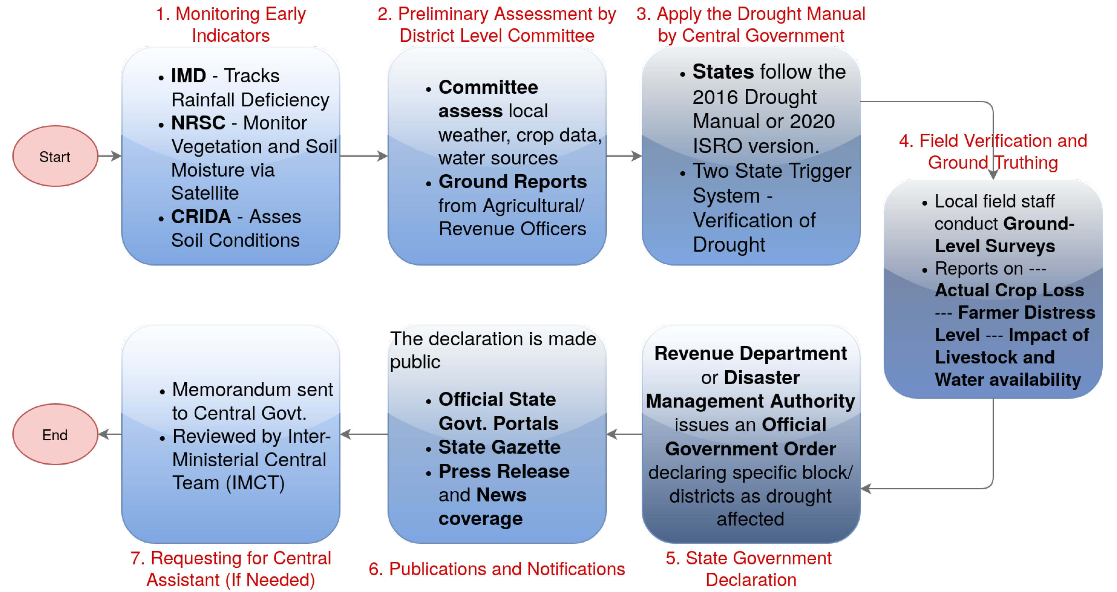
Figure 3.
Data Acquisition and Preprocessing Workflow with Google Earth Engine
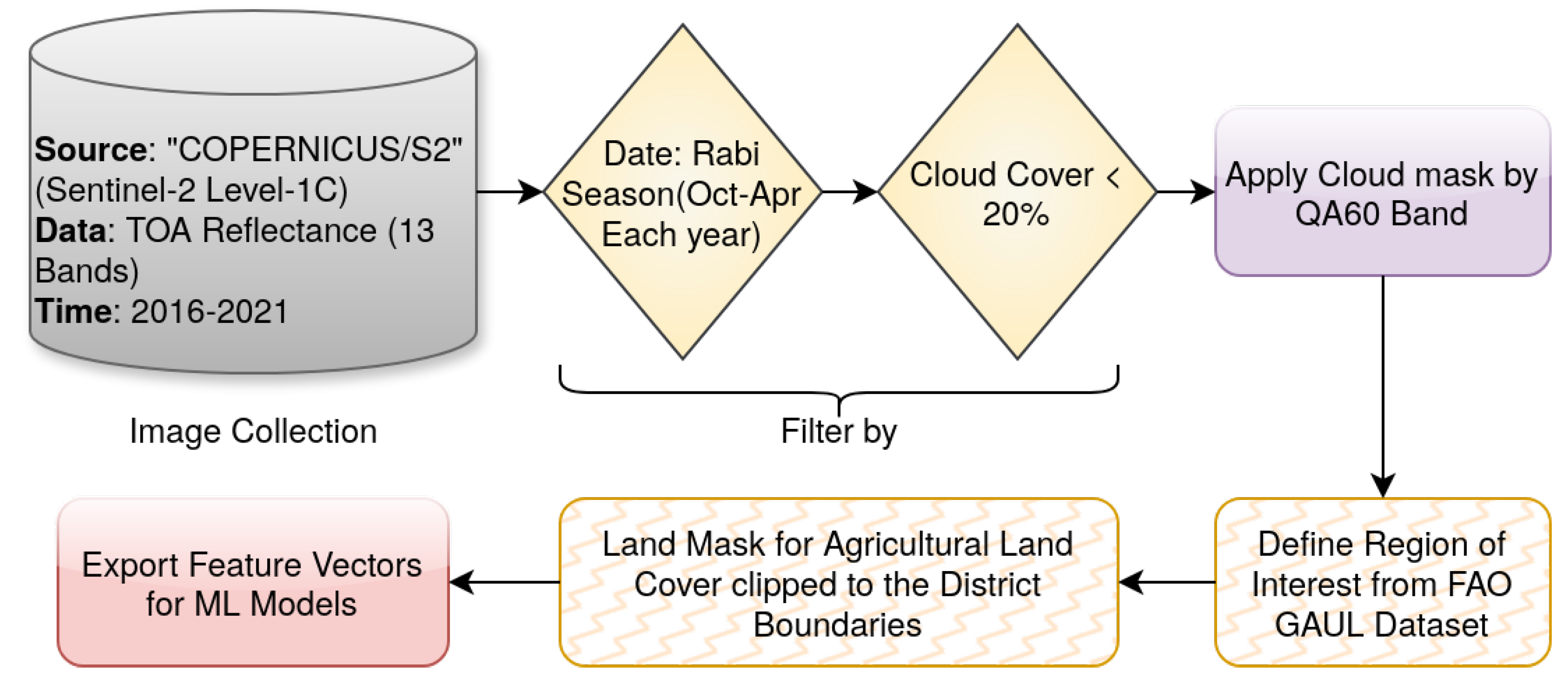
Figure 21.
Model Aggregation for 5 most relevant features before Oversampling.
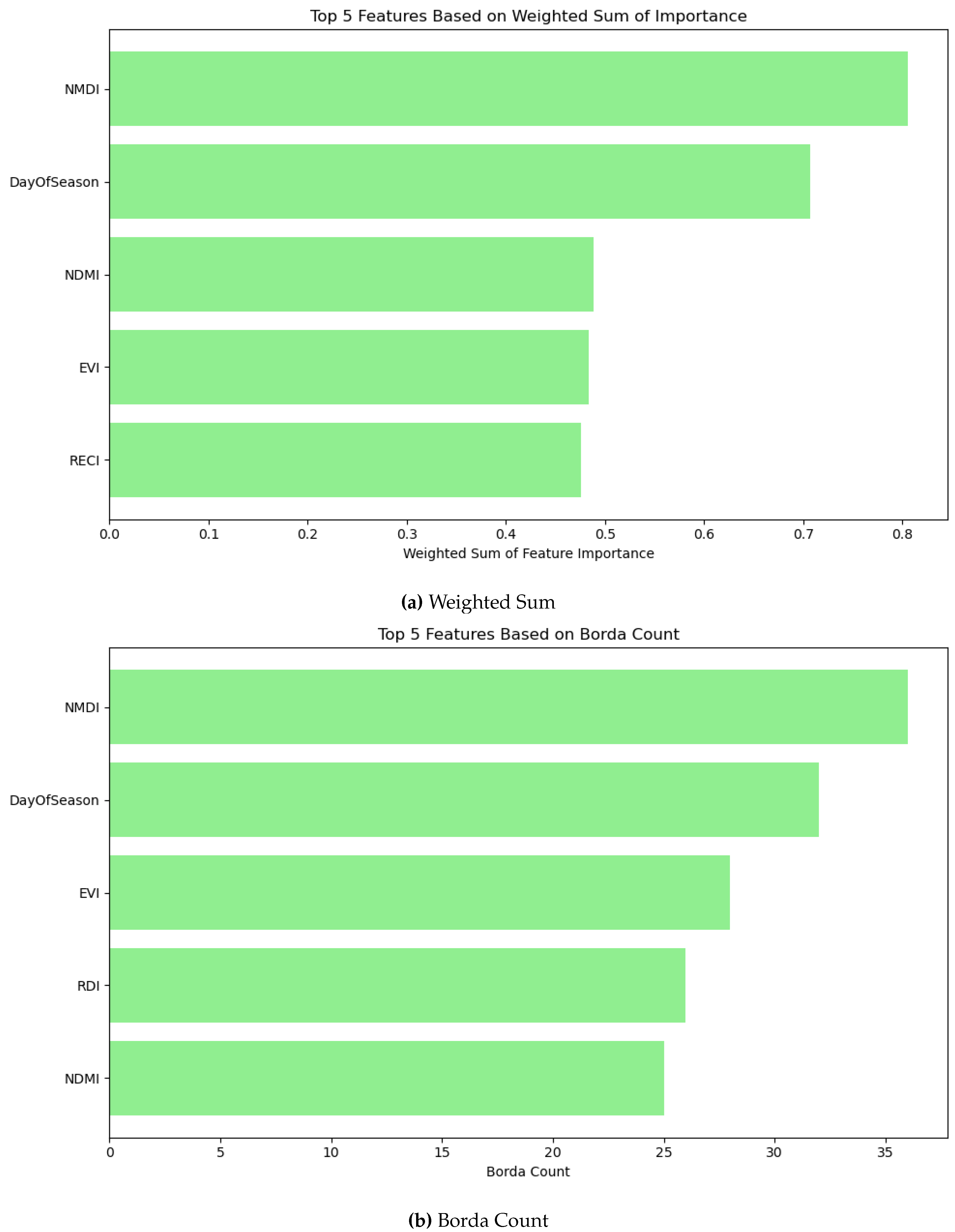
Figure 23.
Model Aggregation for 5 most relevant features in Borderline SMOTE.
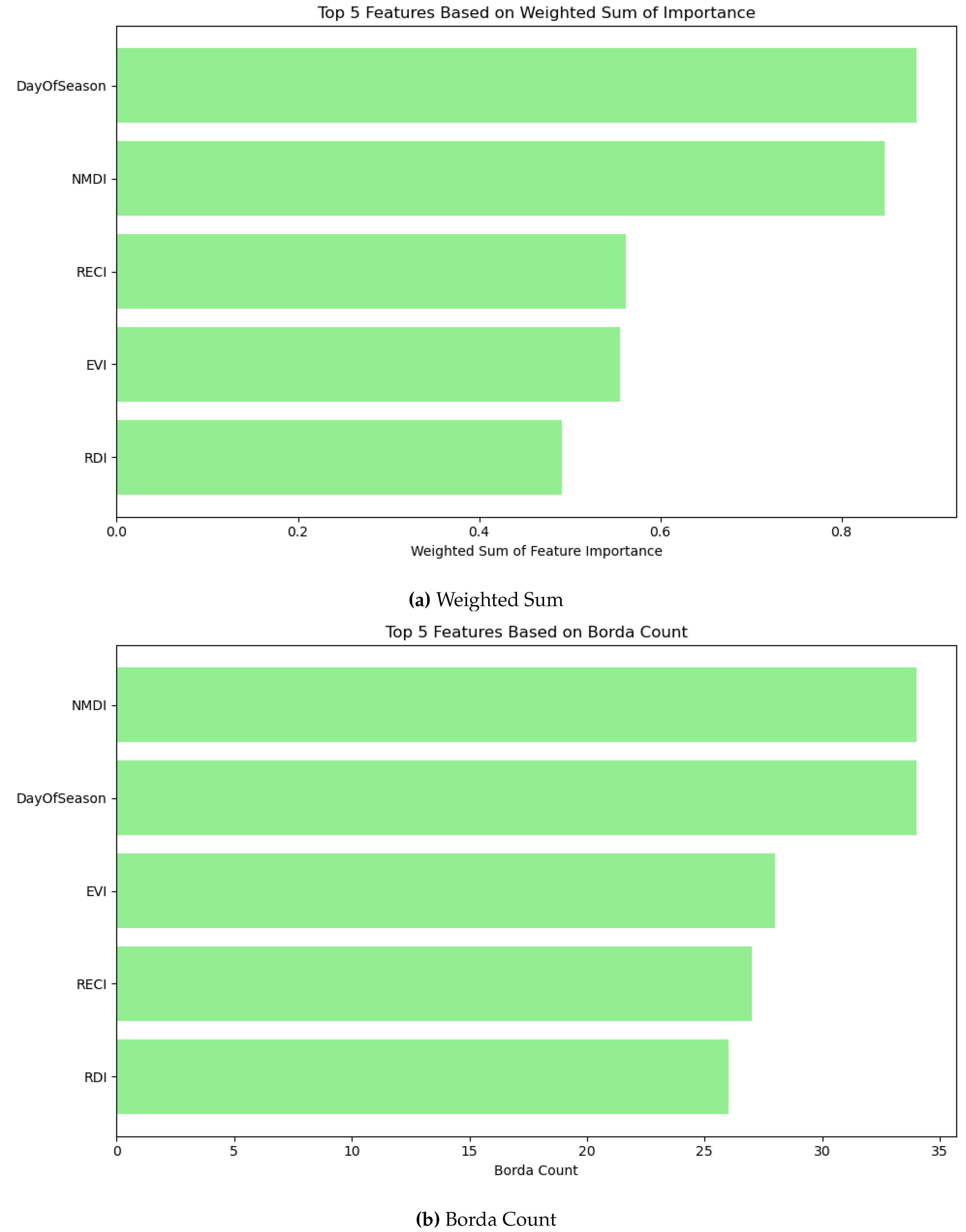
Table 1.
Part of the Exported Data Set from TimeSeries data of Amravati in 2018.
| ARVI | EVI | MNDVI | MNDWI | NDMI | NDVI | NDWI | NMDI | RDI | RECI | SAVI | TVI | date |
|---|---|---|---|---|---|---|---|---|---|---|---|---|
| 0.2713 | 0.4561 | -0.2863 | -0.2797 | -0.0222 | 0.2668 | -0.2600 | 0.4326 | 1.8608 | 0.5180 | 0.4802 | 0.8747 | 2018-01-02 |
| 0.2912 | 0.6662 | -0.3054 | -0.3240 | -0.0341 | 0.2881 | -0.2937 | 0.4220 | 1.9493 | 0.5633 | 0.5184 | 0.8864 | 2018-01-07 |
| 0.2950 | 0.7153 | -0.3604 | -0.3653 | -0.0481 | 0.2945 | -0.3228 | 0.4089 | 2.2248 | 0.6098 | 0.5299 | 0.8894 | 2018-01-17 |
Table 2.
Sample data of district-specific responses over the years.
| Year/District | Jodhpur | Amravati | Thanjavur |
|---|---|---|---|
| 2016 | Drought | Drought | No Drought |
| 2017 | No Drought | No Drought | Drought |
| 2018 | No Drought | No Drought | No Drought |
| 2019 | Drought | Drought | Drought |
| 2020 | Drought | No Drought | No Drought |
| 2021 | No Drought | No Drought | No Drought |
Table 3.
Before Oversampling: Comparison of classification methods based on Accuracy, Precision, and Recall.
Table 3.
Before Oversampling: Comparison of classification methods based on Accuracy, Precision, and Recall.
| Methods/Metrics | Accuracy | Precision | Recall |
|---|---|---|---|
| XG Boost | 0.8230 | 0.7982 | 0.7390 |
| Random Forest | 0.8339 | 0.8349 | 0.7225 |
| Bagging Classifier | 0.8415 | 0.8344 | 0.7473 |
| Gradient Boosting | 0.7459 | 0.7500 | 0.5457 |
Table 4.
SMOTE: Comparison of classification methods based on Accuracy, Precision, and Recall.
| Methods/Metrics | Accuracy | Precision | Recall |
|---|---|---|---|
| XG Boost | 0.7937 | 0.7112 | 0.8049 |
| Random Forest | 0.7861 | 0.7002 | 0.8022 |
| Bagging Classifier | 0.7807 | 0.6966 | 0.7875 |
| Gradient Boosting | 0.7090 | 0.6062 | 0.7527 |
Table 5.
Borderline SMOTE: Comparison of classification methods based on Accuracy, Precision, and Recall.
Table 5.
Borderline SMOTE: Comparison of classification methods based on Accuracy, Precision, and Recall.
| Methods/Metrics | Accuracy | Precision | Recall |
|---|---|---|---|
| XG Boost | 0.8393 | 0.8426 | 0.7527 |
| Random Forest | 0.8426 | 0.8544 | 0.7253 |
| Bagging Classifier | 0.8371 | 0.8344 | 0.7335 |
| Gradient Boosting | 0.7286 | 0.6667 | 0.6264 |
Table 7.
Confusion Matrix - Before Oversampling.
| (a) XGBoost | ||
|---|---|---|
| Predicted | ||
| Actual | No Drought | Drought |
| No Drought | 489 | 68 |
| Drought | 95 | 269 |
| (b) Random Forest | ||
| Predicted | ||
| Actual | No Drought | Drought |
| No Drought | 505 | 52 |
| Drought | 101 | 263 |
| (c) Bagging | ||
| Predicted | ||
| Actual | No Drought | Drought |
| No Drought | 503 | 54 |
| Drought | 92 | 272 |
| (d) Gradient Boosting | ||
| Predicted | ||
| Actual | No Drought | Drought |
| No Drought | 492 | 65 |
| Drought | 169 | 195 |
Table 8.
Confusion Matrix - Oversampling with SMOTE.
| (a) XGBoost | ||
|---|---|---|
| Predicted | ||
| Actual | No Drought | Drought |
| No Drought | 438 | 119 |
| Drought | 71 | 293 |
| (b) Random Forest | ||
| Predicted | ||
| Actual | No Drought | Drought |
| No Drought | 432 | 125 |
| Drought | 72 | 292 |
| (c) Bagging | ||
| Predicted | ||
| Actual | No Drought | Drought |
| No Drought | 432 | 125 |
| Drought | 77 | 287 |
| (d) Gradient Boosting | ||
| Predicted | ||
| Actual | No Drought | Drought |
| No Drought | 379 | 178 |
| Drought | 90 | 274 |
Table 9.
Confusion Matrix - Oversampling with Borderline SMOTE
| (a) XGBoost | ||
|---|---|---|
| Predicted | ||
| Actual | No Drought | Drought |
| No Drought | 499 | 58 |
| Drought | 90 | 274 |
| (b) Random Forest | ||
| Predicted | ||
| Actual | No Drought | Drought |
| No Drought | 512 | 45 |
| Drought | 100 | 264 |
| (c) Bagging | ||
| Predicted | ||
| Actual | No Drought | Drought |
| No Drought | 504 | 53 |
| Drought | 97 | 267 |
| (d) Gradient Boosting | ||
| Predicted | ||
| Actual | No Drought | Drought |
| No Drought | 443 | 114 |
| Drought | 136 | 228 |
Table 10.
Confusion Matrix - Oversampling with ADASYN.
| (a) XGBoost | ||
|---|---|---|
| Predicted | ||
| Actual | No Drought | Drought |
| No Drought | 475 | 82 |
| Drought | 63 | 301 |
| (b) Random Forest | ||
| Predicted | ||
| Actual | No Drought | Drought |
| No Drought | 473 | 84 |
| Drought | 61 | 303 |
| (c) Bagging | ||
| Predicted | ||
| Actual | No Drought | Drought |
| No Drought | 475 | 82 |
| Drought | 72 | 292 |
| (d) Gradient Boosting | ||
| Predicted | ||
| Actual | No Drought | Drought |
| No Drought | 388 | 169 |
| Drought | 91 | 273 |
Table 11.
Group-wise Before Oversampling: Comparison of classification methods based on Accuracy, Precision, and Recall.
Table 11.
Group-wise Before Oversampling: Comparison of classification methods based on Accuracy, Precision, and Recall.
| Methods/Metrics | Accuracy | Precision | Recall |
|---|---|---|---|
| XG Boost | 0.94 | 0.94 | 0.94 |
| Random Forest | 0.94 | 0.94 | 0.94 |
| Bagging Classifier | 0.94 | 0.94 | 0.94 |
| Gradient Boosting | 0.83 | 0.83 | 0.83 |
Table 12.
Group-wise SMOTE: Comparison of classification methods based on Accuracy, Precision, and Recall.
Table 12.
Group-wise SMOTE: Comparison of classification methods based on Accuracy, Precision, and Recall.
| Methods/Metrics | Accuracy | Precision | Recall |
|---|---|---|---|
| XG Boost | 0.94 | 0.94 | 0.94 |
| Random Forest | 0.88 | 0.88 | 0.88 |
| Bagging Classifier | 0.94 | 0.94 | 0.94 |
| Gradient Boosting | 0.83 | 0.83 | 0.83 |
Table 13.
Group-wise Borderline SMOTE: Comparison of classification methods based on Accuracy, Precision, and Recall.
Table 13.
Group-wise Borderline SMOTE: Comparison of classification methods based on Accuracy, Precision, and Recall.
| Methods/Metrics | Accuracy | Precision | Recall |
|---|---|---|---|
| XG Boost | 0.94 | 0.94 | 0.94 |
| Random Forest | 0.94 | 0.94 | 0.94 |
| Bagging Classifier | 0.94 | 0.94 | 0.94 |
| Gradient Boosting | 0.94 | 0.94 | 0.94 |
Table 14.
Group-wise ADASYN: Comparison of classification methods based on Accuracy, Precision, and Recall.
Table 14.
Group-wise ADASYN: Comparison of classification methods based on Accuracy, Precision, and Recall.
| Methods/Metrics | Accuracy | Precision | Recall |
|---|---|---|---|
| XG Boost | 1.00 | 1.00 | 1.00 |
| Random Forest | 1.00 | 1.00 | 1.00 |
| Bagging Classifier | 1.00 | 1.00 | 1.00 |
| Gradient Boosting | 0.89 | 0.89 | 0.89 |
Table 15.
Model performance of Top 1 to Top 5 feature using Weighted Sum before overampling.
| XGBoost | Random Forest | Bagging | Gradient Boosting | |
|---|---|---|---|---|
| Top 1 | Acc: 0.6253 Prec: 0.5493 Rec: 0.3797 |
Acc: 0.6015 Prec: 0.4959 Rec: 0.4973 |
Acc: 0.6004 Prec: 0.495 Rec: 0.4945 |
Acc: 0.6352 Prec: 0.6111 Rec: 0.2115 |
| Top 2 | Acc: 0.734 Prec: 0.6951 Rec: 0.5824 |
Acc: 0.709 Prec: 0.6463 Rec: 0.5824 |
Acc: 0.6916 Prec: 0.5615 Rec: 0.5852 |
Acc: 0.658 Prec: 0.6485 Rec: 0.3295 |
| Top 3 | Acc: 0.747 Prec: 0.7191 Rec: 0.5097 |
Acc: 0.7633 Prec: 0.7548 Rec: 0.6297 |
Acc: 0.7644 Prec: 0.7139 Rec: 0.6374 |
Acc: 0.7025 Prec: 0.7308 Rec: 0.3486 |
| Top 4 | Acc: 0.7894 Prec: 0.7656 Rec: 0.6731 |
Acc: 0.7752 Prec: 0.7041 Rec: 0.6648 |
Acc: 0.7687 Prec: 0.7382 Rec: 0.6297 |
Acc: 0.7188 Prec: 0.7465 Rec: 0.3486 |
| Top 5 | Acc: 0.81 Prec: 0.7936 Rec: 0.7033 |
Acc: 0.81 Prec: 0.7981 Rec: 0.6951 |
Acc: 0.7894 Prec: 0.7607 Rec: 0.6813 |
Acc: 0.7318 Prec: 0.7352 Rec: 0.4239 |
Table 16.
Model performance of Top 1 to Top 5 feature using Borda Count before oversamping.
| XGBoost | Random Forest | Bagging | Gradient Boosting | |
|---|---|---|---|---|
| Top 1 | Acc: 0.625 Prec: 0.549 Rec: 0.3797 |
Acc: 0.6015 Prec: 0.4959 Rec: 0.4973 |
Acc: 0.6004 Prec: 0.495 Rec: 0.4945 |
Acc: 0.6352 Prec: 0.6111 Rec: 0.2115 |
| Top 2 | Acc: 0.734 Prec: 0.6951 Rec: 0.5824 |
Acc: 0.709 Prec: 0.6463 Rec: 0.5824 |
Acc: 0.6916 Prec: 0.5615 Rec: 0.5852 |
Acc: 0.658 Prec: 0.6485 Rec: 0.3295 |
| Top 3 | Acc: 0.7492 Prec: 0.7152 Rec: 0.6701 |
Acc: 0.7416 Prec: 0.7019 Rec: 0.6016 |
Acc: 0.7362 Prec: 0.685 Rec: 0.6164 |
Acc: 0.6721 Prec: 0.6722 Rec: 0.3324 |
| Top 4 | Acc: 0.7991 Prec: 0.7573 Rec: 0.6521 |
Acc: 0.7894 Prec: 0.7591 Rec: 0.6841 |
Acc: 0.785 Prec: 0.7496 Rec: 0.6293 |
Acc: 0.6938 Prec: 0.6667 Rec: 0.4052 |
| Top 5 | Acc: 0.8241 Prec: 0.8079 Rec: 0.7083 |
Acc: 0.8263 Prec: 0.8282 Rec: 0.7143 |
Acc: 0.8208 Prec: 0.7953 Rec: 0.7363 |
Acc: 0.7318 Prec: 0.7362 Rec: 0.3987 |
Table 17.
Model performance of Top 1 to Top 5 feature using Weighted Sum in SMOTE.
| XGBoost | Random Forest | Bagging | Gradient Boosting | |
|---|---|---|---|---|
| Top 1 | Acc: 0.6428 Prec: 0.5368 Rec: 0.7005 |
Acc: 0.6384 Prec: 0.5324 Rec: 0.7005 |
Acc: 0.6384 Prec: 0.5324 Rec: 0.7005 |
Acc: 0.5863 Prec: 0.4827 Rec: 0.6511 |
| Top 2 | Acc: 0.6960 Prec: 0.5933 Rec: 0.7335 |
Acc: 0.6743 Prec: 0.5714 Rec: 0.7033 |
Acc: 0.6775 Prec: 0.5743 Rec: 0.7115 |
Acc: 0.6308 Prec: 0.5241 Rec: 0.717 |
| Top 3 | Acc: 0.7481 Prec: 0.6454 Rec: 0.8049 |
Acc: 0.7622 Prec: 0.6706 Rec: 0.7830 |
Acc: 0.7611 Prec: 0.6651 Rec: 0.7967 |
Acc: 0.6417 Prec: 0.5381 Rec: 0.6593 |
| Top 4 | Acc: 0.7731 Prec: 0.6850 Rec: 0.7885 |
Acc: 0.7785 Prec: 0.6914 Rec: 0.7940 |
Acc: 0.7763 Prec: 0.6946 Rec: 0.7747 |
Acc: 0.6743 Prec: 0.5711 Rec: 0.7060 |
| Top 5 | Acc: 0.7742 Prec: 0.6912 Rec: 0.7747 |
Acc: 0.7600 Prec: 0.6706 Rec: 0.7720 |
Acc: 0.7633 Prec: 0.6722 Rec: 0.7830 |
Acc: 0.6667 Prec: 0.5621 Rec: 0.7088 |
Table 18.
Model performance of Top 1 to Top 5 feature using Borda Count in SMOTE.
| XGBoost | Random Forest | Bagging | Gradient Boosting | |
|---|---|---|---|---|
| Top 1 | Acc: 0.5559 Prec: 0.4592 Rec: 0.6951 |
Acc: 0.5668 Prec: 0.4635 Rec: 0.6099 |
Acc: 0.5668 Prec: 0.4635 Rec: 0.6099 |
Acc: 0.5559 Prec: 0.4624 Rec: 0.7610 |
| Top 2 | Acc: 0.6960 Prec: 0.5933 Rec: 0.7335 |
Acc: 0.6797 Prec: 0.5762 Rec: 0.7170 |
Acc: 0.6786 Prec: 0.5756 Rec: 0.7115 |
Acc: 0.6308 Prec: 0.5241 Rec: 0.7170 |
| Top 3 | Acc: 0.7090 Prec: 0.6127 Rec: 0.7170 |
Acc: 0.7101 Prec: 0.6131 Rec: 0.7225 |
Acc: 0.7123 Prec: 0.6187 Rec: 0.7008 |
Acc: 0.6482 Prec: 0.5379 Rec: 0.7802 |
| Top 4 | Acc: 0.7535 Prec: 0.6546 Rec: 0.7967 |
Acc: 0.7427 Prec: 0.6440 Rec: 0.7802 |
Acc: 0.7459 Prec: 0.6540 Rec: 0.7582 |
Acc: 0.6721 Prec: 0.5671 Rec: 0.7198 |
| Top 5 | Acc: 0.7828 Prec: 0.6981 Rec: 0.7940 |
Acc: 0.7655 Prec: 0.6762 Rec: 0.7802 |
Acc: 0.7546 Prec: 0.6612 Rec: 0.7775 |
Acc: 0.6667 Prec: 0.5621 Rec: 0.7088 |
Table 19.
Model performance of Top 1 to Top 5 feature using Weighted Sum in Borderline Smote.
| XGBoost | Random Forest | Bagging | Gradient Boosting | |
|---|---|---|---|---|
| Top 1 | Acc: 0.6602 Prec: 0.5770 Rec: 0.5247 |
Acc: 0.6721 Prec: 0.5901 Rec: 0.5577 |
Acc: 0.6634 Prec: 0.5734 Rec: 0.5797 |
Acc: 0.6580 Prec: 0.6052 Rec: 0.3874 |
| Top 2 | Acc: 0.7177 Prec: 0.6615 Rec: 0.5852 |
Acc: 0.7144 Prec: 0.6583 Rec: 0.5769 |
Acc: 0.6873 Prec: 0.6111 Rec: 0.5742 |
Acc: 0.6754 Prec: 0.6148 Rec: 0.4780 |
| Top 3 | Acc: 0.7524 Prec: 0.7208 Rec: 0.6099 |
Acc: 0.7622 Prec: 0.7393 Rec: 0.6154 |
Acc: 0.7568 Prec: 0.7273 Rec: 0.6154 |
Acc: 0.6992 Prec: 0.6445 Rec: 0.5330 |
| Top 4 | Acc: 0.7644 Prec: 0.7348 Rec: 0.6319 |
Acc: 0.7524 Prec: 0.7208 Rec: 0.6099 |
Acc: 0.7524 Prec: 0.7166 Rec: 0.6181 |
Acc: 0.6862 Prec: 0.6106 Rec: 0.5687 |
| Top 5 | Acc: 0.8122 Prec: 0.8091 Rec: 0.6868 |
Acc: 0.8165 Prec: 0.8155 Rec: 0.6923 |
Acc: 0.8176 Prec: 0.8182 Rec: 0.6923 |
Acc: 0.6840 Prec: 0.6034 Rec: 0.5852 |
Table 20.
Model performance of Top 1 to Top 5 feature using Borda Count in Borderline Smote.
| XGBoost | Random Forest | Bagging | Gradient Boosting | |
|---|---|---|---|---|
| Top 1 | Acc: 0.5820 Prec: 0.4673 Rec: 0.4121 |
Acc: 0.5896 Prec: 0.4834 Rec: 0.5604 |
Acc: 0.5896 Prec: 0.4834 Rec: 0.5604 |
Acc: 0.6135 Prec: 0.5153 Rec: 0.3709 |
| Top 2 | Acc: 0.7177 Prec: 0.6615 Rec: 0.5852 |
Acc: 0.7199 Prec: 0.6688 Rec: 0.5769 |
Acc: 0.6851 Prec: 0.6088 Rec: 0.5687 |
Acc: 0.6754 Prec: 0.6148 Rec: 0.4780 |
| Top 3 | Acc: 0.7275 Prec: 0.6707 Rec: 0.6099 |
Acc: 0.7329 Prec: 0.6903 Rec: 0.5879 |
Acc: 0.7090 Prec: 0.6472 Rec: 0.5797 |
Acc: 0.6667 Prec: 0.5893 Rec: 0.5165 |
| Top 4 | Acc: 0.7514 Prec: 0.7116 Rec: 0.6236 |
Acc: 0.7535 Prec: 0.7231 Rec: 0.6099 |
Acc: 0.7293 Prec: 0.7152 Rec: 0.6071 |
Acc: 0.6873 Prec: 0.6105 Rec: 0.5769 |
| Top 5 | Acc: 0.8078 Prec: 0.7877 Rec: 0.7033 |
Acc: 0.8143 Prec: 0.8123 Rec: 0.6886 |
Acc: 0.8154 Prec: 0.8129 Rec: 0.7775 |
Acc: 0.6667 Prec: 0.5621 Rec: 0.6923 |
Disclaimer/Publisher’s Note: The statements, opinions and data contained in all publications are solely those of the individual author(s) and contributor(s) and not of MDPI and/or the editor(s). MDPI and/or the editor(s) disclaim responsibility for any injury to people or property resulting from any ideas, methods, instructions or products referred to in the content. |
© 2025 by the authors. Licensee MDPI, Basel, Switzerland. This article is an open access article distributed under the terms and conditions of the Creative Commons Attribution (CC BY) license (http://creativecommons.org/licenses/by/4.0/).
Copyright: This open access article is published under a Creative Commons CC BY 4.0 license, which permit the free download, distribution, and reuse, provided that the author and preprint are cited in any reuse.


