
Submitted:
02 September 2025
Posted:
03 September 2025
You are already at the latest version
Abstract
Meteorological drought is characterized by both magnitude and duration, and its spatiotemporal dynamics drive its propagation to other drought type. Ethiopia’s agricultural sector faces significant challenges in achieving accurate crop yield prediction, a critical requirement for effective resource management and ensuring food security for its rapidly growing population. This study analyzes drought propagation dynamics across Ethiopia for 1981-2022 period and their impacts on cereal crop yields-maize, sorghum teff and wheat over 1993-2022. Multi-scale meteorological drought indices (SPI, SPEI at 1-12 months) from observed and ENACT rainfall and temperature data were integrated with root-zone soil moisture anomalies to map spatio-temporal propagation. Lagged correlation and maximum-correlation lag times quantified lead times between meteorological and soil moisture droughts. Random Forest and XGBoost models were applied for yield prediction, evaluated using RMSE and R2. Results indicate spatially variable drought regimes, with rapid onset in lowlands and slow cumulative patterns in highlands, alongside crop specific vulnerability periods. Maximum temperature and medium-term drought consistently dominated as predictors, highlighting combined heat and moisture stress effects. Recommended adaptation include breeding for heat-tolerant maize and wheat, implementing water-saving agronomy and supplemental irrigation, adjusting planting dates to avoid peak heat, and diversifying cropping systems to mitigate climate risks.
Keywords:
cereal crop yield prediction
; drought propagation dynamics
; food security in sub‐saharan Africa
; meteorological drought
; soil drought
; random forest
; Ethiopia
Abstract
Meteorological drought is characterized by both magnitude and duration, and its spatiotemporal dynamics drive its propagation to other drought type. Ethiopia’s agricultural sector faces significant challenges in achieving accurate crop yield prediction, a critical requirement for effective resource management and ensuring food security for its rapidly growing population. This study analyzes drought propagation dynamics across Ethiopia for 1981-2022 period and their impacts on cereal crop yields-maize, sorghum teff and wheat over 1993-2022. Multi-scale meteorological drought indices (SPI, SPEI at 1-12 months) from observed and ENACT rainfall and temperature data were integrated with root-zone soil moisture anomalies to map spatio-temporal propagation. Lagged correlation and maximum-correlation lag times quantified lead times between meteorological and soil moisture droughts. Random Forest and XGBoost models were applied for yield prediction, evaluated using RMSE and R2. Results indicate spatially variable drought regimes, with rapid onset in lowlands and slow cumulative patterns in highlands, alongside crop specific vulnerability periods. Maximum temperature and medium-term drought consistently dominated as predictors, highlighting combined heat and moisture stress effects. Recommended adaptation include breeding for heat-tolerant maize and wheat, implementing water-saving agronomy and supplemental irrigation, adjusting planting dates to avoid peak heat, and diversifying cropping systems to mitigate climate risks.
1. Introduction
Drought is a complex, extreme and prolonged natural disaster triggered by below-normal rainfall over a period of months to years, and resulting in costly and destructive impacts on lives and livelihood of a nations [1]. This complex recurrent disaster characterized by its severity, duration and spatial extent, which is known as a creeping phenomenon, making an accurate prediction of either its onset or end date is a challenging. Because its length is highly variable starting from few weeks to several years, encompassing wide spatial ranges [2]. Accordingly, drought is a temporary dry period due to below normal rainfall, whereas the aridity is a continuous dryness where the amount of moisture is highly dependent on potential evapotranspiration [3]. On the other hand, the arid agro-ecology zone suffers from serious moisture stress, thus, highly prone to drought, because annual mean potential evapotranspiration exceeds annual mean rainfall [4]. Moreover, the rate of changes in potential evapotranspiration is consistently increasing, while the rate of change in rainfall is highly fluctuates in both temporal and spatial pattern under global warming [5].
Although drought progresses more slowly than other natural disasters, it is a severe weather event caused by a lack of rain or an imbalance between the availability of water and its usage for various activities [6]. As a result, drought tends to affect large areas for extended periods. At present, it is considered one of the most destructive natural calamities because of the significant harm it is causing. In addition, drought can greatly affect farming, the safety of water resources, the environment, and economic progress by worsening the lack of moisture in the soil [7]. Thus, to improve efforts for resisting and dealing with drought, it is essential to strengthen monitoring activities for drought and carry out in-depth research on patterns related to drought.
In recent years, under the coupled influence of global warming and intensified environmental degradation, the scope of multi-type droughts are broadened with more frequent and widespread occurrence [8]. Along equatorial regions, failure or shortage of rainfall is caused by a persistent anomalies in large-scale atmospheric circulation which is often triggered by anomalous tropical sea surface temperatures (SSTs), or by other teleconnections [9]. Local feedbacks of land-atmosphere, with underlying environmental conditions and high temperatures often enhance the atmospheric anomalies [10]. According to the World Meteorological Organization (WMO) report, there are four types of drought namely meteorological drought, hydrological drought agricultural drought and socioeconomic drought, respectively [11]. Typically, a long stretch and below normal rain is the main reason for meteorological drought, marking the first phase in the onset of a drought situation. When rainfall falls below a certain threshold, meteorological drought occurs first, followed by a decrease in runoff and soil moisture, triggering hydrological drought and agricultural drought, both of which can have an impact on water supply and crop production, eventually leading to socioeconomic drought [12]. Therefore, drought propagation refers to a process by which drought conditions transfer from the atmosphere to soil moisture and river systems [13]. Thus, it is essential to explore drought propagation mechanism, how various droughts reacts to meteorological drought [14].
Drought propagation is defined as the transmission of signals about moisture deficits between various types of drought, such as the shift from meteorological drought to agricultural/hydrological drought [15]. The causes of meteorological/hydrological drought are intricate, as they are contingent on both the atmosphere and the hydrological processes that supply moisture to the atmosphere and cause water storage and runoff to stream [16]. Climatic variability is the cause of the atmospheric processes that initiate the development of agricultural and hydrological drought. Soil moisture storage depletion is linked to its previous condition, drainage into the groundwater, and evapotranspiration from bare soil, especially from vegetation. Potential evapotranspiration might rise throughout a dry spell as a result of increased radiation, temperature, and decreased moisture availability. As a result, real evapotranspiration may increase, which might cause more water to be lost from the soil and open water sources. Extreme drought can restrict evapotranspiration by restricting the availability of soil moisture and causing plants to witting, thereby reducing future soil moisture depletion but also perhaps limiting local rainfall production, which contributes to the persistence of drought conditions. According to some authors, vegetation is a crucial component in changing these feedbacks [17]. Drought spreads throughout the hydrological cycle, moving between various sorts, including spatial occurrence, development, recovery, and transmission. In recent years, there is a lot of focus on spatial and temporal continuity studies of drought [18]. Accordingly, drought propagation is strongly associated to climate types and seasonality, occurring at sub-seasonal timescales in tropical climates and at up to multi-annual timescales in arid climates [19].
Drought prevalence (intensity, frequency and duration) is highly linked with large-scale ocean-atmospheric teleconnection across tropical regions [20]. El Niño and La Niña are Pacific Ocean-based meteorological phenomena that have the potential to significantly affect worldwide weather patterns, particularly across tropical regions [21]. Analysis of large-scale ocean-atmospheric teleconnection suggest that the inverse relationship between El Niño-Southern oscillation (ENSO) and anomalous rainfall occurrence across Ethiopia, resulting in devastating drought. This is because southeastward shift in the Walker circulation anomalies associated with ENSO events might lead to a reduced subsidence over Ethiopia [22]. In Ethiopia, there is a strong correlation between drought occurrence and the ENSO phenomenon. As an example, the catastrophic drought of 2022 [23], and the widespread drought of 2015 that affected all of Ethiopia's districts are categorized as food insecure, leading to a scarcity of water for people and animals [24]. According to certain writers, between 50% and 80% of the total annual rainfall in Ethiopia occurs during the summer season, which lasts from June through September (JJAS) [25]. This demonstrates the effect of the JJAS rain on the nation's mainly agricultural economy is significant. El Niño event is one of the primary causes of the fluctuations in rainfall during the Ethiopian summer [26]. However, the aforementioned research and other researchers have only concentrated on the connection between ENSO and drought conditions and have failed to account for its interactions with different climate zones throughout Ethiopia. Consequently, the focus of this research is on the relationship between Ethiopian climate regions (arid, semiarid, sub-humid, and humid) with ENSO events.
Agricultural drought results from insufficient rainfall, leading to the deaths of more than 10 million individuals and economic losses amounting to hundreds of billions of dollars [7]. A study of literature from Africa country indicated that drought has devastating impacts, leading to 33% reduction in grazing land, 17% decrease in water, poor water quality and availability, and 11% loss of vegetation coverage [27]. Additionally, evidence shows that the number of livestock declined by 15%, drop in crop yields by 8. 4% [28]. Ethiopia has a history of being one of the countries that suffers the most from climate-related disasters, especially droughts, due to rainfall deficit during the rainy season. The World Meteorological Organization report states that the drought of 1983/84 is caused 300,000 fatalities, while the 1973 drought led to 100,100 deaths and the 2015 drought resulted in economic losses totaling 1.48 billion US dollars [29]. As reported by the United Nations Office for the Coordination of Humanitarian Affairs (OCHA), 24.1 million people are affected, resulting in economic losses of 16.99 million US dollars as a consequence of 2022 drought [30].
A comprehensive identification of drought propagation is crucial for risk mitigation and forecasting efforts. While studies highlight the cascading impacts of drought propagation, significant gaps remain in comprehending the multiscale spatio-temporal dynamics and soil depth-dependent response. For instance, some scholars have investigated drought events by constructing a multi-varieties drought index by simultaneously representing meteorological and hydrological droughts to show drought propagation in the catchment area in southern Ethiopia [31]. Similarly, the prevalence of drought and its impact on crop production at district level is analyzed to show spatio-temporal occurrence and influence on crop production [32]. However, there is a limited study on drought propagation dynamics in different agro-climate zone, agricultural yield predictions using machine leering models, and the predictive potential of different models. Drought propagation is linked to variations in anomalies of large-scale atmospheric circulation signals, thus, drought disrupts the interrelated links of hydrological cycles [33]. Several features, including the timing of successive stages of drought, such as frequency, intensity, and length, may change as a result of these processes [34]. Identifying the dominant driving forces is critical for drought prediction and monitoring. Further exploring the possible driving factors of drought and the associated agricultural production is of great practical significance for revealing the formation mechanisms of drought, formulating reasonable drought-relief measures, ensuring food security and maintaining social stability [33]. Understanding the variables that cause drought, the spatial and temporal dynamics of how it spreads across various types, and how it affects agricultural production could help us to take preventative steps to minimize crop losses. In order to fill the aforementioned research gaps, this study seeks to examine spatiotemporal drought propagation dynamics as well as critical driving variables of drought and associated agricultural production.
Statistical methods analyze drought transition time by building relationship between drought characteristics of different types of events. Correlation analysis, Multi-linear regression, and principal component analysis are examples of empirical statistical methods that are useful for assessing the linkage of driving forces [35]. However, drought-causing mechanisms do not always fit the basic linear model, drivers could have linkage with one another [36]. As a result, empirical statistical approaches would produce results that are contrary to reality. Because of their great accuracy, machine learning algorithms are recently showed widespread success in attribution evaluation. Popular non-parametric techniques for attribution analysis include tree-based machine learning models like XGBoosting (XGB) and Random Forest regression (RF) [37]. It is also found that machine learning models could construct a nonlinear link between drivers and their related parameters, as well as identify the key causes of drought propagation. Furthermore, interpretable machine learning models offer a useful method for intricate link between physical quantities [37]. To enhance the accuracy of agricultural yield prediction, various machine learning approaches are investigated. This study primary concentrates on XGB and RF which are applied to predict the yield of cereal crops, which aids farmers in choosing and cultivating the most economical crops across Ethiopia, which lowers the likelihood of loss and raising the value of farming land. For example, [38], discussed the significance of crop yield prediction, and stated that it is crucial for efficient crop management, sustainable agriculture and food security. Thus, this research aims to investigate spatio-temporal drought propagation dynamics, and cereal crop yield production using machine learning models under global warming. Specifically, the following objectives are designed:
- ✓ To analyze the spatio-temporal pattern of meteorological drought occurrence in different climate regions across Ethiopia.
- ✓ To analyze the response of agricultural drought to meteorological drought, and discuss drought propagation dynamics at different climate zones in Ethiopia.
- ✓ To evaluate the predictive potential of machine learning models and feature importance in predicting cereal crop yields.
2. Methodology
2.1. Study Area
Astronomically, Ethiopia is located in the Horn of Africa inside 3oN to 15oN and 330E to 48oE (Fig), bordered with Eritrea to the north, Djibouti to the east, Sudan to the west, Kenya to the south, and Somalia to the south and east [22]. It covers an area of about 1.14 million square kilometres, and the country’s topography consists of high and rugged plateaus and the peripheral lowlands [39]. The lowest and highest points in Ethiopia are 4534 m above mean sea level and 231 m below mean sea level (Figure 1a). This vast irregularity in topography creates varying rainfall regimes with annual total of 84-345 mm in the south-eastern and north-eastern, 1155-2137 mm in the south-western and central part of a country (Figure 1b).
Aridity is often expressed as a generalized function of rainfall and potential evapotranspiration (PET), is the ratio of annual mean rainfall (MAP) to mean annual potential evapotranspiration. It is a moisture available in relation to atmospheric water demand, and quantifies water availability for plant growth and development, comparing incoming moisture totals with potential out-going moisture. According to this expression, Aridity Index (AI) map for different climate zone in Ethiopia is generated covering the years 1981 to 2022 (Figure 1c). It is used to show the dependency of soil moisture on dry-wet conditions under varying climatic conditions, climate classification utilizes the Global Aridity Index (AI) provided by the Consultative Group on International Agricultural Research Consortium for Spatial Information (CGIAR) [40]. This index is utilized to categorize areas into hyper-arid (AI<0.03), arid (0.032<AI<0.02), semi-arid (0.02<AI<0.5), sub-humid (0.5<AI<0.65), and humid (AI>0.65) classifications [41]. To better understand how drought propagates and why there are differences across regions, Ethiopia is divided into specific zones based on AI. These include humid, semi-humid, arid, semi-arid and hyper-arid zones. Furthermore, regions that receive less than 607 mm of rainfall annually are often labeled as permanently arid, the 607. 0 mm precipitation iso-line is commonly seen as the dividing line between the arid and semi-arid classifications (Figure 1b).
2.2. Datasets and Sources
2.1.1. Observation Data
A total of 198 first class meteorological stations daily rainfall, maximum and minimum temperature gauge data were taken from Ethiopian Meteorology Institute (EMI). This dataset spans from 1981-2022 period. Due to the the challenge on the availability and access to climate data in Africa including Ethiopia, and also gaps in observation (data missing) [42]. Therefore, the Enhancing Nation Climate Services (ENACT) initiatives led by Columbia University International Research Institute (IRI) with collaboration with EMI has developed a 4X4 Kms gridded dataset in Ethiopia [43]. Accordingly, the gridded dataset created by existing meteorological stations across Ethiopia, and now spans from 1981-2022. This dataset mainly includes daily rainfall, maximum and minimum temperature, and here used to fill the missing in observation and to improve spatial coverage.
2.1.2. Soil Moisture
The soil moisture data is taken from the European Center for Medium-Range Weather Forecasts (ECMWF) reanalysis, and available at: https://cds.climate.copernicus.eu/datasets/satellite-soil-moisture?tab=download. This dataset was refined global coverage as part of the Copernicus Climate Change Service (C3S) and concentrates on the land surface of the fifth generation of European reanalysis version-5 (ERA5). Many scholars have been used this dataset to analysis drought propagation across a globe. For example, ERA5 soil moisture dataset has been used to investigate the response of agricultural drought to meteorological drought [44]. The role of meteorological droughts and the initial condones of land and atmospheric feedback mechanisms initiating soil moisture deficit also investigated [45].
The global aridity index and potential evapotranspiration dataset available into monthly series and annual for online access at https://doi.org/10.6084/m9.figshare.7504448.v5 [46]. This dataset has been in raster data format for the 1970-2000 period, and related to evapotranspiration process and rainfall deficit for potential vegetative growth, and implemented depending upon the Food and Agricultural Organization (FAO-56) Penman-Monteith.
2.1.3. Crop Yield Choice
This study mainly focuses on the four widely cultivated cereal crops (Teff, Maize, Sorghum and Wheat) by rain-fed agriculture across Ethiopia [47]. According to the Central Statistical Authority (CSA) report, these crops widely grown and cultivated by small-scale land owner with natural rainfall system [48], and measured in quantal per hectare (qt/ha) based on census data mostly collected from 1993-2022 period, and available at national, regional, zonal and district levels. Maize, the most widely grow cereal crop, with a grain area coverage of 3.42 million hectares and a total output of 11.8 million tons. Over 3.07 million hectares of land are planted with teff, which is grown as a cash crop and used locally to make bread known as enjera [47]. Smallholder farmers harvest about 5.64 of the total yield. According to research, teff makes up 11% of the nation's per capita caloric intake and two-thirds of its daily protein consumption [49]. According to the same source, teff straw is also a very commercial product for animal feed and for wall plastering in the traditional Ethiopian house building. Due to the increasing population of Ethiopia, wheat is seen as a strategic crop for meeting the country's food requirements. During the 2020 crop growing season, estimate of total grain cropland area and production was 2.13 million hectares of land and 6.23 tons of yield harvested [50]. The crop yield data could be accessed from https://ess.gov.et/, which is available at national, regional, zonal and district level. This dataset is an average agricultural yield data quantal per hectare taken from annual agricultural sample surveys of the Central Statistical Agency (CSA) of Ethiopia [48]. The yield dataset shows that average yields for cereal crops at all levels revealed increasing trends, and relatively consistent for 1993-2022 period [51].
2.3. Methods
2.3.1. Standardized Precipitation Evapotranspiration Index (SPEI)
The Standardized Precipitation Evapotranspiration Index (SPEI) and the Standardized Soil Moisture Index (SSMI) are commonly used to characterize meteorological and agricultural droughts. The SPEI as an upgraded new drought monitoring index developed by [52], and well accepted by many scholars, and is calculated depending on climatic water balance on the monthly difference between potential evapotranspiration (PET) and precipitation (P). SPEI is effectively reflecting meteorological drought, and accurately characterizing changes in meteorological parameters and applicable at various climatic regions [53]. In calculating PET, several methods are available in many works of literature. In this study, the modified Hargreaves’s approach is implemented, because the modified Hargreaves’s approach is depending on readily available climate data i.e., only maximum and minimum temperature with latitude and longitude values of a location [54].
In contrast, the Standardized Soil Moisture Index (SSMI) uses soil moisture as an input since it is a crucial element influencing the growth and development of crops, which is of utmost importance for monitoring agricultural droughts [55]. Its use is clear in many climatic zones. SSMI would be able to intuitively capture minute fluctuations in soil moisture levels in arid and semi-arid regions, where soil moisture is already scarce. In the meantime, SSMI is helpful in monitoring patterns in soil moisture variations in semiarid and humid regions, where soil moisture is highly susceptible to changes brought about by rainfall and evaporation [56].
These drought indexes are calculated using the mathematical algorithm of the Standardized Precipitation Index (SPI), which includes a normal quantile transformation to standardize the indices for temporal and spatial comparability. Like SPI, SPEI and SSMI are calculated at various time scales to reflect the overall severity of the drought over a specified length of time. Both the SSMI and SPEI in this study are calculated using log-logistic and gamma distributions. The SPEI is computed at a variety of time scales, including 1, 3, 6, 12, and 24 months, while the SSMI is calculated at a 1-month time scale since it is used to determine the transmission and severity of meteorological drought to agricultural drought. In addition, the causal chain of propagation built using the time scale at which SPEI demonstrates the strongest correlation with agricultural drought. The Climate Data Tool (CDT) developed by [57], is used to compute SPEI and SPEI, with the calculations following the precise methodology outlined by [52].
The generated SPEI and SSMI values are categorized into classes as indicated in Table 1 and are utilized to analyze drought incidents and determine their characteristics in this study. The number of months in which SPEI values are consecutively ≤ -1 is recorded as drought incidents and determines the duration of the incident. The severity is a cumulative summation of the index values across the length incident. The intensity I of an incident is obtained by dividing its severity by the number of drought months of that incident.
2.3.2. Drought Propagation Characteristics
Propagation Time (PT) is defined as the time length from dry-wet meteorological propagation to dry-wet soil. Therefore, the linear propagation relationship of droughts can be characterized using correlation coefficient. The computational algorithms are as follows:
here represents the time scale, represents the SPEI at time scale represents the SSMI sequence at one-month time scale, and represents the Pearson correlation between and time series, denotes the time scale corresponding to the maximum value of and represents DPT, respectively.
The impact of meteorological drought intensity, i. e., precipitation deficiency, on soil moisture is measured using the Drought Intensity Propagation (DIP) index. It primarily assesses the relationship between dry air and soil water shortages. Peer-to-peer propagation, which implies that the soil drought intensity reflects the meteorological drought, is represented by a DIP value close to 1. A value above 1.1 implies a more vigorous propagation than anticipated, with the soil drought being worse than the meteorological drought, whereas a value below 0.9 indicates a weaker propagation, with the soil drought being less severe than the meteorological drought. The basic premise is that, in ideal circumstances, meteorological drought spreads to soil drought in a point-to-point manner, meaning that soil drought is only impacted by meteorological drought and gives feedback. The ratio in this case is close to 1, that means the intensity of both kinds of drought is the same. However, in reality, the propagation meteorological drought to soil drought is influenced by numerous factors, causing this ratio to often deviate from 1 [44]. The calculation formula for DIP is as follow:
where DIP is drought intensity propagation index, n is the timespan of meteorological drought propagation to agricultural drought. Numerically, n is equivalent to the drought propagation time (DPT) of meteorological drought to agricultural drought. signifies the average value of the drought sequence in the 1-month scale SSMI series, while represents the average value of the drought sequence in the n-month SPEI time series. Detail characteristics and interpretation of DIP are presented in Table 2.
2.4. Development of Crop Yield Prediction Models
Crop yield prediction models are created using machine learning techniques such as RF and XGB. Random Forest is a well-known machine learning techniques that is applied to both classification and regression. It applies the notion of ensemble learning, which is the act of merging numerous classifiers to solve a complex problem and improve model performance [58]. To increase the prediction accuracy of a given dataset, Random Forest creates a number of trees on different subsets of the dataset and picks the average [59].
2.4.1. Model Performance Evaluation and Intercomparison
The potential predictability of the model performance is evaluated using 1) root mean square error (RMSE), 2) Nash-Sutcliffe model efficiency (EF), 3) determination coefficient (R-squared), 4) observed versus predicted plots. These metrics are commonly used measures for agricultural systems and crop yield prediction [60] [61].
where denotes observation in the test datasets, is the prediction and is the observation mean in each test datasets.
RMSE is a measure of deviations between the observations and the model predictions [62]. EF is a model skill score in comparison with the observation mean, where the perfect model will produce EF value of 1, while model with the same predictability as the mean will EF=0, and EF <0 is also possible because there is no lower boundary [63]. Moreover, an observed versus predicted plot is appropriate to visualize the model performance [64], and a linear regression line is drawn over the plot to compare the accuracy of model prediction. In this study, the above performance measures, i.e., RMSE, EF and R-squared and observed versus predicted visualization are assessed using the model predictions made for test datasets set aside for model validation and evaluation purpose only. This is because there is no training data are included for assessing model performance. R-2 describes the degree of variation in the explanatory variable explains, and its values vary from 0 to 1 and are usually indicated as percentages between 0 and 100. Considering the dataset has n values ……, (known as ), each associated with a fitted or predicted values ……., (known as ). Then, the residual values are defined as:
where is mean of observed dataset
The variability of the dataset can be measured with two sums of squares formula. The total sums of squares, which is given as:
The sum of squares of residuals is given as follow:
The computation of the coefficient of determination is given as follow:
Before training the model, the dataset is separated into two sections: one for training and other for testing. The model is trained using 80% of the data and tested with the remaining 20%. Rationally, the relationship between climate and crop growth and development is more complex, and with 80% training, the model may acquire more intricate patterns and relationships. According to empirical studies, the best outcomes come from using 20-30% of the data for testing and the remaining 70-80% for training [65].
3. Results
3.1. Drought Propagation Time
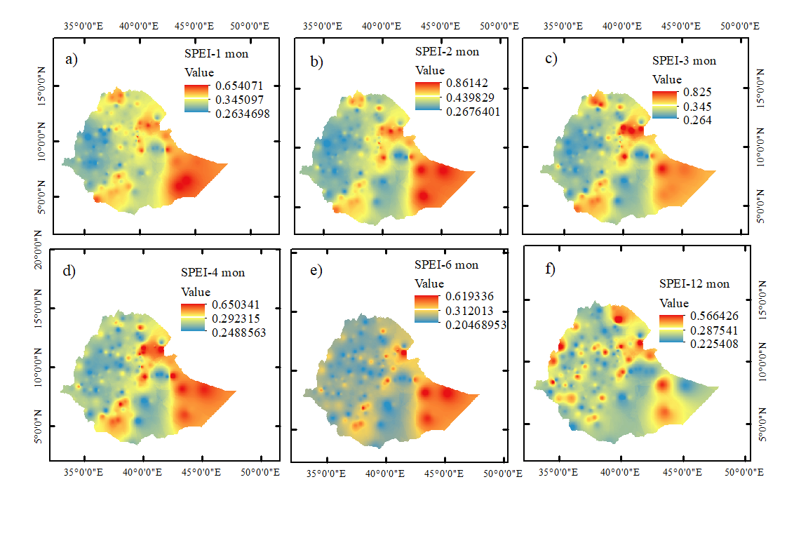
As indicated below Figure 2 and Figure 3, there was a positive correlation between soil moisture drought (SSMI-1 month) and meteorological drought of SPI and SPEI at different time scale. From the Figure 2, each panel (a-f) shows the Pearson correlation coefficient between soil moisture and SPI at different accumulation time scales. The color scale indicates the strength and direction of the correlation, and red-orange areas show high positive correlation, i.e., soil moisture strongly follows SPI fluctuations. Whereas yellow-green areas moderate correlation and blue-cyan areas indicating weak or even negative correlation (Figure 2a-f). Spatial propagation indicated that strong correlations (0.4-0.57) between SPI-1mon, SPI-2mon and SPI-3 month and SSMI-1mon over much of the western and central parts of Ethiopia, where soil moisture responds quickly to short-term rainfall anomalies (Figure 2a-c). Eastern low-lands and southeast showed weaker correlation, possibly because soils dry quickly, and short-term rainfall has less influence. As indicated by intermediated time scales (SPI-4mon to SPI-6mon), a slight decrease in correlation magnitude compared to short-term rainfall fluctuations in some western areas, but the correlation remains high in central highlands. Over drier lowland areas, the correlation indicated slightly increases with longer accumulation time, that implies soil moisture integrates rainfall anomalies over multiple months (Figure 2d-e). On the other hand, long time scale drought showed generally lower correlations in the range of 0.24-0.3 compared to shorter rime scale, which suggests at annual accumulation, other factors like evapotranspiration, ground water flow, land use dilute the direction between rainfall and near-surface soil moisture. While some pocket areas in the northwest still remain moderate correlations, indicating persistent hydrological remark (Figure 2f). In general, drought signal in soil moisture is most directly captured by short-term SPI in wetter, agriculturally important highlands. Over arid and semi-arid areas, longer term SPI better aligns with soil moisture anomalies, because these regions require sustained rainfall deficits to significantly impact soil moisture. Overall, the spatial drought pattern with respect to SPI at different time scale showed that drought development from meteorological to agricultural drought is not uniform, it propagates faster in humid zones but lags in dry zones due to storage effects.
The – depicts a summary diagram indicating how the correlation pattern changes from SPI-1mon to SPI-12mon and what that implies for drought monitoring lead time across Ethiopia.
The above figure shows spatial correlation between meteorological drought, that is measured by SPEI at different time scales, 1-12 months and soil moisture at 1-month time scale and describes sub-plots and time lags over Ethiopia. Each map (Figure 2a-f and Figure 3a-f) used 3 color bands showing correlation strength, red and orange show high correlation that means strong relationship between meteorological drought and soil moisture, yellow and green show moderate correlation while blue indicate low correlation. Accordingly, SPEI-1 month (Figure 3a) indicated moderate to high in many parts of central and southern Ethiopia, reflecting quick soil moisture response to short-term precipitation deficits. On the other hand, SPEI-2 month indicated strong and more widespread, particularly in southern and southeastern Ethiopia, indicating better soil moisture predictability at a slightly shorter time scale, because the correlation coefficient is greater than other time scales. Moreover, it suggests 2-month accumulation is a critical timescale for soil moisture dynamics in many parts of Ethiopia (Figure 3b). SPEI-3 month showed highest correlations observed in the northern, northeastern and eastern parts of Ethiopia. The higher time scale, the correlation coefficient declines over many areas, suggesting that soil moisture responds less to long-term SPEI at this scale in many areas.
3.2. Drought Intensity Propagation
Figure 4a-d show the distribution characteristics of the propagation of intensity of meteorological to soil drought that characterizes the influence of meteorological drought intensity on soil drought intensity. Accordingly, the average DIP was 0.959 for DIP 2-month, 0.8917 for DIP 3-month, 0.8953 for DIP 4-month and 0.82441 for DIP 6-month time scale, respectively. There is a peer-to-peer propagation from meteorological drought to soil drought, however, the peer-to-peer propagation is not uniform, various from place to place, time scale to time scale. DIP gradually changed from strong propagation from south and eastern part while weak propagation northern, norther western, central and western part of a country at 2-month time scale (Figure 4a). The 3-month time scale DIP indicated peer-to-peer propagation to strong propagation over Somali region, Afar, parts of southern Ethiopia, in general, the eastern south-eastern and north eastern part of the country indicated strong propagation with DIP is greater than 0.891 (Figure 4b).
3.3. Cereal Crop Yield Prediction
3.3.1. Model Evaluation
Different metrics can be used to assess machine learning algorithms, but this research focuses on two popular statistical measures: RMSE (root mean square error) and R2 (Coefficient of Determination). From Table 3, it is clear that the XGB regression model beats the RF regression model in terms of accuracy (64% to 74% vs. 54% to 72%), with the exception of Teff, where RF outperforms XGB. According to the algorithm, RF regression prediction outperforms the XGB model, but both RF and XGB equally predicted for Teff yield, averaging 2. 45 qt ha-1 of land (Table 3), with an RMSE of 2. 99 qt ha-1 to 5. 99 qt ha-1 for RF and 7. 81 qt ha-1 to 14. 47 qt ha-1 for XGB, respectively.
Figure 5 presents correlation heatmap, that visualizes how pairs of climatic variables and cereal crop yield are related. The color values indicate that red shaded color show positive correlation (values close to +1, meaning strong positive relationship), blue shaded color value indicates negative correlation (values close to -1, meaning strong negative relationship and near white or pale colors close to 0 show weak or no any correlation (Figure 5). To evaluate the connection between climatic factors and crop yields, multi-collinearity analysis was performed. The result indicated that strong correlation, exceeding 0.8, respectively (Figure 5). As a result, only variables with correlation coefficients greater than 0.8 or 0.9 were taken into consideration for deletion, and which variables were excluded from the machine learning process. This strategy was chosen because it was understood that variables that are highly correlated suggest similar information is being captured, making it more difficult to determine how each variable affects the dependent variable, and improve the reliability and usability of the models by giving priority to variables with lesser correlations. In such cases, and in feature importance analysis, this study selected only one of these variables as it could be sufficient, reducing the dimensionality of the dataset and improving model performance.
3.3.2. Feature Importance
The feature importance scores produced machine learning models using environmental variables as predictors for four cereal crops, Maize, Sorghum, Teff, and Wheat, are shown in Figure 6a-d. The variables are Tmax (maximum temperature), Tmin (minimum temperature), Prcp (precipitation), SM (soil moisture), and SPEI (standardized precipitation-evaporation index) representing drought/wetness, as well as SPEI1mon (1-month scale), SPEI2mon (2-month scale), and SPEI3mon (3-month scale). The model visually shows how much each characteristic adds to the model's predictions capability, Tmax and SPEI-3mon time scales being the most important predictors as indicated in Figure 6. Since a higher score indicates that the model depends more on that variable for generating precise forecasts.
According to the result, and as a result of preliminary summary, for example, Maize, Tmax and SPEI-3mon predominate indicating that Maize production is extremely susceptible to high temperatures and medium-term drought. It’s possible that the impact of rainfall is minimal since Tmax and SPEI have already taken into account the effects of water availability (Figure 6a). Tmax is the second most important driver of Sorghum next to SPEI-3mon as indicated by Figure 6b. Additionally, like Maize, Teff and Wheat seemed more impacted by drought stress and temperature fluctuations than by the actual quantity of rainfall. Rainfall, Tmin and SM have less of an impact (Figure 6c-d). The overall pattern showed that Tmax and SPEI-3mon were the most consistently important predictors. This suggests that excessive temperatures and dry conditions were better predictors of cereal crop yields than simply short-term rainfall. Integrated drought indices (SPEI), as opposed to simple rainfall, were more effective at describing water availability and agricultural stress due to low relevance of rainfall.
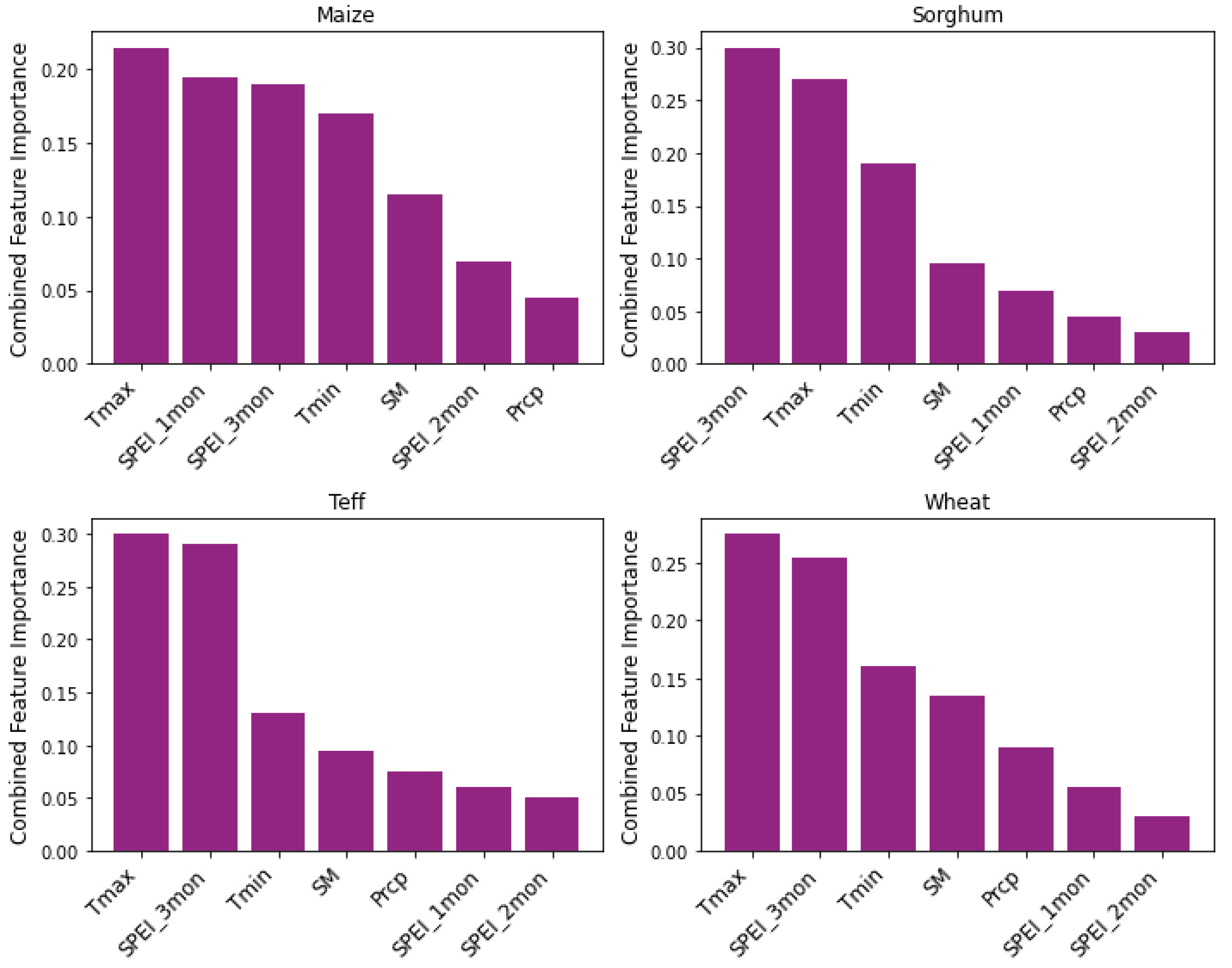
Figure 8 presents the combined feature importance from RF and XGB models, which normalizes each model's importance scores since they are visually comparable between crops. Furthermore, it combines the feature importance values by averaging them and generates four subplots for Maize, Sorghum, Teff, and Wheat, each with ranked purple bars. According to the findings, the most important environmental factors were the maximum temperature and drought indices dryness/wetness. For instance, Tmax and SPEI-3mon are key features that show how vulnerable cereal crop yield output is to high temperatures and medium-term drought (Figure 8). This demonstrates that combined feature importance plots take the strength of both RF and XGB regression results, giving a unified ranking of variables affecting cereal crop yields. In conclusion, maximum temperature and medium-term drought are consistently dominated across all cereals, i.e., heat stress and drought are the most influential factors.
Figure 7.
Feature importance score for XGBoost regressions.
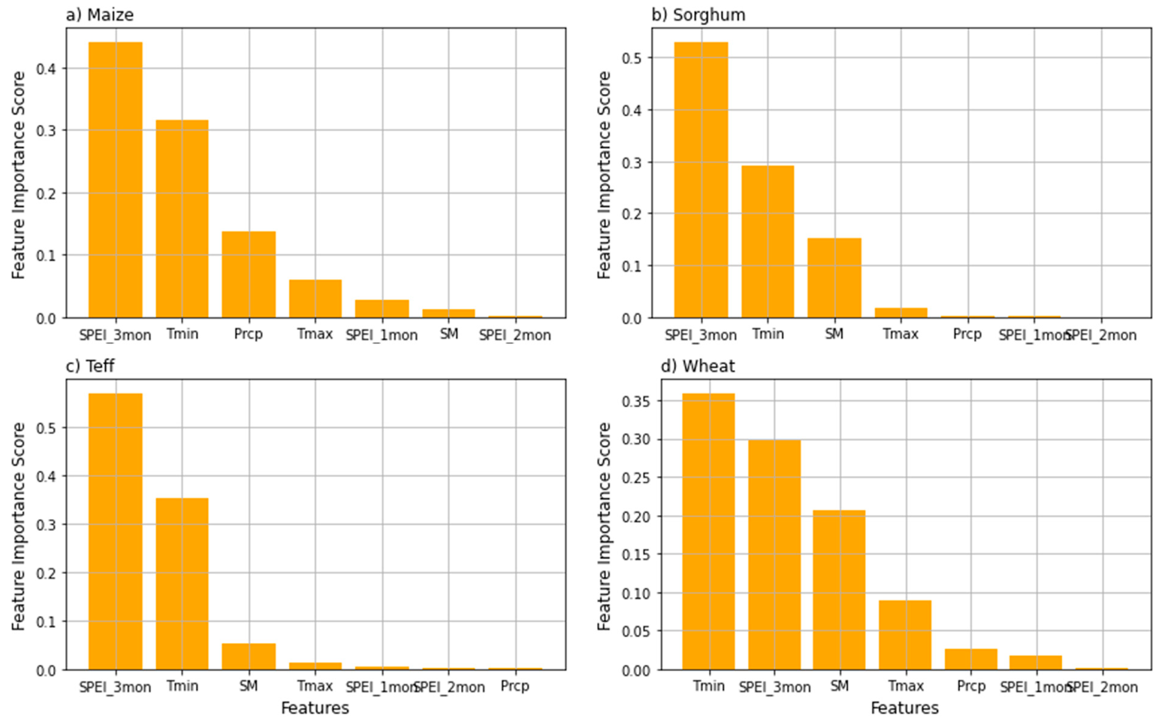
Figure 8.
Depicts feature importance score generated by ensemble of RF and XGBoost models.
4. Discussion and Conclusion
Discussion
Meteorological drought has the capability of activating other drought types and the most important factor causing soil moisture loss and soil drought, leading to crop failure [44]. Studies by other scholars indicated that local soil moisture deficits have also been shown to promote rainfall deficits, particularly in transitional regimes between humid and arid climate [66]. There are a number of spatial drought intensity pattern drivers, topography, soil types that sandy soils experience rapid intensification while clay soils showed delayed response [27]. On the other land vegetation reduces propagation through evapotranspiration buffering [61]. The other important factor is climate zone, that means arid and semi-arid areas propagates drought faster and more intense than humid zones [40]. The relationship between soil moisture and evapotranspiration is a key physical process between the land-atmosphere interface and breakthrough in the study of land-atmosphere interaction [67].
In this study, the correlation between soil drought and meteorological drought is generally positive and significant, but it varies depending on soil type, vegetation cover, topography, and climatic conditions (Figure 2 and Figure 3). Meteorological drought could have an impact on soil moisture and then leading to agricultural drought resulting in crop production. Drought monitoring results based on agricultural drought index have a certain lag compared with meteorological drought. The method to determine the response lag time is to calculate the correlation coefficient between SSMI and SPEI of each time scale, and select the time scale with the greatest correlation coefficient. The response delay characteristics of agricultural drought to meteorological drought in different months were quantitatively discussed according to the calculation results. The correlation coefficients between monthly scale SSMI and SPEI of different time scales were shown Figure 2 and Figure 3.
The variables affecting crop yield can be categorized as primary or secondary. Temperature, precipitation, insolation, soil pH, soil moisture, soil nutrient content, and agronomic factors such as planting dates are examples of key environmental indicators [68]. The main focus of this research was on key elements that have a major impact on crop growth and development, as well as on variables frequently employed in yield forecasting [69]. The independent variables most frequently used in machine learning models are drought indices, rainfall soil moisture, minimum temperature, and maximum temperature. According to research finding, temperature has variable effects on cereal output yield prediction [70]. The finding of this study indicated that maximum temperature and SPEI at medium time scale were the most feature important, strongly influential, this might be extreme heat during flowing stage reduce crop yields. Maximum temperature often varies significantly across time and space, offering more predictive signal than features that are relatively constant, often drive stress responses in plants. Moreover, maximum temperature might interact with other features, i.e., rainfall, to produce complex effects. According to a combined feature importance result as depicted in Figure 8, and through the lens of climate change impacts on cereal crop yields, the relationship is becomes quite clear. Accordingly, top predictors are maximum temperature, short and medium term drought conditions are all climate-sensitive variables that directly respond to long-term warming, heat waves, and altered rainfall patterns. Climate change amplifies both temperature extremes and hydrological variability, meaning the most important features indicating climate change would shift most.
5. Conclusions
Drought intensity in Ethiopia shows spatially heterogeneous propagation, often initiating in the east/southeast and spreading westward with varying intensity depending on local climatic and environmental conditions. The 2- to 4-month SPEI timescales are most critical in capturing and mapping this propagation. In general, drought intensity in Ethiopia showed spatially heterogeneous propagation, often indicating in the east and south-east, then spreading westward with varying intensity depending on local climatic and environmental conditions. The 2-to 3-month SPEI time scales are most critical in capturing and mapping this propagation.
The study recommends the following adaptation strategies based on feature importance, breeding for heat tolerance in maize and wheat, water saving agronomy and supplemental irrigation for all crops where feasible. Shifting planting date to avoid peak heat period, diversifying cropping systems to spread climate risks.
Supplementary Material
The following supporting information can be downloaded at the website of this paper posted on Preprints.org.
Ethics Statement
Informed consent is not applicable
Funding
This research received no fund
Author Contribution
Tadele Badebo Badacho has solely carried out this research work.
Data Availability Statement
The data used for this research is freely available on reasonable request of the author
Acknowledgments
The author would like to thank the Ethiopian Meteorology Institute for freely providing climate data, Ethiopian Meteorological Society and its staff financial supporting for data collecting.
Conflict of Interest
The author declares no conflict of interest
References
- Y. Zhou, J. Y. Zhou, J. Li, W. Jia, F. Zhang, H. Zhang, and S. Wang, “The Evolution of Drought and Propagation Patterns from Meteorological Drought to Agricultural Drought in the Pearl River Basin,” 2025.
- C. Springs, N. C. Springs, N. Carolina, O. Board, M. Regional, and N. Drought, “THE DROUGHT MONITOR,” no. April, 2002.
- M. Neelam and C. Hain, “Global Flash Droughts Characteristics : Onset, Duration, and Extent at Watershed Scales,” 2024. [CrossRef]
- M. Temesgen, “Determinants of Tillage Frequency Among Smallholder Farmers in Two Semi- Arid Areas in Ethiopia Determinants of tillage frequency among smallholder farmers in two semi-arid areas in Ethiopia,” no. December, 2008. [CrossRef]
- T. Zolt, “The patterns of potential evapotranspiration and seasonal aridity under the change in climate in the upper Blue Nile basin, Ethiopia,” vol. 641, no. 22, 2024. 20 October. [CrossRef]
- S. Liu et al., “Spatiotemporal response of agricultural drought to meteorological drought in the upper Hanjiang River Basin from three-dimensional perspective,” Agric. For. Meteorol., vol. 368, p. 110531, 2025.
- T. H. E. Need and F. O. R. Proactive, “Global Drought Snapshot,” 2023.
- A. Dai, “Drought under global warming :a review,” pp. 45–65, 2011. [CrossRef]
- W. Zhang et al., “Dynamic Characteristics of Meteorological Drought and Its Impact on Vegetation in an Arid and Semi-Arid Region,” 2023.
- J. K. Green, H. J. K. Green, H. Alemohammad, J. A. Berry, and P. Gentine, “Regionally strong feedbacks between the atmosphere and terrestrial biosphere,” no. June, 2017. [CrossRef]
- W. M. O. WMO, “Drought monitoring and early warning : concepts, progress and future challenges,” World Meteorogical Organ., no. 1006, p. 24, 2006, [Online]. Available: http://www.wamis.org/agm/pubs/brochures/WMO1006e.
- Y. Liu, F. Y. Liu, F. Shan, H. Yue, X. Wang, and Y. Fan, “Global analysis of the correlation and propagation among meteorological, agricultural, surface water, and groundwater droughts,” J. Environ. Manage., vol. 333, p. 117460, 2023.
- M. Dai et al., “Propagation characteristics and mechanism from meteorological to agricultural drought in various seasons,” J. Hydrol., vol. 610, p. 127897, 2022.
- B. N. Wolteji, S. T. B. N. Wolteji, S. T. Bedhadha, S. L. Gebre, E. Alemayehu, and D. O. Gemeda, “Multiple indices based agricultural drought assessment in the rift valley region of Ethiopia,” Environ. Challenges, vol. 7, p. 100488, 2022.
- J. Wu, X. J. Wu, X. Chen, H. Yao, and D. Zhang, “Multi-timescale assessment of propagation thresholds from meteorological to hydrological drought,” Sci. Total Environ., vol. 765, p. 144232, 2021.
- A. K. Mishra and V. P. Singh, “Review paper A review of drought concepts,” J. Hydrol., vol. 391, no. 1–2, pp. 202–216, 2010. [CrossRef]
- W. J. Quirk and U. States, “Drought in the Sahara : A Biogeophysical Feedback Mechanism,” no. 75, 2014. 19 March. [CrossRef]
- S. Huang, P. S. Huang, P. Li, Q. Huang, G. Leng, B. Hou, and L. Ma, “The propagation from meteorological to hydrological drought and its potential influence factors,” J. Hydrol., vol. 547, pp. 184–195, 2017.
- A. I. Gevaert, T. I. E. A. I. Gevaert, T. I. E. Veldkamp, and P. J. Ward, “The effect of climate type on timescales of drought propagation in an ensemble of global hydrological models,” pp. 4649–4665, 2018.
- J. Wei et al., “Drought variability and its connection with large-scale atmospheric circulations in Haihe River Basin,” Water Sci. Eng., 2020. [CrossRef]
- K. K. Kumar, B. K. K. Kumar, B. Rajagopalan, and M. A. Cane, “On the Weakening Relationship Between the Indian Monsoon and ENSO Published by : American Association for the Advancement of Science Stable URL : https://www.jstor.org/stable/2898422 Linked references are available on JSTOR for this article : You may need to log in to JSTOR to access the linked references. On the Weakening Relationship Between the Indian Monsoon and ENSO,” vol. 284, no. 5423, pp. 2156–2159, 1999.
- E. Viste, D. E. Viste, D. Korecha, and A. Sorteberg, “Recent drought and precipitation tendencies in Ethiopia,” Theor. Appl. Climatol., vol. 112, no. 3–4, 2013. [CrossRef]
- G. M. Tullu, “Impact of ENSO on Drought in Borena Zone, Ethiopia,” no. January, 2025. [CrossRef]
- J. M. Warner and M. L. Mann, “Agricultural Impacts of the 2015 / 2016 Drought in Ethiopia Using High- Agricultural Impacts of the 2015 / 2016 Drought in Ethiopia Using High-Resolution Data Fusion Methodologies,” no. October, 2018. [CrossRef]
- D. Korecha and A. G. Barnston, “Predictability of June-September rainfall in Ethiopia,” Mon. Weather Rev., vol. 135, no. 2, pp. 628–650, 2007. [CrossRef]
- D. Korecha and A. Sorteberg, “Validation of operational seasonal rainfall forecast in Ethiopia,” Water Resour. Res., vol. 49, no. 11, pp. 7681–7697, 2013. [CrossRef]
- A. Review, “Research Progress and Conceptual Insights on Drought Impacts and Responses among Smallholder Farmers in South Africa :,” 2022.
- F. Mare, Y. T. F. Mare, Y. T. Bahta, and W. Van Niekerk, “Development in Practice The impact of drought on commercial livestock farmers in South Africa,” vol. 4524, 2018. [CrossRef]
- W. 1267. 2019.
- E. for the C. of H. A. OCHA, “DROUGHT RESPONSE of ETHIOPIA,” vol. 2022, no. December, 2022, [Online]. Available: https://reliefweb. 2022.
- B. K. Wossenyeleh, V. U. B. K. Wossenyeleh, V. U. Brussel, and A. S. Kasa, “Drought propagation in the hydrological cycle in a semiarid region : a case study in the Bilate catchment, Ethiopia Drought propagation in the hydrological cycle in a semiarid region : a case study in the Bilate catchment, Ethiopia,” no. February, 2022. [CrossRef]
- G. M. Tullu and M. T. Guta, “Effects of meteorological and agricultural droughts on crop production in Arsi Effects of meteorological and agricultural droughts on crop production in Arsi Zone Ethiopia,” no. January, 2025. [CrossRef]
- F. Wang et al., “Dynamic variation of meteorological drought and its relationships with agricultural drought across China,” Agric. Water Manag., vol. 261, p. 107301, 2022.
- Y. Dahhane, V. Y. Dahhane, V. Ongoma, A. Hadri, M. H. Kharrou, and O. Hakam, “Probabilistic linkages of propagation from meteorological to agricultural drought in the North African semi-arid region,” 2023.
- S. Park, J. S. Park, J. Lee, M. Jeong, S. Park, Y. Kim, and H. Yoon, “Identification of propagation characteristics from meteorological drought to hydrological drought using daily drought indices and lagged correlations analysis Journal of Hydrology : Regional Studies Identification of propagation characteristics from meteorological drought to hydrological drought using daily drought indices and lagged correlations analysis,” J. Hydrol. Reg. Stud., vol. 55, no. November, p. 101939, 2024. [CrossRef]
- C. Von Matt, R. C. Von Matt, R. Muelchi, L. Gudmundsson, and O. Martius, “Compound droughts under climate change in Switzerland,” vol. 2022, no. January, pp. 1–37, 2024.
- D. Muthuvel and X. Qin, “Probabilistic Analysis of Future Drought Propagation, Persistence, and Spatial Concurrence in Monsoon-Dominant Asian Region under Climate Change,” no. March, 2025.
- M. Rashid, B. S. M. Rashid, B. S. Bari, Y. Yusup, M. A. Kamaruddin, and N. Khan, “A Comprehensive Review of Crop Yield Prediction Using Machine Learning Approaches With Special Emphasis on Palm Oil Yield Prediction,” vol. 9, 2021. [CrossRef]
- P. Capuano, M. P. Capuano, M. Sellerino, A. Ruocco, W. Kombe, and K. Yeshitela, “Climate change induced heat wave hazard in eastern Africa: Dar Es Salaam (Tanzania) and Addis Ababa (Ethiopia) case study,” p. 3366, Apr. 2013.
- R. J. Zomer, X. R. J. Zomer, X. Jianchu, and A. Tr, “Version 3 of the Global Aridity Index and Potential Evapotranspiration Database,” pp. 1–15, 2022. [CrossRef]
- M. Gaillard, N. M. Gaillard, N. Whitehouse, M. Madella, K. Morrison, and L. Von Gunten, “Past land-use and land-cover change:the challenge of quantification at the subcontinental to global scales,” vol. 26, no. 1, 2018.
- T. Dinku and S. J. Connor, “Improving availability, access and use of climate information,” no. December, 2014.
- T. Dinku, R. T. Dinku, R. Faniriantsoa, R. Cousin, I. Khomyakov, and A. Vadillo, “ENACTS : Advancing Climate Services Across Africa,” vol. 3, no. January, pp. 1–16, 2022. [CrossRef]
- Q. Li, A. Q. Li, A. Ye, Y. Zhang, and J. Zhou, “The Peer-To-Peer Type Propagation From Meteorological Drought to Soil Moisture Drought Occurs in Areas With Strong Land-Atmosphere Interaction Water Resources Research,” 2022. [CrossRef]
- A. G. & Karthikeyan, “Role of Initial Conditions and Meteorological Drought in Soil Moisture Drought Propagation: An Event-Based Causal Analysis Over South Asia,” pp. 1–21, 2024. [CrossRef]
- R. J. Zomer and A. Trabucco, “Global Aridity Index and Potential Evapo-Transpiration ( ET 0 ) Database v3 Methodology and Dataset Description,” no. March, pp. 1–6, 2022.
- E. Elias, P. F. E. Elias, P. F. Okoth, J. J. Stoorvogel, and G. Berecha, “Cereal yields in Ethiopia relate to soil properties and N and P fertilizers,” Nutr. Cycl. Agroecosystems, vol. 126, no. 2, pp. 279–292, 2023. [CrossRef]
- CSA, “The Federal Democratic Republic of Ethiopia Central Statistical Agency (CSA) Report on Area, Production and Farm Management Practice of Belg Season Crops for Private Peasant Holdings,” vol. V, p. 25, 2021.
- E. October. 2019.
- CSA, “The Federa Democratic Republic of Ethiopia, the Centeral Statistical Agency (CSA) Report on Area and Production of Majr Crops,” vol. I, 2020.
- L. Cochrane and Y. W. Bekele, “Data in Brief Average crop yield ( 2001 – 2017 ) in Ethiopia : Trends at national, regional and zonal levels,” Data Br., vol. 16, pp. 1025–1033, 2018. [CrossRef]
- S. M. Vicente-Serrano, S. S. M. Vicente-Serrano, S. Beguería, and J. I. López-Moreno, “A multiscalar drought index sensitive to global warming: the standardized precipitation evapotranspiration index,” J. Clim., vol. 23, no. 7, pp. 1696–1718, 2010.
- Z. You et al., “Mechanisms of meteorological drought propagation to agricultural drought in China : insights from causality chain,” npj Nat. Hazards, 2025. [CrossRef]
- G. H. Hargreaves and R. G. Allen, “History and Evaluation of Hargreaves Evapotranspiration Equation,” J. Irrig. Drain. Eng., vol. 129, no. 1, pp. 53–63, 2003. [CrossRef]
- P. Pandya and N. K. Gontia, “Early crop yield prediction for agricultural drought monitoring using drought indices, remote sensing, and machine learning techniques,” no. January, 2024. [CrossRef]
- H. Shi, “A New Perspective on Drought Propagation : Causality Geophysical Research Letters,” pp. 1–9, 2022. [CrossRef]
- T. Dinku, “The Climate Data Tool : Enhancing Climate Services Across Africa,” no. April, 2022. [CrossRef]
- K. K. T. G, C. K. K. T. G, C. Shubha, and S. A. Sushma, “Random Forest Algorithm for Soil Fertility Prediction and Grading Using Machine Learning,” no. 1, pp. 1301–1304, 2019. [CrossRef]
- R. Genuer et al., “Variable selection using Random Forests To cite this version : HAL Id : hal-00755489,” vol. 31, no. 14, 2012.
- D. Wallach, D. D. Wallach, D. Makowski, and J. W. Jones, “Working with Dynamic Crop Models, 2nd Edition Table of Contents,” no. December, pp. 1–2, 2013.
- S. Kim et al., “Modeling Temperature Responses of Leaf Growth, Development, and Biomass in Maize with MAIZSIM,” pp. 1523–1537, 2012. [CrossRef]
- T. Chai, R. R. T. Chai, R. R. Draxler, and C. Prediction, “Root mean square error ( RMSE ) or mean absolute error ( MAE )? – Arguments against avoiding RMSE in the literature,” no. 2005, pp. 1247–1250, 2014. [CrossRef]
- P. Krause and D. P. Boyle, “Advances in Geosciences Comparison of different efficiency criteria for hydrological model assessment,” pp. 89–97, 2005.
- J. H. Jeong, J. P. J. H. Jeong, J. P. Resop, N. D. Mueller, and D. H. Fleisher, “Random Forests for Global and Regional Crop Yield Predictions,” pp. 1–15, 2016. [CrossRef]
- B. Toleva, “The Proportion for Splitting Data into Training and Test Set for the Bootstrap in Classification Problems,” no. May, 2021. [CrossRef]
- H. Xu, X. H. Xu, X. Wang, C. Zhao, S. Shan, and J. Guo, “Seasonal and aridity influences on the relationships between drought indices and hydrological variables over China,” Weather Clim. Extrem., vol. 34, p. 100393, 2021. [CrossRef]
- J. Gaona, P. J. Gaona, P. Quintana-seguí, M. J. Escorihuela, A. Boone, and M. C. Llasat, “Interactions between precipitation, evapotranspiration and soil-moisture-based indices to characterize drought with high-resolution remote sensing and land-surface model data,” pp. 3461–3485, 2022.
- S. Data, “Selection of Independent Variables for Crop Yield Prediction Sensing Data,” 2021.
- O. M. Adisa et al., “Application of Artificial Neural Network for Predicting Maize Production in South Africa,” pp. 1–17. [CrossRef]
- S. Kim and H. Kim, “A new metric of absolute percentage error for intermittent demand forecasts,” Int. J. Forecast., vol. 32, no. 3, pp. 669–679, 2016. [CrossRef]
Figure 1.
Shows a) Digital elevation map (DEM) in meter, b) Mean Annual Precipitation (MAP) in mm and c) Aridity Index map.
Figure 1.
Shows a) Digital elevation map (DEM) in meter, b) Mean Annual Precipitation (MAP) in mm and c) Aridity Index map.
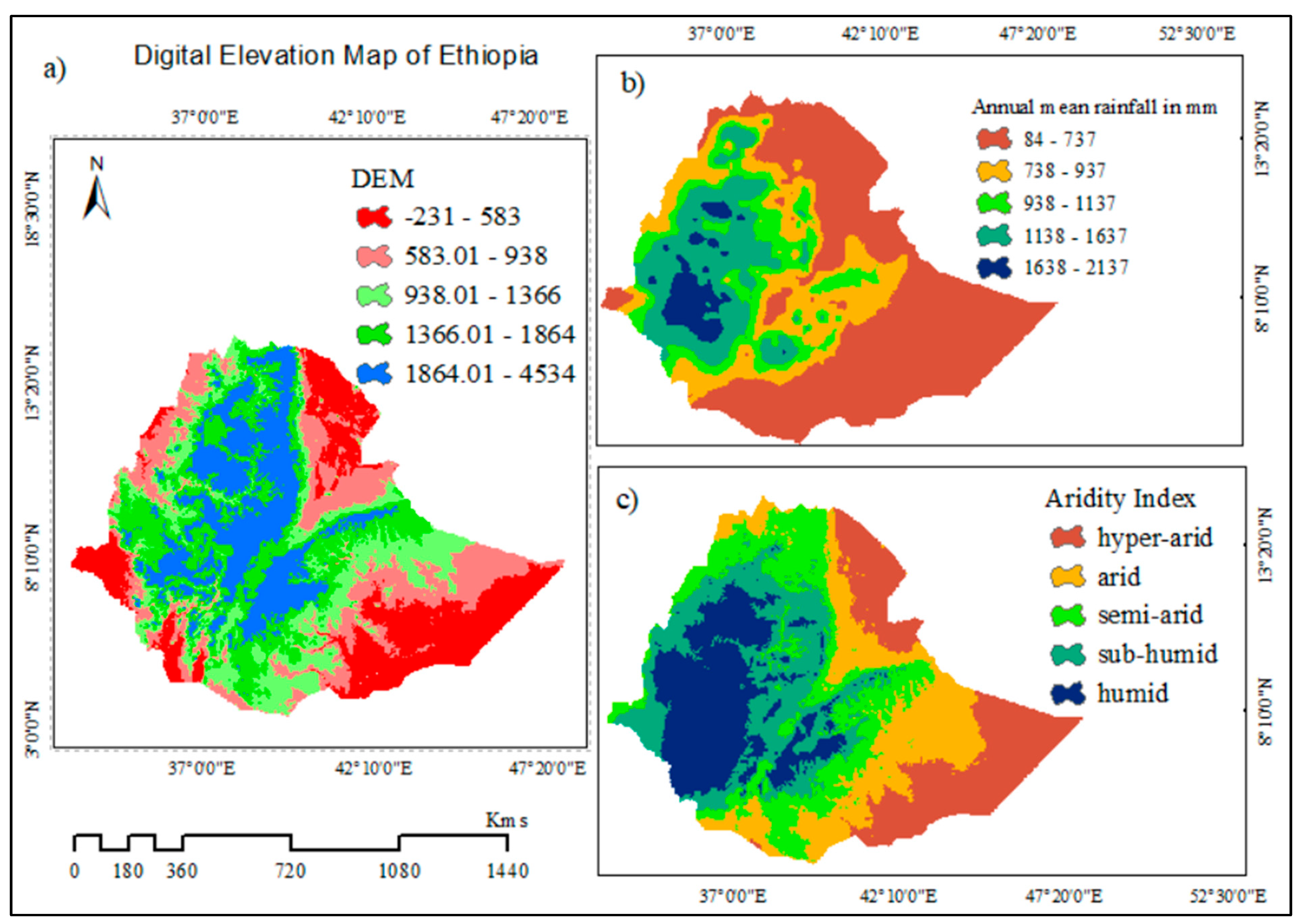
Figure 2.
Pearson Correlation Coefficient between Soil Moisture Drought and SPI at (a) 1-month, (b) 2-month, (c) 3-month, (d) 4-month, (e) 6-month and (f) 12-month time scale.
Figure 2.
Pearson Correlation Coefficient between Soil Moisture Drought and SPI at (a) 1-month, (b) 2-month, (c) 3-month, (d) 4-month, (e) 6-month and (f) 12-month time scale.
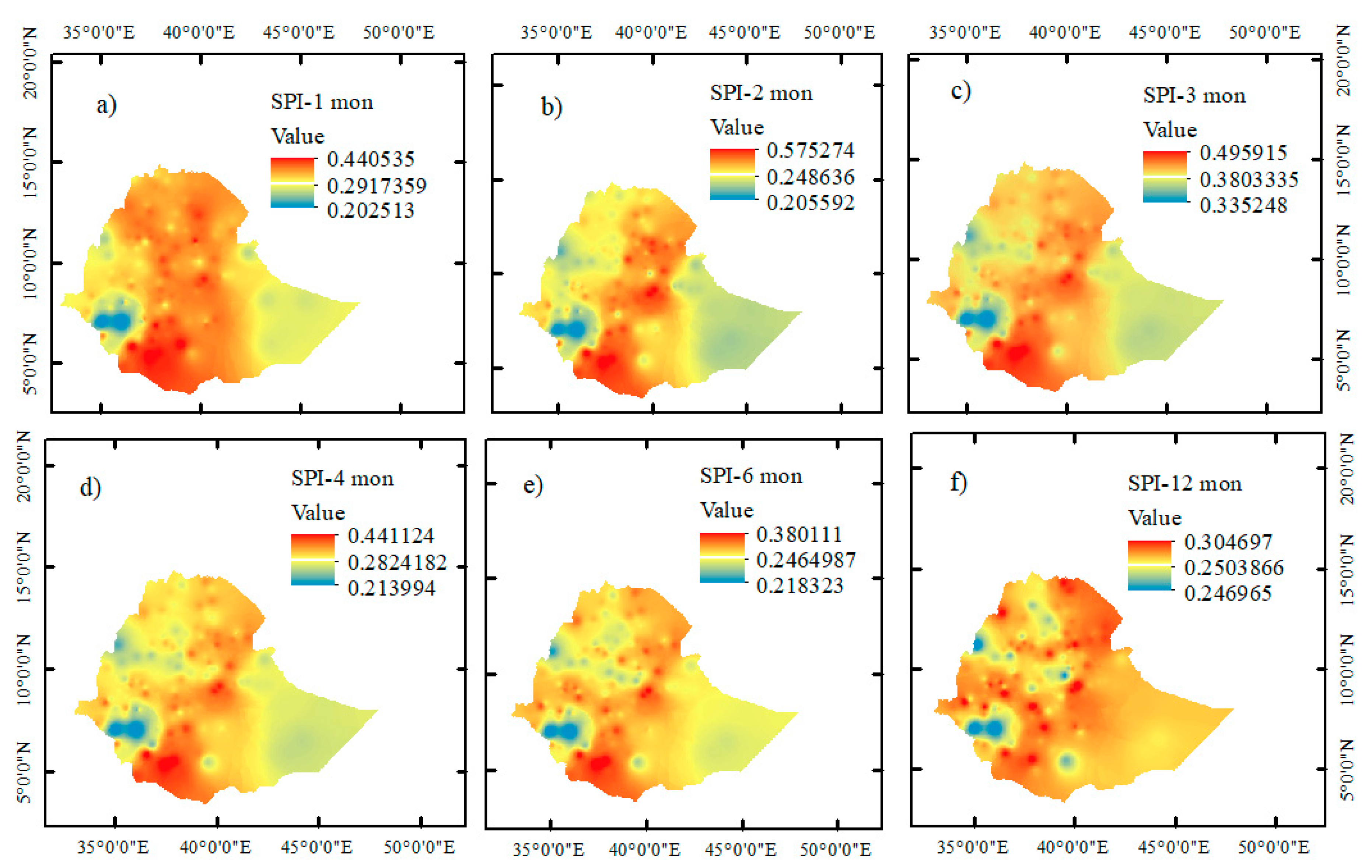
Figure 3.
Pearson Correlation Coefficient between Soil Moisture Drought and SPEI at (a) 1-month, (b) 2-month, (c) 3-month, (d) 4-month, (e) 6-month and (f) 12-month time scale.
Figure 3.
Pearson Correlation Coefficient between Soil Moisture Drought and SPEI at (a) 1-month, (b) 2-month, (c) 3-month, (d) 4-month, (e) 6-month and (f) 12-month time scale.
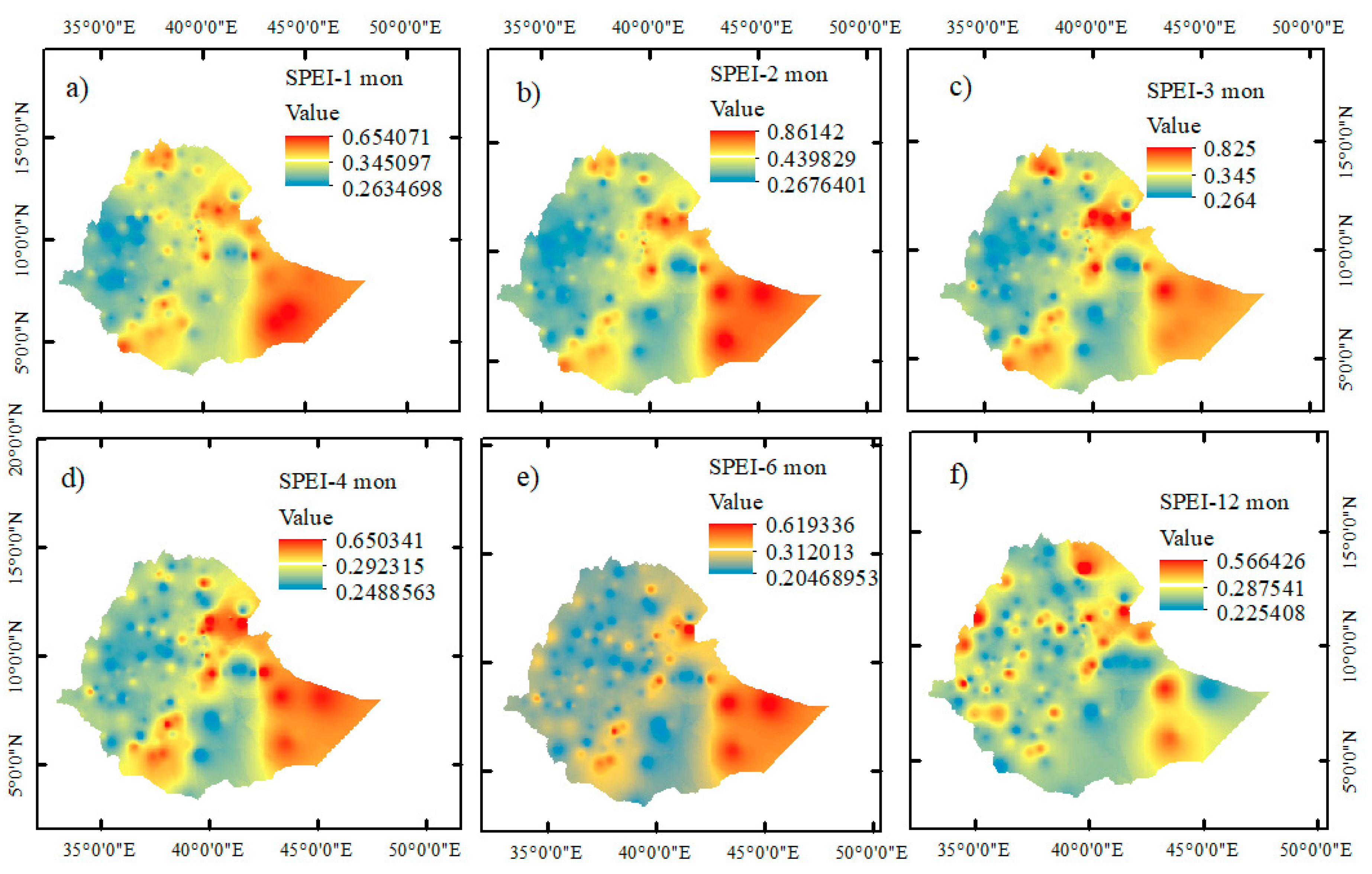
Figure 4.
Spatial characteristics of DIP.
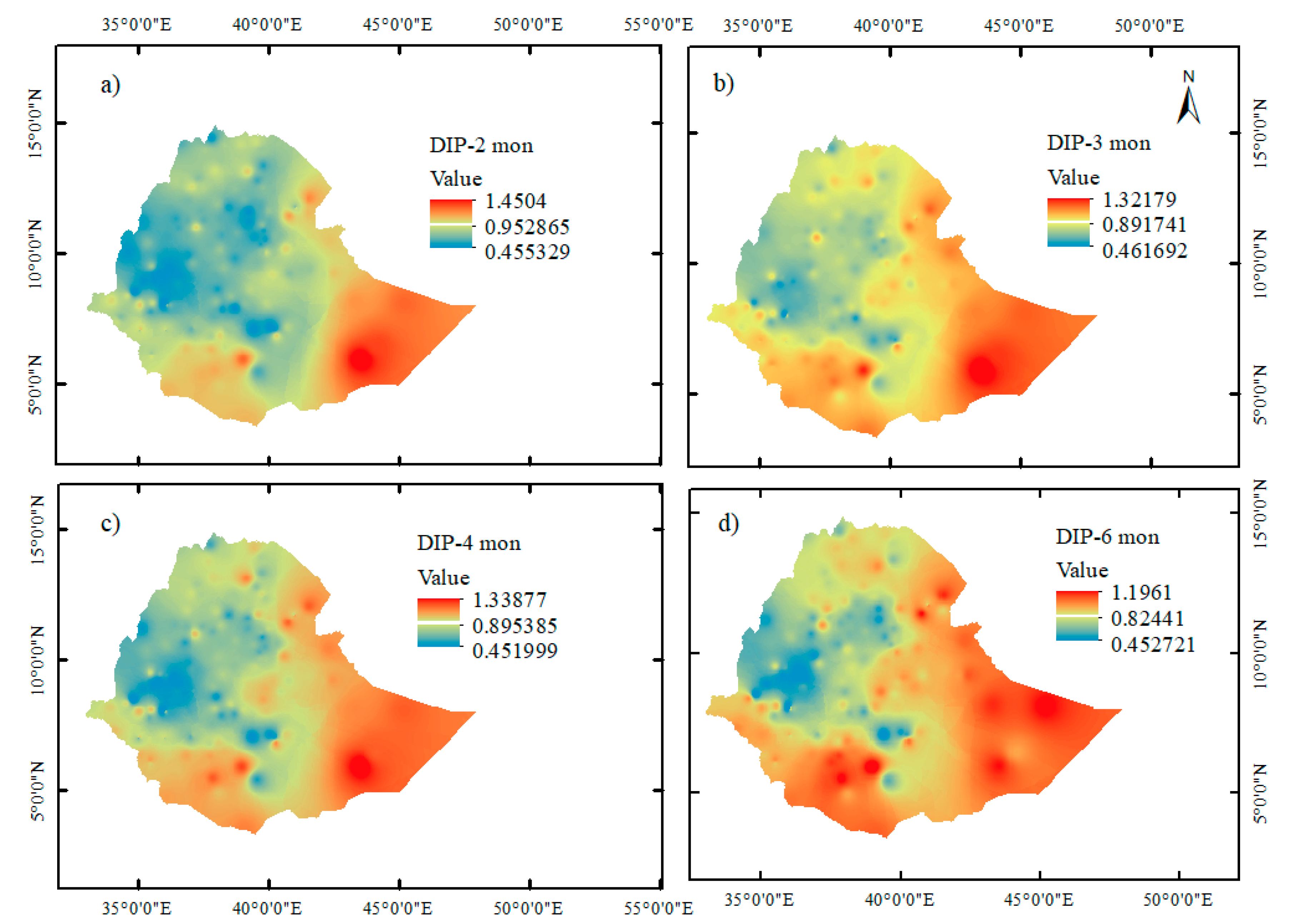
Figure 5.
Presents multi-collinearity analysis indicating the relationship between cereal crop yield and climatic variables. It shows the existence of high correlations between some variables that affect the model reliability and interpretability.
Figure 5.
Presents multi-collinearity analysis indicating the relationship between cereal crop yield and climatic variables. It shows the existence of high correlations between some variables that affect the model reliability and interpretability.
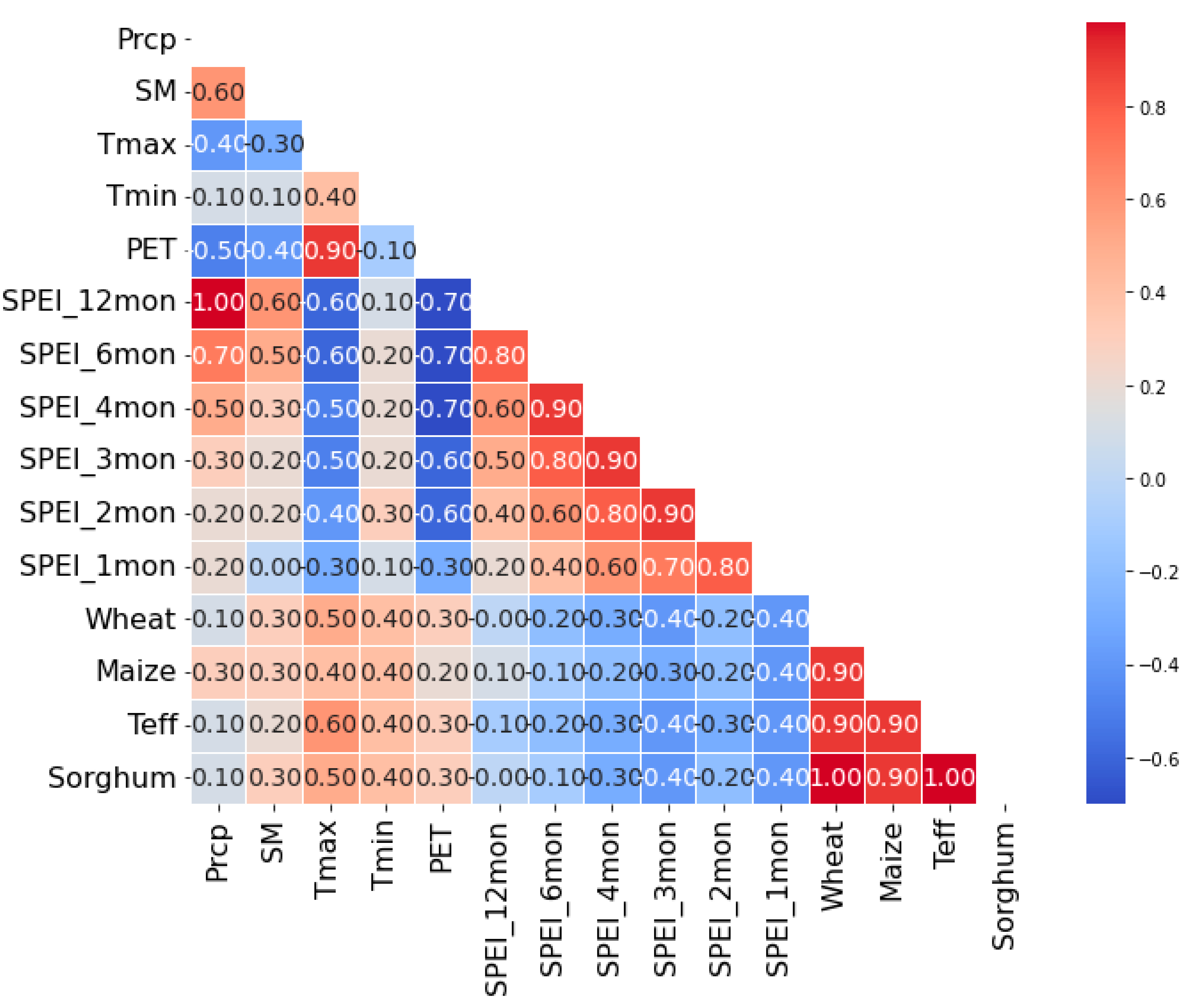
Figure 6.
Feature importance score for Random Forest regressions.
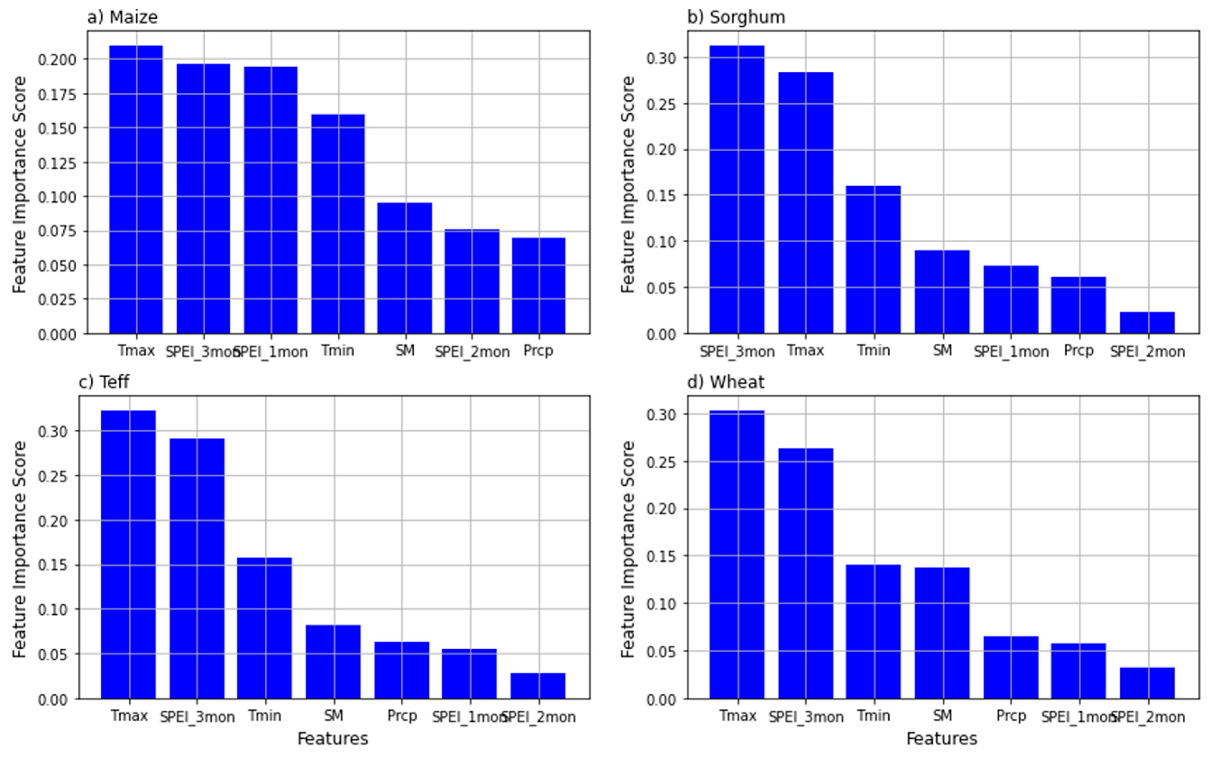

Table 1.
Classification standards of dryness and wetness based on the SPEI index.
| SPEI Values | Categories of Climatic Moisture | SPEI Values | Categories of Climatic Moisture |
|---|---|---|---|
| ≥ 2.00 | Extremely wet | -1.49 to -1.00 | Moderately dry |
| 1.05 to 1.99 | Severely wet | -1.99 to -1.50 | Severely dry |
| 1.00 to 1.49 | Moderately wet | ≤ -2 | Extremely dry |
Source: [52]. SSMI less than 0 indicates that the soil moisture is less than normal showing a state of soil water deficit. Conversely, an SSMI greater than 0 indicates that the soil moisture is greater than the normal value showing a state of soil moisture surplus and the value indicates the degree of deviation from the normal value.
Table 2.
Classification of Drought Propagation Index.
| DIP | Index Range | DIP | Index Range |
|---|---|---|---|
| (0.9, 1.1) | Peer-to-peer | ||
| (1.1, 1.2) | Mildly strong | (0.8, 0.9) | Middy weak |
| (1.2, 1.3) | Moderately strong | (0.7, 0.8) | Moderately weak |
| (1.3, +∞) | Extra strong | (0.0, 0.7) | Extra weak |
Table 3.
RF vs XGB performance by different cereal crops.
| Crop | RF MAE (qt/ha) | RF RMSE (qt/ha) | RF R² | XGB MAE (qt/ha) | XGB RMSE (qt/ha) | XGB R² |
|---|---|---|---|---|---|---|
| Wheat | 3.4046 | 4.04 | 0.59 | 2.9054 | 8.85 | 0.64 |
| Maize | 4.5439 | 5.98 | 0.54 | 2.7817 | 14.47 | 0.71 |
| Sorghum | 2.6566 | 2.99 | 0.72 | 1.9426 | 7.81 | 0.74 |
| Teff | 2.2363 | 2.45 | 0.56 | 2.7817 | 2.45 | 0.45 |
Disclaimer/Publisher’s Note: The statements, opinions and data contained in all publications are solely those of the individual author(s) and contributor(s) and not of MDPI and/or the editor(s). MDPI and/or the editor(s) disclaim responsibility for any injury to people or property resulting from any ideas, methods, instructions or products referred to in the content. |
© 2025 by the authors. Licensee MDPI, Basel, Switzerland. This article is an open access article distributed under the terms and conditions of the Creative Commons Attribution (CC BY) license (http://creativecommons.org/licenses/by/4.0/).
Copyright: This open access article is published under a Creative Commons CC BY 4.0 license, which permit the free download, distribution, and reuse, provided that the author and preprint are cited in any reuse.


