
Submitted:
10 September 2025
Posted:
11 September 2025
You are already at the latest version
Abstract
Accurate banana yield prediction is essential for optimizing agricultural management and ensuring food security in tropical regions, yet traditional estimation methods remain labor-intensive and error - prone. This study developed a predictive model for banana yield in Buena Fé, Ecuador, using Random Forest integrated with phenological data, soil properties, spectral technology, and UAV imagery. Data were collected from a 75.2 ha banana farm divided into 26 lots, combining multispectral drone imagery, soil physicochemical analyses, and banana agronomic measurements (height, diameter, bunch weight). A rigorous variable selection process identified six key predictors: NDVI, plant height, plant diameter, soil nitrogen, porosity, and slope. Three machine learning algorithms were compared through 5-fold cross-validation with systematic hyperparameter optimization. Random Forest demonstrated superior performance with R²=0.956 and RMSE=1164.9 kg ha⁻¹, representing only 2.79% of mean production. NDVI emerged as the most influential predictor (importance=0.212), followed by slope (0.184) and plant structural variables. Local sensitivity analysis revealed distinct response patterns between low and high production scenarios, with plant diameter showing greatest impact (+74.9 boxes ha-1) under limiting conditions, while NDVI dominated (-140.4 boxes ha-1) under optimal conditions. The model provides a robust tool for precision agriculture applications in tropical banana production systems.
Keywords:
banana
; UAV
; random forest
; ecuadorian littoral region
; soil properties
; yield
1. Introduction
Bananas (Musa AAA) are one of the most important crops worldwide, both for their nutritional value and economic impact, especially in tropical regions like Ecuador [1], which is one of the main global exporters [2]. However, banana production faces significant challenges, such as climate variability, soil degradation, and the need to optimize resources to maintain sustainability and competitiveness of the sector [3]. In this context, accurate crop yield prediction becomes an essential tool for informed decision-making in agricultural management.
Traditionally, in some Latin American regions, yield estimation has been based on empirical methods and manual observations, which are laborious, costly, and prone to errors [4,5]. Nevertheless, the advancement of technologies such as remote sensing, unmanned aerial vehicles (UAVs), and supervised machine learning has opened new possibilities to improve precision and efficiency in agricultural yield prediction [6,7,8]. These technologies allow capturing and analyzing high spatial and temporal resolution data, integrating key variables such as crop phenology, soil physicochemical properties, and spectral reflectance, which are directly related to plant growth and development [9].
Banana phenology, which includes critical stages such as flowering and fruit filling, is a fundamental indicator for predicting yield [10]. On the other hand, soil physicochemical parameters, such as pH, organic matter, and nutrient availability, directly influence crop productivity [11]. Spectral technology, through multispectral and hyperspectral sensors, allows monitoring plant health status and vigor through vegetation indices, such as NDVI (Normalized Difference Vegetation Index), which are correlated with biomass and productive potential [9]. Additionally, UAVs offer a versatile platform for capturing high-resolution images, facilitating spatial and temporal analysis of large crop extensions.
The use of Random Forest techniques, multiple linear regression, neural networks, allows integrating these heterogeneous and complex variables to generate robust predictive models [12,13]. These models not only improve precision in yield estimation, but also identify patterns and non-linear relationships between variables, resulting in a powerful tool for precision agriculture [14].
This article aims to develop a predictive model for banana yield in the central tropical region of Ecuador, using Random Forest (RF) and data obtained from productive phenology, soil physicochemical parameters, spectral technology, and UAVs. The expected results will contribute to optimizing crop management, improving productivity, and promoting more sustainable agricultural practices in one of the world’s most important banana regions.
2. Materials and Methods
2.1. Study Area
The work was conducted on a banana farm located in Buena Fe city (WGS84: long-0.818409; lat -79.479516), Los Ríos province, which is located in the central-north of Ecuador’s coastal region. Los Ríos province is Ecuador’s main banana yield province [15]. It has the following geophysical characteristics: altitude of 103 m.a.s.l., with a tropical rainy climate of 22.6°C and 2257.85 mm of precipitation on average [16]. The study farm has an area of 75.2 ha (Figure 1) and is divided into 26 administrative plots, plots that were divided in relation to vegetation conditions, which guarantees homogeneity for analysis.
2.2. Spectral Data and UAV Images
The acquisition of multispectral and RGB data was performed using a DJI Mavic 3M drone equipped with an integrated four-spectral-band system (Green: 560, Red: 650, Red Edge: 730, NIR: 860), and a wide-angle sensor with 4/3” CMOS sensor with 20 megapixels. The system operated at 80 m altitude, generating a spatial resolution of 6.4 cm/pixel for multispectral bands and 1.4 cm/pixel for RGB, following the relationship GSD = (height × pixel size) / focal distance [17]. Georeferencing employed a D-RTK 2 Mobile Station, achieving absolute precision of ±10 cm (horizontal) and ±18 cm (vertical).
Operational parameters and quality control: flights were executed between 10:00-14:00 (local time) under cloud conditions of 65% ± 5%, wind of 1.1 m/s and average irradiance of 750 ± 100 W/m2. Double grid routes were implemented with 80% frontal and lateral overlap, guaranteeing metric, angular precision and spectral quality; drone speed was constant at 5 m/s, these parameters are optimized for homogeneous coverage in banana crops [18]. The Mavic 3M has a solar light spectral sensor that compensated incident irradiance in real time, but radiometric calibration was also performed following ASTM E2590-22 protocols using a Micasense panel with 50% reflectance certified by NIST [19], with pre/post-flight readings at perpendicular angle ±5° with respect to solar incidence [20].
Multispectral and visible image processing was performed using Pix4D Mapper software [21]. Images captured by the drone (both multispectral and RGB) were imported to the software along with metadata files and GNSS/RTK records to ensure centimetric georeferencing. The WGS 84/UTM zone 17S geodetic reference system was configured, corresponding to the study area. For initial calibration and image alignment, advanced feature detection and matching algorithms were employed, identifying homologous points between images to estimate relative positions and internal camera parameters (autocalibration). Maximum resolution and precision processing parameters were chosen to optimize results. In the second stage, a dense point cloud was generated through stereo correlation, from which both the digital surface model (DSM/DTM) and image orthorectification were derived. For this phase, the highest density and quality parameters were selected, due to the importance of three-dimensional models and geometric correction in orthomosaics [22], Subsequently, corrected images were merged for orthomosaic creation. For multispectral images, manual radiometric calibration was performed using reference panels and irradiance metadata collected in the field, thus guaranteeing radiometric homogeneity of the products. As a result, radiometrically homogeneous RGB and multispectral orthomosaics were obtained, exported in TIF format (Figure 2).
Using the multispectral orthomosaic, NDVI (1) [23], was generated, performed in QGIS software using the raster calculator [24]. To determine the exact NDVI value within each plot, the OTSU model (2) [25], was used. OTSU is an automatic thresholding method that maximizes interclass variance to separate pixels [26], This allowed fractionating the image and generating banana and soil masks, which guaranteed effective NDVI values of bananas in each plot. Finally, the digital elevation model (DTM) was used to determine the degree of slope.
where represents vegetation reflectance in the near infrared (700-1300 nm) and the reflectance of red (600-700 nm)
where is the optimal threshold value of intensity levels; represents the cumulative probability of the background class; is the cumulative probability of the object class; calculates the mean intensity of the background and, determines the mean intensity of the object.
3.3. Soil Data
Physical and chemical soil properties were evaluated in 26 composite samples, one for each plot into which the banana plantation is divided (Figure 1), from subsamples taken in zigzag at a depth of 0–20 cm. Current soil moisture () was determined using the gravimetric method, drying samples in an oven at 105°C to constant weight (3), where “” is the weight of the wet sample and “” the weight after drying. Bulk density (g/cm3) was obtained using a cylinder of known volume to extract an undisturbed sample, which was dried at 105°C, and calculated as the relationship between dry weight and cylinder volume. From this value, total porosity () (4), was estimated, where “Pb” is bulk density and “Ps” the real soil density (2.65 g/cm3). Finally, total nitrogen (mg/kg) was determined using the Kjeldahl method, which involves digestion with sulfuric acid, distillation and titration, according to procedures described by Pansu and Gautheyrou (2006) [27].
3.4. Agronomic Data
In each plot, 10 banana plants (Musa AAA) were selected through simple random sampling, guaranteeing representativeness of productive conditions. To avoid spatial dependence of measurements, plants were located at a minimum distance of nine meters from each other, following methodological recommendations applied in banana agronomic studies and perennial crops [28,29]. This separation reduces the effect of spatial autocorrelation, ensuring that observations capture natural variability within the plot and do not depend solely on specific microenvironmental conditions.
Each selected plant was identified with a unique code and marked in the field to facilitate data collection of phenological variables (height, diameter), in addition to yield data derived from the bunch at harvest time. The choice of 10 plants per plot follows protocols used in banana yield and phenology research, where sampling between 8 and 12 plants per experimental unit is sufficient to capture agronomic variability without compromising statistical precision of analyses [30,31].
Plant height was measured from the base of the pseudostem to the base of the peduncle where the emerged bell is born, using a laser rangefinder, recording observations of inclination or damage; diameter was determined at 1.0 m above ground with a caliper, avoiding loose sheaths and excessive pressure [32] and finally, plant weight was obtained by taking cut subsamples and weighing them on a platform scale [33].
Bunch weight was defined as the total fresh weight of the harvested bunch, excluding the long peduncle. For its determination, each bunch was suspended on a platform scale, recording the total weight in kg [34] , additionally here the specific weight of hands destined for export is obtained. The number of hands was obtained by direct counting at harvest time, considering only commercial hands of the bunch and excluding the “false hand” according to the farm’s yields and market standards [35]. The ratio was calculated from the relationship between bunch weight and number of hands, this to determine the number of boxes that the bunch can fill [36]. Yield was estimated from the average weight of bunches per plant, expressed in kilograms, and scaled per hectare and the proportion of plants effectively harvested (5) [37]. Alternatively, when an area sampled with total harvest was available, yield was calculated by dividing the sum of bunch weights by the area in hectares.
3.5. Model Development
To develop the predictive model, six moments were considered:
3.5.1. Data Preprocessing
In this step, categorical variable conversion (slope) and normalization of numerical variables proceeded: NDVI, plant height (m), plant diameter (cm), moisture (%), porosity (%), density (g/cm3), nitrogen (mg/kg), plant weight (lb), bunch weight (lb), number of hands, ratio, yield (kg ha-1), using the MinMaxScaler technique [38], which is a normalization method that adjusts each numerical variable so that its values are within a range between 0 and 1 [39], This allows large-scale models to acquire knowledge more effectively, maintaining data essence without assuming normal distribution [40].
3.5.2. Predictor Variable Selection
Selection was carried out in two complementary stages. First, paired correlations between all candidate variables were evaluated, eliminating redundant ones with high correlations according to a pre-established threshold (> 0.8) [41] and retaining those considered with greater agronomic relevance. On the resulting subset, the Variance Inflation Factor (VIF) was calculated to diagnose multicollinearity and avoid coefficient instability, difficulties in interpreting individual effects and inflation of standard errors [42]. This procedure allowed defining a parsimonious set of early predictors with high agronomic significance and low statistical redundancy.
3.5.3. Modeling
For the predictive model, three algorithms were employed: Ridge Regression (RR), Random Forest (RF) and Gradient Boosting (GB), with the objective of estimating banana yield. For each algorithm, a systematic hyperparameter search was performed through 5-fold cross-validation (GridSearchCV) [43], directly optimizing the RMSE (Root Mean Squared Error) metric through the negative scoring function (neg_root_mean_squared_error) [44,45] to guarantee selection of configurations with lower prediction error. For model fitting, a systematic hyperparameter search with 5-fold cross-validation was employed, directly optimizing RMSE for each algorithm. In the case of RR [12] the degree of regularization was calibrated to balance bias and variance; in RF, combinations that control ensemble complexity were explored, including number of trees, maximum depth of each tree and minimum criterion for node division [46]; and in GB, both the number of estimators and learning rate and depth of individual trees were adjusted, seeking to capture non-linear relationships without overfitting [47]. The best model of each family was selected based on its average performance in cross-validation and then evaluated on an independent test set through R2 and RMSE to compare their predictive capacity and generalization.
3.5.4. Hyperparameter Tuning for Random Forest Model
By selecting RF as optimal and robust model, training was performed through 5-fold cross-validation (as explained previously) of similar size in each interaction, four blocks are used to train the model and one remaining block to assess its performance (80–20). This technique allows measuring each model’s generalization capacity against unseen data and avoiding overfitting risk [48]. Key hyperparameters were n_estimators [13], max_depth[49], min_samples_split[50], Ranges were selected according to best practices in agricultural modeling: moderate trees (100-300) for precision-efficiency balance [51], restricted depth (3–7) to control complexity [52], and minimum division (2-4 samples) to prevent overfitting [53]. This approach follows established protocols in crop yield prediction [54,55].
3.5.5. Python Code Implementation to Deploy the Model
The entire analysis flow, from initial data processing to final predictive model implementation, was developed in Python 3.13 [56], using a set of specialized scientific libraries. In the preprocessing stage, “pandas” [57] was used for table management and transformation, “numpy” [23] ] for numerical operations, “scikit-learn” [14,59] for missing value imputation with “MinMaxScaler” for Min-Max normalization. Variable selection relied on pandas for paired correlation calculation and “statsmodels” to obtain the Variance Inflation Factor (VIF). In the modeling and fitting phase, “scikit-learn” estimators were used: “Ridge”, “RandomForestRegressor” and “GradientBoostingRegressor”, and systematic hyperparameter search was performed with “GridSearchCV” under cross-validation scheme. For evaluation, “r2_score” and “mean_squared_error” functions were employed to obtain RMSE. Finally, visualization and result diagnosis used “matplotlib” for plotting relationships, residuals and variable importances.
3.5.6. Evaluation in Probable Scenarios
To evaluate the practical utility of the developed RF predictive model, two contrasting base scenarios were generated, one of low yield and another of high yield, defined through specific values of selected predictor variables (NDVI, plant height, diameter, soil nitrogen, porosity and slope). These scenarios were created with the purpose of representing typical conditions observed in the field, providing clear reference points for interpreting model predictions. Subsequently, a local sensitivity analysis was performed for each scenario, evaluating how estimated yield varied with individual changes of ±10% in each of the continuous variables. This technique allowed identifying which predictors have greater influence on estimated yield and determining the degree of stability or local sensitivity of the model to realistic variations in input values. Finally, obtained predictions were converted from kg ha−1 to operational units (boxes per hectare) considering the export box weight of 18.14 kg. This conversion allows interpreting results from a more practical perspective oriented to decision-making related to agronomic management, logistics and crop commercialization (Figure 3).
3. Results
From field-collected data and subsequent processing, experimental datasets were formed that allowed analyzing the main spectral, soil, agronomic and yield variables.
3.1. Predictor Variable Selection
As a first result, a parsimonious subset of early predictors with strong agronomic relevance and low statistical redundancy was identified and selected. NDVI emerged as the main predictor due to its high correlation with yield (r = 0.92) and low VIF (1.88), followed by plant height (r = 0.85, VIF = 2.35) as an early indicator of vegetative vigor. Plant diameter, although initially presenting multicollinearity (high VIF), was conserved after correcting this redundancy (adjusted VIF = 1.2) due to its recognized agronomic importance. Among soil variables, nitrogen content (r = 0.82, VIF = 3.21) and soil porosity (r = 0.78, adjusted VIF = 1.8) were maintained as key predictors and finally slope category transformed to ordinal was included for its influence on drainage and stability (VIF = 1.05). Redundant or problematic variables were excluded: plant weight due to strong multicollinearity with plant diameter (r = 0.97), moisture and density due to redundancy with porosity, and variables directly related to the predictor variable (bunch weight, number of hands), to avoid information leakage and overfitting. This process guaranteed a balanced input set for modeling, with informative predictors and minimization of distorting effects due to multicollinearity.

Table 1.
Evaluation of Predictor Variables for Banana yield Model.
| Variable | Type | Included | VIF | Main decision/reason |
| NDVI | Spectral | yes | 1.88 | Principal predictor; high correlation with yield |
| Plant height (m) | Agronomic | yes | 2.35 | Early indicator of vegetative vigor |
| Diameter (cm) | Agronomic | yes | 28.76 | Conserved for agronomic relevance (corrected VIF: 1.2) |
| Nitrogen (mg/kg) | Soil | yes | 3.21 | Key nutrient for crop development |
| Porosity (%) | Soil | yes | 6.99 | Conserved as physical soil indicator (corrected VIF: 1.8) |
| Slope | Topographic | yes | 1.05 | Transformed to ordinal; affects drainage and stability |
| Plant weight (pounds) | Agronomic | no | 31.25 | Excluded due to multicollinearity with diameter (r=0.97) |
| Moisture (%) | Soil | no | 7.12 | Excluded due to multicollinearity with porosity (r=0.83) |
| Density (g/cm3) | Soil | no | 15.43 | Excluded due to redundancy with porosity (r=-0.92) |
| Bunch weight (pounds) | yield | no | - | Excluded due to data leakage (yield component) |
| Number of hands | yield | no | 22.47 | Excluded for being component of label variable |
| Ratio | Calculated | no | 18.92 | Excluded due to ambiguous definition and multicollinearity |
3.2. Modelamiento
In the comparison of the three models Ridge Regression, Random Forest and Gradient Boosting, hyperparameters were tuned through cross-validation to minimize prediction error. RF showed the best performance with R2=0.956 and RMSE of 1164.9 kg ha−1, suggesting slight superiority in stability and capacity to capture complex relationships under noise. GB presented close performance (R2=0.953, RMSE = 1190.2 kg ha−1), while Ridge Regression, although not modeling non-linearities with the same flexibility, offered comparable results (R2=0.950, RMSE = 1223 kg ha−1) and served as reference for its regularized linear form. Although differences between models were small, these results support RF selection when robustness and stability are prioritized, maintaining other approaches as comparison points or as potential components in ensembles to improve generalization.
Table 2.
Trained model evaluation table.
| Model | Best hyperparameters | R2 | RMSE (kg ha-1) |
| Ridge Regression | α = 0.1 | 0.950 | 1223.4 |
| Random Forest | max_depth = 7, min_samples_split = 2, n_estimators = 150 | 0.956 | 1164.9 |
| Gradient Boosting | learning_rate = 0.1, max_depth = 3, n_estimators = 150 | 0.953 | 1190.2 |
The best estimator by grid search was an RF with the following hyperparameters: 150 trees (n_estimators = 150), maximum depth of 7 (max_depth = 7), minimum node division with at least 2 samples (min_samples_split = 2) and leaves that can contain a single observation (min_samples_leaf = 1). Bootstrap sampling was enabled (Bootstrap = True), and at each division all available variables were considered (max_features = 1.0). The division criterion used was squared error (criterion = ‘squared_error’), and internal out-of-bag evaluation was not employed (oob_score = False). Random seed was fixed at 42 (random_state = 42) to guarantee reproducibility. The rest of the parameters were maintained at their default values: no post-hoc pruning was applied, the number of leaf nodes was not restricted, nor was a minimum improvement in impurity used for division.
The optimized RF model achieved exceptional predictive performance on the independent test set, with a coefficient of determination (R2 = 0.956), indicating the model’s capacity to explain 95% of observed variability in banana yield. The absolute error, quantified through Root Mean Squared Error (RMSE), was 1164.91 kg ha−1, a value representing only 2.79% of the mean yield observed in test data (41,747.05 kg ha−1), evidencing high relative precision according to international agronomic standards (CV < 5%). Residual analysis confirmed model robustness, showing insignificant bias (residual mean = 29.80 kg ha−1, equivalent to 0.07% of mean yield) and homoscedasticity in error distribution (residual standard deviation = 1164.53 kg ha−1), validating the absence of systematic error patterns in predictions.
Figure 4 represents variable importances according to the RF model trained for yield prediction. Values next to each bar are normalized importance scores, so that a longer bar indicates that variable contributes more to prediction error reduction. NDVI is the most influential predictor (0.212), followed by slope (0.184), plant height (0.177) and plant diameter (0.167). Soil variables nitrogen (0.137) and porosity (0.123) have a smaller, but still relevant contribution.
Regarding residuals versus model predictions (Figure 5), the horizontal axis corresponds to estimated yield (kg ha−1) and the vertical axis to residual , each point represents an observation from the test set (plots) and is labeled with its case identifier, allowing individual tracking of plots with peculiar errors. Positive residuals (above the dashed line at zero) indicate model underestimations (actual yield was greater than predicted), while negative residuals reflect overestimations.
Plot L4S1 presents a negative residual of -2200 kg ha−1, that is, the model overestimated yield for that sample, plot L2S1 shows a positive residual (+1500 kg ha−1), corresponding to an underestimation, other cases like L2S2, L5S1, L8S4 exhibit moderate and slight deviations, and L6S1 a punctual overestimation. General dispersion does not suggest a clear systematic pattern of heteroscedasticity, although there is variability in error magnitude along the prediction range. Identification of these individual cases allows subsequent analysis to investigate whether they respond to atypical agronomic conditions, measurement errors or model limitations in certain subgroups.
Determining the relationship between observed and predicted yield by the RF model on the test set, the relationship between observed and predicted yield by the model on the test set is presented. The inset reports fit metrics: a high coefficient of determination (R2=0.95) and an RMSE of 1164.9 kg ha−1, the identity line (red dashed) represents the perfect prediction situation, while the best fit line (blue) was obtained by regression between observed and predicted values; its estimated slope is 0.81 with a 95% confidence interval (0.65–0.98), and the intercept is 7709 with a confidence interval (880–14538) kg ha−1. The shaded band around the fit line indicates the 95% confidence interval, reflecting uncertainty in the estimated trend. Additionally, it indicates that 92% of points are within ±2124 kg ha−1 of the prediction, giving an idea of individual error dispersion with respect to the fitted line (Figure 6). Data points cluster reasonably close to the diagonal, with some evident deviations at the extremes of the yield range.
3.3. Sensitivity Analysis
Two representative scenarios were generated to evaluate estimated banana crop yield through the Random Forest model: one of low yield (NDVI=0.65, height=2.5 m, diameter=16.0 cm, nitrogen=30 mg/kg, porosity=33%, slope category=3) and another of high yield (NDVI=0.85, height=3.0 m, diameter=18.0 cm, nitrogen=45 mg/kg, porosity=40%, slope category=1). To this scenario the yield value of boxes ha-1 is added, which is achieved by dividing estimated yield by the export weight of the banana box which is 18.14 kg. The low yield scenario prediction was 35,942.7 kg ha−1, equivalent to 1,981.4 boxes ha-1 while the high yield scenario reached an estimate of 45,791.7 kg ha−1, equivalent to 2,524.4 boxes ha-1 (Table 3).
A local sensitivity simulation of ±10% was performed on each individual predictor in both scenarios, underestimated and overestimated results “delta” (Δ) can be observed, indicating absolute change with respect to the base scenario. (Table 4). The most notable results are: in the low yield scenario, increasing plant diameter by 10% resulted in the most significant increase in estimated yield (+1,358.8 kg ha−1, equivalent to +74.9 boxes ha-1), followed by increase in plant height (+991.6 kg ha−1, equivalent to +54.7 boxes ha-1) and NDVI (+979.1 kg ha−1, equivalent to +54.0 boxes ha-1). NDVI reduction by 10% generated the greatest decrease (-351.2 kg ha−1, equivalent to -19.4 boxes/ha). In this same scenario, variations in nitrogen did not cause changes in predicted yield (delta = 0 kg ha−1). In the high yield scenario, NDVI reduction by 10% produced the greatest decrease in yield (-2,546.1 kg ha−1, equivalent to -140.4 boxes ha-1), followed by nitrogen reduction (-1,315.2 kg ha−1, equivalent to -72.5 boxes ha-1) and porosity reduction (-436.6 kg ha−1, equivalent to -24.1 boxes ha-1). Height and diameter variables showed no sensitivity in the high yield scenario, maintaining constant values regardless of applied variations. The slope variable, being a nominal variable, was considered in this analysis due to its categorical nature.
4. Discussion
The identification of a parsimonious subset of early predictors, characterized by high agronomic relevance and low statistical redundancy, constitutes a key methodological advance in agricultural modeling. The variable selection process, based on statistical criteria (correlation, VIF) and agronomic criteria is consistent with established protocols in precision agriculture. Our results demonstrate that NDVI emerges as the main predictor due to its strong correlation with yield (R2 = 0.92) and minimal multicollinearity risk (VIF = 1.88). This premise aligns with [60,61], who highlight that NDVI integrates early physiological responses to water stress and nutritional deficit in bananas, surpassing in-situ indicators in predictive capacity [62].
The inclusion of plant height (r = 0.85, VIF=2.35) as an indicator of vegetative vigor reinforces its diagnostic role in the banana vegetative cycle, a critical period where it explains >75% of yield variance according to Burke et al., 2020 [63]. Stem diameter (VIF = 1.2), a variable related to yield and vigor [64], is justified by its causal relationship with fruit filling (r = 0.89), coinciding with recommendations to prioritize morphological variables over correctable redundancies [65].
Among soil variables, nitrogen (r = 0.82) and porosity (r = 0.78) showed determinant influence, supporting critical thresholds reported by Richter et al., 20220 [66] in tropical soils (>35 mg/kg and 35-40%, respectively) [67]. The ordinal transformation of slope (VIF = 1.05) efficiently captured its non-linear impact on soil drainage, where slopes >5° reduce yields by 12-18% according to tropical topographies [68], and also reduce runoff [69].
Our cross-validated experiment confirms that the three algorithms reach almost asymptotic predictive performance (R2 ≥ 0.950, RMSE ≤ 1 223 kg ha−1). Nevertheless, the 2–5 % lower RMSE achieved by RF relative to GB and RR is consistent with recent evidence from high-dimensional, noisy agronomic datasets.
Benchmarking studies on Sentinel-2 derived features for winter-wheat yield mapping have reported RF R2 values of 0.93 vs. 0.91 for GB, coupled with a 14 % reduction in RMSE under strong spatial heterogeneity [70]. A similar pattern was observed across Sudano-Sahelian rice plots, where RF outperformed RR (R2 0.88 vs. 0.83) and GB (R2 0.88 vs. 0.86) in the presence of smallholder-induced noise [71]. Morellos et al. 2023 [72] systematically tested biomass predictors and found RF to exhibit the lowest cross-validated RMSE coefficient of variation (8.7 %), corroborating our finding of superior stability. In spring-wheat trials under variable N management, Wang et al. 2020 [73] reported RF RMSE = 1.12 t ha−1 versus 1.17 t ha−1 for GB and 1.25 t ha−1 for Ridge, paralleling the 25–58 kg ha−1 gap we observed. Finally, Padarian et al. 2019 [74] demonstrated that RF’s bagging mechanism attenuates the impact of noisy covariates, yielding ~4 % and ~7 % lower RMSE than GB and Ridge, respectively, in continental-scale wheat yield prediction.
The marginal yet consistent superiority of RF can be attributed to two complementary properties. First, its ensemble of de-correlated trees reduces variance without substantially increasing bias, which is particularly advantageous when the signal-to-noise ratio is modest [72]. Second, RF’s out-of-bag error provides an unbiased internal validation that lessens the risk of overfitting when hyper-parameter grids are wide, a circumstance not fully replicated by the single hold-out or k-fold strategies used in GB and RR [74]. GB, although capable of capturing slightly more complex interactions through sequential optimization, displayed higher sensitivity to hyper-parameter tuning and therefore larger dispersion in RMSE across folds—an effect previously noted by [71]. RR, acting as a linear baseline, confirmed that the yield–predictor relationships depart appreciably from linearity; nevertheless, its regularized coefficients remain valuable as an interpretable benchmark and as a potential diversity term in future stacking ensembles.
Despite RF being the superior model, the XGBoost-based approach has proven to be comparable with state-of-the-art Deep Learning approaches, supporting the choice of ensemble methods as robust alternatives to more complex techniques [75]. The RMSE of 1190.2 kg ha−1 obtained with GB represents a minimal difference compared to RF (25.3 kg ha−1), suggesting that both algorithms similarly capture yield variability in bananas. The optimized hyperparameters for GB (learning_rate = 0.1, max_depth = 3, n_estimators = 150) indicate a conservative configuration that prevents overfitting, a critical aspect in agricultural data where generalization is fundamental for practical applications.
Hyperparameters optimized through grid search (n_estimators = 150, max_depth = 7, min_samples_split = 2) resulted in a balanced configuration that prevents both overfitting and underfitting. The selection of 150 trees is consistent with recent studies suggesting that values between 100-300 estimators provide the best compromise between precision and computational efficiency in agricultural applications [76]. The maximum depth of 7 levels indicates that relationships captured by the model are moderately complex, which is appropriate for agricultural systems where interactions between variables can be significant, but not excessively deep. The use of all available variables at each division (max_features = 1.0) and bootstrap sampling (Bootstrap = True) maximizes diversity among ensemble trees, contributing to observed predictive robustness. The conservative configuration of min_samples_split = 2 and min_samples_leaf = 1 allows the model to capture detailed patterns without compromising generalization [77], a crucial aspect for practical application in precision agriculture.
Robust model validation through residual analysis revealed exceptional characteristics of precision and absence of systematic bias. The minimal bias observed (residual mean = 29.80 kg ha−1, equivalent to 0.07% of mean yield) indicates that the model does not present systematic trends of overestimation or underestimation, a fundamental aspect for reliability in practical applications. This characteristic is consistent with RF theoretical properties, which tends to produce unbiased predictions due to its ensemble structure [75].
The local sensitivity analysis implemented in this study represents a valuable and necessary methodology for interpretation and validation of machine learning models in agricultural prediction [78], although its specific application in this context remains relatively unexplored in specialized literature. Sensitivity analysis is a qualitative research methodology of a model and its parameters that helps identify parameters affecting model output, distinguishing between local and global sensitivity analyses [79].
Results obtained reveal distinctive behavioral patterns between low and high yield scenarios that provide crucial insights for model interpretability. In the low yield scenario, the predominance of plant diameter (+74.9 boxes ha-1) as the most influential variable suggests that crop morphological characteristics exert primary control over yield when yield conditions are limiting. This finding is consistent with agricultural literature that establishes the importance of plant structural variables in yield determination under stress [80].
Contrarily, in the high yield scenario, NDVI emerges as the variable with greatest impact (-140.4 boxes ha-1 with 10% reduction), indicating that when growth conditions are optimal, plant vigor and photosynthetic activity indicators become the main yield determinants. This transition in variable importance hierarchy between scenarios suggests the existence of non-linear response thresholds that machine learning models capture effectively. Tree-based models, such as RF and GB capture non-linear yield patterns [81], which explains the model’s capacity to detect these contextual differences. The absence of sensitivity of certain variables in each scenario (nitrogen in low yield; altitude and diameter in high yield) reveals the model’s functional specialization according to yield conditions [82].
From a methodological perspective, sensitivity analysis is on the path to becoming an integral part of mathematical modeling [10], and the results of this study demonstrate its practical utility for optimizing agricultural management strategies. The ±10% variation applied provides a realistic reference framework for evaluating model robustness against natural fluctuations in crop conditions, thus contributing to prediction reliability in real field scenarios.
The use of machine learning models makes it possible to optimize the application of fertilizers and water, reducing diffuse pollution and emissions of nitrogen oxides, a potent greenhouse gas [83]. This study therefore provides a strategy for advancing agricultural sustainability in the context of precision agriculture and sustainability.
The use of multispectral images and the NDVI vegetation index has proven effective for assessing the physiological status of crops without the need for destructive sampling, aligning with the results presented in [84], where this technology applied in agriculture reduces the carbon footprint associated with conventional monitoring. The inclusion of variables such as porosity and nitrogen in the model promotes more responsible soil management, preventing its degradation and enhancing its long-term ecological functionality, as proposed in [85].
Predictive models enable more efficient agricultural planning, reducing post-harvest losses and optimizing logistics, which translates into economic savings for producers, especially in small-scale systems[86]. In addition, the use of open-source platforms and low-cost sensors democratizes access to precision agriculture technologies [87], which is essential for digital inclusion in agriculture in Ecuador and other developing countries around the world.
5. Conclusions
RF was chosen as one of the central models due to its robustness against common characteristics in agricultural data, such as complex non-linear relationships, predictor interactions, noise and correlated variables. Being an ensemble of decision trees built on bootstrap subsamples and randomly selecting variable subsets at each division, RF reduces variance without significantly increasing bias, which limits overfitting compared to a single tree. Additionally, it is relatively insensitive to variable scale and tolerates certain presence of outliers and missing data (after imputation) and provides an intrinsic measure of predictor importance that facilitates interpretation. Its stable behavior against slight variations in data and its lower dependence on fine hyperparameter tuning make it especially appropriate for yield prediction problems where generalization and reliability are priorities.
Although GB showed similar precision, in this study, RF remains as a more robust alternative in scenarios with greater noise or where hyperparameter calibration must be minimal, since it tends to be less sensitive to overfitting and easier to parallelize. RR as a regularized linear model, provides interpretability and serves as baseline, but does not efficiently capture interactions and non-linearities as RF does.
While differences in RMSE between the three models were relatively small (≈60 kg ha−1), the choice of RF as the final model is justified when robustness and predictive stability are prioritized, maintaining GB as a competitive candidate and RR as linear reference for control and validation. In future studies, a combination of these approaches through ensemble or stacking techniques could improve generalization and leverage the strengths of each algorithm.
NDVI robustness as a leading predictor in bananas derives from its capacity to integrate: 1) photosynthetic state, 2) leaf coverage, and 3) abiotic stress response, into a single standardized index. Its low operational cost and scalability (UAV—satellite) position it as the backbone of precision agriculture systems in tropical perennial crops. This suggests that, in the context of the dataset and model, spectral and structural plant indicators such as NDVI and plant size, contribute more predictive information for yield than the included soil physical properties. This hierarchy validates the priority use of remote sensors for early yield estimates.
Although results are exceptional, this study presents limitations that must be considered for future research. Evaluation was based on a specific dataset, and model generalization to different agroecological conditions and management systems requires additional validation. Systematic reviews on mathematical modeling in bananas suggest the need to incorporate more phenological and environmental variables to further improve predictive precision.
The high precision obtained (CV < 3%) suggests that the model has efficiently captured the main relationships between predictor variables and yield. However, incorporating high-resolution temporal data, remote sensor information and microclimatic variables could reveal additional patterns that improve model generalization at regional scale.
The implementation of local sensitivity analysis in agricultural yield prediction models contributes to the growing field of artificial intelligence-based precision agriculture, providing interpretable tools that can guide specific agronomic decision-making according to yield context. This methodological approach establishes a precedent for future studies seeking to combine predictive precision of machine learning algorithms with the interpretability necessary for their practical adoption in the agricultural sector.
Future research could explore implementing this optimized model in precision agriculture platforms, evaluating its performance in real operational conditions and different producing regions. Additionally, developing user-friendly interfaces for producers and integration with geographic information systems represents important opportunities for technology transfer and commercial adoption.
This study shows that integrating data science, remote sensing, and local agronomic knowledge can transform how tropical crops such as banana are managed. In doing so, it not only improves yield-prediction accuracy but also lays the groundwork for agriculture that is more sustainable, equitable, and resilient. The proposed approach directly supports the Sustainable Development Goals (SDGs), specifically: SDG 2—Zero Hunger, by enhancing productivity and reducing losses; SDG 12—Responsible Consumption and Production, by optimizing input use and cutting waste; SDG 13—Climate Action, by lowering emissions linked to excessive input application and inefficient monitoring.
Author Contributions
Conceptualization (all authors); methodology (D.Y.C., G.H.V.M., R.O.V.T.); software (D.Y.C., J.M.C., F.P.P.); validation (D.Y.C., J.M.C., F.P.P.); formal analysis (D.Y.C.); investigation (D.Y.C., G.H.V.M., R.O.V.T.); resources (all authors); data curation (D.Y.C., G.H.V.M., R.O.V.T.); writing—review and editing (all authors); visualization (D.Y.C.); supervision (all authors); project administration (D.Y.C.); funding acquisition (D.Y.C.). All authors have read and agreed to the published version of the manuscript.”
Funding
This research was supported by the Universidad Técnica Estatal de Quevedo and the 10th call for FOCICYT project funds, under the project “Aerospace and spectral technology for quantifying vegetative and phytosanitary dynamics in the central coastal region of Ecuador
Data Availability Statement
The datasets generated and analyzed during the current study are available from the corresponding author upon reasonable request, following authorization from the participating farm owners and compliance with the data protection policies established by the Universidad Técnica Estatal de Quevedo.
Conflicts of Interest
The authors declare no conflict of interest.
References
- Veliz, K.; Chico-Santamarta, L.; Ramirez, A.D. The Environmental Profile of Ecuadorian Export Banana: A Life Cycle Assessment. Foods 2022, 11, 3288. [Google Scholar] [CrossRef]
- Roibás, L.; Elbehri, A.; Hospido, A. Evaluating the Sustainability of Ecuadorian Bananas: Carbon Footprint, Water Usage and Wealth Distribution along the Supply Chain. Sustainable Production and Consumption 2015, 2, 3–16. [Google Scholar] [CrossRef]
- Quiloango-Chimarro, C.A.; Gioia, H.R.; de Oliveira Costa, J. Typology of Production Units for Improving Banana Agronomic Management in Ecuador. AgriEngineering 2024, 6, 2811–2823. [Google Scholar] [CrossRef]
- Jayasinghe, S.L.; Ranawana, C.J.K.; Liyanage, I.C.; Kaliyadasa, P.E. Growth and Yield Estimation of Banana through Mathematical Modelling: A Systematic Review. The Journal of Agricultural Science 2022, 160, 152–167. [Google Scholar] [CrossRef]
- Silva, A.C.B. da; Oliveira, F.G.; Braga, R.N. da F.G.P. Yield Prediction in Banana (Musa Sp.) Using STELLA Model. Acta Sci., Agron. 2023, 45, e58947. [Google Scholar] [CrossRef]
- Shahi, T.B.; Xu, C.-Y.; Neupane, A.; Guo, W.; Shahi, T.B.; Xu, C.-Y.; Neupane, A.; Guo, W. Machine Learning Methods for Precision Agriculture with UAV Imagery: A Review. era 2022, 30, 4277–4317. [Google Scholar] [CrossRef]
- Aeberli, A.; Phinn, S.; Johansen, K.; Robson, A.; Lamb, D.W. Characterisation of Banana Plant Growth Using High-Spatiotemporal-Resolution Multispectral UAV Imagery. Remote Sensing 2023, 15, 679. [Google Scholar] [CrossRef]
- UAV Imaging: The Future of Yield Prediction Research. Pix4D 2021.
- Sönmez, F.; Ashyrov, P.; Toylan, H. Yield Prediction with Deep Learning on UAV Images: Banana Tree Application. KLUJES 2025, 11, 11–22. [Google Scholar] [CrossRef]
- Razavi, S.; Jakeman, A.; Saltelli, A.; Prieur, C.; Iooss, B.; Borgonovo, E.; Plischke, E.; Lo Piano, S.; Iwanaga, T.; Becker, W.; et al. The Future of Sensitivity Analysis: An Essential Discipline for Systems Modeling and Policy Support. Environmental Modelling & Software 2021, 137, 104954. [Google Scholar] [CrossRef]
- Olivares, B.O.; Rey, J.C.; Perichi, G.; Lobo, D. Relationship of Microbial Activity with Soil Properties in Banana Plantations in Venezuela. Sustainability 2022, 14, 13531. [Google Scholar] [CrossRef]
- Panigrahi, B.; Kathala, K.C.R.; Sujatha, M. A Machine Learning-Based Comparative Approach to Predict the Crop Yield Using Supervised Learning With Regression Models. Procedia Computer Science 2023, 218, 2684–2693. [Google Scholar] [CrossRef]
- Saxena, S. A Beginner’s Guide to Random Forest Hyperparameter Tuning. Analytics Vidhya 2020. [Google Scholar] [CrossRef]
- Shahhosseini, M.; Hu, G.; Archontoulis, S.V.; Huber, I. Coupling Machine Learning and Crop Modeling Improves Crop Yield Prediction in the US Corn Belt. Sci Rep 2021, 11, 1606. [Google Scholar] [CrossRef] [PubMed]
- MAG Boletín situacional cultivo de banano 2024.
- Delgado, D.; Sadaoui, M.; Ludwig, W.; Méndez, W. Spatio-Temporal Assessment of Rainfall Erosivity in Ecuador Based on RUSLE Using Satellite-Based High Frequency GPM-IMERG Precipitation Data. CATENA 2022, 219, 106597. [Google Scholar] [CrossRef]
- DJI DJI MAVIC 3M, User Manual, v1.0 2022.
- Linero-Ramos, R.; Parra-Rodríguez, C.; Espinosa-Valdez, A.; Gómez-Rojas, J.; Gongora, M. Assessment of Dataset Scalability for Classification of Black Sigatoka in Banana Crops Using UAV-Based Multispectral Images and Deep Learning Techniques. Drones 2024, 8, 503. [Google Scholar] [CrossRef]
- Franaszek, M.; Qiao, H.; Saidi, K.S.; Rachakonda, P. A Method to Estimate Orientation and Uncertainty of Objects Measured Using 3D Imaging Systems per ASTM Standard E2919-22. NIST 2024. [Google Scholar]
- Edwards, J.; Anderson, J.; Shuart, W.; Woolard, J. An Evaluation of Reflectance Calibration Methods for UAV Spectral Imagery.
- PIX4D SA Pix4Dmapper 4.1, User Manual 2016.
- Poortinga, A.; Clinton, N.; Saah, D.; Cutter, P.; Chishtie, F.; Markert, K.N.; Anderson, E.R.; Troy, A.; Fenn, M.; Tran, L.H.; et al. An Operational Before-After-Control-Impact (BACI) Designed Platform for Vegetation Monitoring at Planetary Scale. Remote Sensing 2018, 10, 760. [Google Scholar] [CrossRef]
- Xue, J.; Su, B. Significant Remote Sensing Vegetation Indices: A Review of Developments and Applications. Journal of Sensors 2017, 2017, 1353691. [Google Scholar] [CrossRef]
- QGIS Development Team QGIS Geographic Information System 2024.
- Tang, W.; Zhao, C.; Lin, J.; Jiao, C.; Zheng, G.; Zhu, J.; Pan, X.; Han, X. Improved Spectral Water Index Combined with Otsu Algorithm to Extract Muddy Coastline Data. Water 2022, 14, 855. [Google Scholar] [CrossRef]
- Yin, H.; Li, B.; Liu, Y.; Zhang, F.; Su, C.; Ou-yang, A. Detection of Early Bruises on Loquat Using Hyperspectral Imaging Technology Coupled with Band Ratio and Improved Otsu Method. Spectrochimica Acta Part A: Molecular and Biomolecular Spectroscopy 2022, 283, 121775. [Google Scholar] [CrossRef] [PubMed]
- Pansu, M.; Gautheyrou, J. Handbook of Soil Analysis: Mineralogical, Organic and Inorganic Methods; Springer Science & Business Media, 2007; ISBN 978-3-540-31211-6. [Google Scholar]
- Stevens, B.; Diels, J.; Brown, A.; Bayo, S.; Ndakidemi, P.A.; Swennen, R. Banana Biomass Estimation and Yield Forecasting from Non-Destructive Measurements for Two Contrasting Cultivars and Water Regimes. Agronomy 2020, 10, 1435. [Google Scholar] [CrossRef]
- Miao, Y.; Wang, L.; Peng, C.; Li, H.; Li, X.; Zhang, M. Banana Plant Counting and Morphological Parameters Measurement Based on Terrestrial Laser Scanning. Plant Methods 2022, 18, 66. [Google Scholar] [CrossRef]
- FAO Good Agricultural Practices for Bananas | World Banana Forum | Food and Agriculture Organization of the United Nations. 2017; Volume 1, 1–5.
- Lamessa, K. Performance Evaluation of Banana Varieties, through Farmer’s Participatory Selection. International Journal of Fruit Science 2021, 21, 768–778. [Google Scholar] [CrossRef]
- Kikulwe, E.M.; Kyanjo, J.L.; Kato, E.; Ssali, R.T.; Erima, R.; Mpiira, S.; Ocimati, W.; Tinzaara, W.; Kubiriba, J.; Gotor, E.; et al. Management of Banana Xanthomonas Wilt: Evidence from Impact of Adoption of Cultural Control Practices in Uganda. Sustainability 2019, 11, 2610. [Google Scholar] [CrossRef]
- Stevens, B.; Diels, J.; Brown, A.; Bayo, S.; Ndakidemi, P.A.; Swennen, R. Banana Biomass Estimation and Yield Forecasting from Non-Destructive Measurements for Two Contrasting Cultivars and Water Regimes. Agronomy 2020, 10, 1435. [Google Scholar] [CrossRef]
- Guo, J.; Fu, H.; Yang, Z.; Li, J.; Jiang, Y.; Jiang, T.; Liu, E.; Duan, J. Research on the Physical Characteristic Parameters of Banana Bunches for the Design and Development of Postharvesting Machinery and Equipment. Agriculture 2021, 11, 362. [Google Scholar] [CrossRef]
- Rapetti, M.; Dorel, M. Bunch Weight Determination in Relation to the Source-Sink Balance in 12 Cavendish Banana Cultivars. Agronomy 2022, 12, 333. [Google Scholar] [CrossRef]
- Donato, S.L.R.; Silva, J.A. da; Guimarães, B.V.C.; Silva, S. de O. e Experimental Planning for the Evaluation of Phenotipic Descriptors in Banana. Rev. Bras. Frutic. 2018, 40, e. [Google Scholar] [CrossRef]
- van Asten, P.J.A.; Fermont, A.M.; Taulya, G. Drought Is a Major Yield Loss Factor for Rainfed East African Highland Banana. Agricultural Water Management 2011, 98, 541–552. [Google Scholar] [CrossRef]
- Zhang, H.; Zhang, Y.; Li, X.; Li, M.; Tian, Z. Predicting Banana Yield at the Field Scale by Combining Sentinel-2 Time Series Data and Regression Models. Applied Engineering in Agriculture 2023, 39, 81–94. [Google Scholar] [CrossRef]
- Jhajharia, K.; Mathur, P. Machine Learning Based Crop Yield Prediction Model in Rajasthan Region of India. Iraqi Journal of Science 2024, 390–400. [Google Scholar] [CrossRef]
- Mayanda, M.S.; Didit, W.; Desta, S.P.; Jayanta; Wan, S.W.A. Prediction of Horticultural Production Using Machine Learning Regression Models: A Case Study from Indramayu Regency, Indonesia. Mathematical Modelling of Engineering Problems 2024, 11, 3015–3024. [Google Scholar] [CrossRef]
- Olivares, B.O.; Calero, J.; Rey, J.C.; Lobo, D.; Landa, B.B.; Gómez, J.A. Correlation of Banana Productivity Levels and Soil Morphological Properties Using Regularized Optimal Scaling Regression. CATENA 2022, 208, 105718. [Google Scholar] [CrossRef]
- Quiloango-Chimarro, C.A.; Gioia, H.R.; de Oliveira Costa, J. Typology of Production Units for Improving Banana Agronomic Management in Ecuador. AgriEngineering 2024, 6, 2811–2823. [Google Scholar] [CrossRef]
- Shahhosseini, M.; Hu, G.; Archontoulis, S.V. Forecasting Corn Yield With Machine Learning Ensembles. Front. Plant Sci. 2020, 11. [Google Scholar] [CrossRef] [PubMed]
- Ennaji, O.; Baha, S.; Vergutz, L.; Allali, A.E. Gradient Boosting for Yield Prediction of Elite Maize Hybrid ZhengDan 958. PLOS ONE 2024, 19, e0315493. [Google Scholar] [CrossRef] [PubMed]
- Asamoah, E.; Heuvelink, G.B.M.; Chairi, I.; Bindraban, P.S.; Logah, V. Random Forest Machine Learning for Maize Yield and Agronomic Efficiency Prediction in Ghana. Heliyon 2024, 10, e37065. [Google Scholar] [CrossRef]
- Mahesh, P.; Soundrapandiyan, R. Yield Prediction for Crops by Gradient-Based Algorithms. PLOS ONE 2024, 19, e0291928. [Google Scholar] [CrossRef] [PubMed]
- Ennaji, O.; Baha, S.; Vergutz, L.; Allali, A.E. Gradient Boosting for Yield Prediction of Elite Maize Hybrid ZhengDan 958. PLOS ONE 2024, 19, e0315493. [Google Scholar] [CrossRef]
- Mekonnen, D.K.; Yimam, S.; Arega, T.; Matheswaran, K.; Schmitter, P.M.V. Relatives, Neighbors, or Friends: Information Exchanges among Irrigators on New on-Farm Water Management Tools. Agricultural Systems 2022, 203, 103492. [Google Scholar] [CrossRef]
- Ranta, M.; Rotar, I.; Vidican, R.; Mălinaș, A.; Ranta, O.; Lefter, N. Influence of the UAN Fertilizer Application on Quantitative and Qualitative Changes in Semi-Natural Grassland in Western Carpathians. Agronomy 2021, 11, 267. [Google Scholar] [CrossRef]
- Feldman, G.M. Generalized Polya’s Theorem on Connected Locally Compact Abelian Groups of Dimension 1 2021.
- Zhang, Q.; Huang, W.; Wang, Q.; Wu, J.; Li, J. Detection of Pears with Moldy Core Using Online Full-Transmittance Spectroscopy Combined with Supervised Classifier Comparison and Variable Optimization. Computers and Electronics in Agriculture 2022, 200, 107231. [Google Scholar] [CrossRef]
- Liu, Y.; Bachofen, C.; Wittwer, R.; Silva Duarte, G.; Sun, Q.; Klaus, V.H.; Buchmann, N. Using PhenoCams to Track Crop Phenology and Explain the Effects of Different Cropping Systems on Yield. Agricultural Systems 2022, 195, 103306. [Google Scholar] [CrossRef]
- Zhang, X.; Kong, Y.; Yang, Y.; Liu, Y.; Gao, Q.; Li, J.; Li, G.; Yuan, J. Using Tree-Based Machine Learning Models to Predict Diverse Compost Maturity via One-Hot Encoding: Model Deployment, Experimental Validation, and Practical Application. Waste Management 2025, 205, 114981. [Google Scholar] [CrossRef] [PubMed]
- Mekonnen, D.K.; Yimam, S.; Arega, T.; Matheswaran, K.; Schmitter, P.M.V. Relatives, Neighbors, or Friends: Information Exchanges among Irrigators on New on-Farm Water Management Tools. Agricultural Systems 2022, 203, 103492. [Google Scholar] [CrossRef]
- K, D.; Devi, O.R.; Ansari, M.S.A.; Reddy, B.P.; T, M.H.; El-Ebiary, Y.A.B.; Rengarajan, M. Optimizing Crop Yield Prediction in Precision Agriculture with Hyperspectral Imaging-Unmixing and Deep Learning. International Journal of Advanced Computer Science and Applications (IJACSA) 2023, 14. [Google Scholar] [CrossRef]
- Van Rossum, G.; Drake, F.L. Python 3 Reference Manual; CreateSpace: Scotts Valley, CA, 2009; ISBN 978-1-4414-1269-0. [Google Scholar]
- McKinney, W. Data Structures for Statistical Computing in Python. scipy 2010. [Google Scholar] [CrossRef]
- Numpy: Fundamental Package for Array Computing in Python.
- Pedregosa, F.; Varoquaux, G.; Gramfort, A.; Michel, V.; Thirion, B.; Grisel, O.; Blondel, M.; Prettenhofer, P.; Weiss, R.; Dubourg, V.; et al. Scikit-Learn: Machine Learning in Python. Journal of Machine Learning Research 2011, 12, 2825–2830. [Google Scholar]
- Pereira, F.V.; Martins, G.D.; Vieira, B.S.; de Assis, G.A.; Orlando, V.S.W. Multispectral Images for Monitoring the Physiological Parameters of Coffee Plants under Different Treatments against Nematodes. Precision Agric 2022, 23, 2312–2344. [Google Scholar] [CrossRef]
- Jiang, Z.; Huete, A.R.; Didan, K.; Miura, T. Development of a Two-Band Enhanced Vegetation Index without a Blue Band. Remote Sensing of Environment 2008, 112, 3833–3845. [Google Scholar] [CrossRef]
- Wang, P.; Lombi, E.; Zhao, F.-J.; Kopittke, P.M. Nanotechnology: A New Opportunity in Plant Sciences. Trends in Plant Science 2016, 21, 699–712. [Google Scholar] [CrossRef]
- Burke, R.; Schwarze, J.; Sherwood, O.L.; Jnaid, Y.; McCabe, P.F.; Kacprzyk, J. Stressed to Death: The Role of Transcription Factors in Plant Programmed Cell Death Induced by Abiotic and Biotic Stimuli. Front. Plant Sci. 2020, 11. [Google Scholar] [CrossRef]
- Ciężkowski, W.; Szporak-Wasilewska, S.; Kleniewska, M.; Jóźwiak, J.; Gnatowski, T.; Dąbrowski, P.; Góraj, M.; Szatyłowicz, J.; Ignar, S.; Chormański, J. Remotely Sensed Land Surface Temperature-Based Water Stress Index for Wetland Habitats. Remote Sensing 2020, 12, 631. [Google Scholar] [CrossRef]
- Li, J.; Veeranampalayam-Sivakumar, A.-N.; Bhatta, M.; Garst, N.D.; Stoll, H.; Stephen Baenziger, P.; Belamkar, V.; Howard, R.; Ge, Y.; Shi, Y. Principal Variable Selection to Explain Grain Yield Variation in Winter Wheat from Features Extracted from UAV Imagery. Plant Methods 2019, 15, 123. [Google Scholar] [CrossRef] [PubMed]
- Richter, D.D.; Eppes, M.-C.; Austin, J.C.; Bacon, A.R.; Billings, S.A.; Brecheisen, Z.; Ferguson, T.A.; Markewitz, D.; Pachon, J.; Schroeder, P.A.; et al. Soil Production and the Soil Geomorphology Legacy of Grove Karl Gilbert. Soil Science Society of America Journal 2020, 84, 1–20. [Google Scholar] [CrossRef]
- Hu, Y.; Wang, L.; Chen, F.; Ren, X.; Tan, Z. Soil Carbon Sequestration Efficiency under Continuous Paddy Rice Cultivation and Excessive Nitrogen Fertilization in South China. Soil and Tillage Research 2021, 213, 105108. [Google Scholar] [CrossRef]
- Casas, F.; Gurarie, E.; Fagan, W.F.; Mainali, K.; Santiago, R.; Hervás, I.; Palacín, C.; Moreno, E.; Viñuela, J. Are Trellis Vineyards Avoided? Examining How Vineyard Types Affect the Distribution of Great Bustards. Agriculture, Ecosystems & Environment 2020, 289, 106734. [Google Scholar] [CrossRef]
- Traoré, A.; Falconnier, G.N.; Ba, A.; Sissoko, F.; Sultan, B.; Affholder, F. Modeling Sorghum-Cowpea Intercropping for a Site in the Savannah Zone of Mali: Strengths and Weaknesses of the Stics Model. Field Crops Research 2022, 285, 108581. [Google Scholar] [CrossRef]
- Lou, Z.; Lu, X.; Li, S. Yield Prediction of Winter Wheat at Different Growth Stages Based on Machine Learning. Agronomy 2024, 14, 1834. [Google Scholar] [CrossRef]
- Sarr, A.B.; Sultan, B. Predicting Crop Yields in Senegal Using Machine Learning Methods. International Journal of Climatology 2023, 43, 1817–1838. [Google Scholar] [CrossRef]
- Hammond, J.; Pagella, T.; Caulfield, M.E.; Fraval, S.; Teufel, N.; Wichern, J.; Kihoro, E.; Herrero, M.; Rosenstock, T.S.; van Wijk, M.T. Poverty Dynamics and the Determining Factors among East African Smallholder Farmers. Agricultural Systems 2023, 206, 103611. [Google Scholar] [CrossRef]
- Agnolucci, M.; Avio, L.; Palla, M.; Sbrana, C.; Turrini, A.; Giovannetti, M. Health-Promoting Properties of Plant Products: The Role of Mycorrhizal Fungi and Associated Bacteria. Agronomy 2020, 10, 1864. [Google Scholar] [CrossRef]
- Wang, G.; Otte, M.L.; Jiang, M.; Wang, M.; Yuan, Y.; Xue, Z. Does the Element Composition of Soils of Restored Wetlands Resemble Natural Wetlands? Geoderma 2019, 351, 174–179. [Google Scholar] [CrossRef]
- Khatibi, S.M.H.; Ali, J. Harnessing the Power of Machine Learning for Crop Improvement and Sustainable Production. Front. Plant Sci. 2024, 15. [Google Scholar] [CrossRef]
- Liu, Q.; Yang, M.; Mohammadi, K.; Song, D.; Bi, J.; Wang, G. Machine Learning Crop Yield Models Based on Meteorological Features and Comparison with a Process-Based Model. 2022. [Google Scholar] [CrossRef]
- Mahesh, P.; Soundrapandiyan, R. Yield Prediction for Crops by Gradient-Based Algorithms. PLoS One 2024, 19, e0291928. [Google Scholar] [CrossRef]
- Gasanov, M.; Petrovskaia, A.; Nikitin, A.; Matveev, S.; Tregubova, P.; Pukalchik, M.; Oseledets, I. Sensitivity Analysis of Soil Parameters in Crop Model Supported with High-Throughput Computing. Computational Science—ICCS 2020 2020, 12143, 731–741. [Google Scholar] [CrossRef]
- Gasanov, M.; Petrovskaia, A.; Nikitin, A.; Matveev, S.; Tregubova, P.; Pukalchik, M.; Oseledets, I. Sensitivity Analysis of Soil Parameters in Crop Model Supported with High-Throughput Computing. In Proceedings of the Computational Science—ICCS 2020; Krzhizhanovskaya, V.V., Závodszky, G., Lees, M.H., Dongarra, J.J., Sloot, P.M.A., Brissos, S., Teixeira, J., Eds.; Springer International Publishing: Cham, 2020; pp. 731–741. [Google Scholar]
- Krishnan, P.; Maity, P.P.; Kundu, M. Sensitivity Analysis of Cultivar Parameters to Simulate Wheat Crop Growth and Yield under Moisture and Temperature Stress Conditions. Heliyon 2021, 7, e07602. [Google Scholar] [CrossRef] [PubMed]
- Xu, Y.; Albalawneh, A.; Al-Zoubi, M.; Baroud, H. Variance-Based Sensitivity Analysis of Climate Variability Impact on Crop Yield Using Machine Learning: A Case Study in Jordan. Agricultural Water Management 2025, 313, 109409. [Google Scholar] [CrossRef]
- Tunkiel, A.T.; Sui, D.; Wiktorski, T. Data-Driven Sensitivity Analysis of Complex Machine Learning Models: A Case Study of Directional Drilling. Journal of Petroleum Science and Engineering 2020, 195, 107630. [Google Scholar] [CrossRef]
- Shahhosseini, M.; Hu, G.; Huber, I.; Archontoulis, S.V. Coupling Machine Learning and Crop Modeling Improves Crop Yield Prediction in the US Corn Belt. Sci Rep 2021, 11, 1606. [Google Scholar] [CrossRef] [PubMed]
- Aeberli, A.; Phinn, S.; Johansen, K.; Robson, A.; Lamb, D.W. Characterisation of Banana Plant Growth Using High-Spatiotemporal-Resolution Multispectral UAV Imagery. Remote Sensing 2023, 15, 679. [Google Scholar] [CrossRef]
- Olivares, B.O.; Rey, J.C.; Perichi, G.; Lobo, D. Relationship of Microbial Activity with Soil Properties in Banana Plantations in Venezuela. Sustainability 2022, 14, 13531. [Google Scholar] [CrossRef]
- Habyarimana, E.; Baloch, F.S. Machine Learning Models Based on Remote and Proximal Sensing as Potential Methods for In-Season Biomass Yields Prediction in Commercial Sorghum Fields. PLOS ONE 2021, 16, e0249136. [Google Scholar] [CrossRef]
- Shahi, T.B.; Xu, C.-Y.; Neupane, A.; Guo, W.; Shahi, T.B.; Xu, C.-Y.; Neupane, A.; Guo, W. Machine Learning Methods for Precision Agriculture with UAV Imagery: A Review. era 2022, 30, 4277–4317. [Google Scholar] [CrossRef]
Figure 1.
Orthophotomosaic of the study farm, with delimitation of banana yield plots (L1S1–L9S5). The insets show the geographic location of the site within Los Ríos province—Ecuador—South America.
Figure 1.
Orthophotomosaic of the study farm, with delimitation of banana yield plots (L1S1–L9S5). The insets show the geographic location of the site within Los Ríos province—Ecuador—South America.
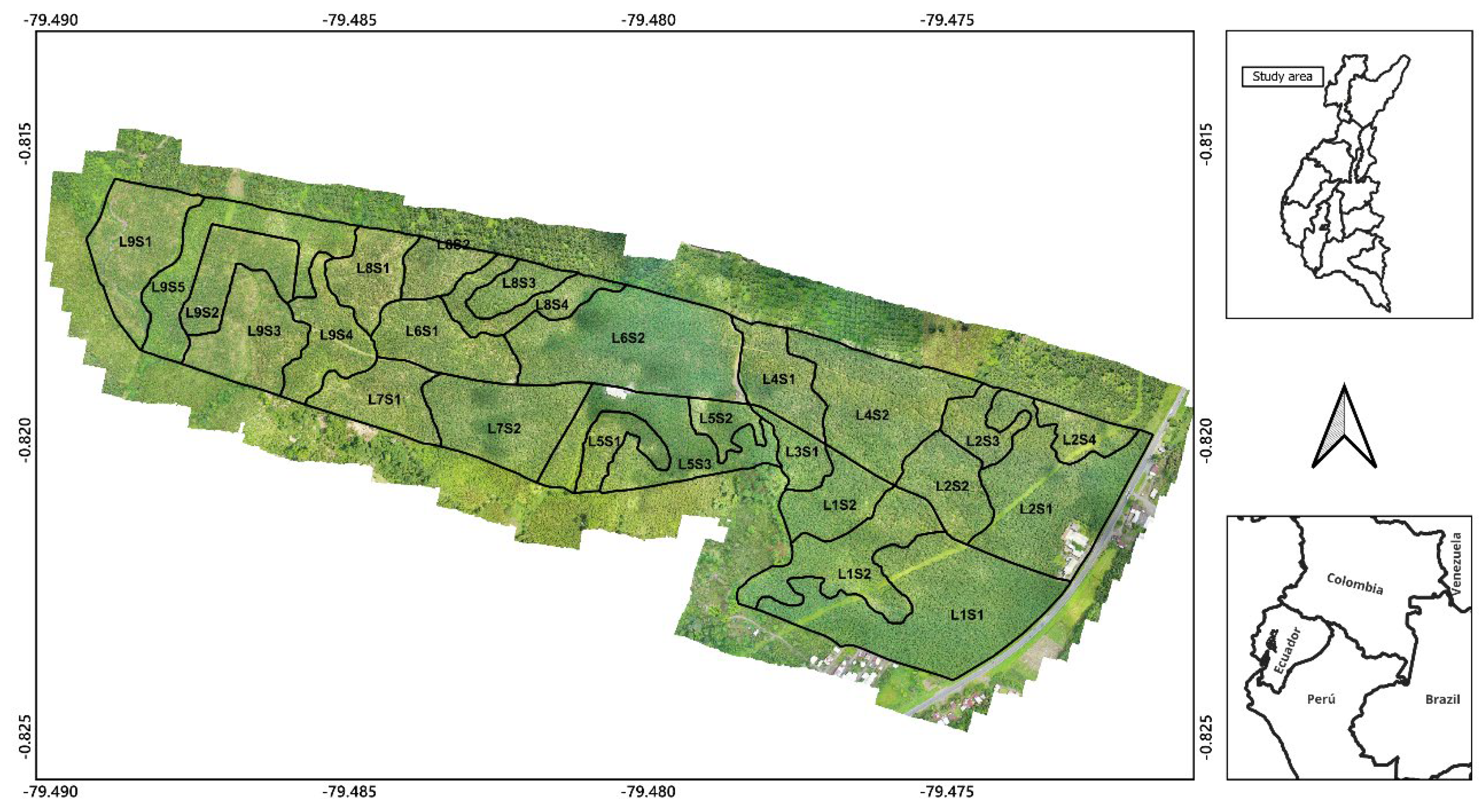
Figure 2.
(top) presents the NDVI map (Normalized Difference Vegetation Index), obtained from multispectral images, which allows identifying variability in plant vegetative vigor. (bottom) shows the digital terrain model (DTM), which represents the topographic variation of the farm.
Figure 2.
(top) presents the NDVI map (Normalized Difference Vegetation Index), obtained from multispectral images, which allows identifying variability in plant vegetative vigor. (bottom) shows the digital terrain model (DTM), which represents the topographic variation of the farm.
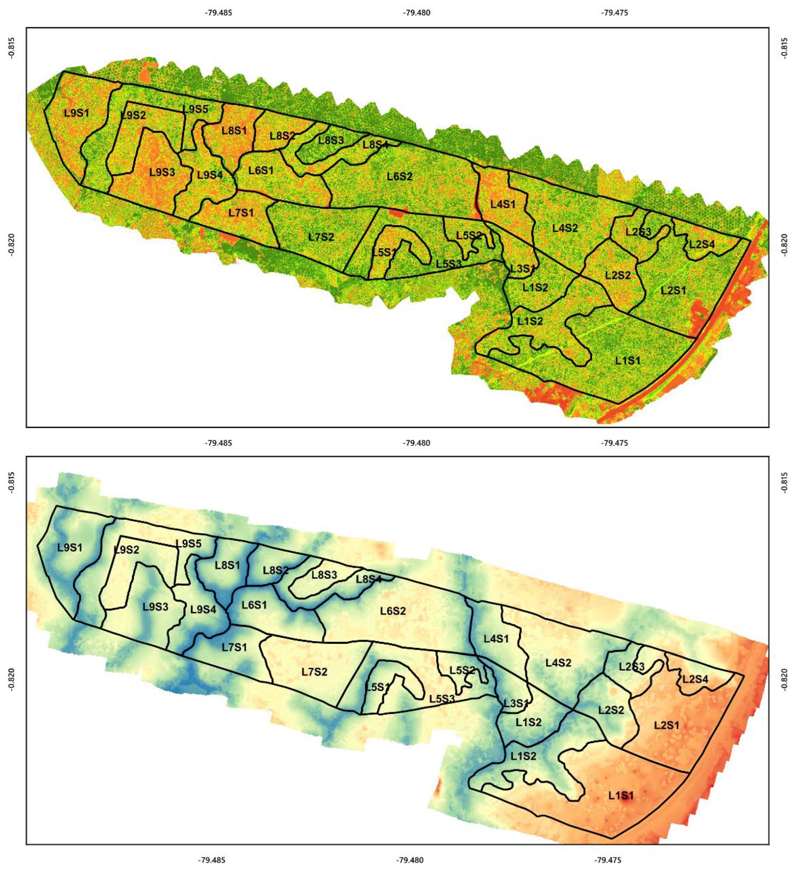
Figure 3.
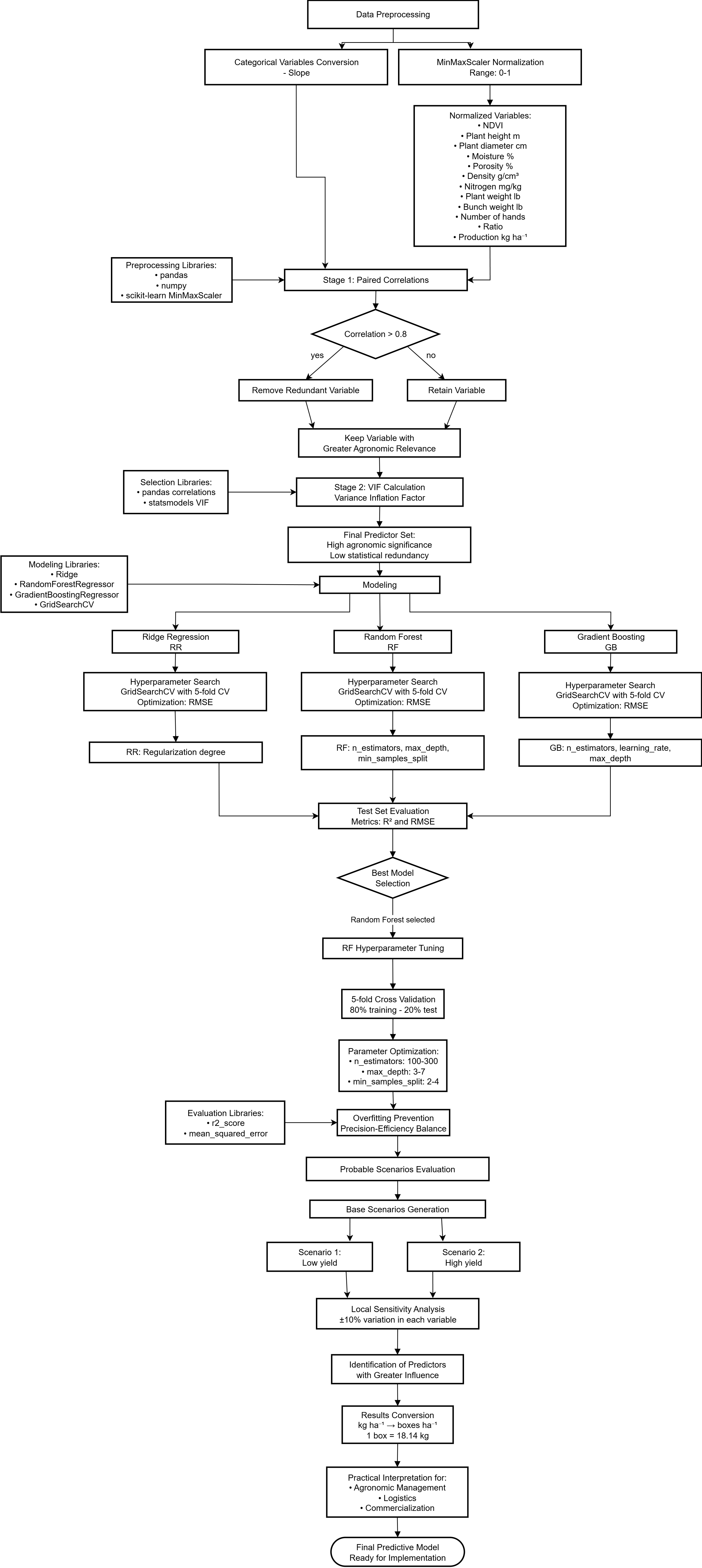
Algorithm for predictive modeling using Machine Learning. The process includes: (1) data preprocessing; (2) variable selection through correlation analysis and VIP projection; (3) training and optimization of multiple algorithms (RR, RF, GB); (4) selection of the best model (Random Forest); (5) sensitivity analysis and applicability in agronomic scenarios for practical management.
Figure 3.
Algorithm for predictive modeling using Machine Learning. The process includes: (1) data preprocessing; (2) variable selection through correlation analysis and VIP projection; (3) training and optimization of multiple algorithms (RR, RF, GB); (4) selection of the best model (Random Forest); (5) sensitivity analysis and applicability in agronomic scenarios for practical management.
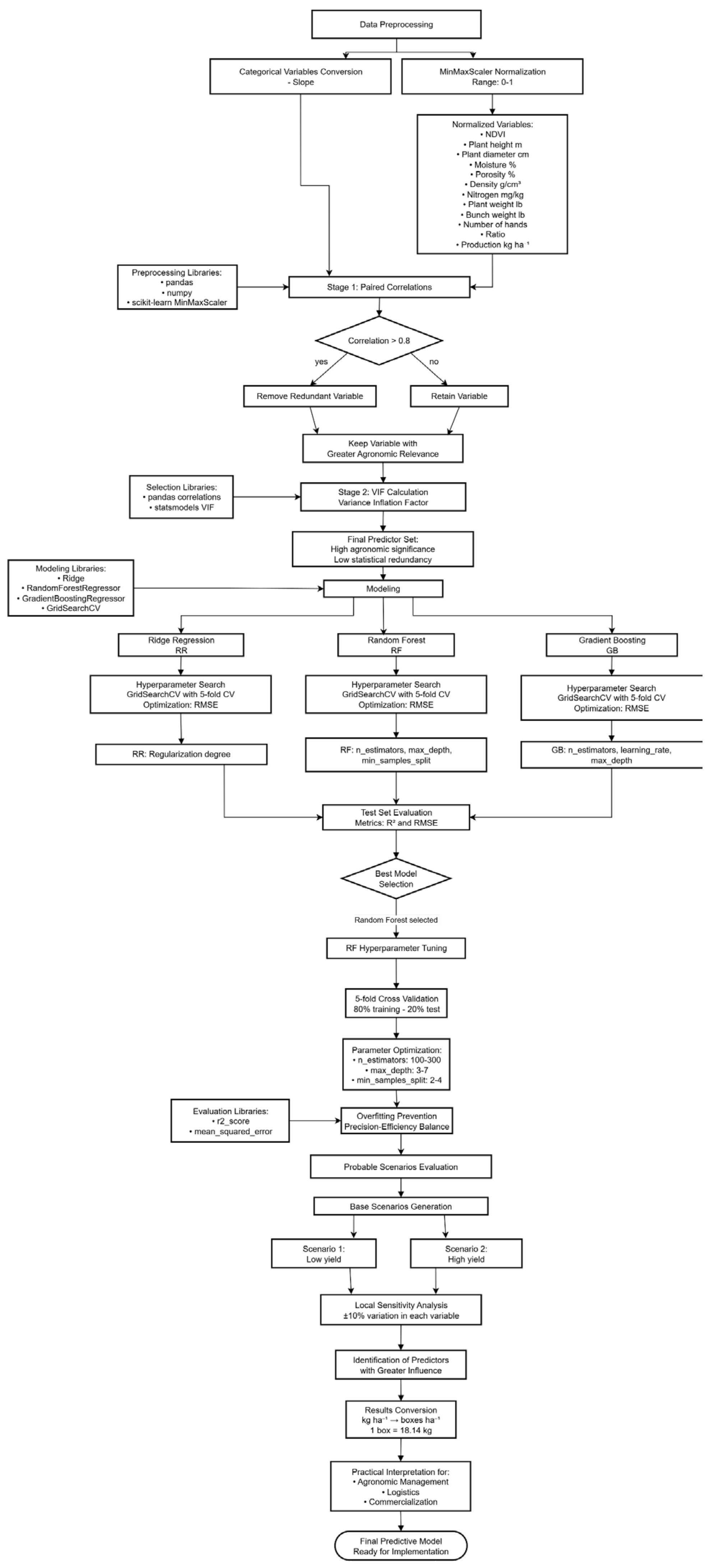
Figure 4.
The figure shows variable importances according to the RF model trained for banana yield prediction, the X axis represents variable importance, and the Y axis represents variables.
Figure 4.
The figure shows variable importances according to the RF model trained for banana yield prediction, the X axis represents variable importance, and the Y axis represents variables.
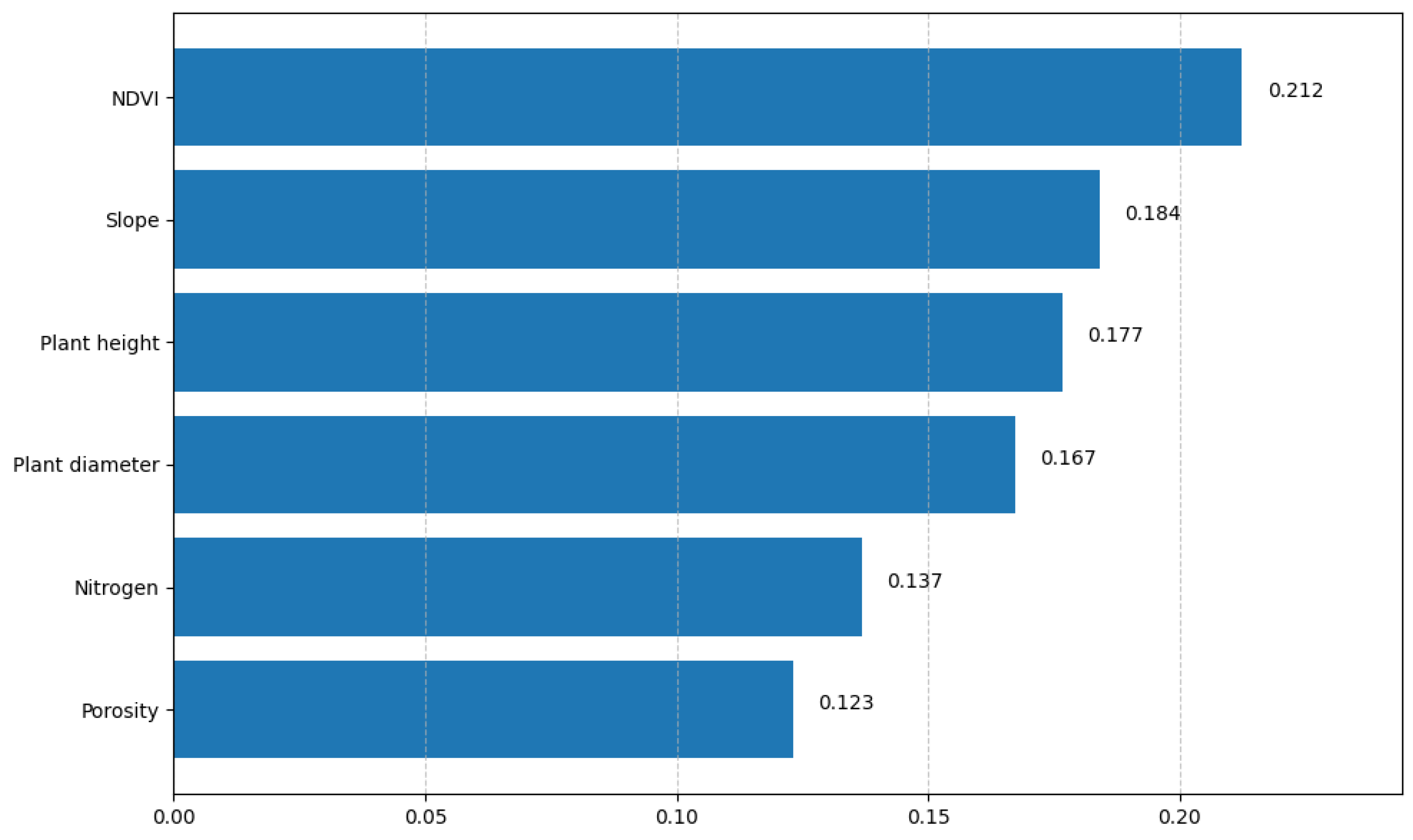
Figure 5.
Residuals vs. predictions from the model, each point is labeled with its plot case; the dashed line indicates zero residual, the X axis represents yield kg ha−1, the Y axis represents residuals. Positive residuals represent underestimations and negative ones overestimations.
Figure 5.
Residuals vs. predictions from the model, each point is labeled with its plot case; the dashed line indicates zero residual, the X axis represents yield kg ha−1, the Y axis represents residuals. Positive residuals represent underestimations and negative ones overestimations.
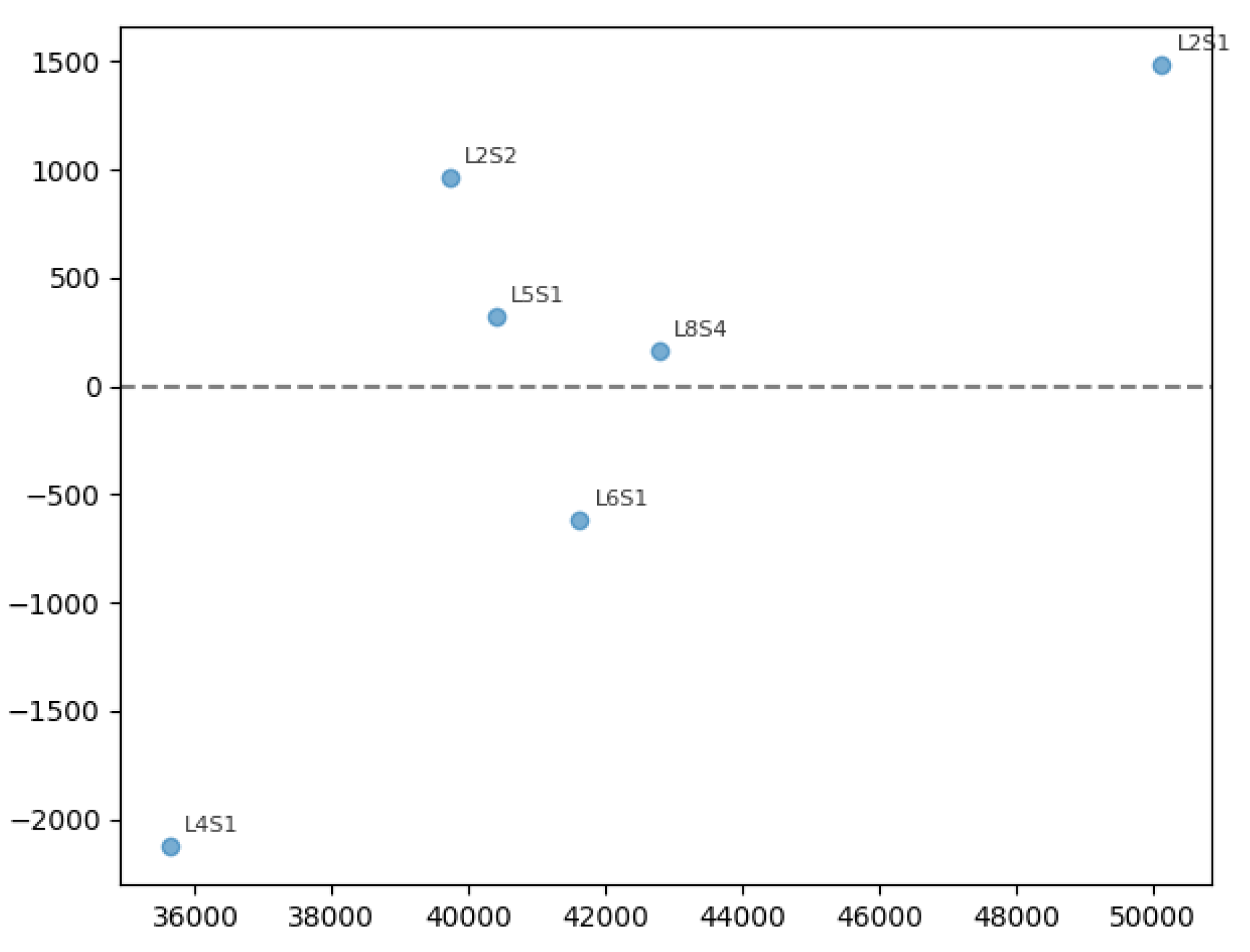
Figure 6.
Relationship between observed and predicted yield by the Random Forest model, the X axis shows measured yield (kg ha−1), the Y axis the estimated, the dashed line is identity (perfect prediction) and the solid line is the best fit line.
Figure 6.
Relationship between observed and predicted yield by the Random Forest model, the X axis shows measured yield (kg ha−1), the Y axis the estimated, the dashed line is identity (perfect prediction) and the solid line is the best fit line.
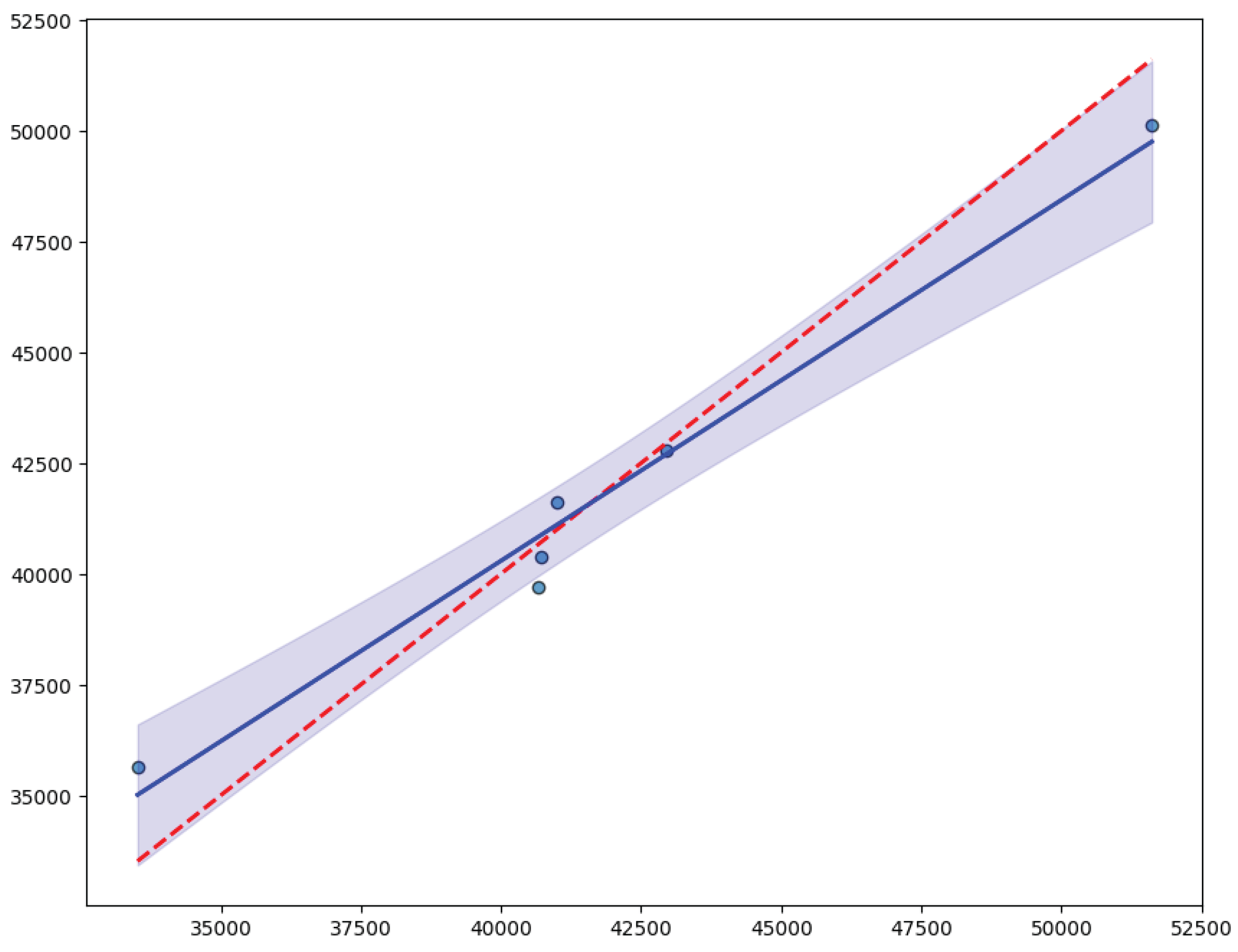
Table 3.
Scenarios represent typical conditions of low and high banana crop yield, evaluation of model predictive performance.
Table 3.
Scenarios represent typical conditions of low and high banana crop yield, evaluation of model predictive performance.
| Yield | NDVI | Height (m) | Diameter (cm) | Nitrogen (%) | Porosity (%) | Slope | Yield (kg ha−1) | Boxes ha-1 |
| Baja | 0.70 | 2.5 | 16.0 | 20 | 30 | 3 | 35,988.5 | 1,983.9 |
| Alta | 0.85 | 4.0 | 25 | 55 | 45 | 1 | 50,571.7 | 2,787.9 |
Table 4.
Sensitivity analysis (±10%) on base scenarios, delta (Δ) response values.
| Yield | Modified variable | Change (%) | yield (kg ha−1) | Δ yield (kg ha−1) | Boxes ha-1 | Δ Boxes ha-1 |
| Low | NDVI | -10% | 35,637.30 | -351.19 | 1,964.57 | -19.36 |
| Low | NDVI | +10% | 36,967.59 | +979.09 | 2,037.90 | +53.97 |
| Low | Height | -10% | 35,988.49 | 0.00 | 1,983.93 | 0.00 |
| Low | Height | +10% | 36,980.12 | +991.63 | 2,038.60 | +54.67 |
| Low | Diameter | -10% | 35,988.49 | 0.00 | 1,983.93 | 0.00 |
| Low | Diameter | +10% | 37,347.32 | +1,358.83 | 2,058.84 | +74.91 |
| Low | Nitrogen | -10% | 35,988.49 | 0.00 | 1,983.93 | 0.00 |
| Low | Nitrogen | +10% | 35,988.49 | 0.00 | 1,983.93 | 0.00 |
| Low | Porosity | -10% | 35,988.49 | 0.00 | 1,983.93 | 0.00 |
| Low | Porosity | +10% | 36,920.1 | +268.67 | 1,998.74 | +14.81 |
| High | NDVI | -10% | 48,025.58 | 2,647.50 | -2,546.10 | -140.36 |
| High | NDVI | +10% | 50,571.68 | 2,787.85 | 0.00 | 0.00 |
| High | Height | -10% | 50,571.68 | 2,787.85 | 0.00 | 0.00 |
| High | Height | +10% | 50,571.68 | 2,787.85 | 0.00 | 0.00 |
| High | Diameter | -10% | 50,571.68 | 2,787.85 | 0.00 | 0.00 |
| High | Diameter | +10% | 50,571.68 | 2,787.85 | 0.00 | 0.00 |
| High | Nitrogen | -10% | 49,256.46 | 2,715.35 | -1,315.2 | -72.50 |
| High | Nitrogen | +10% | 50,571.68 | 2,787.85 | 0.00 | 0.00 |
| High | Porosity | -10% | 50,135.07 | 2,763.79 | -436.61 | -24.07 |
| High | Porosity | +10% | 50,571.68 | 2,787.85 | 0.00 | 0.00 |
Disclaimer/Publisher’s Note: The statements, opinions and data contained in all publications are solely those of the individual author(s) and contributor(s) and not of MDPI and/or the editor(s). MDPI and/or the editor(s) disclaim responsibility for any injury to people or property resulting from any ideas, methods, instructions or products referred to in the content. |
© 2025 by the authors. Licensee MDPI, Basel, Switzerland. This article is an open access article distributed under the terms and conditions of the Creative Commons Attribution (CC BY) license (http://creativecommons.org/licenses/by/4.0/).
Copyright: This open access article is published under a Creative Commons CC BY 4.0 license, which permit the free download, distribution, and reuse, provided that the author and preprint are cited in any reuse.


