
Submitted:
04 September 2025
Posted:
10 September 2025
You are already at the latest version
Abstract
This work proposes a structural foundation for the universal laws of multi-scale complexity introduced by Siegenfeld and Bar-Yam (Entropy, 2025). Their formulation describes the complexity profile, the multi-scale law of requisite variety, and the sum rule as phenomenological regularities, but leaves their physical origin unspecified. Here we interpret these laws as consequences of a phase-topological principle: the minimal action bound for distinguishability, δS ≥ ħ. Within this framework, three structural results follow: (i) a capacity bound limiting the number of coherent supports in a region by its available action budget, corresponding to the requisite variety condition; (ii) a balance principle showing that the total action budget provides a fixed constraint that can be redistributed across scales, underlying the sum rule; and (iii) a projection rule expressing the phenomenological complexity profile as the per-scale entropy increments of a structural distinction measure. Together, these results suggest that phenomenological complexity laws emerge as consequences of a single action principle, analogous to how thermodynamic irreversibility arises from statistical mechanics. By explicit analogy with Landauer’s bound for erasure, we interpret ħ as the minimal action cost of distinction, providing a possible structural route toward unifying complexity science with the broader physical context of quantized action and finite informational capacity.
Keywords:
multi-scale complexity
; requisite variety
; sum rule
; action principle
; Planck’s constant
; Landauer bound
; symplectic topology
; quantum speed limits
; structural invariants
1. Introduction: From the Cost of Erasure to the Cost of Distinction
1.1. Conceptual Anchor: Maxwell’s Demon
The deep link between information and physics was crystallized by Maxwell’s Demon and its resolution via Landauer’s principle [1]: erasing one bit of information has an irreducible thermodynamic cost of . Subsequent developments in the thermodynamics of computation [2,3] established a rigorous association between erasure and energetic expenditure. Independent lines of work—from Bekenstein’s geometric entropy bounds [4] to Zurek’s decoherence program [5]—further reinforced that information is constrained by physical law.
Here we propose to interpret Planck’s constant ℏ as the minimal quantum of action required for a physical distinction to be sustainably realized,1 in contrast to the statistical cost of erasure. This lower bound is structural and originates in phase-topological consistency conditions. In geometric quantization, these conditions appear as integrality of the symplectic flux,
with the symplectic form on phase space [6,7,8]. Equivalently, the cohomology class is integral, ensuring globally consistent phase holonomies. We note that the canonical flux quantum is ; throughout this paper we adopt ℏ as the operative unit for sustainable distinction. In this sense, the unit that protects coherent distinctions is anchored in topology rather than in statistical mechanics.
1.2. The Problem of Complexity and a Proposed Framework
Recent advances in complexity science identify robust multi–scale regularities. The framework of Siegenfeld and Bar–Yam [9,10] formalizes a complexity profile, a multi–scale law of requisite variety, and a sum rule. These are presented as phenomenological regularities, leaving their physical origin unspecified.
To address this gap, we develop a two–level architecture that links phenomenology to structural constraints:
- Phenomenological level: information–theoretic descriptors (complexity profile, multi–scale requisite variety, sum rule) [11];
- Structural level: a symplectic–topological formulation in which constraints follow from a minimal–action requirementwhere is the Poincaré–Cartan one–form and is a closed cycle in phase space.
This architecture parallels the relation between Thermodynamics and Statistical Mechanics: macroscopic laws emerge from microscopic structure [12]. In our formulation, the inequality is taken as an operational formulation of the underlying quantization dictated by geometric integrality.
2. Formalism of the Phase-Topological Framework: Foundations
2.1. Coherence Principle and Minimal Units
Definition 1
(Coherence Principle). For any physically distinguishable closed cycle γ in phase space,
where is the canonical Poincaré–Cartan one-form of the action. A minimal coherent unit is any configuration saturating this inequality, .
Note. Here denotes the line integral of over a closed trajectory, not a variational derivative in the Euler–Lagrange sense.
This condition is adopted here as a working structural postulate of the framework. The interpretation is operational: every sustainably realized distinction requires at least one quantum of action, meaning that it preserves phase coherence sufficiently to correspond to an (approximately) orthogonal support in Hilbert space.
The structural origin of this postulate lies in geometric quantization. The holonomy of the prequantum bundle, together with the Maslov index correction, imposes the Bohr–Sommerfeld quantization rule,
for any closed curve on a Lagrangian submanifold of phase space, where is the Maslov index [8,13,14]. This quantization condition ensures the global consistency of phase holonomies. In our reformulation, it is interpreted as a minimal-action requirement for the sustainability of distinct physical configurations.
The role of the dynamical component in the Poincaré–Cartan form will be analyzed in later sections and appendices, where explicit Hamiltonian evolutions and quantum speed-limit bounds are discussed (Appendix A). For now, the principle is established at the level of structural consistency.
2.2. Measure of Distinction
To quantify the effective number of reliably distinguishable configurations, we introduce the structural measure:
- For a finite set of pure states U:i.e. the dimension of the subspace spanned by U. For non-orthogonal sets this counts the linear span, not the number of reliably distinguishable states.
- For a mixed state with density operator :where is the von Neumann entropy. This definition, sometimes referred to as the exponential of the entropy, interprets as an effective Hilbert space dimension, consistent with approaches to typical entanglement and effective dimension in quantum statistical mechanics [15,16].
Throughout we use the natural logarithm, so is expressed in nats; using would instead yield bits. A fundamental property of this measure is subadditivity under composition of subsystems: for two subsystems A and B within a fixed context,
This inequality follows directly from the subadditivity of the von Neumann entropy:
and therefore
Equality holds for product states, while strict inequality arises in the presence of correlations or entanglement. This expresses the structural limitation that the number of jointly sustainable distinctions cannot exceed the available resource budget. In later sections we show how this information-theoretic property is connected to the coherence bound ; the two are not independent assumptions but complementary expressions of the same structural limitation, linked explicitly in subsequent theorems.
3. Results: Structural Derivation of Complexity Laws
3.1. Multi-Scale Law of Requisite Variety
Theorem 1
(Capacity Bound). The number of mutually orthogonal coherent units that can be sustained in a region R is bounded above by the available action budget:
Here is defined as the supremum of the action integral over all relevant closed cycles contained within the spacetime region R,
This definition ensures that is well-posed and consistent with the geometric setting. The inequality follows directly from the coherence principle: each coherent unit requires at least one quantum of action to remain stable. Hence the number of reliably distinguishable configurations cannot exceed the ratio .
Clarification. In geometric quantization the elementary flux quantum is ; here we adopt ℏ as the operational threshold for sustainable distinction. This should be understood as the minimal action cost of distinguishability, not as a literal Bohr–Sommerfeld spacing. The bound of Theorem 1 may be further restricted by the finite Hilbert-space dimension of the system, as discussed in Appendix A.
Connection to Phenomenological Laws.
In the framework of Ref. [9], the multi-scale law of requisite variety requires that the system complexity must not fall below that of the environment, , for all scales n. The capacity bound provides the corresponding structural resource constraint: if system X has a smaller action budget than needed to encode the states of its environment Y, then necessarily for some scales. This is best interpreted as a structural limitation underlying Ashby’s law, not a literal proof of its full phenomenological formulation.
3.2. Sum Rule
Principle 2
(Balance of the Action Budget). The total action budget associated with a region R provides a fixed upper bound on the system’s informational capacity. This budget remains constant under redistribution of coherent structures, provided the region and its boundary conditions are fixed. While the distribution of complexity may shift between microscopic and macroscopic scales, the overall budget does not change.
This expresses that action functions as a finite resource: a system may allocate its budget to many small-scale distinctions or to fewer large-scale correlated structures, but the total capacity remains constrained by .
Connection to Phenomenological Laws.
The sum rule of Ref. [9],
is interpreted here as the phenomenological projection of this balance principle. The right-hand side, , represents the total information capacity of the system’s components, structurally bounded by the fixed action budget .
Illustrative Example.
In a spin chain, the same budget can be allocated in two limiting ways: (i) into N independent coherent units (a microscopic peak of complexity), or (ii) into a single highly entangled GHZ-type configuration (a macroscopic peak). Both respect the same resource bound, though the distribution of across scales differs. In both cases one finds , consistent with the budget constraint.
3.3. Complexity Profile and the Distinction Measure
Theorem 3
(Projection of Distinction). For a coarse-grained system, the phenomenological complexity profile can be expressed as the per-scale increment of the structural distinction measure:
where denotes the coarse-graining operator at resolution scale n, modeled as an entropy non-decreasing channel such as a conditional expectation (pinching) onto the subalgebra corresponding to scale n. Here refers to the coarsest-graining operator, corresponding to the maximal available scale.
This definition guarantees whenever each coarse-graining step is entropy non-decreasing. In typical systems the profile decays with scale, consistent with phenomenological observations, though local fluctuations may occur. The telescoping sum
ensures consistency with the action budget constraint.
We emphasize that the entropic formulation given above is taken as the primary definition of the complexity profile. The combinatorial model of Appendix B serves as an illustrative discrete analogue; their equivalence holds under canonical coarse-graining, as discussed in Appendix C.
3.4. Conclusion
Within this formulation, the phenomenological laws of complexity—the multi-scale law of requisite variety, the sum rule, and the scale-dependent complexity profile—can be interpreted as emergent consequences of a single structural action principle, rather than as independent postulates.
Schematic Correspondence of Structural Results
Figure 1.
Correspondence between structural principles (left/middle) and phenomenological laws of multi-scale complexity (right). Dashed arrows indicate the projection of structural results into phenomenological formulations.
Figure 1.
Correspondence between structural principles (left/middle) and phenomenological laws of multi-scale complexity (right). Dashed arrows indicate the projection of structural results into phenomenological formulations.
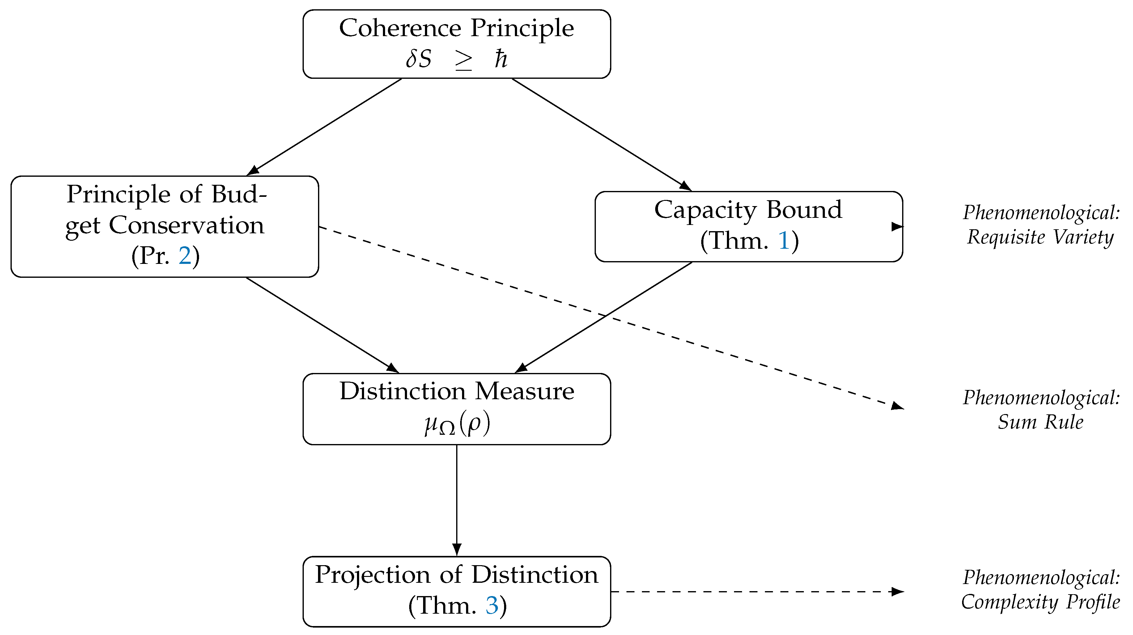
This diagram highlights the logical structure: the Coherence Principle generates both the Capacity Bound and the Balance principle. Together with the distinction measure, they underlie the projection theorem, from which the phenomenological complexity laws follow.
4. Discussion
The results presented above suggest that the phenomenological laws of multi-scale complexity can be interpreted as emergent quantum-informational consequences of a single structural principle of action. This section outlines broader implications of this finding, ranging from reinterpretations of foundational concepts in physics to potential applications in quantum information, cybernetics, and the philosophy of science.
4.1. The Phase-Topological Framework as the “Statistical Mechanics” of Complexity
The analogy between the two-level framework proposed here and the relationship between Statistical Mechanics and Thermodynamics, introduced in Section 1, can now be made more precise. The results in Section 3 provide a formal bridge between these two levels. The laws of multi-scale complexity, as formulated by Siegenfeld and Bar-Yam [9], function as macroscopic, phenomenological rules governing the distribution of information in complex systems. The framework developed here provides a microscopic, structural foundation for these rules.
The Capacity Bound and the Principle of Budget Conservation are not postulated information-theoretic laws but physical constraints grounded in the symplectic-topological properties of the underlying phase space. Thus, the universal laws of complexity may be viewed as emergent quantum-informational laws, in parallel with how the laws of thermodynamics arise from the microscopic mechanics of constituent systems [10,12,17,18].
Earlier formulations of multiscale complexity and requisite variety [19,20] introduced these ideas descriptively. The present framework provides a structural origin, suggesting that what has been observed phenomenologically as “laws of complexity” may be interpreted as consequences of a more primitive constraint: the minimal action bound , where is defined as in Section 3.
4.2. Reinterpreting Maxwell’s Demon through the Action Cost
The classic thought experiment of Maxwell’s Demon illustrates the deep connection between information and thermodynamics. Landauer’s principle resolved the paradox by identifying the thermodynamic cost of erasing information [1,2,3]. Within the present framework, we interpret each act of establishing a physical distinction as requiring at least one quantum of action, ℏ. Therefore, the demon’s ability to decrease entropy is limited not only by the thermodynamics of its memory but, more fundamentally, by the available action budget required to perform distinctions. This limitation may be regarded as phase-topological in nature, representing the cost of establishing information rather than merely erasing it. From this perspective, Ashby’s law of requisite variety [21] can be situated in a broader physical context.
4.3. Broader Implications
Quantum Information and Holography.
The Capacity Bound
establishes a fundamental limit on the number of distinguishable states that can be supported within a region defined by its available action. This resonates with holographic principles, such as the Bekenstein bound [4], which constrain the information content of a region in terms of its geometric properties. The present work suggests a possible connection between the action budget of a spacetime region and its geometric information bounds, though this analogy remains speculative and requires further investigation.
Biology and Cybernetics.
Ashby’s Law of Requisite Variety, a cornerstone of cybernetics [21], states that an effective regulator must have at least as much variety as the system it controls. The multiscale version of this law, as articulated by Siegenfeld and Bar-Yam [9], may find a possible physical grounding in the action framework. The requirement for a system to possess sufficient variety corresponds to the requirement of having a sufficient action budget to sustain the needed distinctions. This aligns with recent studies of complexity matching and eco-evolutionary dynamics [22,23], suggesting that cybernetic principles may be physically constrained by available action resources.
Philosophy of Science.
The framework developed here is consistent with structural realist interpretations of scientific theories [24,25]. What appears fundamental, within this framework, are not individual objects (particles, fields) but the structural constraints—action principles, topological quantization rules—from which observable entities emerge as stable, distinguishable configurations. This perspective resonates with Anderson’s dictum that “more is different” [17] and with the view that emergent macroscopic laws require structural explanation rather than independent postulation.
Dynamics versus Constraints.
It is important to note that the present framework primarily defines the structural constraints and the space of possibilities for complexity profiles, as dictated by the action budget. The specific dynamics, governed by a system’s Hamiltonian, determine which particular profile is realized within these bounds. In other words, the constraints define the feasible set, while the dynamics select the actual trajectory. A detailed study of this interplay represents a promising direction for future research.
The structural principles derived above can be summarized in a compact chain of correspondences:

Table 1.
Correspondence between the phenomenological laws of Siegenfeld–Bar-Yam (Entropy, 2025) and the structural phase-topological framework developed here.
Table 1.
Correspondence between the phenomenological laws of Siegenfeld–Bar-Yam (Entropy, 2025) and the structural phase-topological framework developed here.
| Phenomenological Law | Structural Foundation (This Work) | Interpretation |
|---|---|---|
| Multi-scale law of requisite variety: for all n. | Capacity Bound:. | The system cannot sustain more distinctions than allowed by its action budget. If , then necessarily follows for some scales. |
| Sum rule:. | Principle of Budget Conservation: provides a fixed upper bound under redistribution across scales (with fixed boundary conditions). | Redistribution of complexity across scales reflects the balance of the total action budget, while the total informational capacity remains constrained by . |
| Complexity profile . | Projection of Distinction:. | The profile can be interpreted as a finite-difference projection of the structural measure under hierarchical coarse-graining, rather than as an independent fundamental law. |
This correspondence emphasizes that the complexity laws described in Ref. [9] should not be treated as independent postulates. Instead, they can be interpreted as quantum-informational consequences of a deeper structural principle: the minimal action cost of distinction.
5. Conclusions
The results of this work can be summarized as follows: the minimal action bound defines a bounded capacity for distinctions; this bounded capacity can be interpreted as giving rise to structural contextuality in the relations between system and environment; and from this structural contextuality the universal laws of multi-scale complexity can be understood to emerge.
Within this framework, Planck’s constant may be understood as the minimal quantum of action required to sustain distinguishable configurations. The coherence bound enforces a finite capacity for distinctions, providing, within this framework, a structural account of contextuality in system–environment interactions and supporting the appearance of the phenomenological laws of multi-scale complexity as formulated by Siegenfeld and Bar-Yam.
The framework developed here suggests a foundation for complexity theory analogous to the role of statistical mechanics in thermodynamics. What Siegenfeld and Bar-Yam formulated phenomenologically — the multi-scale law of requisite variety, the sum rule, and the complexity profile — can be interpreted as emergent consequences of a single structural principle: the minimal action cost of distinction.
By grounding these laws in a phase-topological principle, the present formulation offers a possible structural route toward integrating complexity science with the broader physical framework of quantized action and finite informational capacity.
Appendix A. Action Budget for a Spin Chain
Explicit Calculation of M max (R) for a System of N Qubits
We specialize the coherence principle to a spin chain. Consider a chain of N qubits, each represented by a localized coherent unit with minimal action cost
The total chain is described by the tensor product Hilbert space
Action budget.
Let R be a finite spacetime region (a world-tube) in which the spin chain is embedded. We define the available action budget as the supremum of the action line integral over all relevant closed cycles contained within R:
With fixed boundary conditions (no external change of drive/controls at ), the coherence principle implies
where is the maximal number of mutually orthogonal states sustainable in R. Hence,
Consistency with Hilbert space capacity.
Since the Hilbert space dimension is finite,
Therefore,
Entropy bound.
For any mixed state supported on the chain,
where the logarithm is taken in base e (nats). Using instead would yield the bound in bits. Thus the distinguishability capacity is limited by the available action budget.
Dimensional check.
and ℏ have the same units of action, so is dimensionless, consistent with its interpretation as a maximal count.
Operational Estimate via the Hamiltonian
Consider a uniform nearest-neighbor Hamiltonian
with coupling constant J (energy scale). For evolution over , when spatial boundary terms are negligible, the dominant contribution to arises from the temporal component:
For the ZZ Hamiltonian the local terms commute and
Combining with (A4) gives the operational bound
Variants.
- For XX/XY nearest-neighbor models one still has the triangle-inequality estimate , yielding under bounded local strengths. - For a homogeneous field , , hence
- More generally, for any local Hamiltonian with bounded interaction strength, the action budget scales at most linearly with N and with T.
Interpretation.
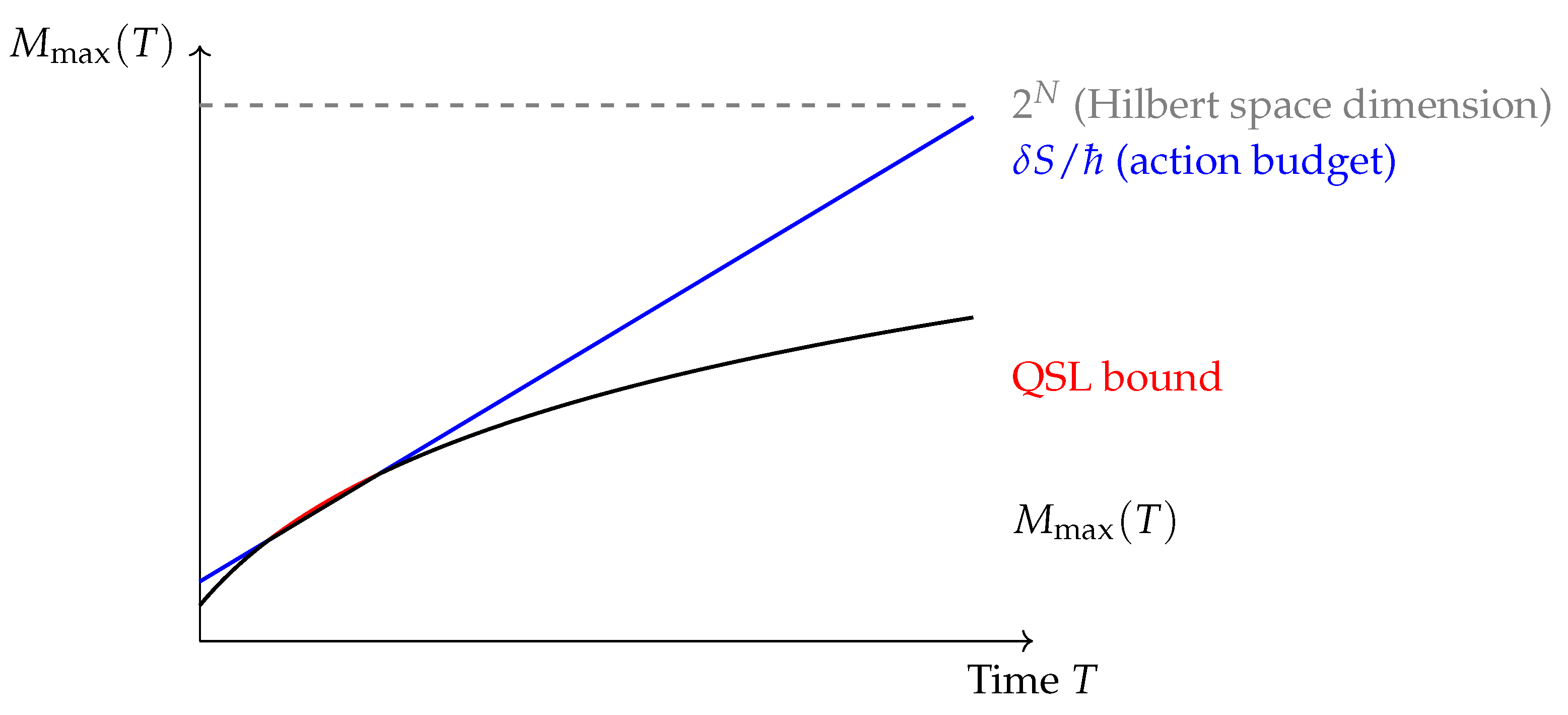
Two independent ceilings control the number of distinct coherent states producible in time T: (i) the Hilbert-space ceiling ; (ii) the action ceiling . Thus the coherence condition manifests as a bound on the number of orthogonalizations achievable within a finite window.
Connection to Quantum Speed Limits
For a time-dependent Hamiltonian , the minimal orthogonalization time obeys the Mandelstam–Tamm and Margolus–Levitin bounds [26,27]:
where is the instantaneous energy variance and is the mean energy above the ground state. Integrating over time,
Heuristically, each orthogonalization carries an action cost of order ; the precise constants depend on the fidelity threshold adopted in projective Hilbert space. These bounds should therefore be read as asymptotic ceilings, consistent with the resource inequality .
Schematic Bound Comparison
Figure A2.
Three ceilings limiting the number of orthogonal states in a spin chain. The Hilbert-space ceiling (gray dashed), the action-budget ceiling (blue), and the quantum-speed-limit ceiling (red) jointly constrain (black). Curves illustrative, not to scale.
Figure A2.
Three ceilings limiting the number of orthogonal states in a spin chain. The Hilbert-space ceiling (gray dashed), the action-budget ceiling (blue), and the quantum-speed-limit ceiling (red) jointly constrain (black). Curves illustrative, not to scale.
Appendix B. Demonstration of the Sum Rule
This appendix illustrates the structural content of the Sum Rule (Principle 2) on explicit many-body states.
Profiles C X (n) for Product vs. GHZ States Under the Same δS Budget
Setting and budget of action.
Consider a chain of N qubits realized as N localized coherent units, each corresponding to one sustainable degree of freedom in Hilbert space. The coherence threshold implies that each stable support requires at least one quantum of action:
Fix a spacetime region R sustaining the chain with total action budget , defined invariantly through the Poincaré–Cartan one-form as
taken over all admissible closed cycles under fixed boundary conditions and process duration T (cf. Appendix A). Set
We assume , so that all N units can be sustained.
Multiscale profile (combinatorial definition).
Define a dependency hypergraph on X by placing a (hyper)edge on any subset () whenever the joint state exhibits nontrivial correlation across A (e.g. nonzero mutual information in the chosen ensemble/context). Let be the connected components of with sizes (so ). For define the complexity profile
Intuitively, counts how many independent coherent components extend to scale . This discrete, graph-based definition is used here as an illustrative analogue; the entropic formulation given in Appendix C is the primary structural definition.
Sum Rule (discrete form).
The profile (A15) satisfies the exact identity
Proof. Each component of size contributes 1 to for every and contributes 0 otherwise; summing over n yields , then summing over i yields N.
Action–profile correspondence.
Since each coherent unit costs at least ℏ, one has
Let denote the action accumulated along the realized closed trajectory . By budget additivity for the realized process,
Hence the chain of inequalities
Thus, when the sustained number of units equals N, the budget version of the sum rule reads
If the available budget only sustains units (e.g. sparse activation), the same construction restricted to the active units yields .
Two extremal architectures under the same δS budget
(A) Product register (independent local DOF).
The dependency hypergraph has no edges; all vertices are isolated. Hence the connected components are with sizes . By (A15),
and the sum rule gives .
(B) GHZ architecture (global DOF).
For the GHZ ensemble, the dependency hypergraph is fully connected (, ). Thus,
and .
Same action, different profiles.
Both architectures use the same unit budget , but allocate distinguishability across scales differently:
Quantum–Informational Check
For the product register, for all . For the GHZ ensemble, (in nats; equals 1 bit under ) for every nontrivial bipartition. Thus the combinatorial profile above is consistent with the quantum mutual-information criterion used to define edges.
Units and dimensional check.
is dimensionless (a pure count). The budget constraint enters only through the number of sustained units,
providing a dimensionless bound, consistent with being a pure count.
General Remark: Redistributing a Fixed δS
Given a fixed action budget , one may trade local variety for global coordination without changing : independent registers concentrate at , while globally entangled architectures (like GHZ) spread flatly across all n. This is the operational content of the Sum Rule under the coherence budget.
(C) Block–GHZ (“clustered”) architecture.
Partition X into m blocks of size L, so . On each block prepare an L-qubit GHZ state:
The hypergraph has m connected components of sizes . Therefore,
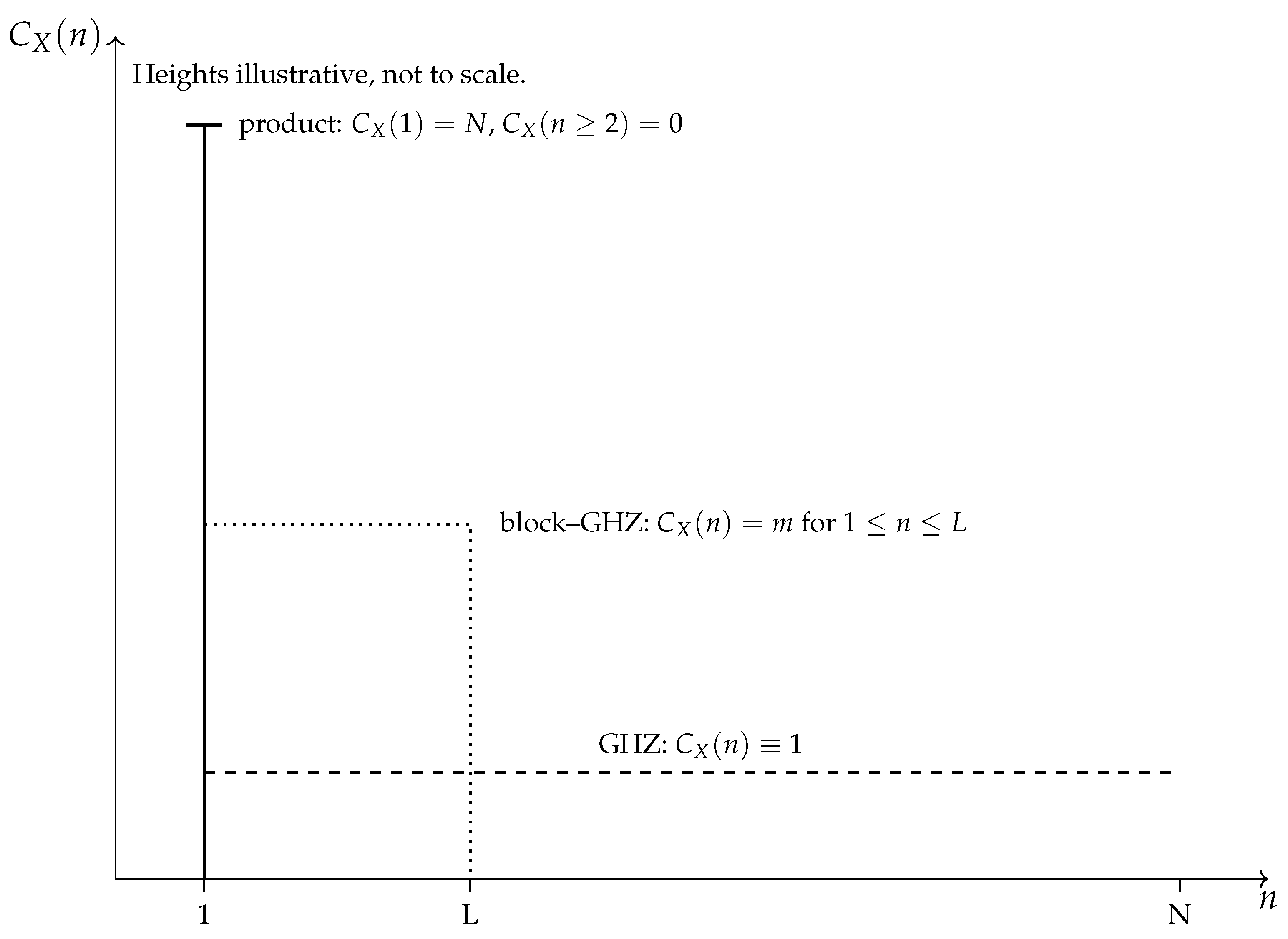
which interpolates between product () and GHZ ().
Remark on graph and cluster states.
For a connected graph state, the hypergraph defined by unconditional correlations is connected, yielding . In a specific measurement context (stabilizer readout), one obtains effective finite correlation length, producing a plateau in followed by decay. This context dependence is consistent with structural contextuality, while the Sum Rule and the action budget constraint
remain intact.
Schematic Profiles (Product / Block–GHZ / GHZ)
Figure A3.
Complexity profiles for product (“needle”), block–GHZ (“plateau”), and GHZ (flat line at 1). Different allocations of the same action budget correspond to different shapes of the profile, but the discrete area under each profile is invariant and equals N.
Figure A3.
Complexity profiles for product (“needle”), block–GHZ (“plateau”), and GHZ (flat line at 1). Different allocations of the same action budget correspond to different shapes of the profile, but the discrete area under each profile is invariant and equals N.
Note on summation convention.
In the combinatorial formulation used here, the sum in Eq. (A16) runs to N, while in the entropic formulation of Appendix C it runs to (since the last coarse-graining step to contributes trivially). The two conventions are equivalent up to this endpoint.
Appendix C. Proof of Theorem 3
Statement of Theorem 3
Theorem 3 asserts that for a coarse–grained system, the phenomenological complexity profile can be identified with the per–scale logarithmic increment of the structural measure of distinction:
where denotes the coarse–graining operator acting at scale n, and is the density operator of the system. Throughout we use the natural logarithm (units: nats); using yields the same statements in bits up to a constant factor. We work with a finite chain of scales , where is the finest and is the coarsest coarse–graining.
Hierarchical decomposition
Consider a system organized into nested scales of resolution:
A coarse–graining at scale n is represented by a map
modeled as a conditional expectation (a pinching / entropy non–decreasing channel) onto a von Neumann subalgebra that captures observables resolvable at scale n. The algebras form a decreasing chain
so that is strictly coarser than . Operationally, discards distinctions below scale n, ensuring a consistent coarse–graining chain
Structural measure of distinction
For a mixed state , define
Under coarse–graining,
Monotonicity
For conditional expectations (and, more generally, pinching maps / entropy non–decreasing channels), the von Neumann entropy is monotone non–decreasing (Uhlmann, Araki):
Consequently,
and the per–scale increments
are non–negative.
Equivalence Under Canonical Coarse–Graining
The phenomenological profile of Siegenfeld–Bar–Yam counts distinctions persisting at scale . Under canonical coarse–graining procedures that respect the dependency partition of the system (cf. Appendix B)—i.e., conditional expectations that collapse each dependency component to a single effective degree of freedom for n below its size and to a trivial one above—the operational content of “persisting distinctions” coincides with the finite–difference loss of distinguishability:
This provides the claimed identification in the class of canonical coarse–grainings used throughout the paper.
Entropy–Action Bound and Completion of the Proof
We now complete the bridge to the action budget and ℏ.
Lemma C.1 (Entropy bounded by capacity).
Let R be a spacetime region with action budget and let be the maximal number of mutually orthogonal states that can be sustained in R (Theorem 1). Then for any state supported in R and for any scale n,
Proof. Write , , with orthonormal. By definition of , no ensemble of more than mutually orthogonal states can be sustained in R. Hence , giving . □
Theorem C.2 (Action–profile bound).
For any canonical coarse–graining chain as above and any initial state supported in R,
Proof. The first equality is the telescoping sum of per–scale increments. By Lemma C.1, and , giving the first inequality. The second follows from Theorem 1. The last step uses for , with . □
Remark (Tightness).
The logarithmic bound is tighter; the final linear bound is a convenient but coarse estimate.
Corollary C.3 (Bits version).
With ,
Conclusion
Theorem 3 identifies with the per–scale entropy increments of the structural measure under canonical coarse–graining. Lemma C.1 and Theorem C.2 complete the proof by bounding the total profile in terms of the structural action budget : the sum cannot exceed (and therefore is ). Hence the phenomenological profile is not only equivalent to entropy increments but also structurally constrained by the minimal action principle.
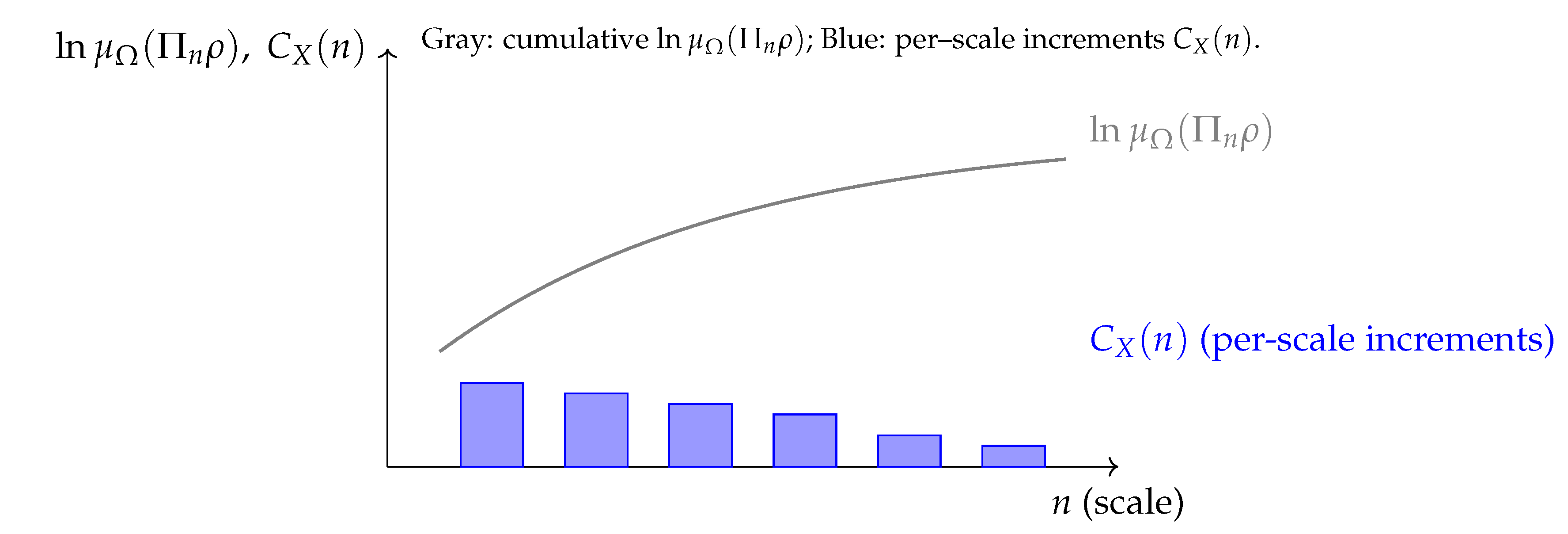
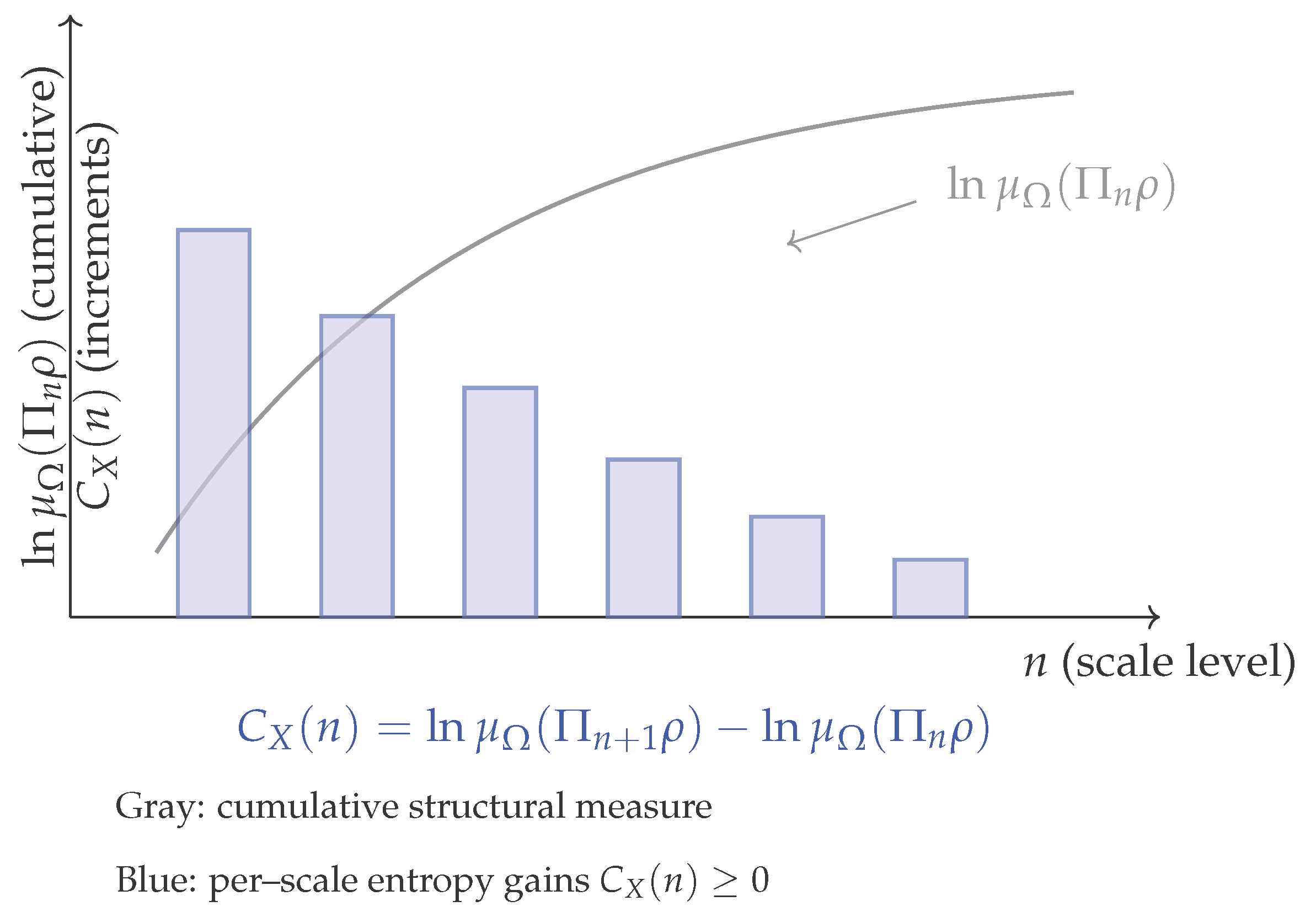
Figure A4.
Schematic illustration of Theorem 3. The gray curve shows the cumulative distinction measure , which increases monotonically with the scale n under canonical coarse–graining. The blue bars represent the finite differences , which are nonnegative and whose discrete sum is bounded by . Heights illustrative, not to scale.
Supplementary Note: Monotonicity of Entropy under Canonical Coarse–Graining
At first sight, there appears to be a tension between two statements: on the one hand, the von Neumann entropy under canonical coarse–graining is known to be monotonically increasing (Uhlmann [28], Araki [29]); on the other hand, the phenomenological complexity profile of Siegenfeld–Bar–Yam is monotonically decreasing with scale. This is not a contradiction, because the two quantities refer to different levels of description. The entropy is a cumulative measure, growing as distinctions are discarded, while the profile is defined by the finite differences of this entropy between successive scales. The construction below makes this relation explicit and identifies the profile as the sequence of per–scale entropy gains (equivalently, information losses).
The correspondence established in Theorem 3 relies on the monotonicity of the quantity
with respect to the scale parameter n. Since the data–processing inequality for relative entropy does not guarantee monotonicity of the von Neumann entropy under arbitrary CPTP maps, we here specify the class of coarse–grainings used.
Canonical coarse–graining.
We restrict attention to the canonical family , where each is the CPTP conditional expectation onto a decreasing chain of von Neumann subalgebras
followed by the induced Stinespring compression to . Operationally, this corresponds to discarding all distinctions below scale n.
Monotonicity result.
Profile as finite differences.
We now define the phenomenological complexity profile as the per–scale entropy gain (equivalently, information loss) from the coarse–graining process. This is given by the finite difference:
This defines a nonnegative sequence . Its sum is a telescoping series that measures the total gain in entropy from the finest to the coarsest scale:
Interpretation.
Thus the structural distinction measure is nondecreasing with the coarse–graining scale n, while the phenomenological complexity profile is given by its discrete, per–scale increments. This provides the rigorous justification for identifying the profiles of Siegenfeld–Bar–Yam as the finite–difference shadows of under hierarchical coarse–graining.
Figure A5.
Canonical coarse–graining increases the cumulative entropy (gray curve), while the per–scale finite differences (blue bars) are nonnegative and typically decrease with n. The telescoping sum is consistent with the action budget constraint. Heights illustrative, not to scale.
Figure A5.
Canonical coarse–graining increases the cumulative entropy (gray curve), while the per–scale finite differences (blue bars) are nonnegative and typically decrease with n. The telescoping sum is consistent with the action budget constraint. Heights illustrative, not to scale.
| (cumulative) |
| (increments) |
References
- Landauer, R. Irreversibility and Heat Generation in the Computing Process. IBM Journal of Research and Development 1961, 5, 183–191. [Google Scholar] [CrossRef]
- Bennett, C.H. The Thermodynamics of Computation—a Review. International Journal of Theoretical Physics 1982, 21, 905–940. [Google Scholar] [CrossRef]
- Leff, H.S.; Rex, A.F., Eds. Maxwell’s Demon: Entropy, Information, Computing, 2nd ed.; Princeton University Press, 2003.
- Bekenstein, J.D. Universal upper bound on the entropy-to-energy ratio for bounded systems. Physical Review D 1981, 23, 287–298. [Google Scholar] [CrossRef]
- Zurek, W.H. Decoherence and the Transition from Quantum to Classical. Physics Today 1991, 44, 36–44. [Google Scholar] [CrossRef]
- Kostant, B. Quantization and Unitary Representations. In Lectures in Modern Analysis and Applications III; Taam, C.T., Ed.; Springer-Verlag: Berlin, Heidelberg, 1970; Vol. 170, Lecture Notes in Mathematics, pp. 87–208. [CrossRef]
- Souriau, J.M. Structure of Dynamical Systems: A Symplectic View of Physics; Vol. 149, Progress in Mathematics, Birkhäuser: Boston, 1997. [Google Scholar]
- Woodhouse, N.M.J. Geometric Quantization; Oxford Mathematical Monographs, Oxford University Press, Clarendon Press, 1997.
- Siegenfeld, A.F.; Bar-Yam, Y. A Formal Definition of Scale-Dependent Complexity and the Multi-Scale Law of Requisite Variety. Entropy 2025, 27, 835. [Google Scholar] [CrossRef] [PubMed]
- Bar-Yam, Y. Dynamics of Complex Systems; Addison-Wesley: Reading, MA, 1997. [Google Scholar]
- Lloyd, S. Measures of Complexity: A Nonexhaustive List. IEEE Control Systems Magazine 2001, 21, 7–8. [Google Scholar] [CrossRef]
- Wheeler, J.A.; Zurek, W.H. (Eds.) Quantum Theory and Measurement; Princeton University Press: Princeton, NJ, 1983; p. ix+811. [Google Scholar] [CrossRef]
- Arnold, V.I. Mathematical Methods of Classical Mechanics, 2 ed.; Vol. 60, Graduate Texts in Mathematics, Springer-Verlag: New York, 1989. [CrossRef]
- Guillemin, V.; Sternberg, S. Symplectic Techniques in Physics; Cambridge University Press: Cambridge, UK, 1984. [Google Scholar]
- Page, D.N. Average entropy of a subsystem. Physical Review Letters 1993, 71, 1291–1294. [Google Scholar] [CrossRef] [PubMed]
- Popescu, S.; Short, A.J.; Winter, A. Entanglement and the foundations of statistical mechanics. Nature Physics 2006, 2, 754–758. [Google Scholar] [CrossRef]
- Anderson, P.W. More is Different. Science 1972, 177, 393–396. [Google Scholar] [CrossRef] [PubMed]
- Bar-Yam, Y. Multiscale complexity/entropy. Advances in Complex Systems 2004, 7, 47–63. [Google Scholar] [CrossRef]
- Bar-Yam, Y. A Mathematical Theory of Strong Emergence Using Multiscale Variety. Complexity 2004, 9, 15–24. [Google Scholar] [CrossRef]
- Allen, B.; Stacey, B.C.; Bar-Yam, Y. Multiscale Information Theory and the Marginal Utility of Information. Entropy 2017, 19, 273. [Google Scholar] [CrossRef]
- Ashby, W.R. An Introduction to Cybernetics; Chapman & Hall: London, 1961; Available via AbeBooks and online at http://pespmc1.vub.ac.be/ASHBBOOK.html. [Google Scholar]
- Mahmoodi, K.; West, B.J.; Grigolini, P. Complexity Matching and Requisite Variety. bioRxiv preprint 2018, arXiv:nlin.AO/1806.08808]. [Google Scholar] [CrossRef]
- Stacey, R.D. Strategic Management and Organisational Dynamics: The Challenge of Complexity to Ways of Thinking About Organisations, 7th ed.; Pearson Education Limited: Harlow, UK, 2015. [Google Scholar]
- Worrall, J. Structural Realism: The Best of Both Worlds? Dialectica 1989, 43, 99–124. [Google Scholar] [CrossRef]
- Ladyman, J.A.C.; Ross, D. Every Thing Must Go: Metaphysics Naturalized; Oxford University Press: Oxford; New York, 2007; p. 358. [CrossRef]
- Mandelstam, L.I.; Tamm, I.E. The Uncertainty Relation Between Energy and Time in Non-relativistic Quantum Mechanics. Journal of Physics (USSR) 1945, 9, 249–254. Original Russian publication: Izvestiya Akademii Nauk SSSR Seriya Fizicheskaya 9, 122–128 (1945).
- Margolus, N.; Levitin, L.B. The maximum speed of dynamical evolution. Physica D: Nonlinear Phenomena 1998, 120, 188–195. [Google Scholar] [CrossRef]
- Uhlmann, A. The “Transition Probability” in the State Space of a *-Algebra. Reports on Mathematical Physics 1976, 9, 273–279. [Google Scholar] [CrossRef]
- Araki, H. Relative Entropy of States of von Neumann Algebras. Publications of the Research Institute for Mathematical Sciences, Kyoto University 1976, 11, 809–833. [Google Scholar] [CrossRef]
| 1 | By this we mean that a state maintains phase coherence through at least one characteristic dynamical cycle, remaining robust against immediate decoherence. |
Disclaimer/Publisher’s Note: The statements, opinions and data contained in all publications are solely those of the individual author(s) and contributor(s) and not of MDPI and/or the editor(s). MDPI and/or the editor(s) disclaim responsibility for any injury to people or property resulting from any ideas, methods, instructions or products referred to in the content. |
© 1996 by the author. Licensee MDPI, Basel, Switzerland. This article is an open access article distributed under the terms and conditions of the Creative Commons Attribution (CC BY) license (https://creativecommons.org/licenses/by/4.0/).
Copyright: This open access article is published under a Creative Commons CC BY 4.0 license, which permit the free download, distribution, and reuse, provided that the author and preprint are cited in any reuse.


