Submitted:
07 September 2025
Posted:
09 September 2025
You are already at the latest version
Abstract
Traditional selection assembly techniques use a grouping-then-matching strategy, which suffers from inherent limitations, including a high number of wasted parts and poor matching effectiveness when working with parts whose dimensions are not dis-tributed normally. Although ungrouped assembly represents the current mainstream research direction, the vast combinatorial solution space it generates poses significant challenges to the global search and decision-making capabilities of optimization algo-rithms. To address this issue, this study abandons the grouping method and formulates the selective assembly problem as a large-scale combinatorial optimization model based on a global matching strategy, which fundamentally mitigates part wastage. This study proposes a unique hybrid intelligence algorithm, DG-MA, based on the NSGA-III framework to effectively solve the multi-objective optimization of this mod-el. This algorithm is designed to simultaneously optimize both assembly quantity and quality, employing the TOPSIS method to scientifically select the optimal balanced solution from the Pareto front. Comparative experiments demonstrate that, compared to the traditional grouping method, our proposed approach reduces wasted parts by 76.5%, increases the assembly success rate by 8.7 percentage points, and significantly outperforms mainstream optimization algorithms across multiple key performance indicators. Combined with the ungrouped strategy, the proposed DG-MA algorithm provides a thoroughly validated and highly effective solution for large-scale selective assembly problems, significantly enhancing both the quantity and quality of assemblies.
Keywords:
selective assembly
; multi-objective optimization
; NSGA-III
; differential evolution
; Taguchi quality loss
; combinatorial optimization
1. Introduction
In high-precision domains, such as the manufacturing of precision instruments and high-end equipment, assembly quality is the core factor determining the final product’s performance, reliability, and service life. In the 1960s, Mansoor [1] was the first to perform a groundbreaking examination of the fundamentals of assembly as a cost-effective manufacturing technique. Optimizing the matching and assembly of mass-produced parts without appreciably raising the processing costs of individual components is the main concept. Traditional selective assembly predominantly employs the grouping method, which involves pre-classifying parts into several groups based on their dimensions before performing inter-group matching. The problem’s combinatorial complexity is reduced by this method. Wang et al. [2] pointed out that while this method simplifies the problem’s combinatorial complexity, its efficacy is undermined by the stochastic variations inherent in manufacturing processes. It is practically hard to match the quantity of parts in each size group exactly in real production, particularly when part dimensions have a non-normal distribution. Consequently, a substantial number of functionally qualified parts cannot be matched—solely due to a quantitative mismatch of counterparts in their designated groups—and are ultimately rendered surplus. These components are subsequently left idle, reworked for future use, or scrapped outright, resulting in substantial resource depletion and financial waste. Moreover, this leads to low overall assembly precision and a significantly reduced number of final assembled units.
Early research concentrated on grouping strategy optimization to mitigate this problem. Using intelligent algorithms to increase grouping effectiveness and scientifically divide parts into groups while satisfying assembly accuracy standards was the main focus of the first kind of study. The use of genetic algorithms GA for grouping selection for assembly was first introduced by Kannan and Jayabalan [3]. They optimized the system with the main objective of reducing the number of wasted parts, treating grouping boundaries as optimization variables. This approach was revolutionary since it was the first to demonstrate the algorithm’s potent capacity to handle such difficult grouping decision problems. Building on this strategy, Lu and Fei [4] suggested a genetic algorithm that uses a specially created two-dimensional chromosome structure to adjust to product assembly involving multiple-dimensional chains. They also determined the number of groups based on the tolerance ranges of various matching components. In the context of remanufactured engines, Liu and Liu [5] looked into how to objectively calculate the number of grouping choices for selection assembly and modify the number of groups and the range of each group appropriately. In order to minimize clearance variation and achieve zero residual, Nagarajan et al. [6] examined the performance of three different evolutionary algorithms: GSK, DE, and PSO. A multi-stage selection assembly approach was proposed by Aderiani et al. [7], which divided the assembly of pieces with arbitrary distributions into many steps. The GA algorithm is used in each step to consume a set of components chosen from the group that contains the most identical components. A genetic algorithm is used to optimize the number of groups in each stage combinatorially. Babu and Asha [8] presented a selection assembly model based on a Taguchi quality loss function for symmetric intervals and examined the impact of group size on identifying the ideal combination within assembly tolerance specifications. To reduce assembly tolerance fluctuation and loss values within a certain range, they suggested an AIS method. The effectiveness of meta-heuristic algorithms and conventional techniques in managing clearance fluctuations was experimentally evaluated by Asha and Babu [9], who confirmed the latter’s notable advantage in identifying the best assembly combinations. Mahalingam et al. [10] proposed a novel grouping approach that permits different categories of parts to have different numbers of groups while retaining equal numbers of parts in each group, breaking with the conventional thinking that all parts must be categorized into the same number of groups. To determine the best group number combination to increase assembly success rates, they applied the moth-to-flame optimization process. Prasath et al. [11] developed novel grouping techniques. In order to minimize clearance variations and guarantee that there are no components left, they suggested a novel technique for adaptively adjusting the number of groups based on part tolerances. In order to decrease final assembly variance, Jeevanantham et al. [12] applied a genetic algorithm GA to choose the best grouping combination based on complete GDT deviations and a matrix technique for tolerance analysis. After determining the theoretical number of groups based on the actual distribution of parts and assembly requirements, Wang et al. [13] created a new encoding technique to characterize the grouping scheme. Lastly, they used an elite strategy in conjunction with a genetic algorithm to find the best grouping scheme and matching combinations. Additionally, researchers have looked at optimization techniques from a variety of angles, including operations research and information theory. An alternative method for resolving this issue was offered by Xing et al. [14], who put forth an optimization model based on relative entropy and dynamic programming. These academics have studied grouping-selective assembly in great detail. However, regardless of the sophistication of these studies, the grouping technique will always face the inherent issue of mismatched quantities between groups, which will lead to part waste as long as part sizes have a non-normal distribution.
Recognizing the limitations of grouping strategies, most researchers began to bypass the grouping stage, opting for direct ungrouped assembly. For the assembly problem of serial structure components in goods, for instance, Xiao et al. [15] suggested a novel approach based on the Kuhn-Munkres algorithm. Finding the best match for each subproblem is the first step in solving the difficult global matching problem. The global assembly scheme is then obtained by integrating the answers of all the subproblems. The viability of ungrouped assembly under non-normal distribution conditions was originally investigated by Raj et al. [16], who were among the first to apply genetic algorithms to batch selection assembly. They achieved global optimal matching for the whole batch of parts. Since then, GA has been widely utilized to address a variety of selected assembly models, including non-normal distribution parts and multi-dimensional chain problems. The efficiency of combining global and local search strategies in resolving such large-scale combinatorial optimization issues was shown by Zhou et al. [17], who successfully utilized an enhanced genetic simulated annealing algorithm to the direct selection and matching of spun shells. Although the ungrouped strategy fundamentally resolves the part wastage issue, its solution space grows factorially with the number of parts, generating a vast number of potential matching schemes. This places high demands on the efficiency and global search capability of the solving algorithm.
Manual calculation is simply impractical for the large-scale, multi-objective combinatorial optimization problems arising from ungrouped scenarios. Multi-objective algorithms have thus been the subject of extensive research by numerous academics. The multi-match selection assembly problem for non-normal distribution parts, a challenging ungrouped situation in which a major part must concurrently match with several auxiliary parts, was the main focus of Liu et al. [18]. They optimized multi-match selection using the Discrete Fireworks Optimization (DFW) algorithm. The fireworks algorithm has outstanding global exploration skills by simulating the process of fireworks explosions to produce sparks. Pan et al. [19] suggested the NSGA-III-I method, an enhanced version of the NSGA-III algorithm, to concurrently optimize five objectives in light of the ungrouped selection assembly problems’ intrinsic multi-objective character. Additionally, they used the VIKOR approach to create a thorough multi-criteria framework for decision-making, methodically investigating the viability of applying a multi-objective framework to ungrouped situations. Babu and Asha [8] creatively elevated quality assessment from a straightforward pass or fail criterion to a continuous quality loss problem by incorporating a Taguchi quality loss function based on symmetric intervals into the selection assembly model. Chu et al. [20] developed a precise mathematical model for the intricate structure of RV reducers and up to four distinct backlash requirements; they used a hybrid assembly strategy, selectively assembling five essential parts out of dozens of parts while allowing other parts to be assembled interchangeably. In order to choose the best part combination that meets all these requirements, they used an enhanced genetic algorithm GA. A density-based prioritization algorithm was put forth by Shin and Jin [21]. In order to prevent size concentration and preserve component diversity, this algorithm determines the density of part sizes in storage slots and gives priority to parts in crowded locations for assembly. Non-grouped selection and assembly are thus accomplished.
Research gap: Despite the fact that previous studies have made great strides in improving grouping tactics, the fundamentals of these studies are still limited by the constraints of grouping techniques. Grouping-based assembly selection results in mismatches in part numbers between groups whenever part sizes in real manufacturing show a non-normal distribution, which leads to a significant quantity of wasted parts. Furthermore, the computational procedure is frequently laborious and ineffective due to the intricate grouping and matching logic. The solution space increases factorially with the number of parts, leading to a vast number of matching assembly schemes that are hard to select from, even though state-of-the-art academic research has shown that direct assembly without grouping can reduce part waste. When dealing with such large-scale permutation and combination optimization issues, existing multi-objective algorithms struggle to strike a balance between local convergence and global exploration, frequently becoming trapped in local optima. For instance, the NSGA-III algorithm’s typical genetic operators are prone to premature convergence and fail to identify the best assembly scheme when dealing with large-scale permutation optimization problems.
To address the aforementioned limitations, the main innovations and research ideas of this study are as follows:
1. This study discards the conventional grouping method in favor of an ungrouped assembly strategy. thereby minimizing part waste.
2. To tackle the challenges of a massive solution space and multi-objective decision-making inherent in ungrouped assembly, this paper proposes a novel hybrid intelligent algorithm named DG-MA, built upon the NSGA-III framework. It integrates a Differential Evolution DE operator specifically designed for permutation problems with an adaptive Memetic Algorithm MOMA enhanced by an Upper Confidence Bound UCB mechanism. This design enables the intelligent and adaptive selection of the most efficient local search operators, facilitating rapid convergence to a high-quality set of solutions. This structural innovation is mechanistically designed to overcome the limitations of traditional algorithms in this problem domain.
3. The TOPSIS approach is used to assess the generated solution set in order to make a well-rounded choice, scientifically choosing the best assembly scheme that strikes a balance between assembly quantity and quality.
4. The superiority of the ungrouped strategy and the advanced performance of the DG-MA algorithm are systematically validated through a three-tiered comparative experiment. This validation assesses both the efficiency of the solution process and the quality of the final solution set.
2. Materials and Methods
2.1. Goals of Dimension Chain Analysis and Optimization
This study focuses exclusively on the selective assembly for the axial and radial clearances between the gears and the pump housing. The gear-shaft fit is considered a pre-assembled sub-unit or utilizes a standard fit, and is therefore not included in the scope of this optimization. It should be noted that the shaft–housing fit may introduce minor eccentricity, which could affect the actual radial clearance. In this study, such deviations are assumed to fall within the tolerance absorption of standard fits, and are therefore not explicitly included in the dimensional chain analysis. The structural examination of the gear pump reveals two crucial assembly dimension chains that impact its performance: axial and radial clearance. This focus is motivated by the findings of Szwemin and Fiebig [22], who identified these two clearances as the main internal leakage channels in gear pumps. Therefore, the synergistic optimization of these crucial clearances is the primary objective of this investigation. The precise measurements of the pump body and gears from a particular factory are given in Table 1.
Figure 1 serves as the foundational illustration for the core engineering problem addressed in this study. Part (a) of the figure provides a schematic diagram of the external gear pump, identifying it as a standard assembly composed of a pump housing and two internal meshing gears. The right side of the figure elucidates the two most critical assembly dimension chains that dictate the pump’s performance: the radial clearance and the axial clearance. Through two magnified cross-sectional views, the figure precisely defines these clearances. The tolerance constraints for the axial clearance and radial clearance can be computed using the extreme value approach in accordance with the gear pump design specifications. The results of the formula are 0.037 mm ≤ Ca ≤ 0.069 mm and 0.0795 mm ≤ Cr ≤ 0.0985 mm. An assembly is deemed successful only when every clearance within the unit satisfies the aforementioned ranges. The multi-objective optimization model is based on this. In an assembly dimension chain, the nominal dimension of the closed loop is the difference between the sum of the basic dimensions of all the rising and decreasing links. This relationship is expressed as follows:
is the closed loop’s basic dimension; is the i-th increasing ring’s basic dimension; is the j-th decreasing ring’s basic dimension; is the closed loop’s actual dimension; is the i-th increasing ring’s actual dimension; andis the j-th decreasing ring’s actual dimension. In this assembly dimension chain, n and m stand for the number of growing and decreasing rings, respectively. Since the difference between the closed loop’s actual and basic dimensions is what is used to calculate the closed-loop dimensional deviation, it is as follows:
To validate the effectiveness and evaluate the performance of the intelligent assembly algorithm proposed in this study, it is necessary to construct a large dataset of part dimensions. To this end, this study employs the Monte Carlo simulation method to generate random part dimensions based on the tolerance specifications listed in Table 1. For Monte Carlo generation, the nominal center μ of each dimension was set to the midpoint of the tolerance band, and a reference scale was chosen according to the 6σ principle (σ = T/6). These values served only as reference parameters for sampling; the generated datasets were not truncated and were not forced to follow a strict normal distribution. As a result, the datasets naturally exhibited non-normal characteristics such as skewness, truncation, or even multi-modality. Some parts therefore fell outside the specified tolerance band, while others were within tolerance. Different simulation batches yielded slightly different statistical profiles, consistent with real-world manufacturing variability. Based on this procedure, this study ultimately generated a large-scale dataset containing 1000 pump bodies and 2000 gears, with the tolerance distributions summarized in Table 2 and illustrated in Figure 2 and Figure 3.
Due to the practical difficulty of collecting hundreds of real part samples, Monte Carlo simulations are employed, which provide statistically equivalent randomness while enabling controlled, repeatable experiments. The Monte Carlo method has been widely applied in tolerance analysis and part dimension simulations, the study by Pan et al. [19] has demonstrated the effectiveness of this method in characterizing the randomness in mechanical systems. In this study, Monte Carlo is used to generate part dimension variations, providing a reliable and flexible means to emulate the stochastic nature of manufacturing and validate the proposed algorithm under diverse and realistic conditions without requiring extensive physical measurements.
2.2. Making Decisions with Several Objectives
In formulating our multi-objective decision model and handling the associated constraints, we draw upon the foundational concepts established by Segura et al. [23], who explored the use of multi-objective evolutionary algorithms for constrained optimization
2.2.1. Maximizing assembly Success Rate (Quantity)
To formally describe whether an assembly is successful, we first define an assembly feasibility function , where stand for the pump body and two gears, respectively, in order to properly characterize assembly success or failure. This feature determines if the pump and gear combination’s axial and radial clearances fall within the tolerance range. From a manufacturing perspective, the primary objective is to maximize part utilization, thereby maximizing the yield of qualified assemblies from a given batch of parts. Reducing the number of failed assemblies is the definition of the objective function :
This formula uses as a state judgment variable, as the total numbers of assembly tries, andas a complete assembly plan. A successful assembly is indicated by = 1 if, upon assembly, every clearance satisfies the tolerance requirements. = 0 else.
In multi-objective optimization, it is standard practice to unify all objectives into the minimization direction. Therefore, the objective function is equivalently transformed into minimizing unsuccessful assembly, i.e., the number of wasted assembly units:
2.2.2. Maximizing Assembly Accuracy (Quality)
For high-performance products, merely meeting tolerance standards is insufficient. The quality of a product whose final dimensions are close to the ideal target is substantially higher than one assembled at the margins of the tolerance band. Incorporating Taguchi’s quality loss function into the selection of assembly models to evaluate the degree of departure from the ideal aim has proven to be an effective method of enhancing assembly quality, according to research by Kannan et al. [24]. As a result, this study is based on the fundamental thesis put forward by Taguchi [25] in his groundbreaking work, Introduction to Quality Engineering: any departure from the ideal target value M will result in a loss for users and society that is proportional to the square of the divergence. The fundamental formula is:
In this context, represents the quality loss when the quality characteristic is , is the ideal target value for that quality characteristic, andis the quality loss coefficient, which reflects the sensitivity of quality fluctuations to losses. This standard model is applicable when the tolerance band is symmetrically distributed around the target value. However, in the gear pump case studied in this research, the H7/g6 fit tolerance band relative to the ideal clearance target value is asymmetric. Direct application of the standard model cannot accurately assess quality loss. Therefore, this paper constructs an asymmetric Taguchi quality loss function, whose core lies in allowing the quality loss curve to be adjusted based on the deviation of the tolerance band from the ideal target value. The relationship between assembly clearance and its corresponding quality loss is visualized in Figure 4. The mathematical expression is as follows:
Among these, is the total tolerance band width, is the loss cost when exceeding the tolerance, are the partition ratio coefficients describing the asymmetric distribution. In engineering practice, the quality loss coefficientis typically determined based on the loss incurred at the tolerance limits. Let the tolerance range be. When the product dimension exactly falls at the tolerance limit or, the corresponding processing cost, such as rework or scrap, is . Substituting into the formula yields , therefore, the quality loss coefficient k can be precisely calculated as:
Then, combining this with the previously calculated axial and radial clearance ranges. The tolerance range for radial clearance is [0.0795, 0.0985] mm. The tolerance range for axial clearance is [0.037, 0.069] mm. The ideal target values for the two are: , . Then . The total quality loss of an assembly is the sum of the losses from these four characteristics: two radial clearances and two axial clearances.
represents the minimization of the average total quality loss across all pumps in a batch of successfully assembled pumps.
The second objective, f2(X), is to minimize the average total quality loss across all successfully assembled pumps, where is the number of successful assemblies. The outer summation averages the loss over all successful units, while the inner summation accumulates the quality losses from the two radial and two axial clearances within a single gear pump.
The quality loss for a single assembly can be calculated using the Taguchi quality loss function. To provide a normalized metric, we define the Average Performance Index (API), a score ranging from 0 to 1. As shown in Formula (11), is the quality loss when the part size falls exactly within the tolerance limit , and = . In this study, = 1 is set for normalization calculations. If the assembly fails, = 0, and the API is directly 0 points. If the assembly succeeds but is exactly at the tolerance edge, approaches, and the API score approaches 0. If the assembly succeeds and perfectly falls within the ideal target, = 0, and the API score is 1 point. Based on this formula, the API value required for subsequent results can be calculated, which plays a crucial role in result analysis.
2.2.3. Balanced Decision-Making TOPSIS
To objectively select an assembly scheme that optimally balances both assembly quality and quantity, a structured decision-making process is required. To this end, this paper introduces the TOPSIS method and draws on the work of Opricovic and Tzeng [26] and Behzadian et al. [27] in their authoritative review. The TOPSIS method is widely applied in engineering due to its intuitive principles, simple calculations, and low data requirements. The core principle of this method is that the optimal alternative should be geometrically closest to the positive ideal solution (PIS) and farthest from the negative ideal solution (NIS). In this study, the decision-making steps are as follows: first, all solutions on the Pareto front, i.e., the two objective values of wasted parts and average quality loss, are organized into a decision matrix A. To eliminate the influence of different units of measurement, this paper first uses vector normalization to standardize decision matrix A.
W = [0.5, 0.5] is the weight vector used in the equal weighting method since assembly quantity and quality are regarded as equally significant in this study. Both optimization goals were aligned in the direction of minimization prior to computation, thus no further conversion is necessary. The next step is to identify the optimal solutions, both positive and negative: To create the positive ideal solution, find the smallest value for each objective in the standardized matrix; to create the negative ideal solution, find the greatest value for each objective. Subsequently, determine the Euclidean distance and between each solution in the Pareto frontier and the positive and negative ideal solutions, respectively. Next, use the following formula to determine each solution’s relative proximity:
The value of is between 0 and 1, and TOPSIS shows good performance and stability when dealing with multi-objective optimization a posteriori choice issues when compared to other approaches, according to Opricovic and Tzeng [26]. The answer approaches the ideal condition more closely when it approaches 1. Therefore, this paper ultimately selects the solution with the largest value as the balanced solution for assembly quality and assembly quantity.
2.3. DG-MA Algorithm Design
To efficiently solve the above model, this paper proposes the DG-MA algorithm. This algorithm is based on the NSGA-III framework but makes significant changes to its core genetic operators. It enhances the algorithm’s global and local search capabilities by deeply integrating differential evolution (DE) and the adaptive memetic algorithm MOMA-UCB. The essence of DG-MA is that it replaces the standard genetic operators of NSGA-III with a more powerful hybrid evolutionary operator. The integration process is specifically implemented during the offspring generation stage of NSGA-III.
2.3.1. Fundamental Structure: NSGA-III
NSGA-III is a multi-objective evolutionary algorithm founded on reference points, introduced by Deb and Jain [28]. This classic algorithm in multi-objective optimization [29] directs the evolutionary trajectory of the population using predefined reference points, thereby effectively preserving the diversity of the solution set, especially in addressing high-dimensional multi-objective optimization problems with multiple objectives or more. This ungrouped random matching process is schematically illustrated in Figure 5.
1) Individual encoding and population initialization
Permutation or assignment problems, such as part matching, necessitate the use of specialized encoding and genetic operators. This work encodes a chromosome as an integer permutation of length 2000, signifying a random arrangement of the 2000 gears within the complete gear library. The algorithm systematically chooses gears based on this permutation sequence, pairs them in duos, and allocates them to 1000 pump bodies for virtual assembly. This technique, known as permutation encoding in the field of combinatorial optimization, naturally represents the matching sequence of the parts.
2) Crossover
Crossover refers to imitating genetic recombination, combining the advantages of two parent assembly schemes to produce a new offspring scheme. In this study, we assume that ten parts and two assembly schemes are selected, each scheme being a permutation of length 9, representing the pairing relationship between 9 pump bodies and 9 gears. P1: [1, 2, | 3, 4, 5 | 6, 7, 8] and P2: [8, 7, | 6, 5, 4 | 3, 2, 1]. First, the algorithm randomly selects two cutting points, such as positions 3 and 6. Then, the subsequence in P1 between these two cutting points is directly copied to the corresponding positions in the offspring C1. The subsequence of C1 is: [_, _ | 3, 4, 5 |, _, _,]. Then, the remaining gears (8, 7, 6, 2, 1) are inherited from P2. The final result for offspring C1 is: [8, 7, | 3, 4, 5 | 6, 2, 1]. Similarly, the sub-sequence from P2 is copied to C2, and gear parts are continued to be inherited from P1 to obtain C2. This is the process of part matching crossover. This crossover process is depicted in Figure 6.
3) Mutation
Mutation is a straightforward and efficient perturbation technique frequently employed to resolve challenges such as entrapment in local optima. This work utilizes inversion mutation to enhance population diversity. For instance, employing the sub-sequence C1 from crossover, in mutation, the arrangement of the sub-sequence is entirely inverted to |5, 4, 3|, which is subsequently reinstated to its original position, yielding the altered assembly configuration [1, 2, |5, 4, 3|, 6, 7, 8]. The inversion mutation process is shown in Figure 7.
This method allows for fine-tuned adjustments that generate new assembly combinations, thereby enhancing the algorithm’s capacity for nuanced local exploration.
4) Environment selection and microhabitat preservation
NSGA-III merges the parent generationand the offspring generationinto a temporary populationof size. Then, the best individuals are selected fromto form the next generation population. Within the critical frontier, identify all schemes associated with the least crowded reference point . From these associated schemes, select one to join . If, select the individual with the smallest vertical distance to join . If, randomly select an associated individual to join, update thevalue of the reference point corresponding to the selected scheme, and remove the scheme from . Repeat this process until all slots are filled, at which point the overall computation process of NSGA-III is complete.
Limitations: In-depth analysis reveals that when standard frameworks such as NSGA-III are directly applied to large-scale permutation and combination optimization problems, such as assembly selection, the genetic operator severely disrupts the structure of individual codes when applied to permutation codes, making it extremely easy to fall into local optima. Furthermore, NSGA-III has limited capabilities in the crossover and mutation stages, which can easily lead to premature convergence of the population.
2.3.2. The Design Process of DG-MA
The core idea behind the DG-MA design is to replace the crossover and mutation operators in the traditional NSGA-III algorithm, thereby transforming it into a two-stage hybrid evolutionary operator, while the remaining steps continue to follow the NSGA-III framework. In the first step, the permutation differential evolution DE operator is used to combine structural difference information from multiple parent generations within the population, identifying a promising region. In the second step, the MOMA algorithm and UCB mechanism are employed to intelligently select the most efficient operation from its operator toolbox, performing a refined deep exploration of the region to rapidly converge to a local optimal solution. This effectively overcomes the issue of premature convergence that NSGA-III tends to encounter when solving such large-scale combinatorial optimization problems.
1) The differential evolution operator replaces the crossover operator
In this stage, we introduce the differential evolution DE algorithm, specifically designed for permutation and combination optimization problems, based on NSGA-III. The DE algorithm was first proposed by Storn and Price [30], whose core idea is to use the difference vectors between individuals in the population to perturb and generate new solutions. It has been proven to have excellent performance in numerical optimization problems and has been further developed and improved by Das and Suganthan [31] in various fields such as theory, parameter adaptation, and multi-objective optimization. Unlike the standard DE that operates in continuous space, this paper adopts a direct permutation operation method. The core idea of this method is to utilize the structural differences among existing solutions in the population to guide the generation of new solutions. The operator combines the structural information of different parent generations to generate explorations with large steps, effectively escaping local optima. The specific implementation is as follows:
Step1 Choose the,,parent generation assembly schemes at random. Determine which difference operations should be applied to the reference parent generation after calculating the sequence betweenand.
Step2 Determine the vector that represents the difference between and. The collection of minimal swap operations needed to change the permutation into the permutationis known as this difference vector, which is not a numerical subtraction. This procedure converts population difference information from a continuous space to a discrete permutation space while maintaining the fundamental principle of the DE algorithm, which leverages population differences to generate new solutions. As illustrated in Figure 8, for instance, element 4 inis in third place, matching element 5 in, and element 2 inis in fourth place, matching element 8 in. Likewise, the final result is a full element mapping relationship fromto.
Step3 Next, this paper draws on the core idea of introducing a scaling factor F into the original DE algorithm, typically between 0 and 1, controls the amplification of the differential variation. A smaller F leads to finer local searches, while a larger F encourages broader exploration. as proposed by Storn and Price [30], to scale the difference vector , i.e., randomly and non-repeatedly selecting from (⊖) to form a new, shorter exchange sequence. Here, ⊖ denotes the difference operation, and ⊕ denotes the perturbation operation. Finally, the selected exchange instructions [swap (2, 5), swap (4, 5)] are applied sequentially to the base parent generationto generate a new candidate solution, expressed as follows:
Step4 The final result, is a new solution that integrates the structural information of the three parent generations and is used for subsequent local searches. The flowchart is shown in Figure 8.
2) Adaptive memetic replacement mutation operator
The DE operator from the previous stage excels at broad global exploration, enabling it to quickly identify promising regions within the solution space. However, powerful local search capabilities are also required to obtain high-quality local optimal solutions. Therefore, the DE-generated solutions will serve as the starting point for the MOMA-UCB adaptive memetic algorithm module for deep optimization.
This paper draws on the classic definition of memetic algorithms provided by Neri and Cotta [32] in their authoritative review. Memetic algorithms are a type of algorithm that combines global evolutionary search of the population with local learning of individuals. The core of this hybrid strategy lies in effectively balancing the algorithm’s global exploration and local exploitation capabilities by integrating one or more powerful local search programs within the framework of global search. However, the efficiency of different operators may vary across different stages of the optimization process. Some operators may be more effective than others. To address the challenge of intelligently selecting the most efficient operator at various stages of the optimization, this paper introduces the Upper Confidence Bound UCB mechanism. Drawing extensively from Auer et al. [33] in addressing the multi-armed bandit problem, the UCB mechanism employs a sophisticated scoring formula to dynamically balance the utilization of the operator with the best historical performance and the need to explore other operators to uncover their potential capabilities. It dynamically balances the exploitation of historically effective operators with the exploration of other potentially valuable ones. The UCB score guides this selection, ensuring the algorithm intelligently chooses the operator most likely to yield an improved solution at any given stage. The fusion method is as follows:
Step1 Use the new solutiongenerated by DE as the initial solution for local search.
Step2 Within the preset number of iterations, perform the following operations in a loop:
a. Intelligent operator selection: Call the UCB search toolbox, which includes a variety of search operators widely used in solving permutation and combination optimization problems, ensuring the diversity and efficiency of local search. These include swap, insertion, inversion, scramble, etc. UCB selects the operator with the best historical performance and attempts other operators with potential capabilities, balancing the comparison. The UCB score calculation formula used for comparison and selection is:
b. Generate a neighborhood solution: In Formula (15), Auer et al. [33] point out that is the average reward of operator , is the number of times it has been selected, is the total number of selections, and C is the exploration coefficient. The algorithm selects the operator with the highest current UCB score to perform the next step of local search, thereby generating a neighborhood solution. This mechanism draws inspiration from the exploration-exploitation idea in reinforcement learning. It not only tends to use operators with historically superior performance but also provides operators that are temporarily underperforming but still have potential with some exploration opportunities, thereby avoiding the performance bottlenecks caused by the use of fixed local search strategies in traditional memetic algorithms.
c. Evaluation and iteration: If the new solution dominates the current result on the Pareto front, the new solution is accepted, and UCB is given a high reward. Conversely, if the new solution is dominated or not improved, no reward is given, and the process is repeated iteratively.
Step3 After multiple rounds of iterative optimization, the final solution is output as a qualified offspring and added to the offspring population.
The workflow of this adaptive memetic operator, guided by the UCB mechanism, is depicted in Figure 9. The overall flowchart of the algorithm is presented in Figure 10.
To calculate the hypervolume HV metric, all objective values in this study are first normalized to the [0, 1] interval. Based on this, the reference point is set to (1.1, 1.1) to ensure that this point fully encloses the entire Pareto front.
Table A1 displays the essential parameter parameters for each method prior to the comparative studies. To make sure that all algorithms were fairly compared within their ideal performance ranges, the values of these parameters were established by consulting general recommended values from pertinent literature for some parameters and conducting preliminary debugging experiments for others. We also created a grouped version of DG-MA, known as DG-MA(Grouped), to confirm the grouping strategy’s intrinsic restrictions. In order to examine the differences between grouped and ungrouped techniques, this version applies the same algorithmic core as DG-MA to a conventional grouped matching process.
3. Results
To comprehensively and objectively evaluate the effectiveness and advanced nature of the DG-MA algorithm proposed in this paper, this section designs a three-tiered experimental validation framework: the experimental results will be deeply analyzed from three core dimensions through the operation of the aforementioned algorithm. First, by comparing the ungrouped and grouped strategies driven by DG-MA, as well as the traditional selection assembly method, it is demonstrated that the ungrouped strategy has a greater advantage than the grouped strategy, and the DG-MA algorithm significantly outperforms the traditional selection assembly method. Second, through quantitative comparative analysis of the comprehensive performance of four algorithms—NSGA-III, DG-MA, and others—in solving this complex combinatorial optimization problem, if the DG-MA algorithm significantly outperforms NSGA-III, this will validate the effectiveness of the algorithmic improvements. Third, the DG-MA algorithm will be compared with various published advanced multi-objective optimization algorithms to demonstrate its innovative nature at the algorithmic level.
3.1. Results Data
To provide a comprehensive comparison, this study conducted extensive simulation experiments. Table 3 details the key performance indicators for all tested algorithms and strategies, including successful assemblies, part wastage, and average quality loss under different optimization priorities. This table provides the foundational data for analysis.
It should be noted that the dataset, to reflect real-world manufacturing variability, inherently contains some out-of-tolerance parts. A statistical review of the part dimension distributions Figure 2 confirms that a small fraction of components fell outside the specified tolerance limits. For this dataset, the total number of initial NG parts was 21 (8 pump bodies and 13 gears), which were unusable for assembly from the outset. This number represents the theoretical minimum for wasted parts. Therefore, the wasted parts metric in Table 3 and Table 4 comprises these 21 initial NG parts plus any additional in-tolerance parts that could not be successfully matched. For practical applications, a single balanced solution is often required from the Pareto front. Study employed the TOPSIS method to select the best compromise solution for each algorithm. Table 4 summarizes and compares these optimal solutions, using core metrics and the Hypervolume indicator to evaluate the final performance of each algorithm.
3.2. Data Comparison Analysis
3.2.1. Comparison of Grouping, Non-Grouping, and Traditional Selection Assembly Methods
This study first contrasts three key strategies: the traditional method, the grouped DG-MA, and the ungrouped DG-MA. The performance disparity between the two methods is starkly illustrated in Figure 11. The quality loss distribution for the traditional method, distinguished by its low and broad profile in Figure 11(a), indicates significant performance variance and a systematic deviation from the ideal target. In stark contrast, the tall, narrow peak of the DG-MA distribution is tightly centered on the ideal target, demonstrating a marked improvement in both the ultimate quality and consistency of the assemblies. This conclusion is reinforced by the Cumulative Distribution Function in Figure 11(b), which shows that the median assembly under the DG-MA strategy incurs a quality loss of only 9.5, substantially lower than the 11.5 required by the traditional method.
Figure 12(a) shows the performance surface of the grouping strategy, which exhibits multiple peaks and valleys and is overall rugged. This vividly illustrates the essence of the grouping strategy: it decomposes the entire problem into multiple independent and mutually unrelated subproblems. Even if the algorithm finds local optimal solutions in each subspace, the combination of these solutions is far from the global optimal solution. In contrast, Figure 12(b) displays the performance surface for the ungrouped strategy, which presents as a smooth, unimodal peak, indicating that the algorithm can effectively navigate towards the globally optimal region. This result further validates the theoretical superiority of the non-grouping global matching approach.
3.2.2. DG-MA vs. NSGA-III
After establishing the superiority of the ungrouped strategy, this paper conducted ablation experiments for comparison. Figure 13 clearly demonstrates how DG-MA successfully addresses the premature convergence issue commonly encountered by the standard NSGA-III algorithm when handling large-scale combinatorial problems. The base NSGA-III algorithm converges the slowest, requiring approximately 135 generations to approach its performance limit. The complete DG-MA algorithm achieves a final performance level far surpassing all other variants in just about 55 generations.
3.2.3. DG-MA vs. Academic Algorithms
To demonstrate its algorithmic novelty, DG-MA is benchmarked against several state-of-the-art multi-objective optimization algorithms applied to selective assembly or related combinatorial optimization problems. By contrasting the suggested algorithm with a number of established benchmark algorithms, this article employs a comparison technique that is frequently utilized in academic settings [34,37]. These comparison algorithms include the standard NSGA-III algorithm [28], the multi-objective algorithm SPEA2 [35], the intelligent water drop algorithm IWD [36], the classical genetic algorithm GA [16], the improved NSGA-III-I algorithm proposed by Pan et al. [19], and its recent variants improved in other fields [13]. The NSGA-II algorithm [34] was also applied. In this research, an NSGA-II variation with a cosine annealing approach is used to further investigate how dynamic adjustment techniques affect algorithm performance and to create a more difficult benchmark for comparative trials. This approach, which is based on the dynamic modification of learning rates in deep learning, should help the algorithm avoid local optima in the later phases of the search, improving its capacity for global exploration and fortifying the comparison. For brevity, this variant will be referred to as NSGA-II+CA in the subsequent text and figures. The rationale for including this specific variant is to establish a more rigorous benchmark. By incorporating a dynamic adjustment mechanism from deep learning, we test whether such strategies offer a competitive advantage over the structural innovations proposed in DG-MA, thereby providing a more comprehensive validation of our algorithm’s unique strengths.
The comprehensive performance of these algorithms was evaluated across four key metrics: assembly success rate, average quality loss, the Hypervolume (HV) indicator for overall solution quality, and convergence speed. The statistical results of 25 independent runs for each algorithm are summarized in the following box plots, which provide a clear visual comparison of their central tendencies and stability.
As Figure 14 makes evident, the median of DG-MA is substantially higher than that of all other algorithms in the three positive metrics of (a) assembly success rate, (c) hypervolume HV value, and (d) convergence speed. Its boxes are also generally narrower, suggesting that DG-MA not only performs optimally but also exhibits extremely stable results. Additionally, DG-MA achieves the lowest value in the negative metric of (b) average quality loss. These results clearly indicate that the DG-MA algorithm holds a significant advantage over several mainstream academic algorithms in solving this problem. To quantify this advantage, DG-MA’s median assembly success rate of 98.8% exceeds NSGA-III-I by 1.1 percentage points and the baseline NSGA-III by 3.1 points. This superior performance is further reinforced by its exceptional stability, as evidenced by the narrow interquartile range, in contrast to the pronounced fluctuations observed in algorithms such as SPEA2. In terms of overall solution quality, DG-MA achieves the highest HV, significantly surpassing NSGA-III-I, indicating a Pareto front that is both more optimal and more diverse. This statistical evidence strongly substantiates the claim that DG-MA is not merely incrementally better, but represents a more robust and effective solution for this class of optimization problem.
As shown in Figure 15(a), the convergence curve of DG-MA remains at the top of all curves throughout the entire evolutionary process and ultimately converges to the highest HV value, indicating that the Pareto frontier it finds is optimal in terms of overall performance. Figure 15(b) also clearly shows that by approximately the 55th generation, the HV value of the DG-MA algorithm had already surpassed the final level achievable by all other algorithms at the 300th generation, demonstrating its exceptional early convergence capability.
As shown in Figure 16 and Table 5, this chart uses the traditional selection assembly method as the performance benchmark and ranks all comparison algorithms according to their comprehensive performance improvement in terms of assembly success rate and quality, with improvements of 9.7% and 24.2%, respectively. For convergence speed, the standard NSGA-III is used as the baseline, with an overall improvement of 145.5%.
3.3. Assembly Index Comparison Analysis
To further highlight the advantages of DG-MA, this paper adds another comparison. The top four algorithms with the best overall performance in the above data are compared with DG-MA. Ten paired schemes are randomly selected for analysis, as shown in Tables A2 and 6. The average single-piece quality loss of the DG-MA scheme is significantly lower than that of other algorithms, and its average assembly performance index API is the highest, further demonstrating DG-MA’s strong capability to identify high-quality solutions. The API calculation formula is (11). For specific assembly schemes, please refer to Table A2 and Data S1.
4. Discussion
4.1. Advantages of Ungrouped Matching Assembly
According to the results, the ungrouped strategy required only 39 minutes to complete, whereas the grouped strategy demanded 152 minutes. Figure 11 and Table 6 demonstrate that the ungrouped strategy performed much better than the conventional grouped method across all criteria. This significant performance clearance stems from a fundamental difference in how the two strategies explore the solution space. By placing components within their respective groups, traditional grouped selection assembly drastically reduces the number of possible combinations and forces the algorithm to look for matches within a small, less-than-ideal local environment.
As a consequence, many assembly units are unable to perfectly align with the desired goal. In contrast, the ungrouped strategy allows for the global compensation of tolerances, where the positive tolerance of one part can be used to precisely offset the negative tolerance of another. This enables the algorithm to discover combinations that minimize the final clearance across the entire batch. Because of this, the quality distribution naturally takes on an ideal shape with low dispersion and high density, which leads to improved assembly quality and less part waste. The study’s experimental procedure also demonstrated the grouping techniques’ intrinsic computational efficiency constraints. The runtime surpassed one hour even while using the grouped version of the sophisticated DG-MA algorithm presented in this research. Thus, from the standpoints of assembly effectiveness and solution efficiency, the findings of this work offer experimental support for the rejection of conventional grouping techniques.
4.2. Advantages of DG-MA
Fundamentally, the conventional NSGA-III depends on conventional crossover and mutation operators, DG-MA performs noticeably better than the normal NSGA-III, as seen in Figure 14 and Figure 15. Its search step size and direction are somewhat monotonous, which makes it prone to becoming trapped in local optima while handling large-scale permutation issues like selection assembly. This is because standard genetic operators, such as order crossover and inversion mutation, inherently struggle with permutation encoding; their random nature can easily disrupt valuable schemata—i.e., the beneficial matching substructures already formed between parts—leading to inefficient search. By using the global distribution information of the solution population for exploration, the differential evolution operator that DG-MA introduces, on the other hand, allows for stronger directionality and larger exploration steps. Furthermore, local exploitation is effectively carried out by its adaptive memetic algorithm on the high-quality locations that have been identified. The superior performance of DG-MA is attributable to the dynamic balance between exploration and exploitation, facilitated by its hybrid operators. This mechanism accelerates convergence towards a higher-quality Pareto front, which is the fundamental reason it ultimately discovers a superior set of solutions. This novel paradigm of “Global Guidance + Adaptive Local Exploitation” mechanistically resolves the inherent trade-off between exploration and exploitation that plagues traditional evolutionary algorithms. Although other algorithms in the academic community can find better solutions than those obtained by grouping methods, they are unable to find the optimal solution because of the limitations of their search operators when handling large-scale permutation problems, as illustrated in Figure 15 and Table 6. Crucially, the success of DG-MA stems not from meticulous parameter tuning, but from its fundamental structural innovation: the hybrid operator is mechanistically designed to overcome the unsuitability of standard genetic operators for large-scale permutation optimization. To maintain fairness in this experiment, all fundamental parameters, including population size and evolutionary generations, were maintained constant throughout all comparison methods. The core parameters within the DG-MA algorithm (the scaling factor F=0.5 in DE and the exploration coefficient c=2.0 in UCB) were determined based on common recommendations in related literature and confirmed through preliminary tuning experiments. The initial tests indicated that the algorithm exhibits good robustness within a reasonable range of these parameters, and the selected values represent a sound trade-off between computational efficiency and solution performance.
Overall, DG-MA consistently achieves the best trade-off between success rate, waste reduction, and convergence speed, highlighting its superiority as a balanced and robust optimizer.
5. Conclusions
1) Strategic contribution: Under the traditional grouping method, 153 parts are scrapped in total, whereas DG-MA reduces the total scrapped parts to 36. Among these 36, 21 parts are inherently out-of-spec and unusable regardless of the matching strategy. Therefore, relative to the traditional method, DG-MA achieves a 76.5% reduction in total scrapped parts. These results confirm that DG-MA simultaneously improves yield and reduces material waste in large-scale selective assembly.
2) Algorithmic contribution: To address the large-scale combinatorial optimization challenge posed by the ungrouped strategy, this paper develops a novel hybrid intelligent algorithm, DG-MA. By integrating a permutation-specific Differential Evolution operator with an adaptive Memetic Algorithm MOMA-UCB into the NSGA-III framework, DG-MA effectively overcomes the premature convergence that plagues standard multi-objective algorithms when applied to such problems.
However, this study has certain limitations. For instance, the validation is primarily conducted on the specific case of a gear pump. The performance of the DG-MA method still has to be evaluated, and trials in various scenarios are yet insufficient for assembly problems involving numerous components and intricate, coupled dimension chains, known as generalized selective assembly [38]. The quality objective in this study is built upon the Taguchi quadratic loss function, which assumes that quality loss is proportional to the square of the deviation from the target. While this is a widely accepted approximation in engineering, it may not capture the quality characteristics of all scenarios perfectly. Future research could explore more complex, non-quadratic loss function models to more accurately reflect the true quality requirements of specific products.
In summary, the proposed DG-MA algorithm, combined with an ungrouped assembly strategy, offers a robust and empirically validated high-performance solution that substantially reduces part wastage while enhancing assembly quantity and quality. In other domains, it provides a strong mathematical foundation and decision assistance for handling complex combinatorial optimization issues. Future studies will concentrate on refining the selection process itself and using the DG-MA algorithm in more intricate assembly situations.
Supplementary Materials
The following supporting information can be downloaded at: https://www.mdpi.com/article/doi/s1, Figure S1: Comparative bar charts illustrating the performance of different algorithms; Code S1: Python script for Monte Carlo simulation of non-normal distributed part dimensions; Data S1: Dataset generated by the Monte Carlo simulation; Results S1: Experimental results of different algorithms under multiple objectives and strategies.
Author Contributions
Conceptualization, Y.Z. and M.L.; methodology, Y.Z. and M.L.; software, M.L.; validation, M.L. and Y.Z.; formal analysis, M.L.; investigation, M.L.; resources, Z.Z.; data curation, M.L.; writing—original draft preparation, M.L.; writing—review and editing, Y.Z. and M.L.; visualization, M.L.; supervision, Y.Z.; project administration, Y.Z. All authors have read and agreed to the published version of the manuscript.
Funding
This research received no external funding.
Institutional Review Board Statement
Not applicable
Informed Consent Statement
Not applicable
Data Availability Statement
The datasets generated during the current study are available from the corresponding author upon reasonable request.
Conflicts of Interest
The authors declare no conflicts of interest.
Appendix A

Table A1.
Algorithm parameter settings.
| Algorithm | Evolutionary generation | Crossover operator | Mutation operator | Core parameters | |
| Algorithm in this paper | DG-MA | 300 | DE, F = 0.5 | MOMA-UCB, Pls = 0.6, Nls = 25 | Number of partitions = 12, UCB exploration c = 2.0 |
| DG-MA (Grouped) | 300 | DE, F = 0.5 | MOMA-UCB, Pls = 0.6, Nls = 25 | Number of partitions = 12, UCB exploration c = 2.0 | |
| Academic algorithm | NSGA-III-I [19] | 300 | Order crossover, Pc = 0.9 | Inversion mutation, Pm = 0.2 | Number of partitions = 12 |
| NSGA-II + CA [34] | 300 | SBX = 20 | Polynomial mutation, η = 20, Pm = 0.1 | Cosine annealing learn rate | |
| NSGA-III [28] | 300 | Order crossover, Pc = 0.9 | Inversion mutation, Pm = 0.2 | Number of partitions = 12 | |
| SPEA2 [35] | 300 | Order crossover, Pc = 0.9 | Inversion mutation, Pm = 0.2 | Archive size = 100 | |
| IWD [36] | 300 | \ | \ | Initial soil amount = 10,000 | |
| GA [16] | 300 | Order crossover, Pc = 0.9 | Inversion mutation, Pm = 0.2 | Elite retention strategy |
Table A2.
Ten randomly selected assembly schemes.
| Pump | DG-MA | DG-MA Grouped | NSGA-III | NSGA-III-I | NSGA-II + CA |
| Pump_258 | Gear_1024 Gear_1833 |
Gear_1022 Gear_1830 |
Gear_755 Gear_1201 |
Gear_910 Gear_1345 |
Gear_950 Gear_1300 |
| Pump_771 | Gear_64 Gear_942 |
Gear_66 Gear_940 |
Gear_132 Gear_1688 |
Gear_215 Gear_1500 |
Gear_200 Gear_1550 |
| Pump_103 | Gear_1509 Gear_33 |
Gear_1511 Gear_35 |
Gear_888 Gear_1902 |
Gear_1400 Gear_102 |
Gear_1450 Gear_80 |
| Pump_520 | Gear_477 Gear_1126 |
Gear_475 Gear_1128 |
Gear_205 Gear_1437 |
Gear_301 Gear_1301 |
Gear_350 Gear_1250 |
| Pump_814 | Gear_1731 Gear_608 |
Gear_1729 Gear_610 |
Gear_512 Gear_1099 |
Gear_1650 Gear_700 |
Gear_1700 Gear_335 |
| Pump_333 | Gear_811 Gear_1620 |
Gear_813 Gear_1618 |
Gear_45 Gear_1730 |
Gear_800 Gear_1600 |
Gear_603 Gear_1632 |
| Pump_901 | Gear_22 Gear_1455 |
Gear_100 Gear_1405 |
Gear_789 Gear_1800 |
Gear_20 Gear_1457 |
Gear_50 Gear_63 |
| Pump_654 | Gear_500 Gear_1234 |
Gear_502 Gear_1232 |
Gear_111 Gear_1111 |
Gear_550 Gear_1200 |
Gear_1210 Gear_1870 |
| Pump_488 | Gear_197 Gear_1890 |
Gear_197 Gear_1890 |
Gear_666 Gear_1555 |
Gear_250 Gear_1850 |
Gear_1340 Gear_573 |
| Pump_211 | Gear_1333 Gear_777 |
Gear_779 Gear_1331 |
Gear_321 Gear_1654 |
Gear_750 Gear_1350 |
Gear_688 Gear_1204 |
References
- Mansoor, E.M. Selective assembly—Its analysis and applications. Int. J. Prod. Res. 1961, 1, 13–24. [CrossRef]
- Wang, W.; Li, D.; He, F.; Tong, Y. Modelling and optimization for a selective assembly process of parts with non-normal distribution. Int. J. Simul. Model 2018, 17, 133–146. [CrossRef]
- Kannan, S.; Jayabalan, V. A new grouping method to minimize surplus parts in selective assembly for complex assemblies. Int. J. Prod. Res. 2001, 39, 1851–1863. [CrossRef]
- Lu, C.; Fei, J.-F. An approach to minimizing surplus parts in selective assembly with genetic algorithm. Proc. Inst. Mech. Eng. Part B J. Eng. Manuf. 2015, 229, 508–520. [CrossRef]
- Liu, S.; Liu, L. Determining the number of groups in selective assembly for remanufacturing engine. Procedia Eng. 2017, 174, 815–819. [CrossRef]
- Nagarajan, L.; Mahalingam, S.K.; Kandasamy, J.; Gurusamy, S. A novel approach in selective assembly with an arbitrary distribution to minimize clearance variation using evolutionary algorithms: A comparative study. J. Intell. Manuf. 2022, 33, 1337–1354. [CrossRef]
- Aderiani, A.R.; Wärmefjord, K.; Söderberg, R. A multistage approach to the selective assembly of components without dimensional distribution assumptions. J. Manuf. Sci. Eng. 2018, 140, 071015. [CrossRef]
- Babu, J.R.; Asha, A. Tolerance modelling in selective assembly for minimizing linear assembly tolerance variation and assembly cost by using Taguchi and AIS algorithm. Int. J. Adv. Manuf. Technol. 2014, 75, 869–881. [CrossRef]
- Asha, A.; Babu, J.R. Comparison of clearance variation using selective assembly and metaheuristic approach. Int. J. Latest Trends Eng. Technol. 2017, 8, 148–155. [CrossRef]
- Mahalingam, S.K.; Nagarajan, L.; Velu, C.; Dharmaraj, V.K.; Salunkhe, S.; Hussein, H.M.A. An evolutionary algorithmic approach for improving the success rate of selective assembly through a novel EAUB method. Appl. Sci. 2022, 12, 8797. [CrossRef]
- Prasath, N.E.; Benham, A.; Mathalaisundaram, C.; Sivakumar, M. A new grouping method in selective assembly for minimizing clearance variation using TLBO. Appl. Math. Inf. Sci. 2019, 13, 687–697. [CrossRef]
- Jeevanantham, A.K.; Chaitanya, S.V.; Rajeshkannan, A. Tolerance analysis in selective assembly of multiple component features to control assembly variation using matrix model and genetic algorithm. Int. J. Precis. Eng. Manuf. 2019, 20, 1801–1815. [CrossRef]
- Wang, H.; Du, Y.; Chen, F. A hybrid strategy improved SPEA2 algorithm for multi-objective web service composition. Appl. Sci. 2024, 14, 4157. [CrossRef]
- Xing, M.; Zhang, Q.; Jin, X.; Zhang, Z. Optimization of selective assembly for shafts and holes based on relative entropy and dynamic programming. Entropy 2020, 22, 1211. [CrossRef]
- Xiao, Y.; Wang, S.; Zhang, M.; Li, J. A selective assembly method for tandem structure component of product based on the Kuhn-Munkres algorithm. J. Ind. Manag. Optim. 2025, 21, 2596–2624. [CrossRef]
- Raj, M.V.; Sankar, S.S.; Ponnambalam, S.G. Genetic algorithm to optimize manufacturing system efficiency in batch selective assembly. Int. J. Adv. Manuf. Technol. 2011, 57, 795–810. [CrossRef]
- Zhou, H.; Zhang, Q.; Wu, C.; You, Z.; Liu, Y.; Liang, S.Y. An effective selective assembly model for spinning shells based on the improved genetic simulated annealing algorithm (IGSAA). Int. J. Adv. Manuf. Technol. 2022, 119, 4813–4827. [CrossRef]
- Liu, Z.; Nan, Z.; Qiu, C.; Tan, J.; Zhou, J.; Yao, Y. A discrete fireworks optimization algorithm to optimize multi-matching selective assembly problem with non-normal dimensional distribution. Assem. Autom. 2019, 39, 323–344. [CrossRef]
- Pan, R.; Yu, J.; Zhao, Y. Many-objective optimization and decision-making method for selective assembly of complex mechanical products based on improved NSGA-III and VIKOR. Processes 2022, 10, 34. [CrossRef]
- Chu, X.; Xu, H.; Wu, X.; Tao, J.; Shao, G. The method of selective assembly for the RV reducer based on genetic algorithm. Proc. Inst. Mech. Eng. Part C J. Mech. Eng. Sci. 2018, 232, 921–929. [CrossRef]
- Shin, K.; Jin, K. Density-based prioritization algorithm for minimizing surplus parts in selective assembly. Appl. Sci. 2023, 13, 6648. [CrossRef]
- Szwemin, P.; Fiebig, W. The influence of radial and axial gaps on volumetric efficiency of external gear pumps. Energies 2021, 14, 4468. [CrossRef]
- Segura, C.; Coello, C.A.C.; Miranda, G.; León, C. Using multi-objective evolutionary algorithms for single-objective constrained and unconstrained optimization. Ann. Oper. Res. 2016, 240, 217–250. [CrossRef]
- Kannan, S.M.; Jeevanantham, A.K.; Jayabalan, V. Modelling and analysis of selective assembly using Taguchi’s loss function. Int. J. Prod. Res. 2008, 46, 4309–4330. [CrossRef]
- Taguchi, G. Introduction to Quality Engineering: Designing Quality into Products and Processes; Asian Productivity Organization: Tokyo, Japan, 1986.
- Opricovic, S.; Tzeng, G.-H. Compromise solution by MCDM methods: A comparative analysis of VIKOR and TOPSIS. Eur. J. Oper. Res. 2004, 156, 445–455. [CrossRef]
- Behzadian, M.; Otaghsara, S.K.; Yazdani, M.; Ignatius, J. A state-of the-art survey of TOPSIS applications. Expert Syst. Appl. 2012, 39, 13051–13069. [CrossRef]
- Deb, K.; Jain, H. An evolutionary many-objective optimization algorithm using reference-point-based nondominated sorting approach, part I: Solving problems with box constraints. IEEE Trans. Evol. Comput. 2014, 18, 577–601. [CrossRef]
- Deb, K. Multi-objective optimisation using evolutionary algorithms: An introduction. In Multi-Objective Evolutionary Optimisation for Product Design and Manufacturing; Wang, L., Ng, A.H.C., Deb, K., Eds.; Springer: London, UK, 2011; pp. 3–34. [CrossRef]
- Storn, R.; Price, K. Differential evolution—A simple and efficient heuristic for global optimization over continuous spaces. J. Glob. Optim. 1997, 11, 341–359. [CrossRef]
- Das, S.; Suganthan, P.N. Differential evolution: A survey of the state-of-the-art. IEEE Trans. Evol. Comput. 2010, 15, 4–31. [CrossRef]
- Neri, F.; Cotta, C. Memetic algorithms and memetic computing optimization: A literature review. Swarm Evol. Comput. 2012, 2, 1–14. [CrossRef]
- Auer, P.; Cesa-Bianchi, N.; Fischer, P. Finite-time analysis of the multiarmed bandit problem. Mach. Learn. 2002, 47, 235–256. [CrossRef]
- Zhang, X.; Fu, X.; Fu, B.; Du, H.; Tong, H. Multi-objective optimization of aeroengine rotor assembly based on tensor coordinate transformation and NSGA-II. CIRP J. Manuf. Sci. Technol. 2024, 51, 190–200. [CrossRef]
- Huseyinov, I.; Bayrakdar, A. Novel NSGA-II and SPEA2 algorithms for bi-objective inventory optimization. Stud. Inform. Control 2022, 31, 31–42. [CrossRef]
- Kumar, M.S.; Lenin, N.; Rajamani, D. Selection of components and their optimum manufacturing tolerance for selective assembly technique using intelligent water drops algorithm to minimize manufacturing cost. In Nature-Inspired Optimization in Advanced Manufacturing Processes and Systems, 1st ed.; Kakandikar, G.M., Thakur, D.G., Eds.; CRC Press: Boca Raton, FL, USA, 2020; pp. 211–227. [CrossRef]
- Mencaroni, A.; Claeys, D.; De Vuyst, S. A novel hybrid assembly method to reduce operational costs of selective assembly. Int. J. Prod. Econ. 2023, 264, 108966. [CrossRef]
- Tan, M.H.Y.; Wu, C.F.J. Generalized selective assembly. IIE Trans. 2012, 44, 27–42. [CrossRef]
Figure 1.
Gear pump assembly diagram and key dimension chain.
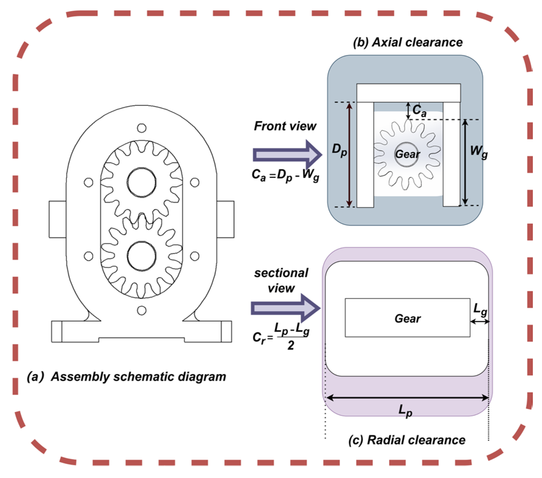
Figure 2.
Part tolerance distribution generated. (a) Pump body bore diameter distribution. (b) Pump body cavity depth distribution. (c) Gear outer diameter distribution. (d) Gear width distribution.
Figure 2.
Part tolerance distribution generated. (a) Pump body bore diameter distribution. (b) Pump body cavity depth distribution. (c) Gear outer diameter distribution. (d) Gear width distribution.
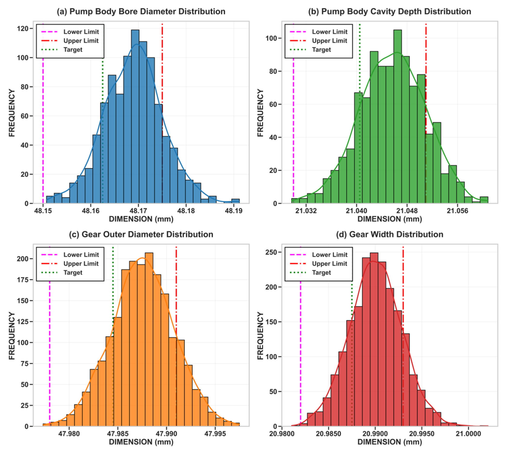
Figure 3.
Assembly clearance distribution generated. (a) Radial clearance distribution (Gear 1). (b) Axial clearance distribution (Gear 1). (c) Radial clearance distribution (Gear 2). (d) Axial clearance distribution (Gear 2).
Figure 3.
Assembly clearance distribution generated. (a) Radial clearance distribution (Gear 1). (b) Axial clearance distribution (Gear 1). (c) Radial clearance distribution (Gear 2). (d) Axial clearance distribution (Gear 2).
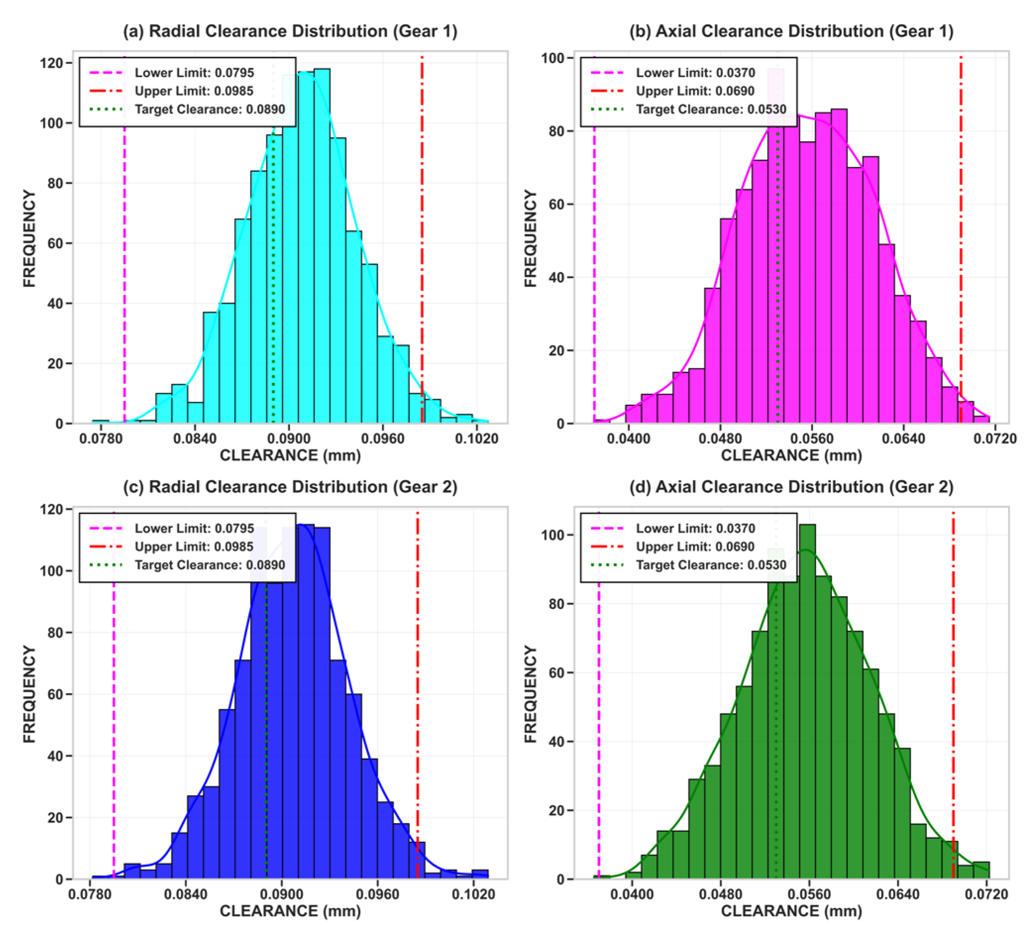
Figure 4.
Taguchi quality loss function.
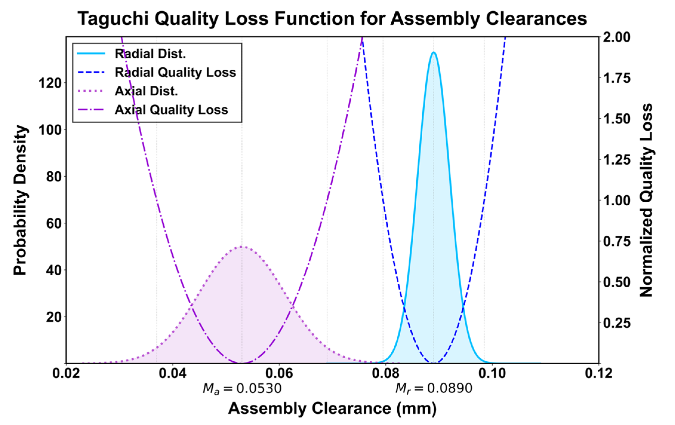
Figure 5.
Ungrouped random matching process.
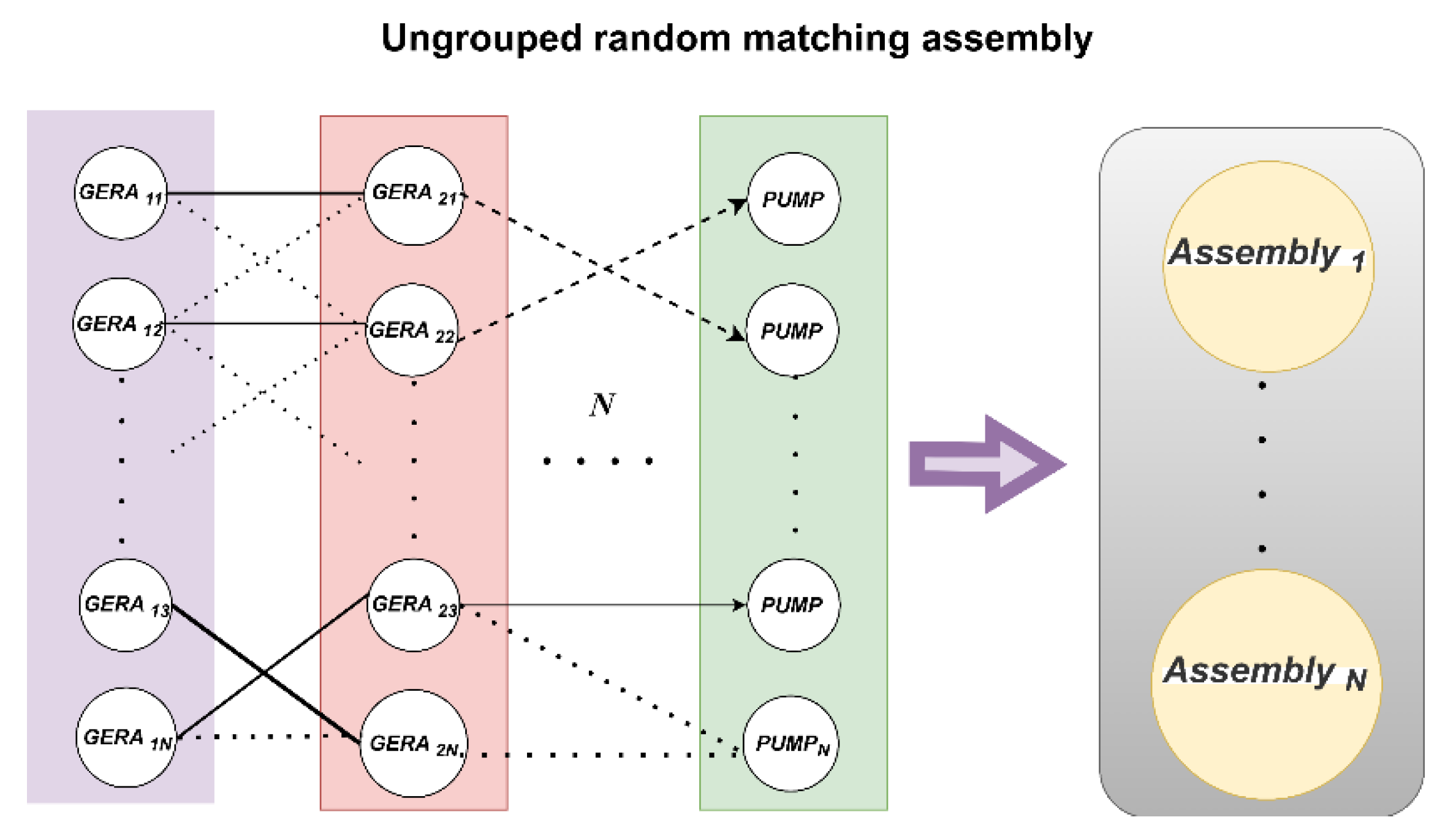
Figure 6.
Cross-operator process.
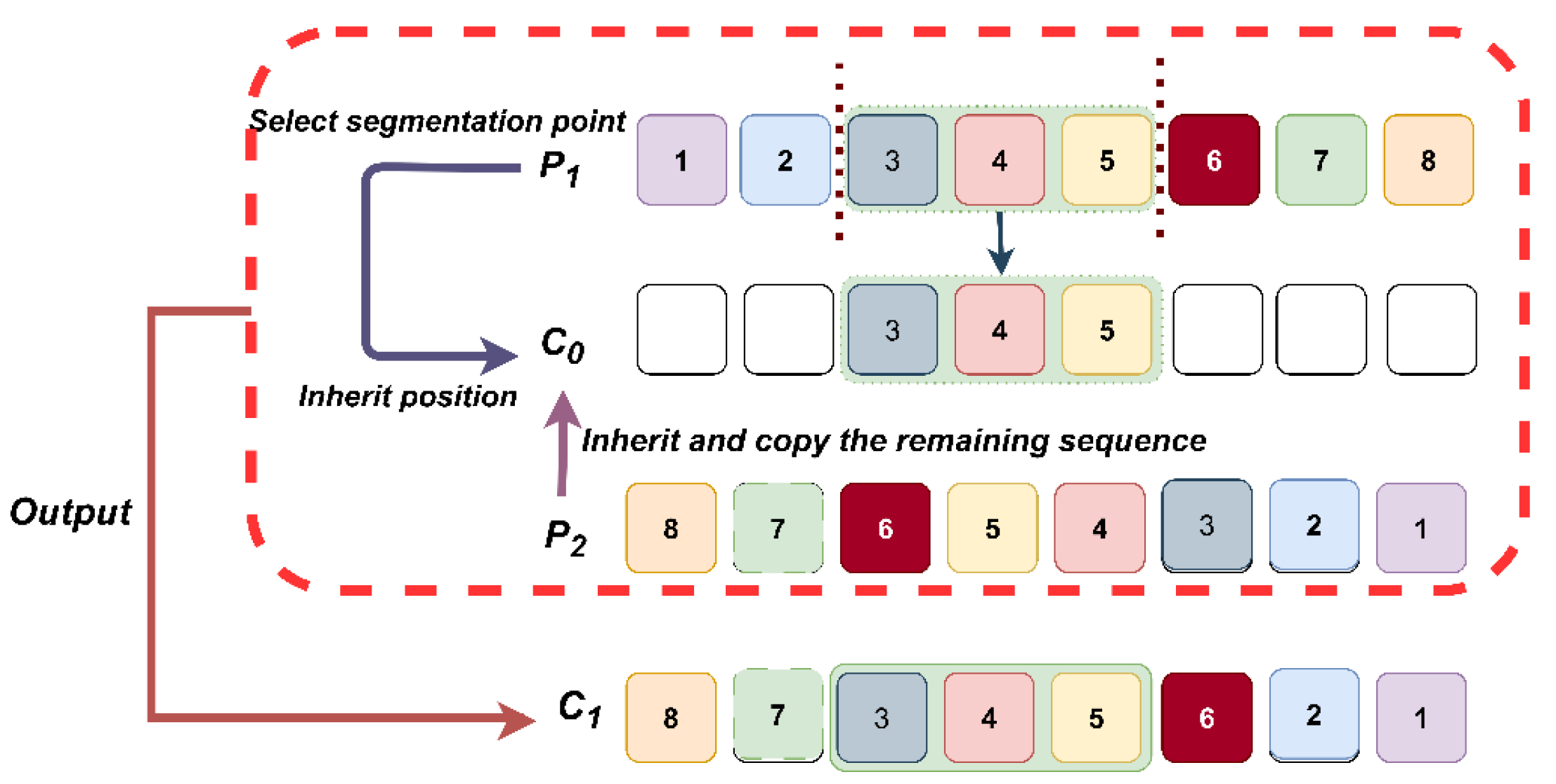
Figure 7.
Inversion mutation process.
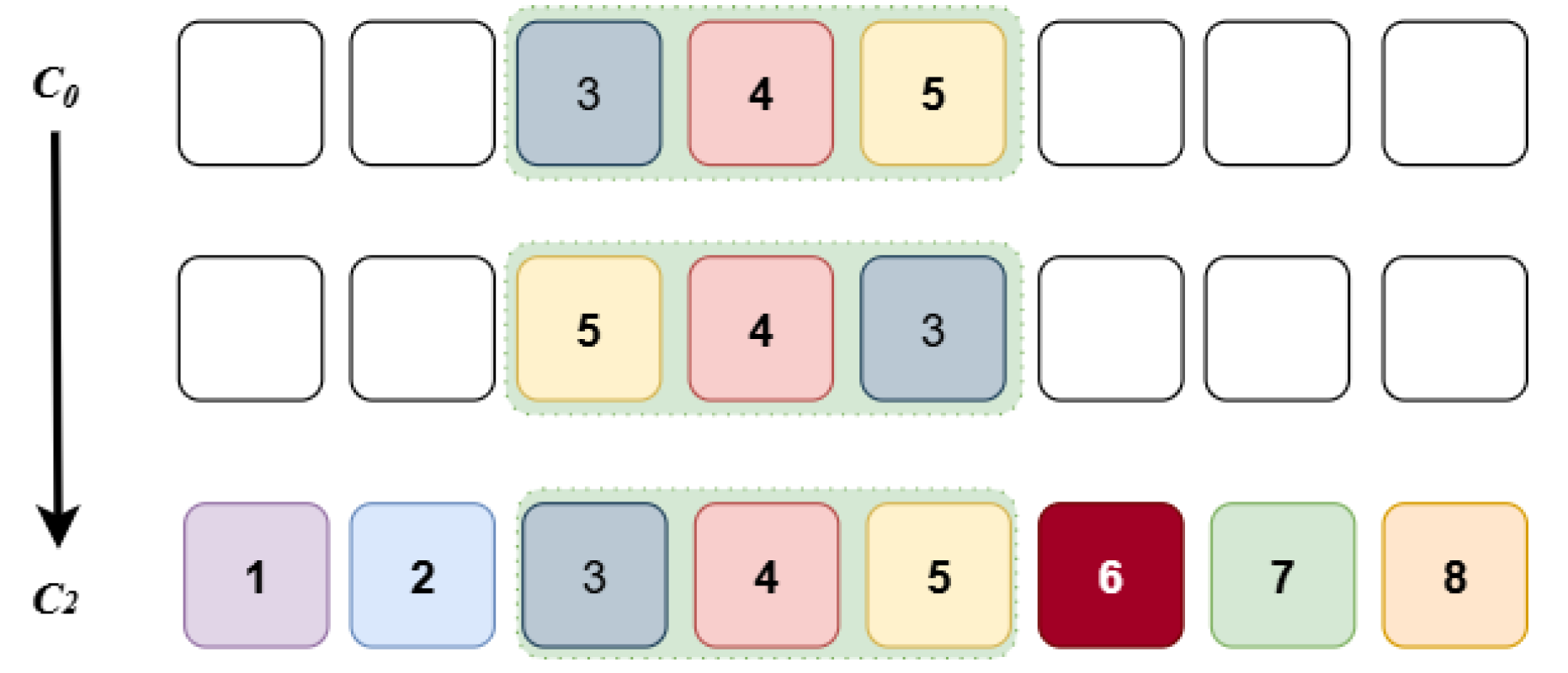
Figure 8.
DE replacement crossover operator.
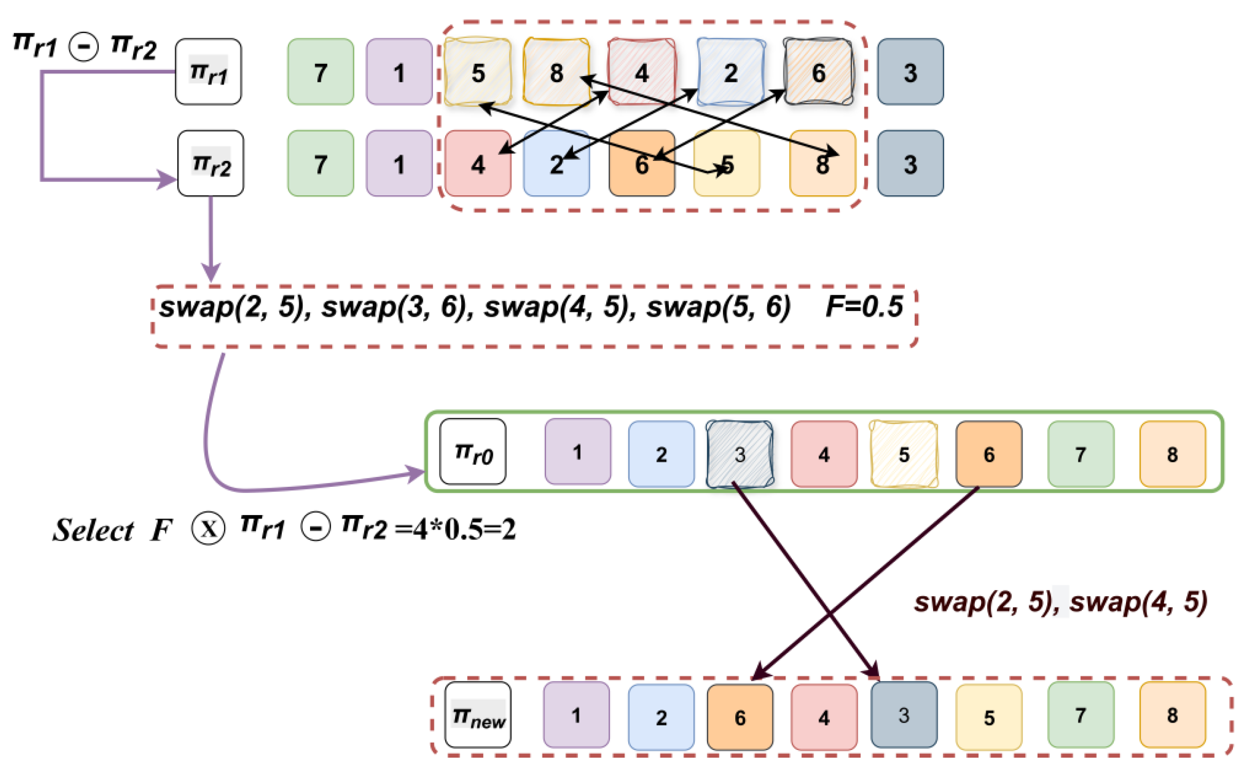
Figure 9.
UCB-MOMA replacement mutation operator.
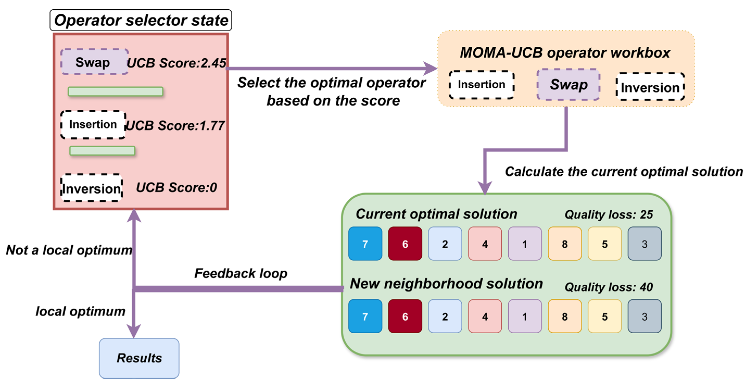
Figure 10.
DG-MA algorithm flowchart.
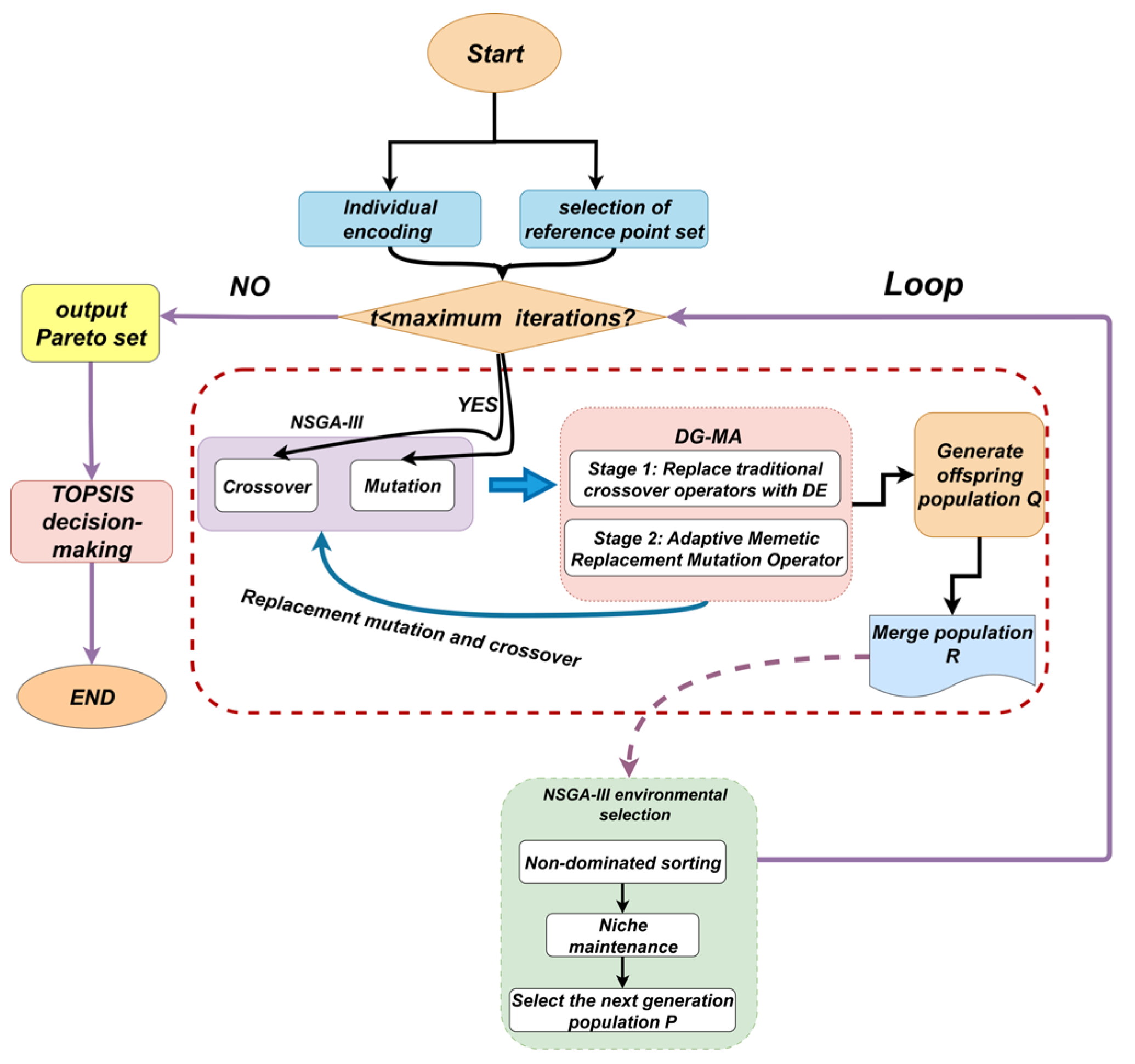
Figure 11.
DG-MA vs traditional selection assembly comparison curve. (a) Quality Performance Analysis: Traditional vs. DG-MA (b) Cumulative Distribution Function.
Figure 11.
DG-MA vs traditional selection assembly comparison curve. (a) Quality Performance Analysis: Traditional vs. DG-MA (b) Cumulative Distribution Function.
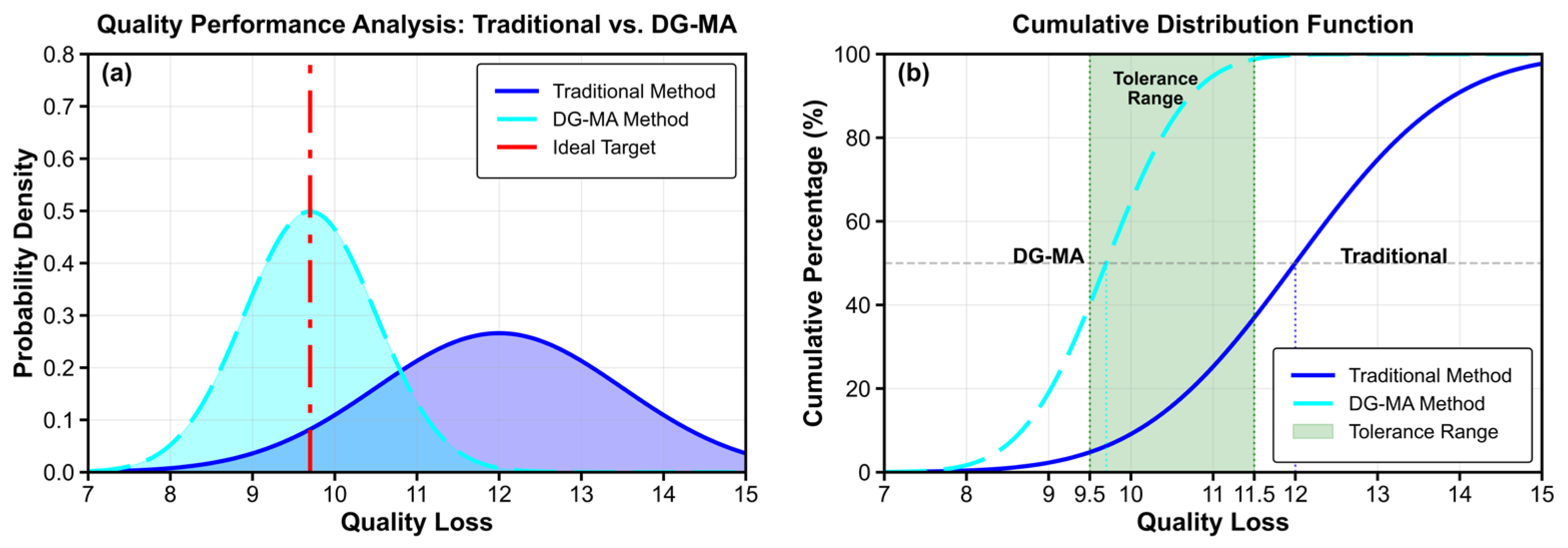
Figure 12.
Performance distribution chart comparing grouped and ungrouped data. (a) Grouped method performance surface. (b) Ungrouped method performance surface.
Figure 12.
Performance distribution chart comparing grouped and ungrouped data. (a) Grouped method performance surface. (b) Ungrouped method performance surface.
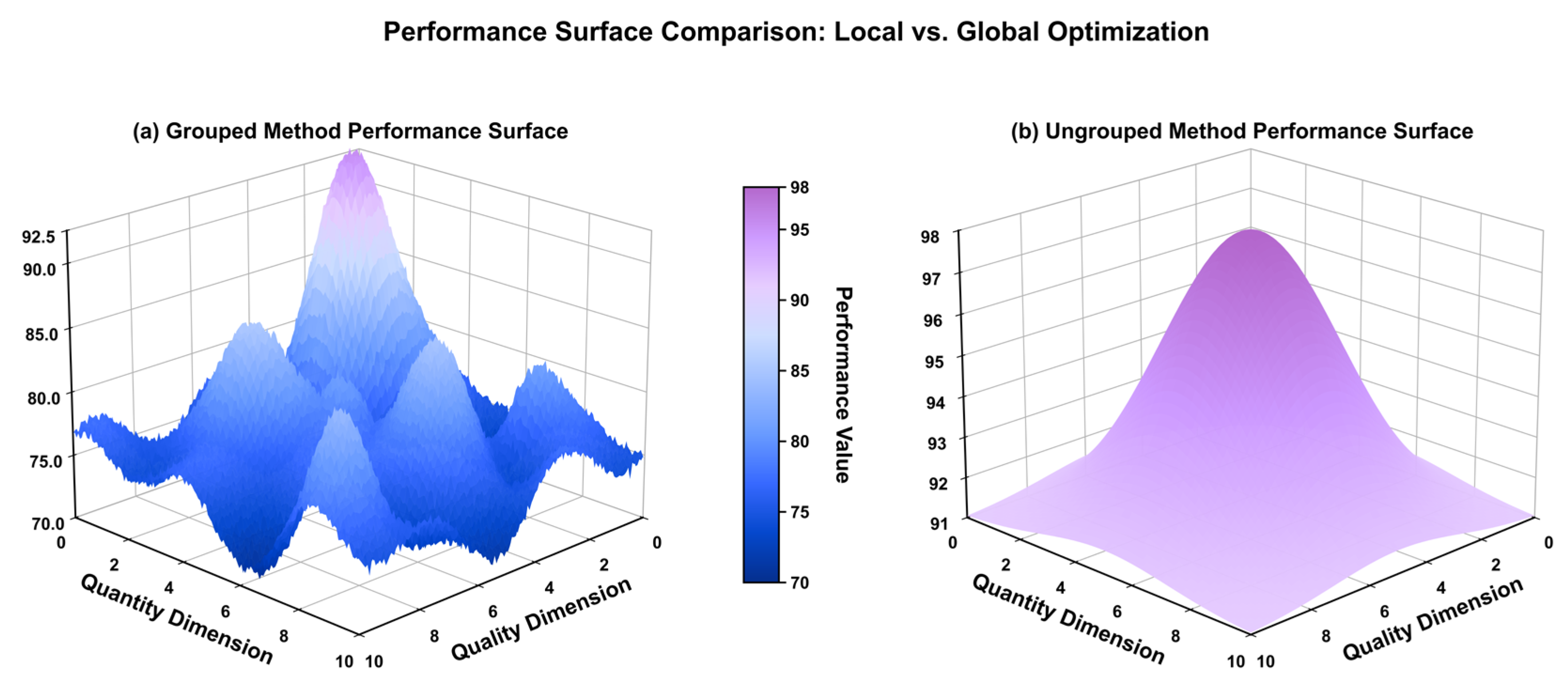
Figure 13.
Algorithm convergence speed curve diagram.
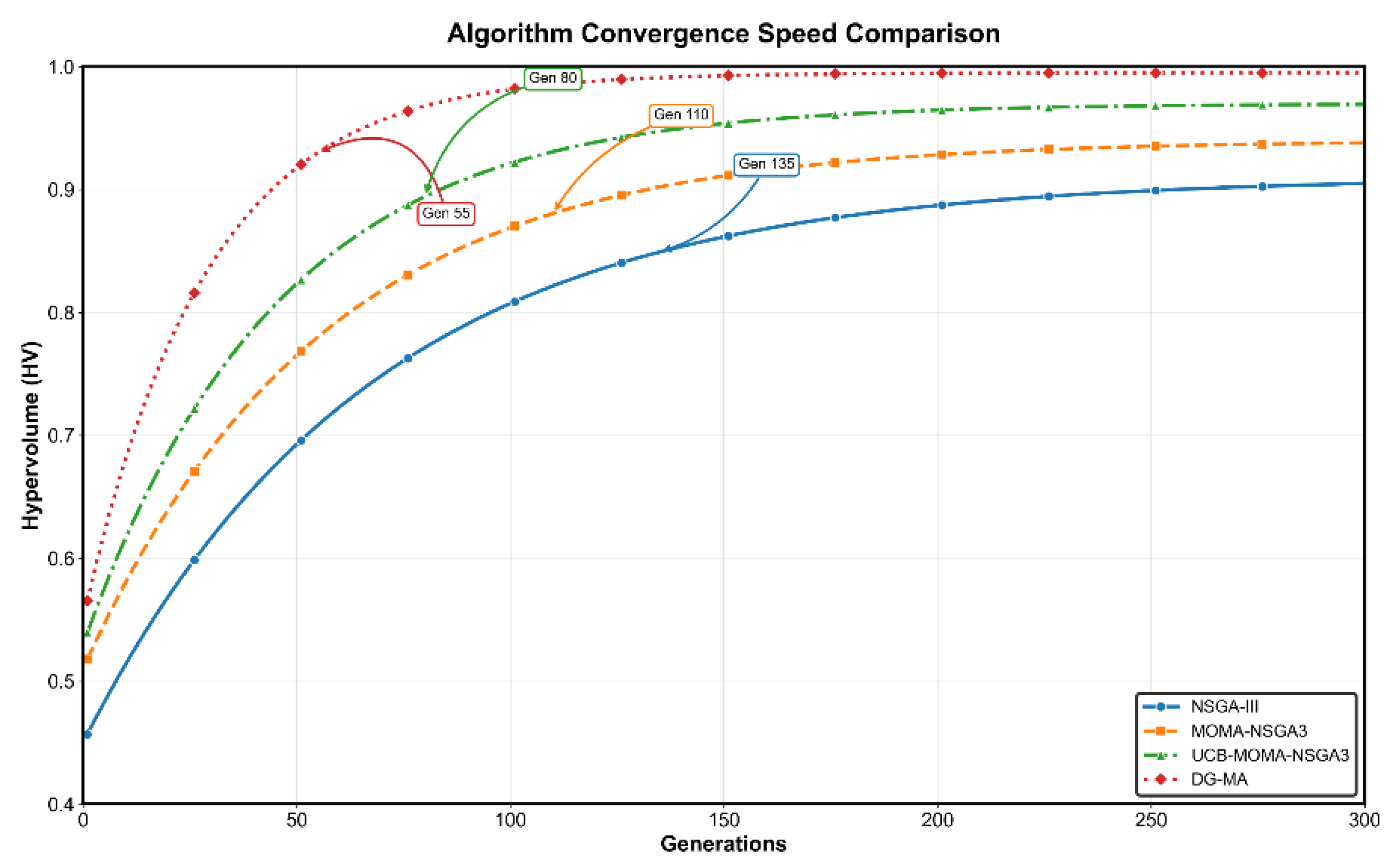
Figure 14.
Comparison box plot. (a) Assembly success rate. (b) Average quality loss. (c) Hypervolume indicator. (d) Convergence speed.
Figure 14.
Comparison box plot. (a) Assembly success rate. (b) Average quality loss. (c) Hypervolume indicator. (d) Convergence speed.
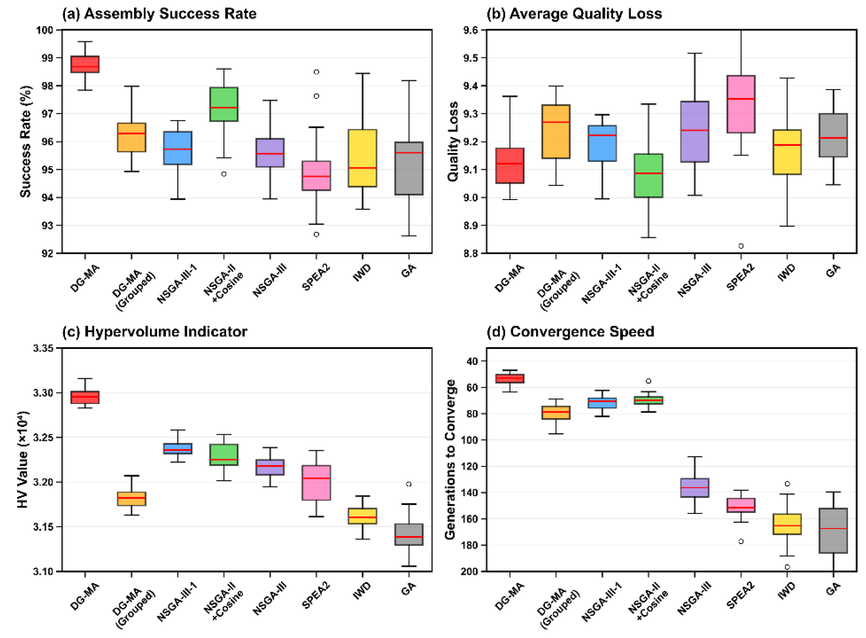
Figure 15.
Convergence curve comparison chart. (a) Convergence performance. (b) Early convergence (0–100 gen).
Figure 15.
Convergence curve comparison chart. (a) Convergence performance. (b) Early convergence (0–100 gen).
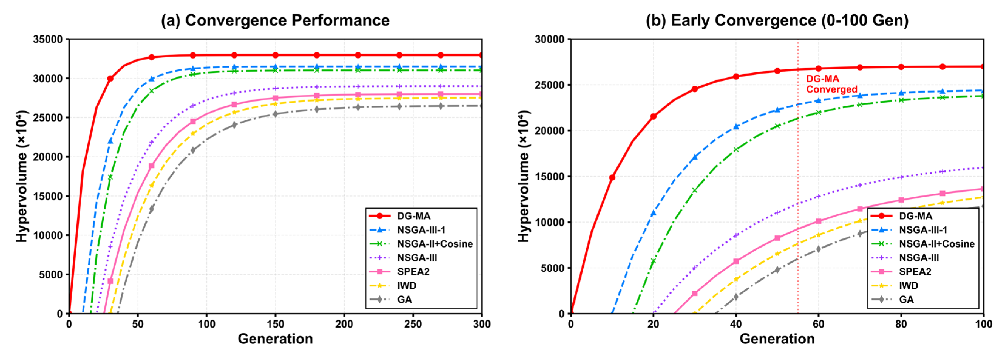
Figure 16.
Comprehensive performance improvement chart.
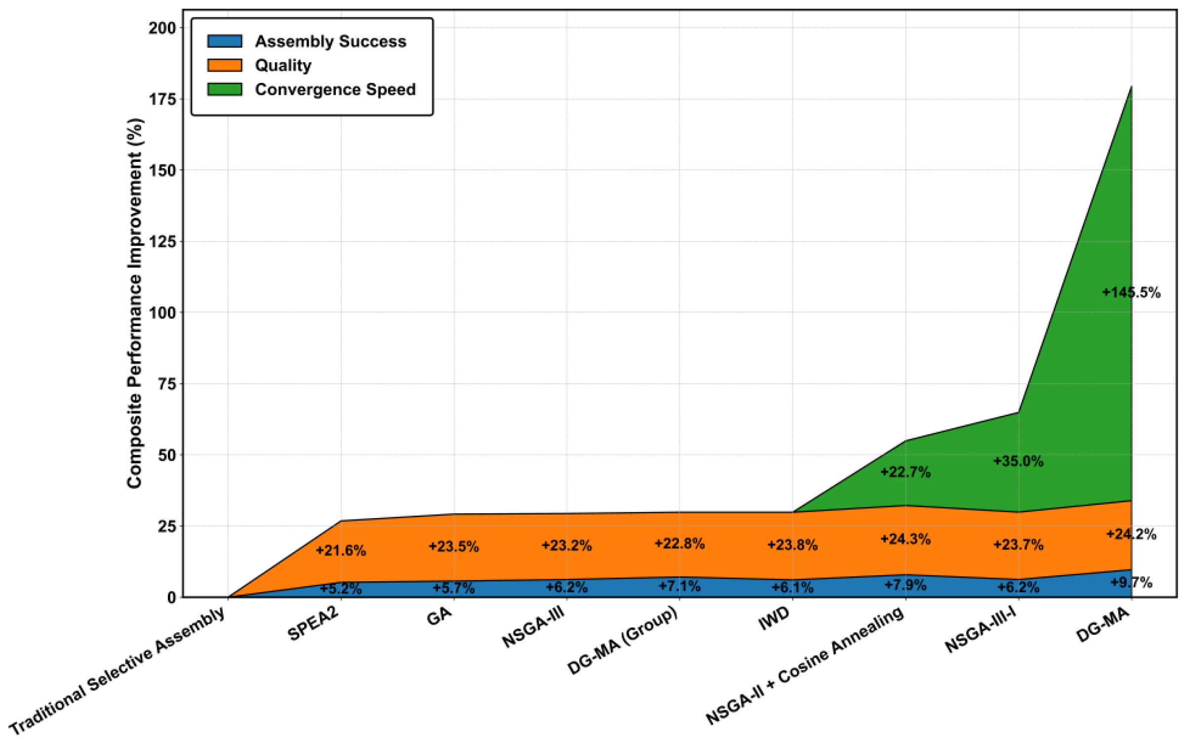
Table 1.
Part dimension data.
| Dimension chain | Ring type | Constituent ring name | Symbol | Nominal dimension (mm) | Tolerance grade (mm) | Upper deviation (mm) | Lower deviation (mm) |
| Radial | Increasing | Pump body bore diameter | 48.15 | H7 | +0.025 | 0 | |
| Radial | Decreasing | Gear outer diameter | 48.00 | g6 | –0.009 | –0.022 | |
| Axial | Increasing | Pump housing cavity depth | 21.03 | H7 | +0.021 | 0 | |
| Axial | Decreasing | Gear width | 21.00 | g6 | –0.007 | –0.018 |
Table 2.
Reference parameters used for Monte Carlo generation of part dimensions.
| Symbol | Tolerance (mm) | Nominal center μ (mm) | Reference scale σ (mm) |
| 0.025 | 48.1625 | 0.00417 | |
| 0.013 | 47.9845 | 0.00217 | |
| 0.021 | 21.0405 | 0.00350 | |
| 0.011 | 20.9875 | 0.00183 |
Table 3.
Detailed results under different optimization strategies.
| Algorithm | Optimization strategy | Successful assemblies (units) | Assembly success rate (%) | Wasted parts (units) | Average quality loss |
| DG-MA | Priority on production | 988 | 98.80 | 36 | 9.09 |
| Priority on quality | 970 | 97.00 | 90 | 8.94 | |
| TOPSIS decision | 988 | 98.80 | 36 | 9.09 | |
| DG-MA (Grouped) | Priority on production | 965 | 96.5 | 103 | 9.27 |
| Priority on quality | 949 | 94.90 | 153 | 10.04 | |
| TOPSIS decision | 965 | 96.5 | 103 | 9.27 | |
| NSGA-III-I [19] | Priority on production | 977 | 97.70 | 59 | 9.15 |
| Priority on quality | 962 | 96.20 | 118 | 9.03 | |
| TOPSIS decision | 977 | 97.70 | 59 | 9.15 | |
| NSGA-II [34] + CA | Priority on production | 975 | 97.50 | 67 | 9.16 |
| Priority on quality | 932 | 93.20 | 204 | 8.76 | |
| TOPSIS decision | 972 | 97.20 | 84 | 9.17 | |
| NSGA-III [28] | Priority on production | 962 | 96.20 | 86 | 9.37 |
| Priority on quality | 949 | 94.90 | 145 | 9.11 | |
| TOPSIS decision | 957 | 95.70 | 119 | 9.22 | |
| SPEA2 [35] | Priority on production | 955 | 95.50 | 135 | 9.55 |
| Priority on quality | 940 | 94.00 | 180 | 9.28 | |
| TOPSIS decision | 948 | 94.80 | 156 | 9.41 | |
| IWD [36] | Priority on production | 956 | 95.60 | 132 | 9.27 |
| Priority on quality | 926 | 92.60 | 222 | 8.95 | |
| TOPSIS decision | 953 | 95.30 | 132 | 9.27 | |
| GA [16] | Priority on production | 952 | 95.20 | 124 | 9.28 |
| Priority on quality TOPSIS decision |
916 952 |
91.60 95.20 |
252 124 |
8.85 9.28 |
|
| Traditional selective assembly | 901 | 90.10 | 153 | 12.00 |
Table 4.
TOPSIS optimal decision comparison table.
| Algorithm | Assembly success rate (%) | Wasted parts (units) | Average quality loss | Best HV value (e+04) | Runs(times) | |
| Algorithm in this paper | DG-MA | 98.80 | 36 | 9.09 | 3.2950 | 25 |
| DG-MA (Grouped) | 96.5 | 103 | 9.27 | 3.1850 | 25 | |
| Academic algorithm | NSGA-III-I [19] | 97.70 | 59 | 9.15 | 3.2315 | 25 |
| NSGA-II [34] + CA | 97.20 | 84 | 9.16 | 3.2287 | 25 | |
| GA [16] | 95.20 | 124 | 9.28 | 3.136 | 25 | |
| NSGA-III [28] | 95.70 | 119 | 9.22 | 3.2172 | 25 | |
| SPEA2 [35] | 94.80 | 156 | 9.41 | 3.1980 | 25 | |
| IWD [36] | 95.30 | 132 | 9.27 | 3.1690 | 25 |
Table 5.
Comparison of comprehensive performance improvement.
| Algorithm | Assembly success ratio (% of successful assemblies) | Assembly quality improvement (%) | Convergence speed improvement (%) |
| DG-MA | 9.70 | 24.20 | 145.5 |
| DG-MA (Grouped) | 7.10 | 22.80 | –32.5 |
| NSGA-III-I | 6.22 | 23.70 | 35.0 |
| NSGA-II + CA | 7.90 | 24.30 | 22.7 |
| NSGA-III | 6.20 | 23.20 | 0.0 |
| GA | 5.70 | 23.50 | –20.6 |
| IWD | 6.10 | 23.80 | –15.6 |
| SPEA2 | 5.22 | 21.60 | –10 |
| Traditional selective assembly | 0.00 | 0.00 | \ |
Table 6.
Assembly performance index comparison.
| Algorithm | Average API | Average runtime |
| DG-MA | 0.98 | 39 min |
| DG-MA (Grouped) | 0.962 | 152 min |
| NSGA-II + CA | 0.958 | 45 min |
| NSGA-III-I | 0.957 | 41 min |
| NSGA-III | 0.949 | 47 min |
Disclaimer/Publisher’s Note: The statements, opinions and data contained in all publications are solely those of the individual author(s) and contributor(s) and not of MDPI and/or the editor(s). MDPI and/or the editor(s) disclaim responsibility for any injury to people or property resulting from any ideas, methods, instructions or products referred to in the content. |
© 2025 by the authors. Licensee MDPI, Basel, Switzerland. This article is an open access article distributed under the terms and conditions of the Creative Commons Attribution (CC BY) license (http://creativecommons.org/licenses/by/4.0/).
Copyright: This open access article is published under a Creative Commons CC BY 4.0 license, which permit the free download, distribution, and reuse, provided that the author and preprint are cited in any reuse.


