
Submitted:
20 January 2025
Posted:
21 January 2025
You are already at the latest version
Abstract
Agricultural equipment market has the characteristics of rapid demand changes and high demand for machine models, etc., so multi variety, small batch, and customized production methods have become the mainstream of agricultural machinery enterprises. Flexible job shop scheduling problem (FJSP) in the context of agricultural machinery and equipment manufacturing is addressed, which involves multiple resources including machines, workers, and automated guided vehicles (AGVs). The aim is to optimize two objectives: makespan and the maximum continuous working hours of all workers. To tackle this complex problem, a Multi-Objective Discrete Grey Wolf Optimization (MODGWO) algorithm is proposed. The MODGWO algorithm integrates a hybrid initialization strategy and a multi-neighborhood local search to effectively balance the exploration and exploitation capabilities. An encoding/decoding method and a method for initializing a mixed population are introduced, which includes operation sequence vector, machine selection vector, worker selection vector, and AGV selection vector. The solution updating mechanism is also designed to be discrete. The performance of the MODGWO algorithm is evaluated through comprehensive experiments using an extended version of the classic Brandimarte test case by randomly adding worker and AGV information. The experimental results demonstrate that MODGWO achieves better performance in identifying high-quality solutions compared to other competitive algorithms, especially for medium and large-scale cases. The proposed algorithm contributes to the research on flexible job shop scheduling under multi-resource constraints, providing a novel solution approach that comprehensively considers both workers and AGVs. The research findings have practical implications for improving production efficiency and balancing multiple objectives in agricultural machinery and equipment manufacturing enterprises.
Keywords:
Agricultural Machinery and Equipment Production
; Flexible Job Shop Scheduling Problem
; Multi-resource Constraints
; Multi-Object Discrete Grey Wolf Optimization algorithm
1. Introduction
As the main manifestation of agricultural productivity, agricultural mechanization equipment is important material foundations for ensuring food security in the context of reducing agricultural labor and achieving agricultural modernization in the context of complex crops. Agricultural mechanization equipment is an important material foundation for the development of modern agriculture. Promoting the development of agricultural mechanization equipment is an objective requirement for improving agricultural labor productivity, land output rate, and resource utilization rate. It is a practical need to support the development of agricultural mechanization, the transformation of agricultural development mode, and the quality and efficiency of agriculture. The production of agricultural mechanization equipment is greatly influenced by market demand, with fast updates and replacements of models and configurations. The demand is highly targeted, and different models need to be selected for different regions, environments, and operational needs[1]. At the same time, the agricultural operating environment varies greatly, and the busy farming hours also vary with climate change, resulting in rapid changes in market demand for various agricultural equipment and diverse demands for machine models. Due to the complexity of the market environment, compared with other mechanical equipment manufacturing industries, agricultural machinery and equipment enterprises have the characteristics of more model selection and unstable market demand cycles in production. Therefore, multi variety, small batch, and customized production methods have become the mainstream of agricultural machinery enterprises, and at present, in order to meet the diversified needs of the market, the production tasks have the characteristics of multi variety and small batch production[2].
In order to meet the diverse demands of the agricultural mechanization equipment production market and achieve flexible production goals of multiple varieties and small batches, manufacturing enterprises can adopt flexible production lines for production. Flexible Job Shop(FJS) is an advanced form of production organization that combines high flexibility and customized production capabilities to adapt to the changing market demands and customer orders in modern manufacturing. It can improve production efficiency, expand production capacity, and meet the assembly needs of multiple types of materials. It also has a certain degree of flexibility, and the products it produces can meet the different needs of customers, and can make corresponding adjustments according to the changes in different customer needs.
The flexible manufacturing shop of agricultural mechanization equipment belongs to the flexible job shop, and its corresponding workshop scheduling problem can be attributed to FJSP. FJSP was firstly introduced in reference[3], accompanied by a polynomial algorithm tailored for addressing small-scale problem instances. Since Brucker and Schlie[3] first delved into FJSP, it has garnered significant attention from numerous scholars. Consequently, many methods have been proposed to tackle this complex issue. The FJSP has been found widespread application in various industrial fields[4-8], including automotive assembly, agricultural machinery equipment production, semiconductor manufacturing and so on.
The extended FJSP which considers the worker-resources-constraint can be seen as a type of dual-resource constrained flexible job shop scheduling problem (DRCFJSP)[9]. Wu et al.[10] addressed a DRCFJSP that incorporated worker learning, with the goal of minimizing the makespan. They devised a hybrid genetic algorithm, integrating variable neighborhood search (VNS), to explore a wide range of potential solutions. Computational tests showed that their algorithm was effective in solving the problem. Kress, Müller, and Nossack[11] studied a DRCFJSP considering setup times and worker skills. They aimed to minimize makespan and tardiness using exact and heuristic methods by splitting the problem into routing and worker assignment subproblems. Gong et al.[12] studied a Double Flexible Job-Shop Scheduling Problem (DFJSP) with a goal to minimize makespan and maximal total worker cost. They proposed a new Hybrid Genetic Algorithm (NHGA) to solve this problem, which outperformed the Non-dominated Sorting Genetic Algorithm II (NSGA-II) in terms of accuracy and efficiency. Vital-Soto et al.[13] tackled the challenge of simultaneously determining machines, worker assignments, and sequencing flexibility in a flexible job-shop setting. Their objective was to minimize makespan, worker workload, and weighted tardiness. They developed a multi-objective optimization model and applied a unique variation of the elitist non-dominated sorting genetic algorithm (NSGA-II) to solve the complex problem they faced.
Collaborative scheduling in workshops involves simultaneously allocating processing machines and AGVs for tasks, aiming to optimize production and transportation resources in a specific workshop environment. Raman et al.[14] first introduced scheduling of AGVs in the flexible job scheduling problem (FJSPT), using a mixed integer programming model to minimize completion time. They treated transportation like operations, with AGVs as machines and travel times as processing times, applying traditional flexible scheduling methods to allocate both machines and AGVs. Yan et al.[15] studied the FJSP problem under limited transportation conditions in a digital twin workshop and designed an improved genetic algorithm to minimize makespan. Hu et al.[16] combined deep reinforcement learning with hybrid AGV scheduling rules for real-time scheduling in flexible workshops. Upon task completion or job arrival, a DQN-based scheduler selects a scheduling rule to allocate the most suitable AGV, aiming to minimize makespan and delay rates. Umar et al.[17] proposed a hybrid multi-objective genetic algorithm to obtain a Pareto solution to the problem of minimizing multiple conflicting objectives, including total makespan, AGV travel time, and delay cost. Similar studies include literature [18, 19].
In summary, many current researches on the dual resource constraints in FJSP mainly focuses on worker and machine constraints, (Automated Guided Vehicle)AGV and machine constraints. However, with the advent of intelligent manufacturing and Industry 4.0 era, the FJSP under multi-resource constraints i.e., Multi-Resource Constrained Flexible Job Shop Scheduling Problem(MRCFJSP) that considers workers, AGVs, and machines together is more in line with the reality of today's workshop production and has become increasingly important and complex. In this paper, a new mathematical model considering machine, worker and AVG in MRCFJSP is established. This model considers operation-sequence-constraint as well as resources constraint such as machine, worker and AVG. To effectively solve this problem, an effective MODGWO algorithm is proposed. The corresponding encoding/decoding method, population initialization strategy, crossover operators and local search technology are designed according to the features of this problem.
2. Materials and Methods
2.1. Problem description
The MRCFJSP considering multiple resource constraints of machines, workers, and AGVs can be described as follows:
There are n jobs J={J1, J2,……,Jn} to be processed, which need to be transported to m machines M={M1, M2,……,Mm} by v AGVs V={V1, V2,……,Vw} for operations by w workers W ={W1, W2,……,Wl}. The machining process of the job is determined, and these processes need to be processed one by one under specific process constraints. The machining process of different jobs is different, and the j-th operation(Oij) of job Ji can be machined on one or more machines. The available set of processing machines for operation Oij is Mij⊆M. The processing time of the same operation on different machines is determined and different. Under the above conditions, with the goal of minimizing the maximum completion time(makespan) and minimizing the workers' continuous working time, allocate a machine Mk∈Mij and a AGV Vv∈V to operation Oij, allocate a worker Ww∈W to machine Mk, and determine the processing sequence of the same operation on the same machine and the transportation sequence of the same operation on the AGV, i.e., decide on the five sub-problems: machine assignment, worker assignment, and AGV assignment, operation sequence and transportation sequence. In addition, the following assumptions need to be satisfied:
(1) Each machine can process at most one operation at a time.
(2) Only one machine must be operated by a worker at a time.
(3) Only one machine and one AVG can be selected for each operation, and they cannot be interrupted during processing.
(4) All the jobs, machines and workers are available at zero time. All the jobs and AGVs are located in loading/unloading(LU) area at zero time.
(5) The processing operations for the same job shall meet the constraints of the operation sequence.
(6) Disregarding the transfer time of workers between machines, a worker can only operate one machine at a time.
(7) Machines and AVGs failures are not considered and the AVGs is sufficiently charged, and the loading and unloading time of the material on the machine is not considered.
(8) An AVG can only load one job at a time.
(9) After the current transportation task is completed, the AGV will not return to the loading and unloading area, but will go to the machine where the next transportation task is to be performed.
(10) Each machine has a buffer zone that can be used to park AGVs and store operations with sufficient buffer capacity.
Figure 1 illustrates a specific scenario. AGV, workers, and machines are regarded as three different resources in the production workshop. AGV is responsible for transporting raw materials from the loading area to various machines, thus establishing an important logistics chain. Starting from the loading area, the AGV picks up tasks one by one and transports them to the designated machine, as shown in loaded AGVs in Figure 1. Then, the machine is operated by a worker to start the processing task. Alternatively, the AGV can run empty to a certain machine and transport the semi-finished products to the machine to be processed in the next process, such as unloaded AVGs. Workers operate machines when they have processing tasks assigned, and they can take a break in the resting area when not assigned to any tasks. This continuous cycle process ensures efficient workflow and sustained productivity in the workshop.
2.2. Mathematical model
The notations required for the mathematical model are listed in Table 1.
Based on the above problem definition, constraints, assumptions and notations, the mathematical model of MRCFJSP is established as follows.
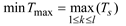
This paper considers two optimization objectives. Eq. (1) represents minimizing the maximum completion time of last job(makespan). The second objective is to minimize the maximum continuous working hours of all workers, which is shown in Eq. (2).
Subject to:
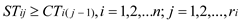
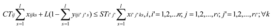

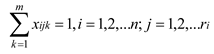
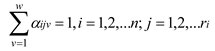


where Eq. (3) indicates that the completion time of each job is after the start time. Eq. (4) represents the processing sequence constraint of a job. Eq. (5) to Eq. (7) represent the processing time constraint, which can guarantee that each operation cannot start until the assigned machine, worker and AVG are ready. Each machine can only process at most one operation and can only be operated by one worker at a time are shown in Eq. (8) and Eq. (9), respectively. Eq. (10) to Eq. (12) can ensure that each operation can be assigned to only one machine, one worker and one AVG respectively. Eq. (13) to Eq. (18) indicate that all decision variables are 0-1 variables.
2.3. Grey Wolf Optimization algorithm
The Grey Wolf Optimization(GWO)[20] algorithm was initially proposed by Australian scholars Seyedali Mirjalili et al. in 2014 for continuous real parameter optimization problems, and has been improved to handle some practical engineering problems[21-24]. As shown in Figure 2, the grey wolf pack has a very strict social hierarchy similar to the pyramid. The first three hierarchical categories are Alpha(α), Beta(β), and Delta(δ) as the best solutions to lead the rest of the wolves named Omega(ω) wolves toward promising areas in order to find the global solution.
A wolf(i) evaluates its proximity to the three best solutions based on Eq. (19)–(22) and subsequently updates its position using Eq. (23).
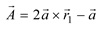

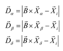
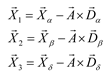
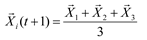
Where i, α, β, and δ, indicate the position vectors of wolf i, α, β and δ; i(t+1) is the location of the wolf i in the next iteration; 1and 2are random vectors in [0,1]; and are two coefficient vectors where the vector is linearly decrease from 2 to 0 over the course of iterations and can be calculated by Eq. (24).
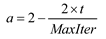
Where where t is the present number of iteration and MaxIter represents the max number of iteration.
2.4. Multi-Object Discrete Grey Wolf Optimization algorithm for MRCFJSP
For continuous optimization problems, the grey wolf individual position can be updated by Eq.(19)-(23), however, MRCFJSP is a discrete problem and cannot be directly solved using the above formulas. This paper proposed a MODGWO algorithm for MRCFJSP based on the characteristics of the problem and combined with cross operation in genetic algorithm. First, an encoding/decoding method is introduced, followed by a method for initializing a mixed population. Then the Discrete Grey Wolf iteration operators are presented for global search. Finally, an effective VNS with four neighborhood structures is introduced to improve the local search ability.
To clarify the proposed algorithm, an 3×3×2×2 instance involving three jobs, three machines, two workers and two AVGs is provided in Table 2 and Table 3. Table 2 outlines the fundamental processing durations, while Table 3 displays the information of machines that workers can operate. The symbol ‘–’ signifies that a machine is incompatible with a particular operation or a worker is unable to operate a specific machine. In addition, by default, each AGV can transport all jobs.
2.4.1. Four-vector encoding
The efficiency of encoding and decoding techniques has a substantial influence on algorithm performance. Utilizing effective encoding and decoding methods can facilitate algorithm operations and enhance computational performance. The MRCFJSP needs to solve four sub-problems: operation scheduling, machine selection, worker selection, and AVG selection. Therefor in this subsection, we introduce an encoding scheme where each individual comprises four distinct vectors: the Operation Sequence(OS) vector, which denotes the order of operation execution; the Machine Selection(MS) vector, which specifies the assignment of machines; the Worker Selection(WS) vector, which outlines the allocation of workers; and the AVG Selection(AS) vector, which indicts the assignment of AVGs. Collectively, these four vectors constitute a viable solution for the MRCFJSP. In the four-layer coding method, we borrowed the idea of MOSO coding method proposed by Ho et al[25]. Figure 3 shows the four vector representation approach of the examples in Table 1 and Table2, where green indicates job 1, yellow indicates job 2 and blue indicates job 3.
(1) Operation sequence vector
An OS vector consists of an array of integers where the number of array elements equals the total number of operations in all jobs. Each operation is denoted by its corresponding job index. Specifically, the jth occurrence of index i signifies the jth operation within job i, and the count of index i repetitions is equivalent to the total number of operations in job i.
For example {3, 2, 1, 2, 3, 1, 1} is a legal vector or the aforementioned instance shown in Table 2 and Figure 3(a). The sequence of operational decoding for this OS vector is O31→O21→O11→O22→O32→O12→O13.
(2) Machine selection vector
A MS vector consists of an array of integers, the length of which equals to the length of OS vector and each element indicates an available machine for the corresponding operation.
A MS vector {1, 3, 2, 1, 3, 1, 2} means that for the operation set {O11, O12, O13, O21, O22, O31, O32}, the machine selection indicated by the MS vector is {M1, M3, M2, M1, M3, M1, M2} correspondingly shown in Figure 3(b).
(3) Worker selection vector and AGV selection vector
The WS vector and AS vector are encoded in a similar way to MS vector. As shown in Figure 3(c), the first number 1 in the WS vector represents the O11 is processed by worker W1 on machine M1. The WS vector {1, 2, 2, 1, 1, 1, 2} indicates that the operations {O11, O12, O13, O21, O22, O31, O32} are processed by workers {W1, W2, W2, W1, W1, W1, W2} on machines {M1, M3, M2, M1, M3, M1, M2} respectively. Similarly, the AS vector {1, 1, 2, 1, 2, 2, 1} shown in Figure 3(d) represents that the operations{O11, O12, O13, O21, O22, O31, O32} are transported by AGVs{V1, V1, V2, V1, V2, V2, V1} respectively.
2.4.2. Decoding
There are mainly four approaches to decode a solution represented by the four-vector encoding scheme: non-delay, semi-active, active and hybrid schedules. In this paper, the active schedule is utilized to decode all the solutions. The decoding procedure is as follows: (1) Pick out the operations from the OS vector one by one from left to right, assign the corresponding machine, worker and AGV to the current job in sequence. (2) Determine the starting time of the current job from the earliest available start time of the corresponding machine, worker, and AVG, until the last job is processed. (3) Arrange the operations at their earliest feasible time. (4) Calculate the maximum completion time and maximum worker duration, which are the values of the two objective functions.
2.4.3. Population initialization
The standard of initial solutions significantly influences how well an algorithm performs in producing high-quality solutions. Recognizing the significant impact of population initialization on the algorithm's performance, we propose several adaptive strategies aimed at enhancing the quality of the initial population. To achieve a balance between the quality and diversity of initial solutions within the search space, we utilize a hybrid approach that combines random generation with strategic selection to form the initial population. Since the problem in this paper is divided into four sub-problems, operation sequencing, machine selection, worker selection and AVG selection, the population initialization is also carried out in four stages. Firstly, the initialization of OS vectors employs a hybrid approach[26] according to the following three rules:
(1) Most work remaining rule[27]: the job that has the maximum total processing time remaining is prioritized for execution first.
(2) Most number of operations remaining rule[26]: the job that has the most remaining operations is processed first.
(3) Random rule: operation sequencing is randomly generated.
The aforementioned three rules are utilized in the generation of OS vectors, and their respective proportions are 30%, 30%, and 40%. The initialization of MS vectors is initialized employing the following three rules:
(1) Global minimum processing time rule[28]: select the machine with the shortest processing time for the current operation.
(2) Workload considered rule[29]: Assign machines according to the machine workload.
(3) Random rule: Randomly assign machines.
The machine selection of the population is sequentially generated using the first and second rule in the proportion of 30% and the remaining 40% by random rule. The initialization process of the WS vectors and the AS vectors is similar to that of MS vectors, the only difference is that only workers and AVGs load, as well as random allocation, are used, with respective proportions of 50% and 50%.
2.4.4. Solution updating mechanism
Since the basic GWO cannot be directly applied to the discrete scheduling problem, this paper designs a discrete version of the solution updating mechanism for the machine selection, AGV selection and operation sequence. The grey wolf individual crosses with wolf α, wolf β, and wolfδaccording to a certain probability, and thus obtains a new individual, as shown in Eq. (25).
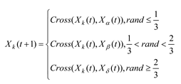
where Xk is the position vector of grey wolf t, Xα, Xβ, and Xδ are the position vectors of grey wolf α, β, andδ, respectively, rand is a random number that follows a uniform distribution between 0 and 1. Cross is the crossover operator, and the specific crossover method for each vector is described in detail below.
In basic GWO, new individuals are generated based on the information of the three individuals α, β, andδ that are currently serving as the decision level individuals. To determine α, β, andδ individuals within a population, this paper adopts a method based on non dominated level and crowding distance to obtain decision level individuals, that is, sorting individuals according to their non dominated level and crowding distance in the population, and the top three individuals have the opportunity to become decision level individuals. For any two individuals, the individual with the lower level ranks is selected first, if two individuals have the same level, compare their crowding distance, and the individual with the larger crowding distance ranks first.
Meanwhile, we integrate the ideas of Jaya algorithm into the proposed MODGWO. The Jaya algorithm is a novel population-based metaheuristic recently proposed by Rao[30], which is based on the principle of continuous improvement, and improves the quality of the solution by moving the individuals closer to the best solution while moving away from the worst solution. Jaya algorithm iteratively evolves through Eq. (26). to obtain new solutions.
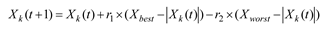
where Xk(t+1) is the updated solution corresponding to the initial solution Xk(t). Xbest and Xworst represent the best and worst solutions of the current population, respectively. r1 and r2 are uniformly distributed. In the improved MODGWO, one of Xα, Xβ, and Xδ is randomly chosen as Xbestusing Eq. (25), while the worst individual Xworst is selected from the last rank having the minimum crowding distance value. The detailed procedures for operation sequencing, machine selection, worker selection and AVG selection are summarized below.
(1) Operation sequencing
This paper draws on the method in literature [31] to delete sequences in the current solution that are identical to the worst solution and replace them with the best solution. The specific steps are as follows:
Step 1. Identify the worst individual (Xworst) and choose one form Xα, Xβ, and Xδrandomly as Xbest (assuming that Xβ is selected) from the population.
Step2. Identify similar assignments of operations in the individual Xi and Xworst.
Step 3. Eliminate similar assignments from Xi and transfer the remaining assignments to a new solution Xinew.
Step 4. Beginning from the initial assignment of Xβ, eliminate the assignments corresponding to the remaining assignments of individual Xinew.
Step 5. Beginning from the initial assignment of Xβ, transfer the remaining assignments of Xβ in the vacant elements of individual Xinew in the corresponding order.
Figure 4 illustrates the operation sequencing vector updating mechanism.
(2) Machine selection and AGV selection
The solution updating mechanism for the machine selection and AVG selection is the same and similar to that of operation sequencing.Only the detailed steps for updating machine selection are as follows:
Step 1. Identify the best individual Xbest(Assuming it is Xα) and worst individual Xworst from the population.
Step 2. Identify similar assignments of machines assigned to the same machines in the individuals Xi and Xworst.
Step 3. Eliminate similar assignments from the individual Xiand transfer the remaining assignments to a new solution Xinew.
Step 4. Transfer the corresponding machine assignments of Xα to the vacant elements of individual Xinew.
Figure 5 illustrates the machine selection vector updating mechanism.
(3) Worker selection
The updating mechanism of worker selection is the same as the previous steps of machine selection and AVG selection, eliminating elements from the current individual that correspond to the position of the worst solution, and filling the eliminated elements with elements corresponding to the position of the best solution. Finally, it is necessary to conduct feasible checks on new individuals. Check for the feasibility of each assignment of Xinew based on the capable worker set of the corresponding machine in the updated machine selection vector. If infeasible randomly allocate an integer value within the capable worker set range.
2.4.5. Local search
To enhance the local search capability, variable neighborhood search operations are performed on the OS, MS, WS and AS of the optimal individuals after each iteration, respectively. Variable neighborhood search (VNS) can expand the search space of the algorithm by changing the domain structure based on problem features, avoiding the algorithm from falling into the local optimal solution. Firstly, the initial solution that requires neighborhood search is given. Secondly, the neighborhood structure is used for neighborhood search to obtain the neighborhood structure solution. If the target value of the neighborhood solution is better than the current solution, the current solution is updated and the weights are updated. The search returns to the first neighborhood structure and starts again until a better solution cannot be found. Then, the next neighborhood structure is reached for search until all neighborhood structures have been searched. Based on the characteristics of the MRCFJSP, the following 4 domain structures are constructed:
(1) VNS1(Insert, for OS vectors)Within the length range of OS vector, randomly generate two positions r1 and r2 (r1<r2), insert the element corresponding to r2 into position r1, and move the elements after position r1 backwards in sequence. For the OS vector in Figure 3, the two generated random numbers r1 and r2 are 2 and 5, respectively. The solution process of VNS1 is shown in Figure 6.
(2) VNS2(Choose the minimum processing time,for MS vectors)Randomly generate r ϵ [1, N] random numbers, where N is the total number of operations, and randomly select r positions from the MS vector. For each selected position corresponding to a operation, select the machine with the shortest processing time from its corresponding optional machine set for replacement. After replacement, check whether the workers corresponding to r positions in WS can operate the newly selected equipment. If it is not feasible, randomly select a worker from the operable worker set of the new equipment. For the solution generated in Table 2.1, MS is 1122312, and r=3 is randomly generated. Three positions are randomly selected, such as positions 2, 3, and 7. The solution process of VNS2 is shown in Figure 7.
(3) VNS3(Flip, for WS vectors)Within the length range of WS vector, randomly generate a position r1. In MS vector, position r1 should correspond to more than one available processing worker for the processing equipment, and then select a new worker from the set of available workers for equipment replacement.The solution process of VNS3 is shown in Figure 8.
(4) VNS4(swap, for AS vectors)Within the length of the AS vector, two randomly generated positions r1 and r2 (r1 ≠ r2) are exchanged for the elements at the r1 and r2 positions. The solution process of VNS4 is shown in Figure 9.
3. Results
The proposed approach is coded in Python 3.9 on an Intel i7 processor with a speed of 2.6 GHz on a Windows 11 operating system with 16 GB RAM.
3.1. Performance metrics
To assess the efficacy of the Pareto front derived from various perspectives, we employ two metrics: IGD[32], and the Hypervolume[33]. The aforementioned metrics encompass various facets concerning the quality of non-dominated solutions, particularly focusing on those derived from Pareto-based approaches. The detailed explanation of these two metrics is summarized below.
(1) Inverse Generational Distance (IGD): Measure the average distance from a predefined set of uniformly spaced points along the true or ideal Pareto Front (denoted as PF*) to the nearest solution in the obtained PF. Essentially, IGD assesses how well the obtained solutions approximate the true Pareto Front by calculating these distances and averaging them.
The formula for the IGD is typically expressed as follows:
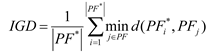
where:
- |PF*| is the number of uniformly spaced points along the true Pareto Front.
- PF*i represents the i-th point in PF*.
- PF is the set of obtained solutions (Pareto Front).
- PFj represents the j-th solution in PF.
- d(PF*i , PFj)is the Euclidean distance between point PF*iand the closest solution PFjin PF.
A lower IGD value indicates that the obtained PF is closer to the true Pareto Front, suggesting better performance of the optimization algorithm in identifying high-quality solutions. Since the actual PF* of MRCFJSP in this paper is unknown, the non dominated solutions from multiple runs of all algorithms are first integrated into a hybrid solution set, and then the non dominated solutions in the hybrid solution set are used as PF*.
(2) Hypervolume(HV): HV is the volume of a hyper polyhedron enclosed by non dominated solutions and reference points in the search space, calculated as follows:
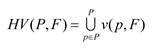
where P represents the Pareto Front approximate non dominated solution set obtained by the algorithm, F represents the reference points of the solution set, v is the volume of a hypercube enclosed by the p-th solution and the reference points. The target vectors corresponding to all Pareto solutions are normalized and the reference point for calculating HV is set to (1, 1).
3.2. Test instances generation
This paper extends the classic Brandimarte test case [27] in the flexible job shop scheduling problem by randomly adding worker and AVG information for solving the MRCFJSP. The number of workers in each workshop is calculated by multiplying the number of machine in the workshop by 0.6 and rounding up, and the probability that a worker can operate a certain machine is 0.5. For each test case, the ratio of the number of AGVs to the number of machines is considered to be 1:1, 1:2, and 1:3, respectively. Taking MK01 as an example, this example has 10 jobs and 6 machines. In the generated new example, the number of workers is 4, and the number of AVGs is 6, 3, and 2, respectively. The names of the extended examples are MK01_4_6, MK01_4_3, and MK01_4_2. In this way, 45 instances for MRCFJSP are used to test in this study, and Table 4 shows the relevant information, where n represents the number of jobs and m represents the number of machines..
3.3. Effectiveness verification for a hybrid initialization method
To verify the effectiveness of the hybrid initialization method and local search proposed procedure in this paper, it is compared with the random initialization method and method without local search, the comparison algorithms are as follows:
(1) MODGWO represents the method proposed in this paper.
(2) RI(Random Initialization) indicates that MODGWO uses a random initialization method to obtain the initial solution.
(3) WLS(Without Local Search) indicates that MODGWO does not use a local search procedure, but only a single tracking mode for searching.
Each method was independently run 20 times based on the expanded 45 test cases. The average values of IGD and HV were calculated based on the non dominated solution sets obtained by the three methods and calculated results are shown in Table 5. The results from Table 5 are shown as box plots in Figure 10.
The experimental results show that MODGWO can obtain better initial populations compared to RI which benefited from the effective diversity strategy introduced in their initialization. Compared with RI, MODGWO achieved a total of 40 minimum values on IGD and 38 maximum values on HV, indicating that the diversified initialization method proposed in this paper can obtain better quality and more Pareto solutions. And the 5 best IGD values obtained from RI method are all concentrated in smaller scale cases, indicating that for medium and large-scale cases, a diverse population initialization method is needed to obtain better solutions.
To assess the effectiveness of the proposed local search procedure, we compare WLS to MODGWO and RI for all problem instances. From Table 5 and Figure 10, it is seen that MODGWO and RI outperforms WLS for all data sets for IGD and HV metrics. The poor performance of WLS concerning the IGD and HV metrics can be attributed to the algorithm’s the absence of the local search procedure. On the whole, the introduced local search procedure plays a crucial role within the proposed methodology and has a substantial impact on enhancing the convergence performance of MODGWO. This indicates that the local search mechanism is integral to the overall effectiveness and efficiency of the MODGWO algorithm in finding optimal or near-optimal solutions to MRCFJSP.
3.4. Comparison with other algorithms
There have been many studies on flexible job shop scheduling under dual resource constraints for workers alone [34-36], as well as flexible job shop scheduling under AGV constraints alone [37-39]. However, there is a lack of research on flexible job shop scheduling under multi-resource constraints that comprehensively consider both workers and AGVs. Therefore, this paper chooses MOPSO proposed by Zhang et al. [40], MOJAYA proposed by Rylan H et al. [41], and NSGA II which is commonly used to solve multi-objective flexible job shop scheduling problems as comparative algorithms. These three algorithms have been often used to solve FJSP under resource constraints, which are most similar to the problem studied in this paper.
The experimental results for the two performance indicators have been organized in Table 6. Regarding the IGD metric detailed in Table 6, MODGWO demonstrates a notable superiority over its rival algorithms across all datasets. In 45 cases, MODGWO achieves 39 minimum values, while MOJAYA achieves 6 minimum values. It indicates that MODGWO exhibits superior exploration and exploitation capabilities. In comparison to MOPSO and NSGA-II, MOJAYA exhibits superior performance. Additionally, NSGA-II displays a competitive performance that is comparable to MOPSO. As for the HV metric, a similar trend is observed in Table 6, MODGWO demonstrates a significantly better performance as compared to other algorithms. In 45 cases, the MODGWO achieves 38 optimal values, and the MOJAYA achieves 7 optimal values. MOJAYA offers a better performance in terms of obtained metric values and the number of significantly better instances.
This indicates that both MODGWO and MOJAYA can obtain good solutions when solving MRCFJSP, with MODGWO yielding better results than MOJAYA. From Eq. (26), it can be seen that the Jaya algorithm drives the entire population to converge quickly to the global optimal solution through the optimal solution at each iteration, while from Eq. (25), the GWO algorithm drives the population to converge to the global optimal solution through the first three optimal solutions. This ensures the diversity of solutions and avoids the population from falling into local optimal solutions earlier. Therefore, MODGWO proposed in this paper combines the advantages of GWO algorithm and Jaya algorithm, which can effectively solve MRCFJSP.
To gain a deeper understanding of MODGWO's performance, especially regarding its convergence and diversity in tackling optimization challenges of varying scales, we compare its effectiveness based on small, medium, and large problem sizes. Benchmark instances are classified based on their jobs, machines, and operations. This detailed classification can more thoroughly evaluate the capabilities of the algorithms. The performance of the compared algorithms in terms of IGD, and HV metrics for selected instances are shown in Figure 11, Figure 12 and Figure 13.
Figure 11 depicts the comparative performance of the algorithms on smaller-scale instances. Specifically, as observed in Figure 11(a), MODGWO demonstrates superior performance in terms of the IGD metric for most instances, outperforming the other algorithms. Except for slightly lower performance than MOJAYA on MK_02_4_6 and MK05_3_2 instances, MODGWO achieves the best results on all other instances. Figure 11(b) shows the performance of the compared algorithms in terms of the HV metric. A similar trend is observed, as the IGD metric, with MODGWO performing poorly on MK02_4_6 and MK04_5_8 instances. MOJAYA surpasses NSGA-II and MOPSO in most instances while maintaining a competitive edge against MODGWO. Both NSGA-II and MOPSO exhibit comparable performance, suggesting a similar level of diversity and convergence in their respective Pareto solutions.
The comparison of medium scale instances is shown in Figure 12. As seen in Figure 12(a), in terms of IGD metrics, MODGWO performs well as compared to other algorithms for all instances except for MK06_6_5 and MK07_3_5 instances. MOJAYA is superior to NSGA-II and MOPSO across all instances. Regarding the HV metric depicted in Figure 12(b), it is evident that, aside from the instances of MK06_6_5, MK07_3_3, and MK10_9_5, MODGWO performs exceptionally well in all instances. NSGA-II and MOPSO also show good performance, and the difference between them was not very large, slightly worse than MOJAYA.
Figure 13 presents a comparison of algorithms on large-scale instances. Specifically, Figure 13(a) demonstrates that MODGWO surpasses its competitors in terms of the IGD metric across all instances except for MK11_3_3, and MK14_9_5, suggesting that the solutions in the Pareto Front are evenly distributed. In Figure 13(b) it is observed that the performance of MODGWO demonstrates a similar trend as compared to the IGD metric. MODGWO exhibits a superior performance compared to the other three algorithms, while the performance of MOJAYA, NSGA-II and MOPSO is not significantly different on the HV metric. This confirms that MODGWO efficiently balances maintaining diversity in the search process with improving the convergence of solutions along the Pareto Front.
The instance is solved using MODGWO proposed in this paper and the other three algorithms in Section 3.4, and the performance indicators are shown in Table 11. From Table 12, it can be seen that both indicator values of MODGWO are superior to the other three algorithms, indicating that MODGWO still has advantages compared to other comparative algorithms in solving enterprise instances.
In order to clearly display the results obtained by different algorithms, Table 13 lists the Pareto solution sets obtained by four algorithms. The first value in each Pareto solution represents the maximum completion time , i.e. makespan, and the second value represents the maximum continuous working hours of all workers(MCWH). It can be seen from the table that MODGWO obtained the highest quality solution.
The set of Pareto solutions in Table 13 is plotted as a scatter plot as shown in Figure 16, from which it can be clearly seen that the Pareto solutions obtained by MODGWO are more concentrated in the lower-left part of the coordinate system compared to those obtained by other comparative algorithms, which indicates that the quality of the results obtained by MODGWO is better. MODGWO does not obtain as many non-dominated solutions as other algorithms, but its solutions are of higher quality.
3.5. Scheduling Gantt Chart
To demonstrate the internal scheduling situation of the production workshop, select a scheduling result from MK05_3_4 and draw its scheduling Gantt chart. This case involves 15 jobs, 4 machines, 3 workers and 4 AGVs, where the set of machines that can be operated by the workers is shown in Table 7, and the transportation time of AGVs between each machine and the LU area is based on the Layout1 proposed by Bilge and Ulusoy[42]. The pareto optimal solution for MK05_3_4 obtained by MODGWO is [501, 32], [381, 54], [427, 37], [404, 48], [411, 44], [451, 36], [412, 40] and the Gantt chart obtained by selecting [501, 32] is shown in Figure 14. The horizontal axis in Figure 14 represents the processing time of the operations on the corresponding machine or the time of AVG transporting the jobs, in the vertical axis, M1-M4 represents the processing machine and corresponding processing operations, and AGV1-AGV4 represents the jobs transported by the corresponding AVG. If adjacent processes of the same job are processed on the same machine, AGV transportation is not required, so the transportation process is not shown in the figure. For example, operations O43 and O44 are both processed on machine M4, AGV transportation of O44 is not required. The numbers in the rectangular boxes corresponding to M1-M4 are in the form of 'x_y_z', where x represents the number of the job, y represents the operation number of the job, and z represents the number of the worker who processed the operation, e.g., ‘3_1_3’ in the first rectangular box of M4 represents that the first operation of job 7 is processed by worker 3 on M4. The numbers in the rectangular boxes corresponding to AGV1-AGV4 are in the form of 'x_y', which has the similar meaning as the numbers in the rectangular boxes corresponding to M1-M4, e.g., ‘4_1’ in the first rectangular box of AGV2 indicates that the first operation of job 4 is transported by AGV2. From Figure 14, it can be seen that scheduling needs to satisfy the multi-resource constraints of machines, operations, workers and AGVs simultaneously. For example, '5_3_1' on M4 has to wait for AGV2 to transport '5_3' to M4, while also satisfying the processing completion of operation O52. At the same time, it also needs to wait for worker 1 to complete the previous operation ('10_2_1' on M1).
At the same time, we conducted a scheduling scheme that only satisfies the single objective constraint of makespan, and compared it with the scheduling scheme that considers the continuous working hours of workers under the dual objective optimization, as shown in Figure 15. Figure 15 shows the scheduling Gantt chart from the perspective of workers and the text in the rectangular box is in the form of "x_y", which has the same meaning as the scheduling plan from the perspective of AGV in Figure 14. Figure 15(a) shows a single objective optimization scheduling Gantt chart considering only makespan, Figure 15(b) shows a dual objective optimization scheduling Gantt chart considering both makespan and worker continuous working hours, and Figure 15 (b) is also the scheduling Gantt chart of Figure 14 from the worker's perspective. By comparison, it can be found that although the makespan in Figure 15(a) is 359, each worker has a long duration of continuous work, which can lead to a decrease in work efficiency and an increase in production safety risks. Although the makespan in Figure 15(b) is 501, the longest continuous working time of workers is 32, which is from '3_7' to '5_6' of the worker W2 in the figure. Moreover, the working time arrangement of each worker is relatively reasonable, which can ensure the completion time while allowing workers to have sufficient rest and adjustment when there are no additional work tasks, which is more in line with the modern people-oriented production concept.
3.6. Examples of Agricultural Machinery and Equipment Production
The products of agricultural machinery and equipment manufacturing enterprises involve in various aspects of agricultural production such as cultivation, planting, fertilization, irrigation, harvesting, transportation, and processing. The main processing techniques for its product components include "cutting", "turning", "boring", "milling", "drilling", "rolling", "inserting", and “heat treatment”. Due to its wide range of product models, many of which are personalized for customers, the product structure, standards, and process routes are complex and varied. As a result, it is very difficult to prepare the operation plan by manually operating the computer.
In this section, the actual production data of a large-scale seeding equipment manufacturing enterprise is used as an example, and the proposed MODGWO algorithm and other comparative algorithms are utilized for solving this problem, in order to verify and compare the effectiveness and performance of the proposed algorithm in solving practical problems. From the company's products, 5 jobs with 18 operations are selected to be processed on 11 machines, the number of AVGs is 5. The detailed information of the machines is shown in Table 8, and the detailed information of the operation processing is shown in Table 9. The transportation time of AGVs between each machine and the LU area is shown in Table 10, and the set of machines that can be operated by the workers is shown in Table 11.
4. Discussion
The research presented in this paper addresses the MRCFJSP by proposing a MODGWO algorithm. This problem is particularly complex due to the simultaneous consideration of machine, worker, and AGV constraints, aiming to optimize both the makespan and workers' continuous working time.
The MODGWO algorithm introduced in this study incorporates several innovations to effectively tackle the MRCFJSP. Firstly, an encoding/decoding method and a mixed population initialization strategy are designed to create a diverse set of initial solutions. This initialization process is crucial as it impacts the subsequent search performance of the algorithm. The results indicate that MODGWO, with its effective diversity strategy, outperforms a random initialization method, achieving better quality and more Pareto solutions.
Furthermore, the MODGWO algorithm integrates a solution updating mechanism tailored for discrete scheduling problems. This mechanism is inspired by the Grey Wolf Optimizer but adapted to include cross-operation principles from genetic algorithms. By incorporating the Jaya algorithm's principles of continuous improvement, MODGWO further enhances its solution quality. The integration of these algorithms allows MODGWO to effectively explore and exploit the search space, leading to superior performance compared to other metaheuristic algorithms such as MOJAYA, MOPSO, and NSGA-II.
The experimental results demonstrate MODGWO's superiority across various performance indicators, including the Inverted Generational Distance (IGD) and Hypervolume (HV). MODGWO achieves the best results in most instances, particularly in medium and large-scale problems, highlighting its robustness and scalability. In addition to quantitative results, this study also presents scheduling Gantt charts to visually demonstrate the internal scheduling situation of the production workshop. These charts illustrate the differences between single-objective and dual-objective optimization approaches, emphasizing the importance of considering workers' continuous working time alongside makespan. By doing so, MODGWO contributes to improving work efficiency and reducing production safety risks.
Despite the promising results, several areas for future research can be identified. First, exploring additional constraints and objectives within the MRCFJSP framework could further enrich the problem's complexity and practical relevance. For instance, incorporating energy consumption or machine maintenance schedules could provide a more holistic view of the scheduling problem. Second, hybridizing MODGWO with other advanced metaheuristic algorithms or machine learning techniques may yield even better performance. Lastly, implementing MODGWO in real-world industrial settings and evaluating its practical impact would be a valuable contribution to the field.
In conclusion, this paper proposes a novel MODGWO algorithm for solving the MRCFJSP, demonstrating its effectiveness and superiority over existing algorithms. By considering both makespan and workers' continuous working time, MODGWO contributes to more efficient and sustainable production scheduling. The research findings not only advance the theoretical understanding of complex scheduling problems but also offer practical insights for industrial applications.
5. Conclusions
Agricultural machinery and equipment production is greatly affected by market demand and seasons, and is characterized by fast production conversion and strong dynamics. The method of flexible job shop scheduling fully utilizes the flexible characteristics of various resources, which can greatly improve the production efficiency of enterprises when applied to agricultural machinery and equipment production enterprises. This paper proposes a MODGWO algorithm that integrates hybrid initialization strategy and multi neighborhood local search for flexible job shop scheduling problem under multi resource constraints of integrated workers and AGVs. On the basis of in-depth analysis of the actual operation of various resources, a flexible job shop scheduling model was constructed, which includes four production factors: jobs, machines, AGVs, and workers. The effectiveness of the hybrid initialization method and the multi-neighborhood local search is verified by comparison based on several instances. The results compared with various advanced algorithms show that the proposed algorithm can obtain better scheduling solutions when solving this type of scheduling problem.
The method proposed in this paper has been validated in the actual manufacturing of seeding locomotives. The scheduling scheme proposed in this paper not only improves production efficiency, but also balances the two goals of completion time and workers' continuous working hours. In the future, based on current research, we will further construct a multi-objective multi resource constrained scheduling model, study efficient multi-objective optimization methods, as well as utilize the current popular deep reinforcement learning method for solving.
Author Contributions
Conceptualization, Z.W. and Z.L.; methodology, Z.W. and Z.Y.; software, R.N. and Q.Z.; validation, Z.Y., R.N. and Q.Z.; formal analysis, Q.Z.; investigation, Z.W., Z.Y. and R.N.; resources, R.N. and Z.Y.; data curation, Q.Z.; writing—original draft preparation, Z.W.; writing—review and editing, Z.L.; visualization, Y.Z.; supervision, Z.W. and Z.L.; project administration, Z.L.; funding acquisition, Z.L. All authors have read and agreed to the published version of the manuscript.
Funding
This research was funded by the National Natural Science Foundation of China (NSFC), grant number 62262057 and the Innovative Development Project of Shihezi University, grant number CXFZ202101.
Institutional Review Board Statement
Not applicable.
Data Availability Statement
The experimental data of this paper can be shared publicly and can be obtained from the first author or corresponding author.
Conflicts of Interest
The authors declare no conflicts of interest.
References
- HUANG Qun-hui, HE Ju. The Core Capability, Function and Strategy of Chinese Manufacturing Industry-Comment on ”Chinese Manufacturing 2025”. China Industrial Economics. 2015, 327(6), 5-17.
- LIU Ming-zhou et al. Dynamic just-in-time material distribution system for mixed model assembly lines under uncertainty. Computer Integrated Manufacturing Systems. 2014, 20(12), 3020-3031. [CrossRef]
- Brucker P, Schlie R. Job-shop scheduling with multi-purpose machines. Computing. 1990, 45(4), 369–375. [CrossRef]
- Mahmoodjanloo M, Tavakkoli-moghaddam R, Baboli A, et al. Flexible job shop scheduling problem with reconfigurable machine tools: An improved differential evolution algorithm. Applied Soft Computing. 2020, 94, 106416. [CrossRef]
- Fan J, Zhang C, Shen W, et al. A matheuristic for flexible job shop scheduling problem with lot-streaming and machine reconfigurations. International Journal of Production Research. 2023, 61(19), 6565-6588.
- Guevara G, Pereira A, Ferreira A, Barbosa J, Leitão P. Genetic algorithm for flexible job shop scheduling problem-A case study. AIP Conf Proc. 2015, 1648.
- Barak S, Moghdani R, Maghsoudlou H. Energy-efficient multi-objective flexible manufacturing scheduling. J Clean Prod. 2021, 283:124610. [CrossRef]
- Ayyoubzadeh B, Ebrahimnejad S, Bashiri M, Baradaran V, Hosseini S. Modelling and an improved NSGA-II algorithm for sustainable manufacturing systems with energy conservation under environmental uncertainties:a case study. Int J Sustain Eng. 2021, 14(3), 255–79. [CrossRef]
- Xu J, Xu X and Xie SQ. Recent developments in dual resource constrained (DRC) system research. Eur J Oper Res. 2011, 215, 309-318. [CrossRef]
- Wu, R., Li, Y., Guo, S., & Xu, W. . Solving the dual-resource constrained flexible job shop scheduling problem with learning effect by a hybrid genetic algorithm. Advances in Mechanical Engineering. 2018, 10(10), Article 1687814018804096. [CrossRef]
- Kress, D., Müller, D., & Nossack, J. . A worker constrained flexible job shop scheduling problem with sequence-dependent setup times. OR Spectrum. 2019, 41, 179–217. [CrossRef]
- Gong, G., Deng, Q., Gong, X., Liu, W., & Ren, Q.. A new double flexible job shop scheduling problem integrating processing time, green production, and human factor indicators. Journal of Cleaner Production. 2018, 174, 560-576.
- Vital-Soto, A., Baki, M. F., & Azab, A.. A multi-objective mathematical model and evolutionary algorithm for the dual-resource flexible job-shop scheduling problem with sequencing flexibility. Flexible Services and Manufacturing Journal. 2022, 1-43 . [CrossRef]
- Raman N, Talbot F B, Rachamadugu R V. Simultaneous scheduling of machines and material handling devices in automated manufacturing. 1986.
- Yan J, Liu Z F, Zhang C X, et al. Research on flexible job shop scheduling under finite transportation conditions for digital twin workshop. Robotics and Computer-Integrated Manufacturing. 2021, 72.
- Hu H, Jia X, He Q, et al. Deep reinforcement learning based AGVs real-time scheduling with mixed rule for flexible shop floor in industry 4.0. Computers & Industrial Engineering. 2020, 149. [CrossRef]
- Umar U A, Ariffin M K A, Ismail N, et al. Hybrid multi objective genetic algorithms for integrated dynamic scheduling and routing of jobs and automated-guided vehicle(AGV) in flexible manufacturing systems (FMS) environment. The International Journal of Advanced Manufacturing Technology. 2015, 81(9), 2123-2141.
- Tan W, Yuan X, Huang G, et al. Low-carbon joint scheduling in flexible open-shop environment with constrained automatic guided vehicle by multi-objective particle swarm optimization. Applied Soft Computing. 2021, 111. [CrossRef]
- Berterottière L, Dauzère-Pérès S, Yugma C. Flexible job-shop scheduling with transportation resources. European Journal of Operational Research. 2024, 312(3), 890-909. [CrossRef]
- MIRJALILI S, MIRJALILIS M, LEWIS A. Grey wolf optimizer[J]. Advances in Engineering Software. 2014, 69, 46-61.
- Mohamed A.M. Shaheen, et al. A novel hybrid GWO-PSO optimization technique for optimal reactive power dispatch problem solution. Ain Shams Engineering Journal. 2021, 12(1), 621-630. [CrossRef]
- Mohammad H, et al. An improved grey wolf optimizer for solving engineering problems. Expert Systems With Applications. 2021, 166, 113917.
- Hongran Li, et al. An Improved grey wolf optimizer with weighting functions and its application to Unmanned Aerial Vehicles path planning. 2023, 111, 108893. [CrossRef]
- Xiaolian Liu, et al. An improved self-adaptive grey wolf optimizer for the daily optimal operation of cascade pumping stations. Applied Soft Computing Journal. 2019, 75, 473-493. [CrossRef]
- N. B. Ho and J. C. Tay, "GENACE: an efficient cultural algorithm for solving the flexible job-shop problem," Proceedings of the 2004 Congress on Evolutionary Computation (IEEE Cat. No.04TH8753), Portland, OR, USA, 2004, pp. 1759-1766 Vol.2, . [CrossRef]
- Pezzella F, Morganti G, Ciaschetti G. A genetic algorithm for the flexible job-shop scheduling problem. Computers & Operations Research. 2008, 35(10), 3202-3212. [CrossRef]
- Brandimarte, P. Routing and scheduling in a flexible job shop by tabu search. Ann. Oper. Res. 41(3), 157–183. [CrossRef]
- Kacem, I., Hammadi, S., & Borne, P. Pareto-optimality approach for flexible jobshop scheduling problems: hybridization of evolutionary algorithms and fuzzy logic. Math. Comput. Simul. 60(3-5), 245–276. [CrossRef]
- Li, J. Q., Pan, Q. K., & Tasgetiren, M. F. A discrete artificial bee colony algorithm for the multi-objective flexible job-shop scheduling problem with maintenance activities. Appl. Math. Model. 38(3), 1111-1132. [CrossRef]
- Rao, V. R., Jaya: a simple and new optimization algorithm for solving constrained and unconstrained optimization problems. Int. J. Ind. Eng. Comput. 7(1), 19–34. [CrossRef]
- Rylan H. Caldeira, A. Gnanavelbabu. Solving the flexible job shop scheduling problem using an improved Jaya algorithm. Computers & Industrial Engineering. 2019, 137, 106064. [CrossRef]
- Coello, C. A. C., & Cortés, N. C. Solving multiobjective optimization problems using an artificial immune system. Genet. Program Evolvable Mach. 6(2), 163–190. [CrossRef]
- Zitzler, E., & Thiele, L. Multiobjective evolutionary algorithms: a comparative case study and the strength pareto approach. IEEE Trans. Evol. Comput., 3(4), 257–271. [CrossRef]
- Wu R , Li Y , Guo S ,et al.Solving the dual-resource constrained flexible job shop scheduling problem with learning effect by a hybrid genetic algorithm. Advances in Mechanical Engineering. 2018, 10(10). [CrossRef]
- Zhang S, Du H, Borucki S, Jin S, Hou T, Li Z. Dual resource constrained flexible job shop scheduling based on improved quantum genetic algorithm. Machines. 2021, 9(6). [CrossRef]
- Rinaldi M, Fera M, Bottani E, Grosse EH. Workforce scheduling incorporating worker skills and ergonomic constraints. Comput Ind Eng. 2022, 168, 108107. h . [CrossRef]
- Homayouni S M, Fontes D B M M. Production and transport scheduling in flexible job shop manufacturing systems. Journal of Global Optimization. 2021, 79(2), 463-502.
- Yan J, Liu Z F, Zhang C X, et al. Research on flexible job shop scheduling under finite transportation conditions for digital twin workshop. Robotics and Computer-Integrated Manufacturing. 2021, 72.
- Reddy N S, Ramamurthy D V, Lalitha M P, et al. Integrated simultaneous scheduling of machines automated guided vehicles and tools in multi machine flexible manufacturing system using symbiotic organisms search algorithm. Journal of Industrial and Production Engineering. 2022(4), 317-339. [CrossRef]
- Jing Z, Wang W, Xu X. A hybrid discrete particle swarm optimization for dual-resource constrained job shop scheduling with resource flexibility. Journal of Intelligent Manufacturing. 2017, 28(8), 1961-1972. [CrossRef]
- Rylan H. Caldeira, A. Gnanavelbabu, A Pareto based discrete Jaya algorithm for multi-objective flexible job shop scheduling problem. Expert Systems with Applications. 2021,170(5), 11567. [CrossRef]
- Ulusoy G, Bilge Ü. Simultaneous scheduling of machines and automated guided vehicles. International Journal of Production Research. 1993, 31(12), 2857-2873. [CrossRef]
Figure 1.
A simple example of the FJSP with workers and AGVs.
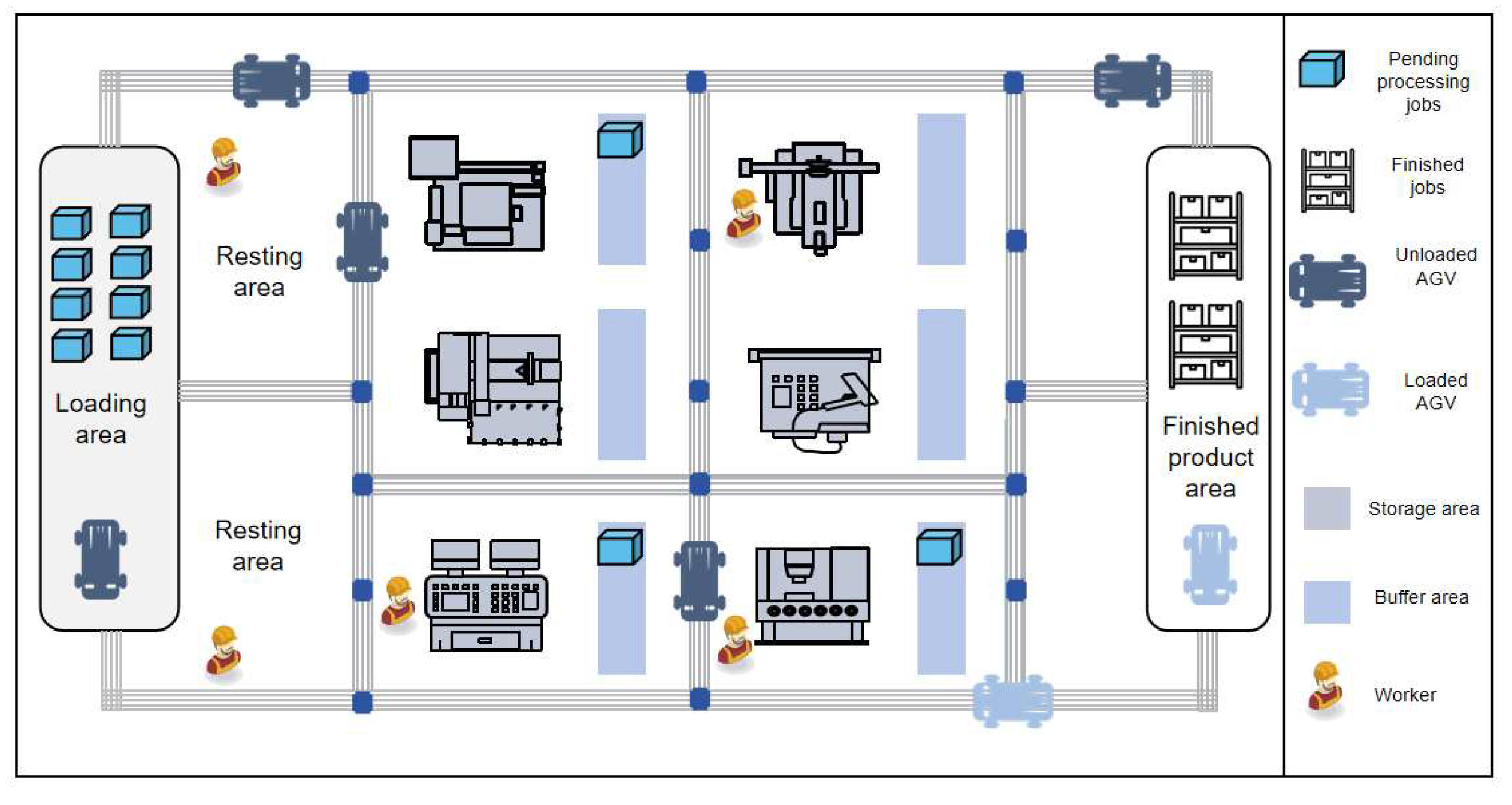
Figure 2.
GWO hierarchical categories.
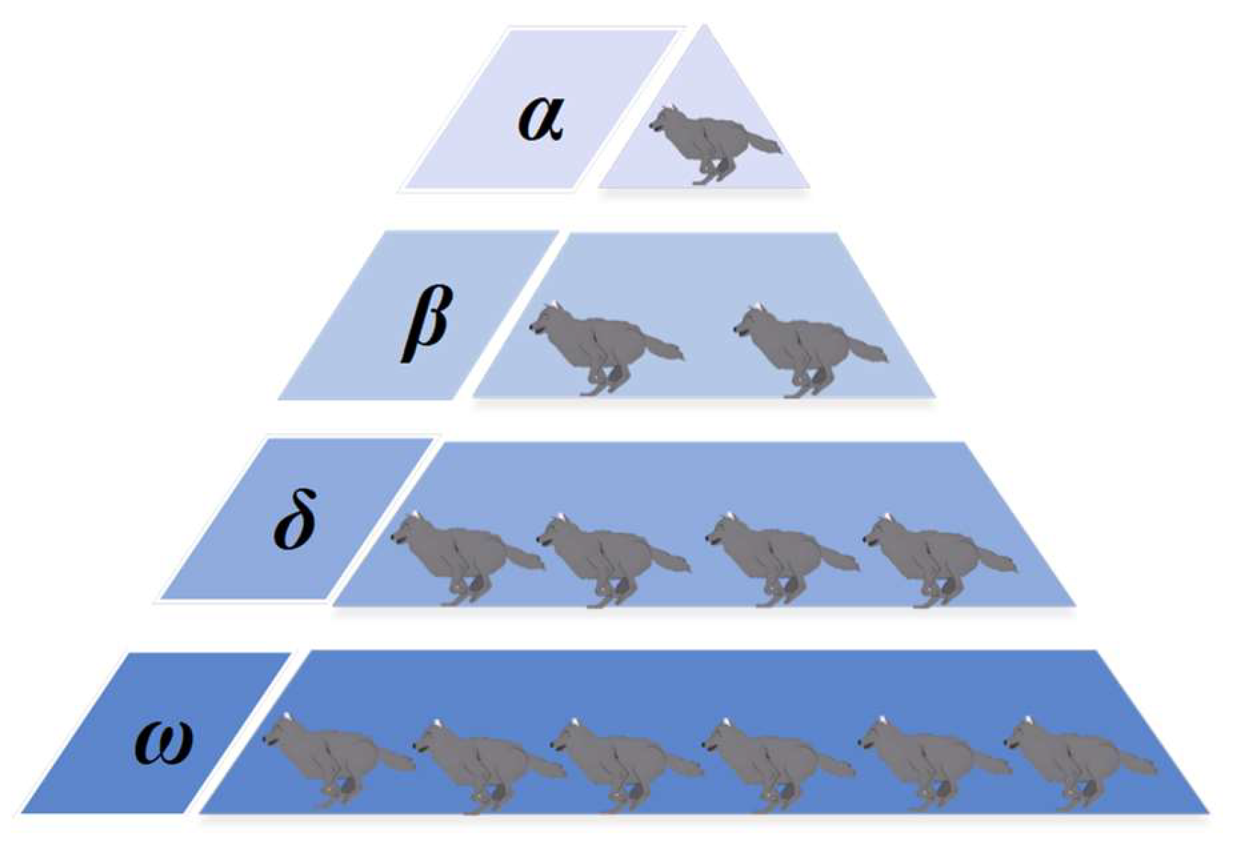
Figure 3.
Figure 3. Individual encoding example: (a) OS vector, (b) MS vector, (c) WS vector, (d) AS vector.
Figure 3.
Figure 3. Individual encoding example: (a) OS vector, (b) MS vector, (c) WS vector, (d) AS vector.
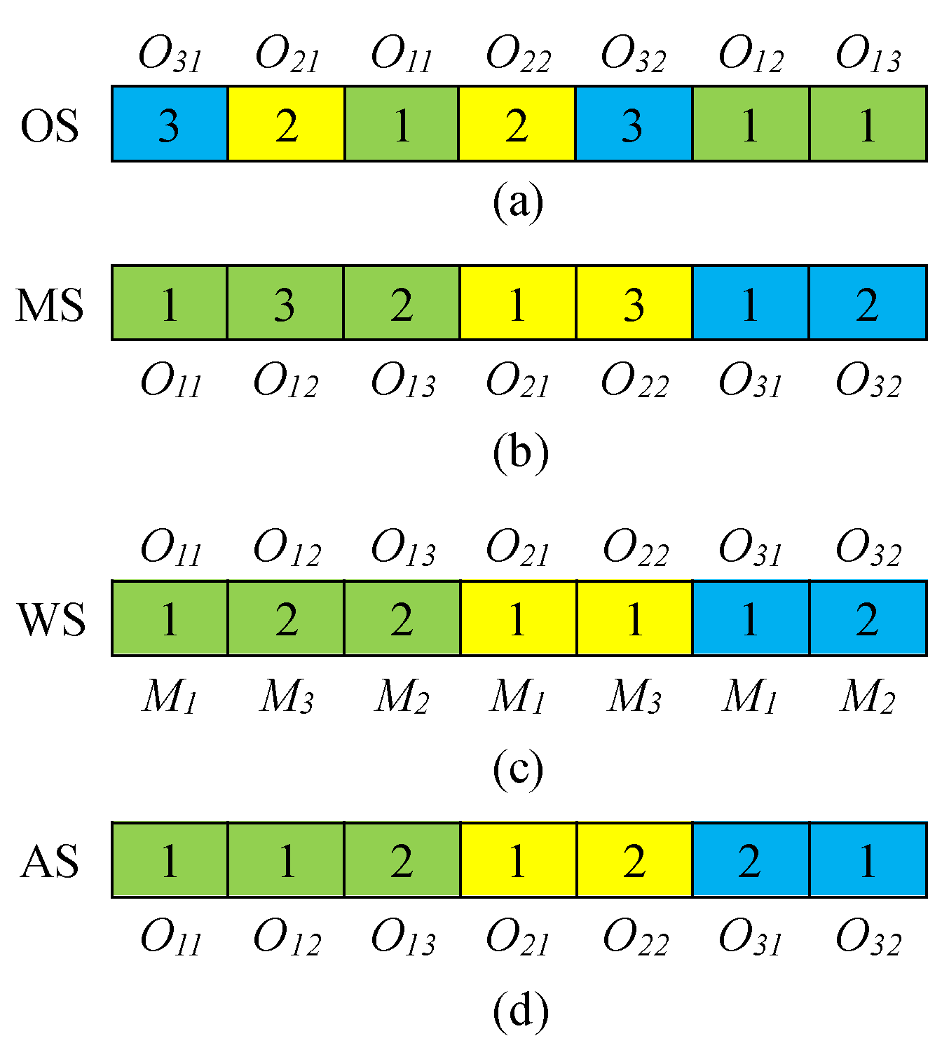
Figure 4.
Updating mechanism for operation sequencing.
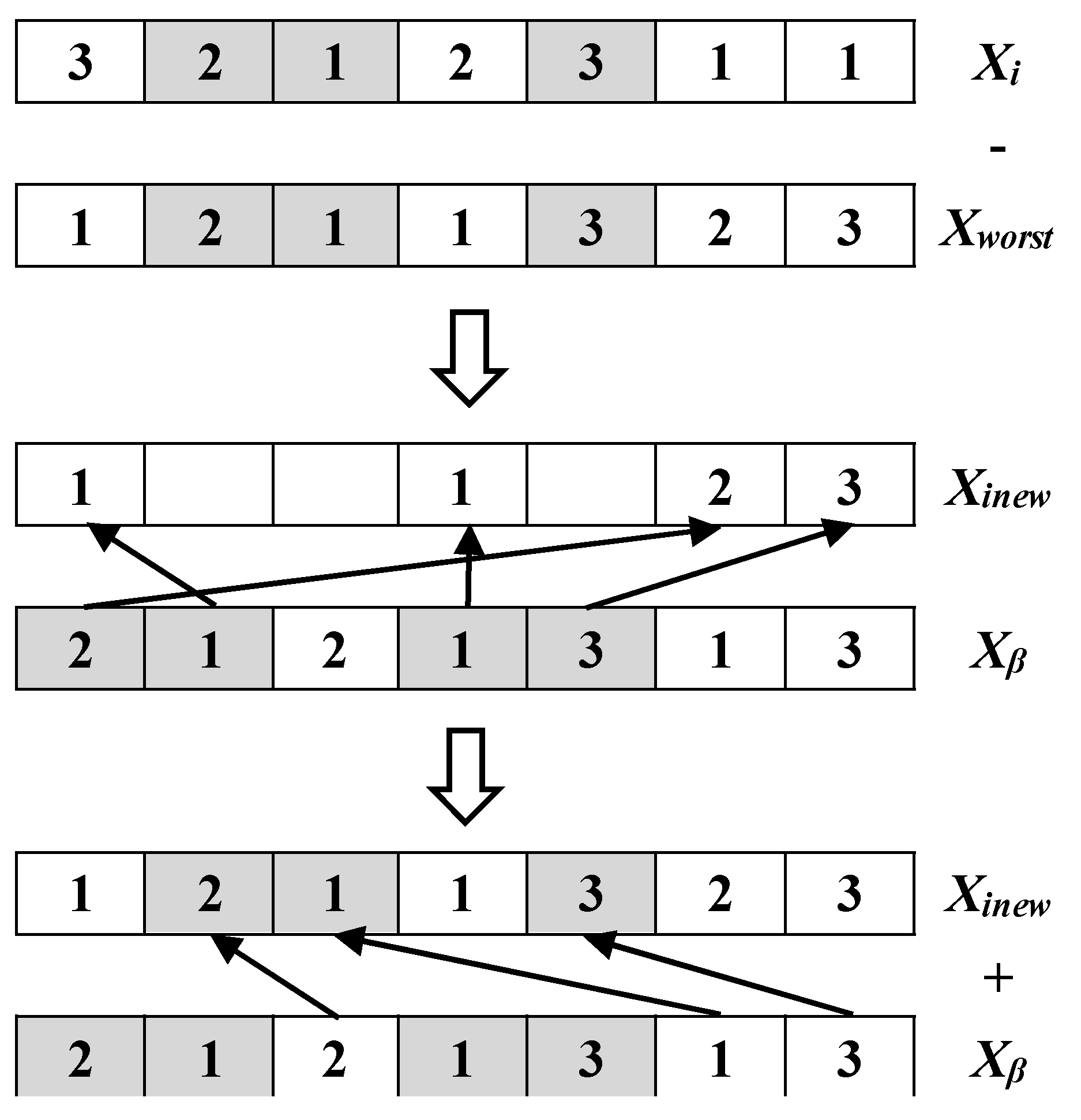
Figure 5.
Updating mechanism for machine selection and AGV selection.
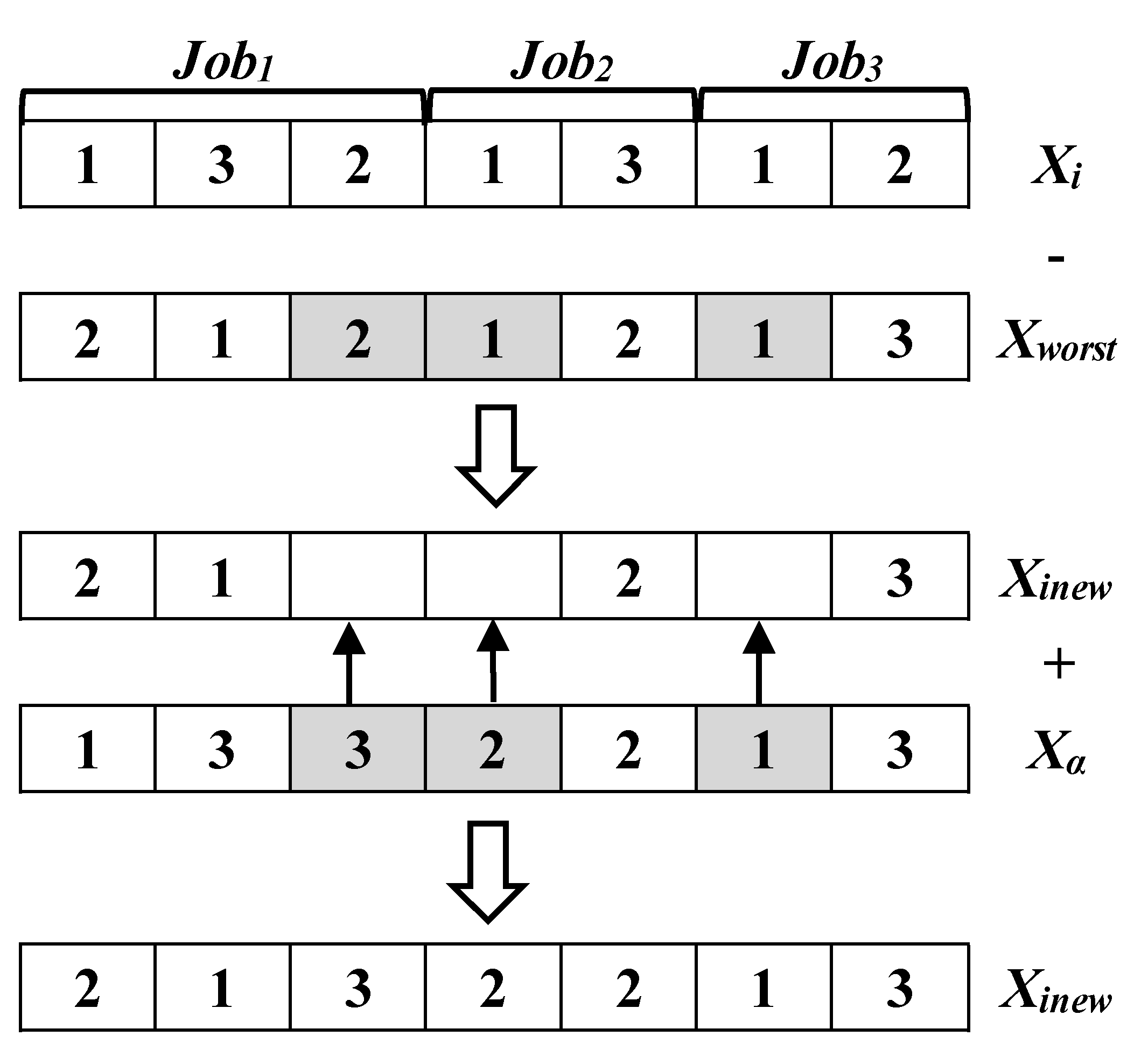
Figure 6.
VNS1 neighborhood search process.
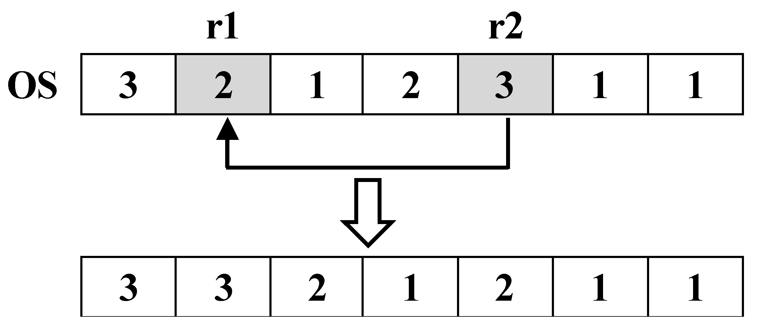
Figure 7.
VNS2 neighborhood search process.
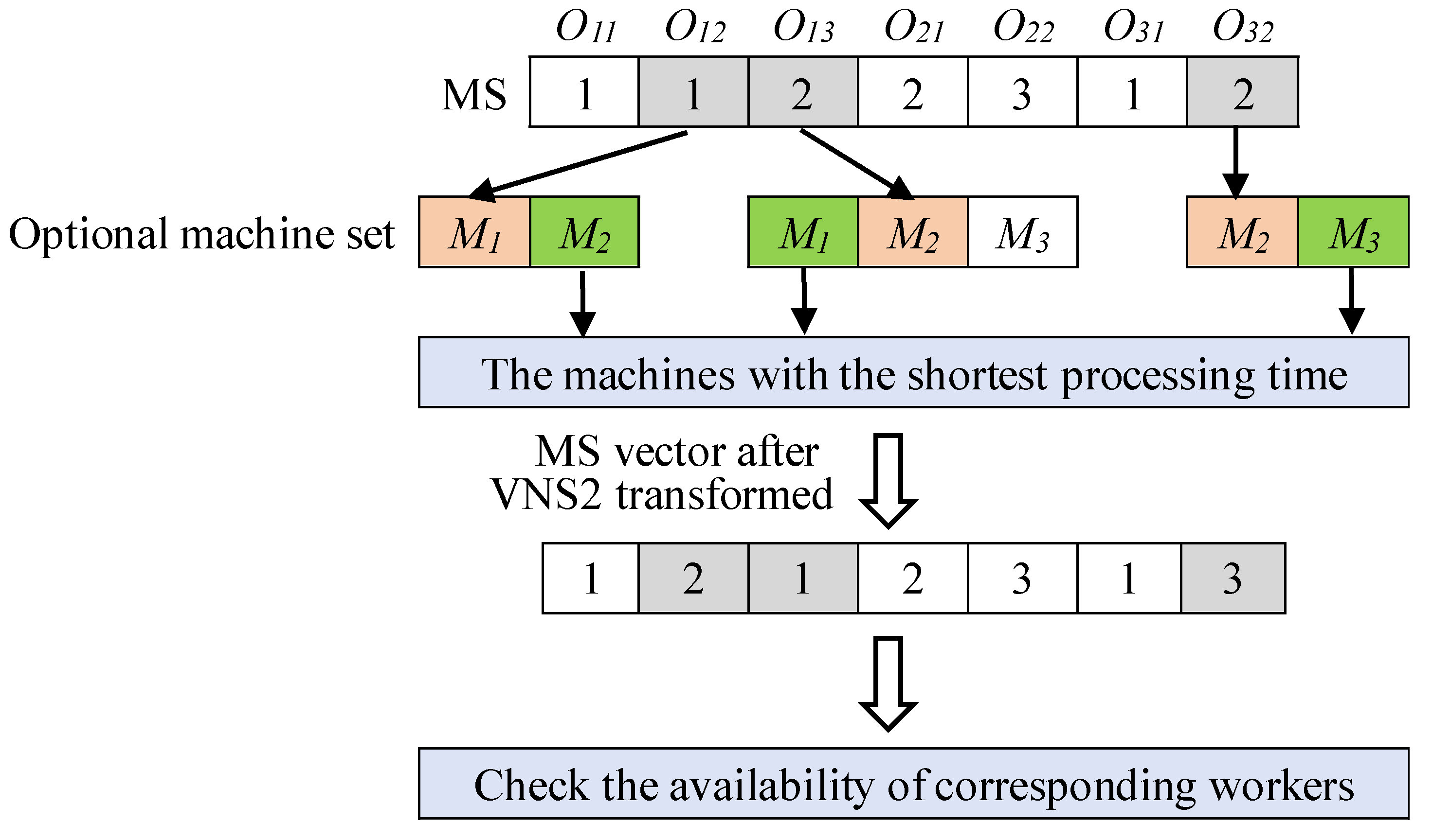
Figure 8.
VNS3 neighborhood search process.
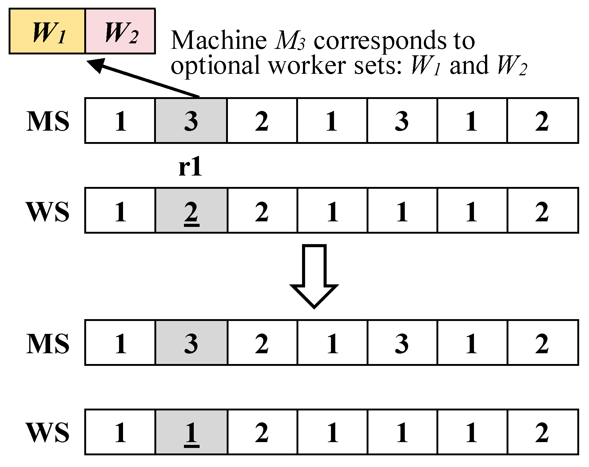
Figure 9.
VNS4 neighborhood search process.
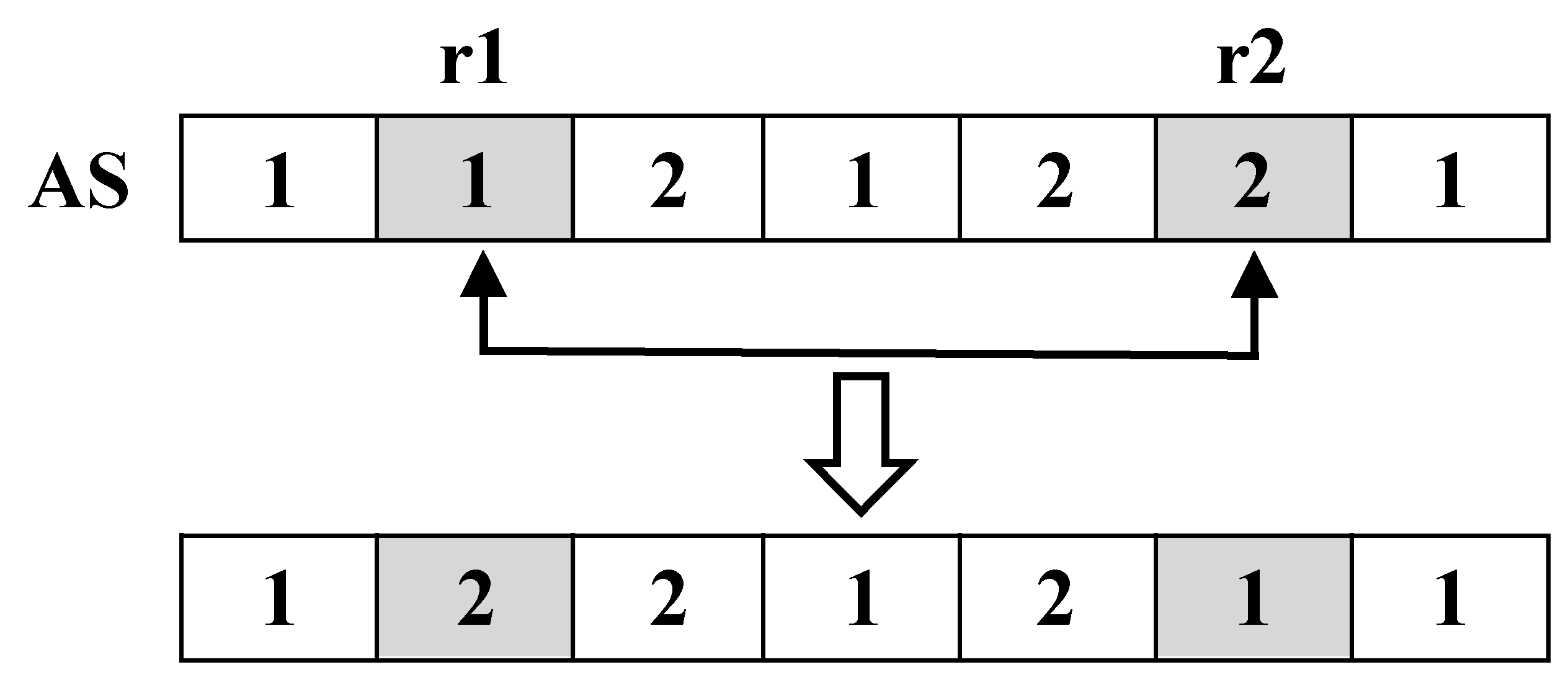
Figure 10.
Box plots for (a) IGD metric and (b) HV metric from Table 5.
Figure 10.
Box plots for (a) IGD metric and (b) HV metric from Table 5.
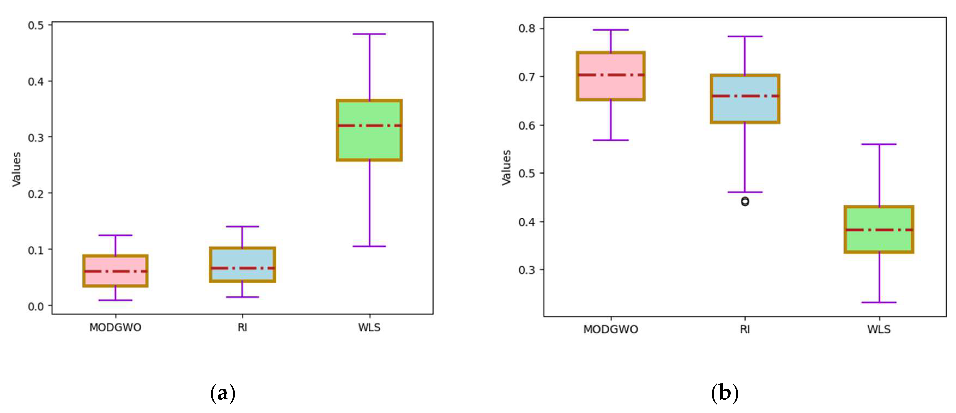
Figure 11.
Comparison of performance of algorithms on small scale instances based on (a) IGD. (b) HV.
Figure 11.
Comparison of performance of algorithms on small scale instances based on (a) IGD. (b) HV.
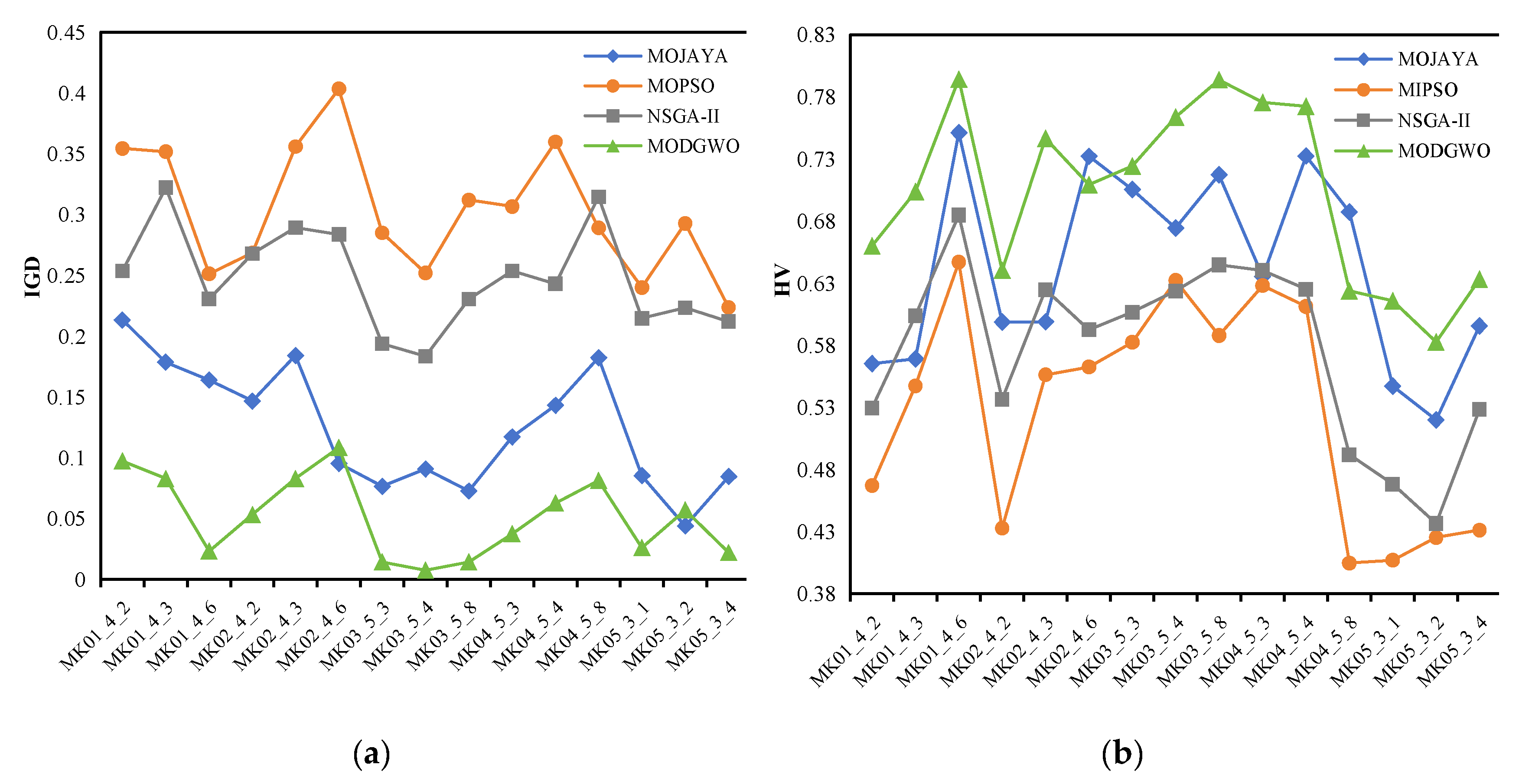
Figure 12.
Comparison of performance of algorithms on medium scale instances based on (a) IGD. (b) HV.
Figure 12.
Comparison of performance of algorithms on medium scale instances based on (a) IGD. (b) HV.
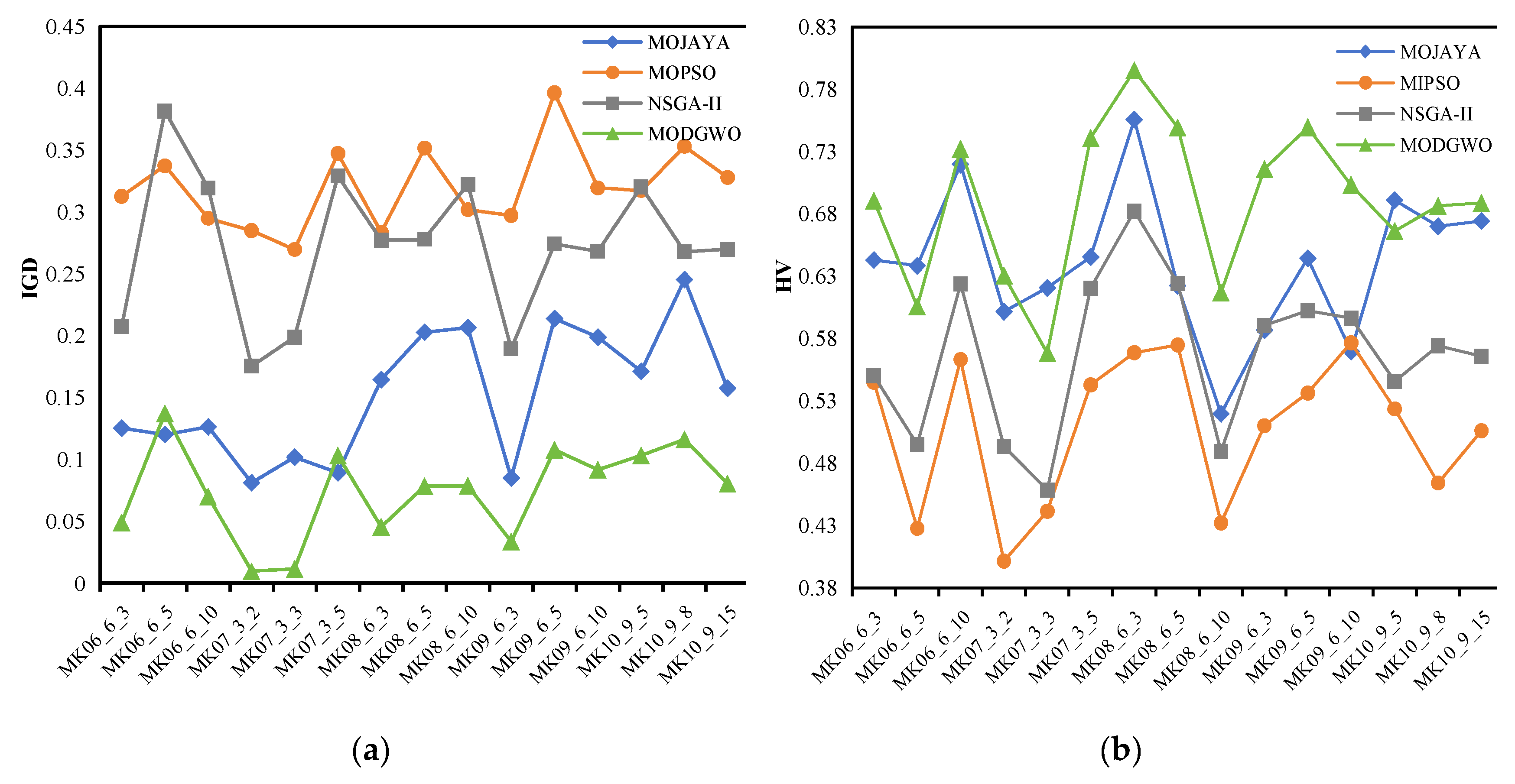
Figure 13.
Comparison of performance of algorithms on large scale instances based on (a) IGD. (b) HV.
Figure 13.
Comparison of performance of algorithms on large scale instances based on (a) IGD. (b) HV.
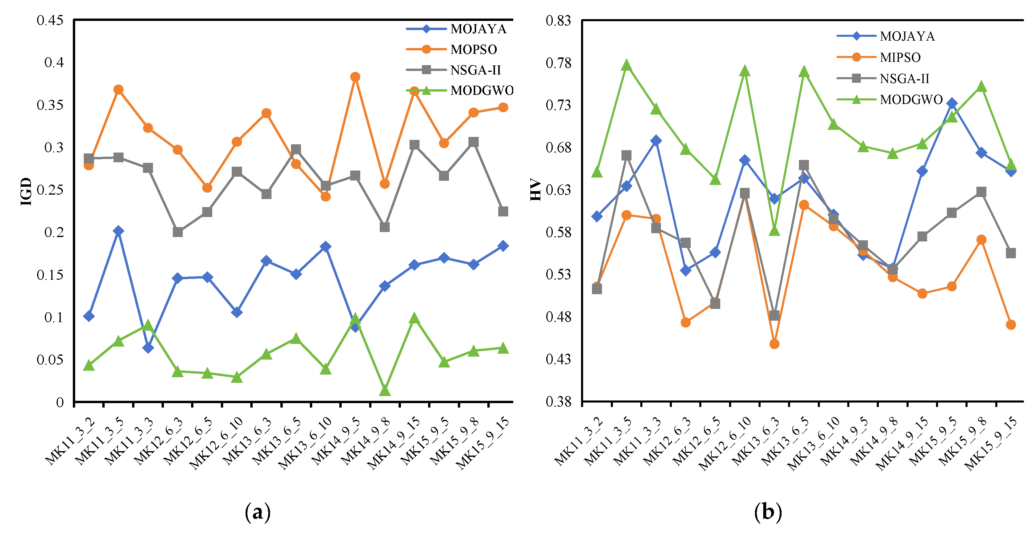
Figure 14.
Scheduling Gantt chart of MK05_3_4.
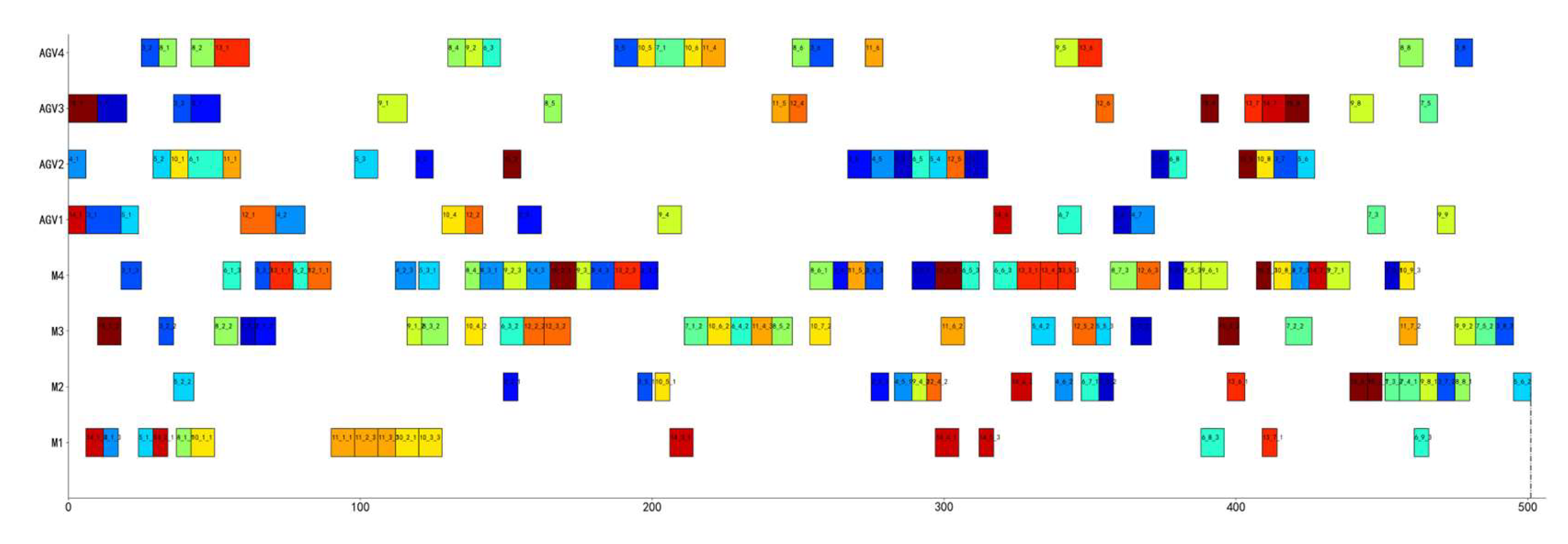
Figure 15.
Gantt charts of two scheduling schemes (a) Single-objective scheduling considering only makespan from the perspective of workers; (b) Dual objective scheduling considering the continuous working hours of workers from the perspective of workers.
Figure 15.
Gantt charts of two scheduling schemes (a) Single-objective scheduling considering only makespan from the perspective of workers; (b) Dual objective scheduling considering the continuous working hours of workers from the perspective of workers.
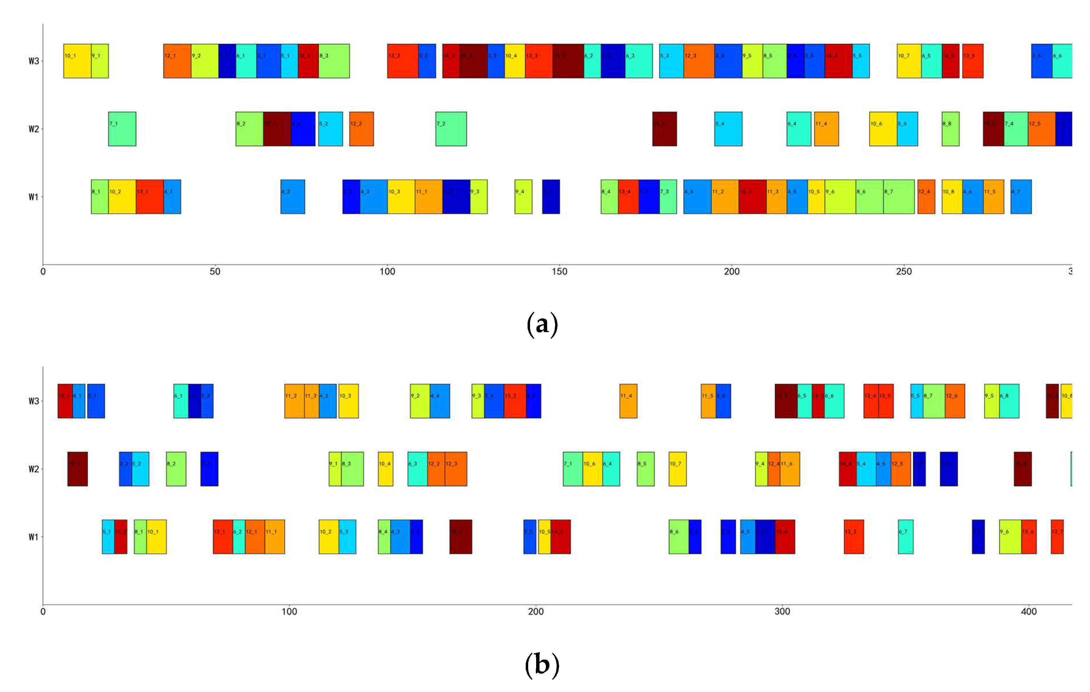
Figure 16.
Distribution diagram of Pareto solutions.
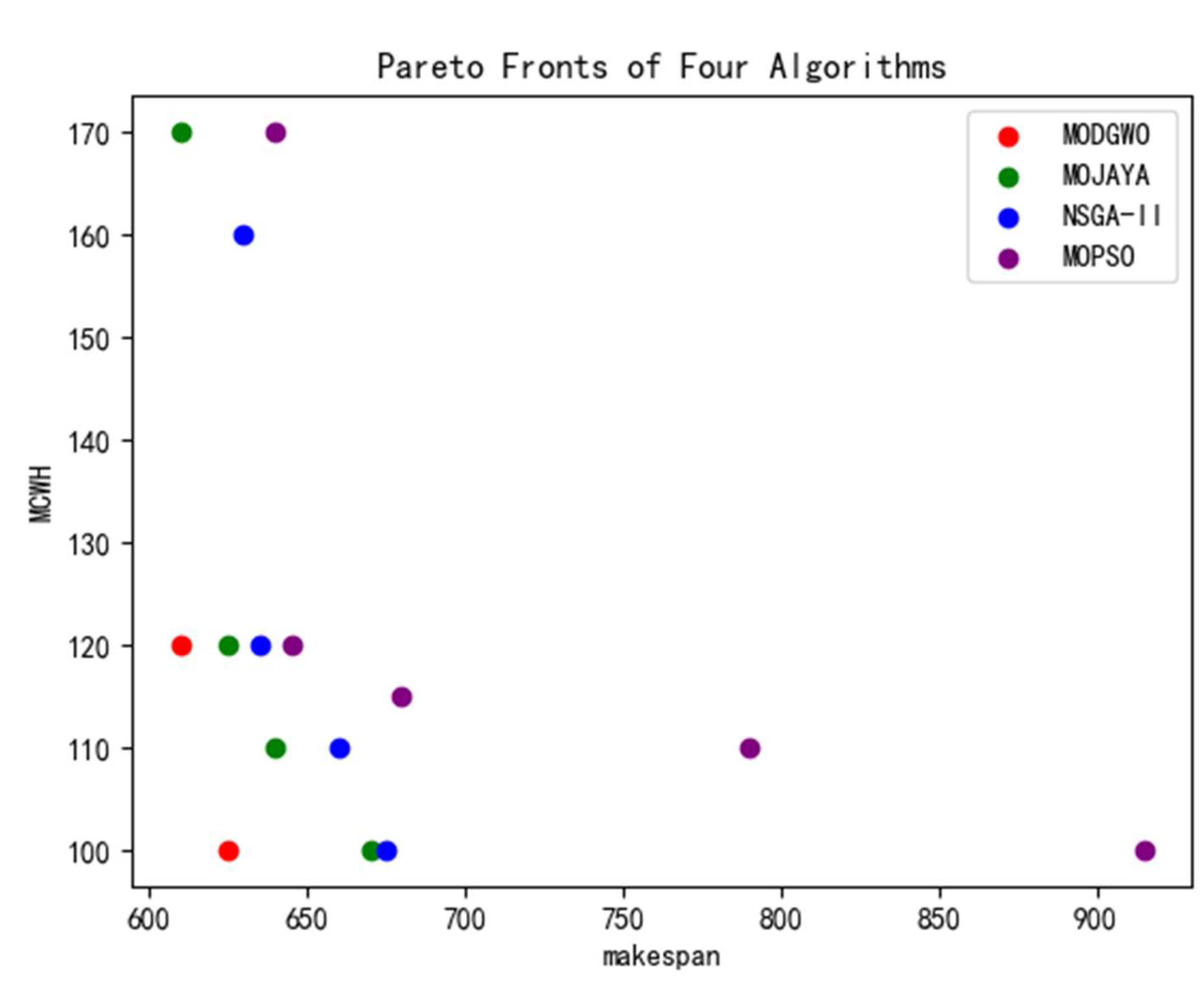

Table 1.
Variables definition and symbols description.
| Notation | Description |
| Indexes andSet | |
| i,i’,h | index of jobs, i,i’,h∈{1,2,...,n} |
| j,j’,g | index of operations, j,j’,g∈{1,2,...,ri} |
| k,q | index of machines, k,q∈{1,2,...,m} |
| s,r | index of workers, s,r∈{1,2,...,l} |
| v | index of AVGs, v∈{1,2,...,w} |
| Ji | The ith job |
| Mk | The kth machine |
| Ws | The sth worker |
| Vv | The vth AVG |
| Oij | The jth operation of Ji |
| Ωij | The set of compatible machines of Oij |
| λk | The set of compatible workers of Mk |
| Parameters | |
| n | Number of total jobs |
| ri | Number of operation of Ji |
| m | Number of total machines |
| l | Number of total workers |
| w | Number of total AVGs |
| Pijks | The processing time of Oij on Mk operated by Ws |
| STij | The start time of Oij |
| CTij | The completion time of Oij |
| Ck | The completion time of Mk |
| STijv | The start time of AGV Vv when transporting Oij |
| CTijv | The completion time of AGV Vv when transporting Oij |
| tgk | Delivery time of AGV Vv from machine Mg to machine Mk |
| Ts | Maximum continuous working hours for worker Ws |
| L | a sufficiently large positive integer |
| Decision variables | |
| xijk | a binary variable: if Oij is assigned on Mk , xijk= 1, otherwise xijk = 0 |
| xijks | a binary variable: if Oij is assigned on Mk operated by Ws, xijks= 1, otherwise xijks = 0 |
| yiji’j’ks | a binary variable: if Oij is ahead of Oi’j’ assigned on Mk operated by Ws, yiji’j’ks= 1, otherwise yiji’j’ks = 0 |
| ziji’j’k | a binary variable: if Oij is ahead of Oi’j’ assigned on Mk , ziji’j’k= 1, otherwise ziji’j’k = 0 |
| αijv | a binary variable: if Oij is transported by AVG Vv , αijv= 1, otherwise αijv = 0 |
| βiji’j’v | a binary variable: if Oij is ahead of Oi’j’ transported by AVG Vv , βiji’j’v=1, otherwise βiji’j’v=0 |
Table 2.
Processing time.
| Job | Operation | Processing time | ||
| M1 | M2 | M3 | ||
| J1 | O11 | 2 | 3 | - |
| O12 | 2 | - | 1 | |
| O13 | 3 | 4 | 3 | |
| J2 | O21 | 1 | 3 | - |
| O22 | - | 2 | 2 | |
| J3 | O31 | 5 | - | 7 |
| O32 | - | 8 | 6 | |
Table 3.
Table 3. Worker-operated machines.
| W1 | W2 | |
| M1 | √ | - |
| M2 | - | √ |
| M3 | √ | √ |
Table 4.
Information of the instances.
| Instance ID | Scale(n×m) | Number of workers | Number ofAVGs |
| MK01 | 10×6 | 4 | 2, 3, 6 |
| MK02 | 10×6 | 4 | 2, 3, 6 |
| MK03 | 15×8 | 5 | 3, 4, 8 |
| MK04 | 15×8 | 5 | 3, 4, 8 |
| MK05 | 15×4 | 3 | 1, 2, 4 |
| MK06 | 10×10 | 6 | 3, 5, 10 |
| MK07 | 20×5 | 3 | 2, 3, 5 |
| MK08 | 20×10 | 6 | 3, 5, 10 |
| MK09 | 20×10 | 6 | 3, 5, 10 |
| MK10 | 20×15 | 9 | 5, 8, 15 |
| MK11 | 30×5 | 3 | 2, 3, 5 |
| MK12 | 30×10 | 6 | 3, 5, 10 |
| MK13 | 30×10 | 6 | 3, 5, 10 |
| MK14 | 30×15 | 9 | 5, 8, 15 |
| MK15 | 30×15 | 9 | 5, 8, 15 |
Table 5.
Performance Comparison between MODGWO, RI and WLS.
| Instance ID | IGD | HV | |||||
| MODGWO | RI | WLS | MODGWO | RI | WLS | ||
| MK01_4_2 | 0.0919 | 0.1085 | 0.2587 | 0.6601 | 0.6194 | 0.3813 | |
| MK01_4_3 | 0.0341 | 0.0258 | 0.1066 | 0.7038 | 0.7255 | 0.3099 | |
| MK01_4_6 | 0.0298 | 0.0595 | 0.3416 | 0.7943 | 0.7536 | 0.5588 | |
| MK02_4_2 | 0.0249 | 0.0456 | 0.2040 | 0.6404 | 0.7204 | 0.3349 | |
| MK02_4_3 | 0.0091 | 0.0146 | 0.1039 | 0.7466 | 0.7176 | 0.5290 | |
| MK02_4_6 | 0.0693 | 0.0941 | 0.3108 | 0.7093 | 0.7023 | 0.3623 | |
| MK03_5_3 | 0.1085 | 0.0994 | 0.2941 | 0.7244 | 0.7582 | 0.4103 | |
| MK03_5_4 | 0.0585 | 0.0672 | 0.3206 | 0.7638 | 0.6609 | 0.3661 | |
| MK03_5_8 | 0.0873 | 0.0611 | 0.3032 | 0.7939 | 0.7022 | 0.4098 | |
| MK04_5_3 | 0.0838 | 0.1041 | 0.4440 | 0.7756 | 0.7047 | 0.5579 | |
| MK04_5_4 | 0.0208 | 0.0385 | 0.2965 | 0.7724 | 0.7018 | 0.4028 | |
| MK04_5_8 | 0.0604 | 0.0403 | 0.3118 | 0.6237 | 0.6935 | 0.4174 | |
| MK05_3_1 | 0.0496 | 0.0621 | 0.3322 | 0.6158 | 0.5725 | 0.2878 | |
| MK05_3_2 | 0.0653 | 0.0586 | 0.4328 | 0.5828 | 0.4430 | 0.3592 | |
| MK05_3_4 | 0.0220 | 0.0385 | 0.2061 | 0.6333 | 0.5146 | 0.3680 | |
| MK06_6_3 | 0.1065 | 0.1311 | 0.3859 | 0.6906 | 0.6298 | 0.4645 | |
| MK06_6_5 | 0.0987 | 0.1197 | 0.4437 | 0.6058 | 0.4608 | 0.2340 | |
| MK06_6_10 | 0.0565 | 0.0694 | 0.2122 | 0.7321 | 0.6329 | 0.4171 | |
| MK07_3_2 | 0.0926 | 0.1123 | 0.3348 | 0.6305 | 0.5279 | 0.3358 | |
| MK07_3_3 | 0.0585 | 0.0670 | 0.3647 | 0.5685 | 0.4399 | 0.2629 | |
| MK07_3_5 | 0.0966 | 0.1033 | 0.4429 | 0.7409 | 0.7828 | 0.5083 | |
| MK08_6_3 | 0.1008 | 0.1176 | 0.3291 | 0.7952 | 0.7656 | 0.4415 | |
| MK08_6_5 | 0.0770 | 0.0977 | 0.2344 | 0.7493 | 0.6188 | 0.3711 | |
| MK08_6_10 | 0.0792 | 0.0952 | 0.3526 | 0.6171 | 0.6046 | 0.2311 | |
| MK09_6_3 | 0.0457 | 0.0538 | 0.3173 | 0.7160 | 0.6342 | 0.3227 | |
| MK09_6_5 | 0.0359 | 0.0412 | 0.3259 | 0.7495 | 0.6690 | 0.4145 | |
| MK09_6_10 | 0.0155 | 0.0355 | 0.3259 | 0.7033 | 0.6923 | 0.4733 | |
| MK10_9_5 | 0.1242 | 0.1395 | 0.3674 | 0.6663 | 0.6284 | 0.3925 | |
| MK10_9_8 | 0.0426 | 0.0680 | 0.2490 | 0.6864 | 0.6599 | 0.3530 | |
| MK10_9_15 | 0.0416 | 0.0628 | 0.2571 | 0.6888 | 0.7554 | 0.3711 | |
| MK11_3_2 | 0.0171 | 0.0426 | 0.3503 | 0.6513 | 0.6407 | 0.3360 | |
| MK11_3_5 | 0.0441 | 0.0513 | 0.4000 | 0.7777 | 0.6842 | 0.5382 | |
| MK11_3_3 | 0.0694 | 0.0941 | 0.2872 | 0.7257 | 0.6272 | 0.5121 | |
| MK12_6_3 | 0.0785 | 0.0930 | 0.2593 | 0.6782 | 0.5767 | 0.3459 | |
| MK12_6_5 | 0.0808 | 0.1079 | 0.4347 | 0.6425 | 0.5650 | 0.4217 | |
| MK12_6_10 | 0.1113 | 0.1365 | 0.4819 | 0.7708 | 0.7509 | 0.4145 | |
| MK13_6_3 | 0.0533 | 0.0611 | 0.2760 | 0.5823 | 0.6512 | 0.2344 | |
| MK13_6_5 | 0.0670 | 0.0943 | 0.3321 | 0.7700 | 0.6634 | 0.5513 | |
| MK13_6_10 | 0.0135 | 0.0234 | 0.3950 | 0.7075 | 0.6767 | 0.3673 | |
| MK14_9_5 | 0.0080 | 0.0196 | 0.2478 | 0.6811 | 0.5930 | 0.3006 | |
| MK14_9_8 | 0.0237 | 0.0390 | 0.2242 | 0.6731 | 0.5487 | 0.4462 | |
| MK14_9_15 | 0.0100 | 0.0373 | 0.3446 | 0.6845 | 0.6180 | 0.3912 | |
| MK15_9_5 | 0.1029 | 0.1132 | 0.2900 | 0.7163 | 0.7033 | 0.3343 | |
| MK15_9_8 | 0.0745 | 0.0859 | 0.2558 | 0.7524 | 0.6647 | 0.4298 | |
| MK15_9_15 | 0.0874 | 0.1023 | 0.3954 | 0.6601 | 0.5603 | 0.3834 | |
Table 6.
Performance Comparison between MOJAYA, MOPSO, NSGAⅡand MODGWO.
| Instance ID | MOJAYA | MOPSO | NSGA-II | MODGWO | |||||||
| IGD | HV | IGD | HV | IGD | HV | IGD | HV | ||||
| MK01_4_2 | 0.2132 | 0.5653 | 0.3544 | 0.4671 | 0.2536 | 0.5295 | 0.0973 | 0.6601 | |||
| MK01_4_3 | 0.1785 | 0.5690 | 0.3518 | 0.5474 | 0.3222 | 0.6038 | 0.0829 | 0.7038 | |||
| MK01_4_6 | 0.1640 | 0.7512 | 0.2513 | 0.6470 | 0.2306 | 0.6849 | 0.0231 | 0.7943 | |||
| MK02_4_2 | 0.1466 | 0.5988 | 0.2687 | 0.4327 | 0.2679 | 0.5365 | 0.0532 | 0.6404 | |||
| MK02_4_3 | 0.1840 | 0.5989 | 0.3560 | 0.5562 | 0.2893 | 0.6248 | 0.0829 | 0.7466 | |||
| MK02_4_6 | 0.0953 | 0.7322 | 0.4035 | 0.5626 | 0.2837 | 0.5925 | 0.1083 | 0.7093 | |||
| MK03_5_3 | 0.0765 | 0.7054 | 0.2851 | 0.5825 | 0.1938 | 0.6067 | 0.0142 | 0.7244 | |||
| MK03_5_4 | 0.0907 | 0.6745 | 0.2520 | 0.6323 | 0.1835 | 0.6237 | 0.0075 | 0.7638 | |||
| MK03_5_8 | 0.0726 | 0.7174 | 0.3120 | 0.5879 | 0.2304 | 0.6448 | 0.0143 | 0.7939 | |||
| MK04_5_3 | 0.1170 | 0.6352 | 0.3066 | 0.6282 | 0.2536 | 0.6404 | 0.0374 | 0.7756 | |||
| MK04_5_4 | 0.1431 | 0.7325 | 0.3598 | 0.6113 | 0.2431 | 0.6251 | 0.0628 | 0.7724 | |||
| MK04_5_8 | 0.1822 | 0.6874 | 0.2891 | 0.4046 | 0.3145 | 0.4919 | 0.0812 | 0.6237 | |||
| MK05_3_1 | 0.0851 | 0.5472 | 0.2400 | 0.4069 | 0.2147 | 0.4681 | 0.0260 | 0.6158 | |||
| MK05_3_2 | 0.0438 | 0.5199 | 0.2927 | 0.4252 | 0.2233 | 0.4365 | 0.0571 | 0.5828 | |||
| MK05_3_4 | 0.0844 | 0.5955 | 0.2237 | 0.4312 | 0.2121 | 0.5284 | 0.0220 | 0.6333 | |||
| MK06_6_3 | 0.1255 | 0.6431 | 0.3127 | 0.5452 | 0.2074 | 0.5504 | 0.0490 | 0.6906 | |||
| MK06_6_5 | 0.1203 | 0.6384 | 0.3374 | 0.4279 | 0.3816 | 0.4952 | 0.1372 | 0.6058 | |||
| MK06_6_10 | 0.1263 | 0.7197 | 0.2949 | 0.5633 | 0.3194 | 0.6240 | 0.0700 | 0.7321 | |||
| MK07_3_2 | 0.0812 | 0.6016 | 0.2850 | 0.4016 | 0.1756 | 0.4938 | 0.0097 | 0.6305 | |||
| MK07_3_3 | 0.1020 | 0.6207 | 0.2697 | 0.4417 | 0.1989 | 0.4586 | 0.0116 | 0.5685 | |||
| MK07_3_5 | 0.0893 | 0.6456 | 0.3473 | 0.5429 | 0.3292 | 0.6204 | 0.1033 | 0.7409 | |||
| MK08_6_3 | 0.1645 | 0.7556 | 0.2837 | 0.5688 | 0.2773 | 0.6824 | 0.0457 | 0.7952 | |||
| MK08_6_5 | 0.2029 | 0.6224 | 0.3517 | 0.5749 | 0.2783 | 0.6244 | 0.0785 | 0.7493 | |||
| MK08_6_10 | 0.2067 | 0.5198 | 0.3019 | 0.4323 | 0.3225 | 0.4896 | 0.0787 | 0.6171 | |||
| MK09_6_3 | 0.0852 | 0.5868 | 0.2973 | 0.5102 | 0.1896 | 0.5907 | 0.0336 | 0.7160 | |||
| MK09_6_5 | 0.2139 | 0.6444 | 0.3963 | 0.5363 | 0.2742 | 0.6025 | 0.1080 | 0.7495 | |||
| MK09_6_10 | 0.1990 | 0.5699 | 0.3195 | 0.5767 | 0.2683 | 0.5964 | 0.0918 | 0.7033 | |||
| MK10_9_5 | 0.1711 | 0.6909 | 0.3173 | 0.5237 | 0.3204 | 0.5457 | 0.1032 | 0.6663 | |||
| MK10_9_8 | 0.2454 | 0.6700 | 0.3531 | 0.4643 | 0.2680 | 0.5742 | 0.1164 | 0.6864 | |||
| MK10_9_15 | 0.1575 | 0.6744 | 0.3280 | 0.5062 | 0.2698 | 0.5660 | 0.0805 | 0.6888 | |||
| MK11_3_2 | 0.1010 | 0.5984 | 0.2786 | 0.5153 | 0.2866 | 0.5125 | 0.0435 | 0.6513 | |||
| MK11_3_5 | 0.2013 | 0.6342 | 0.3677 | 0.5999 | 0.2878 | 0.6703 | 0.0720 | 0.7777 | |||
| MK11_3_3 | 0.0638 | 0.6879 | 0.3226 | 0.5954 | 0.2754 | 0.5845 | 0.0909 | 0.7257 | |||
| MK12_6_3 | 0.1458 | 0.5345 | 0.2969 | 0.4730 | 0.1998 | 0.5669 | 0.0361 | 0.6782 | |||
| MK12_6_5 | 0.1470 | 0.5558 | 0.2521 | 0.4972 | 0.2236 | 0.4950 | 0.0342 | 0.6425 | |||
| MK12_6_10 | 0.1055 | 0.6647 | 0.3062 | 0.6239 | 0.2711 | 0.6259 | 0.0295 | 0.7708 | |||
| MK13_6_3 | 0.1662 | 0.6192 | 0.3400 | 0.4477 | 0.2445 | 0.4810 | 0.0567 | 0.5823 | |||
| MK13_6_5 | 0.1504 | 0.6436 | 0.2801 | 0.6118 | 0.2972 | 0.6589 | 0.0750 | 0.7700 | |||
| MK13_6_10 | 0.1830 | 0.6003 | 0.2417 | 0.5868 | 0.2545 | 0.5952 | 0.0392 | 0.7075 | |||
| MK14_9_5 | 0.0883 | 0.5527 | 0.3827 | 0.5578 | 0.2664 | 0.5641 | 0.0989 | 0.6811 | |||
| MK14_9_8 | 0.1366 | 0.5366 | 0.2568 | 0.5266 | 0.2056 | 0.5357 | 0.0142 | 0.6731 | |||
| MK14_9_15 | 0.1614 | 0.6520 | 0.3658 | 0.5071 | 0.3027 | 0.5745 | 0.0995 | 0.6845 | |||
| MK15_9_5 | 0.1697 | 0.7319 | 0.3046 | 0.5157 | 0.2661 | 0.6026 | 0.0473 | 0.7163 | |||
| MK15_9_8 | 0.1618 | 0.6735 | 0.3407 | 0.5709 | 0.3061 | 0.6273 | 0.0604 | 0.7524 | |||
| MK15_9_15 | 0.1838 | 0.6515 | 0.3467 | 0.4704 | 0.2242 | 0.5548 | 0.0639 | 0.6601 | |||
Table 7.
The set of machines that can be operated by workers in case MK05_3_4.
| Worker Number | The set of machines operated by workers |
| W1 | {M1, M2, M4} |
| W2 | {M2, M3} |
| W3 | {M1, M3, M4} |
Table 8.
Machine information.
| Machine name | Machine number |
| CNC lathe | M1 |
| M2 | |
| Laser cutting machine | M3 |
| Automatic straightening machine | M4 |
| spray painting robot | M5 |
| M6 | |
| CNC milling machine | M7 |
| CNC grinding machine | M8 |
| High frequency quenching machine | M9 |
| Forging machine | M10 |
| M11 |
Table 9.
Operation processing information.
| Job | Operation | Operation name | Machine | Processing time |
| Shaftless soil conveyor pig iron roller pin | O11 | Milling | M7 | 50 |
| O12 | Grinding | M8 | 70 | |
| O13 | High Frequency Hardening | M9 | 120 | |
| Soil covered guide frame suspension rod | O21 | Cutting | M3 | 150 |
| O22 | Sandblasting | M5/M6 | 80/65 | |
| O23 | Straightening | M4 | 40 | |
| Extinguisher Traction Column | O31 | Forging | M10/M11 | 50/40 |
| O32 | Turning | M1/M2 | 130/110 | |
| O33 | Grinding | M8 | 70 | |
| O34 | Sandblasting | M5/M6 | 75/60 | |
| Short Wheel tail pin | O41 | Forging | M10/M11 | 20/10 |
| O42 | CNC Turning | M1/M2 | 90/70 | |
| O43 | CNC Grinding | M8 | 65 | |
| O44 | Sandblasting | M5/M6 | 50/35 | |
| Long four-bar linkage pin | O51 | Forging | M10/M11 | 35/25 |
| O52 | rough machining | M1/M2 | 80/60 | |
| O53 | fine machining | M1/M2 | 60/40 | |
| O54 | High Frequency Hardening | M9 | 100 |
Table 10.
The transportation time between each machine and the LU area.
| LU | M1 | M2 | M3 | M4 | M5 | M6 | M7 | M8 | M9 | M10 | M11 | |
| LU | 0 | 10 | 20 | 30 | 25 | 35 | 45 | 15 | 25 | 35 | 30 | 40 |
| M1 | 10 | 0 | 5 | 30 | 50 | 60 | 70 | 40 | 50 | 60 | 100 | 110 |
| M2 | 20 | 5 | 0 | 30 | 50 | 60 | 70 | 40 | 50 | 60 | 100 | 110 |
| M3 | 30 | 30 | 30 | 0 | 20 | 10 | 20 | 50 | 60 | 70 | 110 | 120 |
| M4 | 25 | 50 | 50 | 20 | 0 | 30 | 40 | 70 | 80 | 90 | 130 | 140 |
| M5 | 35 | 60 | 60 | 10 | 30 | 0 | 5 | 80 | 90 | 100 | 140 | 150 |
| M6 | 45 | 70 | 70 | 20 | 40 | 5 | 0 | 90 | 100 | 110 | 150 | 160 |
| M7 | 15 | 40 | 40 | 50 | 70 | 80 | 90 | 0 | 10 | 20 | 60 | 70 |
| M8 | 25 | 50 | 50 | 60 | 80 | 90 | 100 | 10 | 0 | 10 | 70 | 80 |
| M9 | 35 | 60 | 60 | 70 | 90 | 100 | 110 | 20 | 10 | 0 | 80 | 90 |
| M10 | 30 | 100 | 100 | 110 | 130 | 140 | 150 | 60 | 70 | 80 | 0 | 5 |
| M11 | 40 | 110 | 110 | 120 | 140 | 150 | 160 | 70 | 80 | 90 | 5 | 0 |
Table 11.
The set of machines that can be operated by workers in the enterprise.
| Worker Number | The set of machines operated by workers |
| W1 | {M1, M2, M5, M6, M10, M11} |
| W2 | {M1, M2, M5, M6, M7} |
| W3 | {M1, M2, M3, M4, M5, M6} |
| W4 | {M3, M4, M8, M10, M11} |
| W5 | {M3, M4, M9, M10, M11} |
| W6 | {M1, M2, M4, M8, M10, M11} |
| W7 | {M1, M2, M5, M6, M9} |
Table 12.
Running results.
| Algorithms | IGD | HV |
| MODGWO | 0.0824 | 0.6457 |
| MOJAYA | 0.1513 | 0.6011 |
| NSGA-II | 0.2932 | 0.5246 |
| MOPSO | 0.3828 | 0.4876 |
Table 13.
Pareto solutions for four algorithms.
| Algorithms | Number of solutions | Pareto solutions |
| MODGWO | 2 | [610, 120],[625, 100] |
| MOJAYA | 4 | [610, 170],[625, 120],[640,110],[670, 100] |
| NSGA-II | 4 | [635, 120],[630,160],[660, 110],[675, 100] |
| MOPSO | 5 | [645, 120],[640,170],[680,115],[790, 110],[915, 100] |
Disclaimer/Publisher’s Note: The statements, opinions and data contained in all publications are solely those of the individual author(s) and contributor(s) and not of MDPI and/or the editor(s). MDPI and/or the editor(s) disclaim responsibility for any injury to people or property resulting from any ideas, methods, instructions or products referred to in the content. |
© 2025 by the authors. Licensee MDPI, Basel, Switzerland. This article is an open access article distributed under the terms and conditions of the Creative Commons Attribution (CC BY) license (http://creativecommons.org/licenses/by/4.0/).
Copyright: This open access article is published under a Creative Commons CC BY 4.0 license, which permit the free download, distribution, and reuse, provided that the author and preprint are cited in any reuse.


