Submitted:
06 September 2025
Posted:
08 September 2025
You are already at the latest version
Abstract
In this paper, we consider a general quadratic problem (P) with linear constraints that are not necessarily linear independent. To resolve this problem, we use a new algorithm based on the Inertia-Controlling method while replacing the condition of Lagrange multiplier vector μ by resolution of linear system obtained thanks to the Kuruch-Kuhn -Tuker matrix (KKT-matrix) in order to determine the minimize direction of (P) and so calculate the steep length in general case: indefinite, concave and convex cases. Moreover, the results presented here mark the end of the approximate methods to quadratic programming as well as the linear complementarity methods of the problems to be studied.
Keywords:
global Solution
; descent direction
; direction of negative curvature
; K KT-matrix
; interior point
; inertia controlling
1. Introduction
Currently, the domain of optimization is attracting considerable interest from the academic and industrial communities, see, for instances [1,2,3]. The various studies existing for solving a given problem in this domain and the efficient algorithmics implementations open up many perspectives and diverse applications. By many researchers in this field and whose objective is formed by several numerical methods [5,6,9] used in two ways; the first way is the essential principal of such a generally method consists of enumerating, often of implicitly manner the set of solutions of the optimization problem as well as has the techniques to detect the possible failures and the second way concerning the large size.
The quadratic programming problem in continuous time and the theory of the characterizations of its global solutions seem appropriate to the questions where the objective function is of the general form either convex, concave or indefinite form. However, the quadratic problem can be written in several forms equivalents, normally, which help us to simplify and find the good optimality conditions for this type of problems in the general case, but now, it’s only found for the general quadratic programming of optimization with equality constraints [10].
According to our long scientific research on the manner for solving our problem denoted in below, we have not found an effective method that will allow us to find the globally minimum in reasonable time and avoiding the numerical difficulties linked to the bad conditioning of the Hessian of problem.
With the new global sufficiently conditions that we propose, we can apply any iterative method converging towards the local solution of the problem (P) whose the goal is to compute the global solutions of the optimization problems (P). As in the indefinite case, the (P) problem, may had more than one global solution, this on the one hand, on the other hand, we avoid writing the equivalent forms to the optimization problem (P) which helps us to take directly the original problem. The analytic solution is computationally intense and numerical issues my occur, knowing, this solution exists especially when the domain is bounded, However it`s not the case with the not indefinite Hessian reduced matrix and the question is stay also posed about the globally solution which is noted by variable .
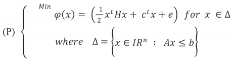
In this study, we are interested on the global sufficiently conditions to solve the general quadratic problem of optimization, where the set of his constraints are linear:
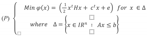
Such as A is an (m∗n) matrix not necessarily full rank; H is a Hessian matrix of order n (not necessarily convex). The b and c are two given vectors, and e is a scalar.
Actually, the conditions which we help to solve the problem (P) are not found. By these conditions we can apply any iterative method converging to the local solution of problem (P), whose goal is to compute the global solution of the optimization problem of (P).
This analytic solution is computationally intense and numerical issues my occur, knowing, this solution exists especially when the domain of constraints is bonded, or not bonded with the reduced Hessian is not indefinite, but the question is stay also posed about the global solution in other cases, for example, in case of indefinite reduced Hessian matrix.
2. Notation and Glossary
We present in this paragraph the designation of the different symbols and variables used in our work:

Table 1.
Notation and Glossary.
| Ak | The active matrix at iteration k |
| m,mk | Number of rows in matrix A respectively Ak |
| Stationary point | |
| Active point | |
| Globally solution | |
| q | Direction of minimization |
| Lagrange Multiplier vector’s | |
| and | denotes respectively the steep length in convex case c and in indefinite case i |
| Zk | Kernel matrix of Ak |
| nk | Number of columns in Zk |
| The objective function | |
| H | The Hessian matrix |
| I. C.M | Denotes the initials letters of Inertia Controlling Method |
| The gradient of objective function in point at iteration k | |
| The domain of linear constraints of problem (P) | |
| Fr () | denotes the domain border of |
| P.D | Denotes the initials letters of Positive Defined matrix |
3. Existence of Global Solution
We consider the general quadratic problem (P) under the linear constraints Δ.
To show the existence of the global solution, we are stating and implementing two lemmas. The first concerns the determination of minimization direction q (negative direction of curvature, or direction of descent). The second concerns the steep of length which makes finite our algorithm.
3.1.
Lemma 1. Let a stationary point obtained at iteration k. Then the following linear system (1) obtained thanks KKT-matrix has a single solution in
Note that this solution exists and unique if and only if matrix, with Zk is a kernel matrix of Ak such that
This single solution is a minimize direction of in the following cases:
Case1 with
Case2 with
Proof
Given that is D.P. matrix, then it is non-singular matrix and according to the expression referred to in [1], it comes to us that the K-matrix
Consequently, the linear system (1) has a single solution .
Now, let’s distinguish the cases where the vector q represents the minimization direction of problem (P).
Let us recall that, among the important properties in general quadratic programming problem and iterates at the point we have [1] (2)
In case1: If with . We have directly .
This fits the negative curvature direction which is a minimization direction
In case2: if with . It fits a descent direction at point and positive curvature. Here it results also
3.2.
Lemma 2. We take the same data of lemma1 with the satisfaction once situation of these two following cases:
Case1 with
Case2 with such that
Where (4)
and (5)
Then is a globally solution of our problem (P).
Proof
Take the expression used in the proof of Lemma 1,
In case1: According the expression that we have considered in proof of lemma 1, it results that
In case 2: As where
We multiply the expression (4) by , it means
.
and involve that it results
This expression is always positive.
That is and according the expression that we have considered in proof of lemma 1
( it results that
and we can say that is a globally solution of problem (P).
4. New Sufficient Conditions Globally Solution of (P)
The new sufficient conditions globally solutions of the problem (P) that we propose are shown in the following steps:
- is a positive defined matrix
- In this third condition we propose the new following step. We replace the condition of Lagrange Multiplier 0 by the following linear system obtained thanks to KKT-Matrix
Which has the only increasing direction q with the steep length
on all cases i.e. in convex case such that
And in indefinite case such that
Where
Proof
Before showing this result, we will recall the sufficient conditions of the local solutions of the problems of type (P) which is given in the following theorem and use his results to find the globally solution:
Theorem [10]
We consider the quadratic problem (P), and let be the point obtained by minimizing the objective function ϕ after performing k iterations starting from the initial point . We are given two matrices, and , such that the columns of the latter constitute a basis for the kernel of the former. If there is a positive vector such that ,
and if more the expression is positive for all
Then is a local solution of the problem (P).
Now, we return to show the proof of the our original result by considering (because the case of is evidently
We have
We multiply by qt; we obtain:
(6)
(who can be positive for a global solution)
We distinguish her two following cases:
Case1. If then we obtain a decreasing direction q from the linear system (1), so the point is not a global solution of problem (P) we therefore continue the calculation until find the best solution.
Case2. If as we have and
two situations appear:
The first: If, then point is a global solution of our (P) problem, where
The second: If then we continue to do the same technical of minimization at the point, until find the global solution .
5. Inertia Controlling Method (I.C.M)
We note that the researchers have abandoned this method, which I believe could be improved and applied to help us solve our problem by introducing some changes (see section 4 in above) to obtain better results, especially since it relies on second-order conditions, whether related to the nature of the reduced Hessian matrix or the nature of the minimization direction.
Definition 1. (Stationary Point) [1]
We say the point = is stationary point of problem (P) if we have these two followings conditions are hold:
- (Positive Defined matrix)
Definition 2. (Minimization Direction)[1]
We say vector q is the minimization direction of problem (P) in the point , if we have once of these followings conditions is hold:
1.
2. (Direction of negative curvature)
Now, we give some important assumptions of I.C.M [1] technique’s used in our work.
A1. The objective function is bounded from bellow in the feasible region.
A2. All active constraints in x point are in the working set.
A3. The working-set matrix A has full row rank.
A4. The point x satisfies the first-order necessarily conditions for optimality.
Theorem. Let is a point of kth iteration defined by then the estimation is always decreasing in all cases, where q is a direction which is resulted by solving the following linear system
And is a steep length of function at point
Proof.
We distinguish three cases to show the decreasing of the objective function at the point as follows:
- Convex case
When we have is a positive value, we can change a direction q by (-q) which is given a negative value , therefore we compute the value of by using the following formula:
Thus we have . Multiply by both terms, we obtain the result
Now, when we have is a negative value, we repeat the same process changing only the direction (-q) by direction (q) and we will have the same result.
- 2.
- Indefinite case
When we have is a positive value with (if it is zero we can add a constraint associated to this ) we change the direction q by direction (-q) which is given a negative value therefore we compute the value of by using the following formula:
Thus we have
Multiply by both terms, we obtain the result
Now, when we have is a negative value, we repeat the same process changing only the direction (-q) by direction (q) and we will have the same result.
3-singular case
When we have is a positive value with (if it is zero we add a constraint associated to this ) we change the direction q by direction (-q) which is given a negative value therefore we compute the value of by using the following formula:
Thus we have
Multiply by, this directly implies the following result
Now, when we have is negative value, we repeat the same process changing only the direction (-q) by direction (q) and we will have the same result.
6. Algorithm
Algorithm for Finding Global Solution
Step 1: Choose an arbitrary initial solution in .
Step 2: Use the algorithm of the active point [^1] which returns several results: the associated matrix to the active point at iteration k with its kernel matrix and that satisfies the linear system:
and the gradient
Step 3: Call the “subroutine in below” to find a stationary point that satisfies:
- is a positive definite matrix,
- ∈Fr(Δ) (see Definition 5.1.).
Step 4: Find a minimization direction q and the steep length which corresponds to .
Step 5: Stopping conditions:
-
If :
- ○
- IfReturn to step3
- ○
- Else ( with ) Proceed to step6
-
Else if >0:
- ○
- If ≥0): → Proceed to Step 6.
- ○
- Else If <0 with with ) : → Proceed to Step 7.
- ○
- Else If <0): → Take Min ( ) and return to Step 3.
-
Else If =0:
- ○
- If <0 ): → Return to Step 3.
- ○
- Else (≥0): → Proceed to Step 6.
Step 6: is the global solution of (P). Terminate.
Step 7: is the global solution of (P).Terminate.
Subroutine to calculate the stationary point
1-To determine the stationary point we solve the following linear system after verified is positive defined matrix (D.P)
such that
is an associated matrix to active point obtained at iteration k
is the gradient obtained at iteration k from the active point algorithm
2- If (q=0) then the stationary point is
Else we change the active point k=k+1,
and repeat End
* is the steep length of case2-Step5 of Algorithm. That is to say
Remarks. We note these two remarks
1-The case 3 is a singular type. So it accepts the linear constraints which has a border domain.
2- Each iteration based on the resolution of linear systems characterized by the simplicity of the programming aspect as well as by the nature of the reduced Hessian matrix and the steep length .
7. Numerical Results and Comparative Analysis
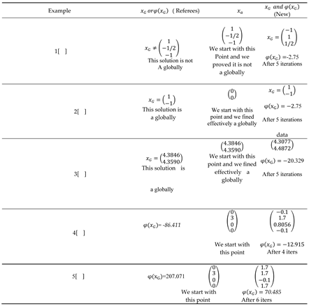
Our work is well justified by comparing it with some more recent methods with benchmarks used in the literature [7,13,14,15,16]. We note that the researchers left this track for a long time by used the Inertia-Controlling method, although with a small modification of this method, we managed to find good results.
In addition to the simplicity for verifying the global optimality conditions, the results have also been improved. In the concave case (Table 4).
However, in the indefinite case (Table 3) and convex cases (Table 2), our results are obtained with a minimal number of iterations and the determined solution is very better, which confirms the originality of our solving technique.
The results have also been improved. In the convex case (Table 1: Data for Convex Case Examples and Table 2: Results for Convex Case Examples). However, in the concave case (Table 3: Data for Concave Case
Examples and Table 4: results for Concave Case Examples) and indefinite case (Table 5: Data for Indefinite Case Examples and Table 6: Results for Indefinite Case Examples), our results are obtained with a minimal number of iterations and the determined solution is very better, which confirms the originality of our solving technique. 1-Convex case Results by using Path Method with Weight ( P.M.W. ) with depart point . New Results with the same initial or depart point .
Table 2.
Data for Convex Case Examples.
| Example A | H | B | c |
| 1 [] | |||
| 2 [] | |||
| 3 [] | |||
Table 3.
Results for Convex Case Examples.
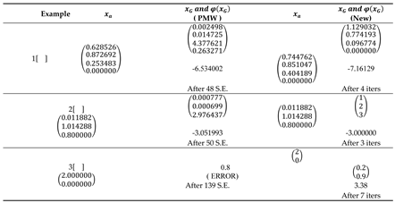 |
Table 4.
Data for Concave Case Examples.
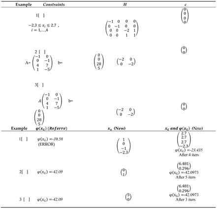 |
Table 5.
Data for Indefinite Case Examples.
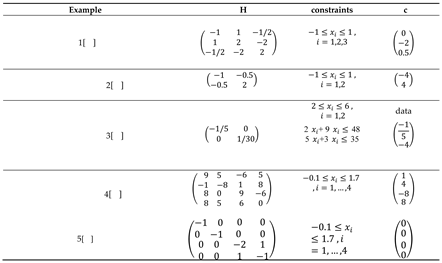 |
Table 6.
Results for Indefinite Case Examples.
 |
8. Conclusion
In this article we have shown that it is possible to check the global optimization conditions to decide that completed point of the Inertia-Controlling method (I.C.M.)is a global solution or not.
In the fact that any optimization problem is solved by the necessary and sufficiently conditions of its solutions, when these conditions are satisfied at the point denoted in our (P) problem by, this later becomes a solution to the considered problem.
However, if the relevant conditions are not found then we can’t obtain the exact solution.
Through these new sufficient conditions for global optimality we can apply any decreasing method converges to a local solution of problem (P) and we can also say that any point x of the field is a global solution of our mathematical problem or not, this is on the one hand.
On the other hand, the condition that we changed in this work depends on the solution of a linear system that is listed before in the local solution of objective function , and in our theories, the given direction q is a best decreasing of the objective functionatin terms of minimization, because all negative Eigen values of the matrix are taken, as we have also shown the decrease objective function at each active point in the convex, indefinite and singular case.
The results found provide high efficiency and reliability compared to the methods used (for example interior points) to resolve the quadratic programming problems at point of view of Accuracy and response times (a large number of iterations may be to find the solution).
Consequently, we recommend and ask that the method of I.C.M be seen again and used in many academic research which encourage university researchers to resort to this mathematical method to enrich their research in the scientific fields of applied mathematics and economics.
References
- Gill, P. E.; Murray, W.; Saunders, M. A. ; Wright, M. H., Inertia-controlling methods for general quadratic programming, SIAM Review, 1--36 (1991).
- Altman, A. ; Gondzio, J. Regularized symmetric indefinite systems in interior point methods for linear and quadratic optimi- zation, Optimization Methods and Software ; 1999;11(1-4), 275--302. [CrossRef]
- Grippo, L. ; Sciandrone, M..; Introduction to Interior Point Methods}, In Introduction to Methods for Nonlinear Optimiza- tion; 2023; pp.~497--527. Cham: Springer International Publishing. 346.
- Gondzio, J.; Sarkissian, R.;,Parallel interior-point solver for structured linear programs}, Mathematical Programming}, 2003; 96, 561—584.
- Fu, Y.; Liu, D.; Chen, J.; He, L.; Secretary bird optimization algorithm: a new metaheuristic for solving global optimization problems, Artificial Intelligence Review, 2024; 57(5), 123.
- Kim, S.; Kojima, M.; Equivalent sufficient conditions for global optimality of quadratically constrained quadratic programs, 351 Mathematical Methods of Operations Research, 2025; 101(1), 73--94.
- Kebbiche, Z. ; Etude et extensions d’algorithmes de points intérieurs pour la programmation non linéaire, Doctoral disser- 353 tation, Université de Sétif (2008).
- Azevedo, A. T.; Oliveira, A. R. L;.Soares, S.; Interior point method for long-term generation scheduling of large-scale hydro- 355 thermal systems,Annals of Operations Research, 2009; 169(1),55--80.
- Morales, J. L.; Nocedal, J. ; Wu, Y.,A; sequential quadratic programming algorithm with an additional equality constrained 357 phase,IMA Journal of Numerical Analysis, 2012; 32(2), 553--579.
- Jose Pierre Dusqult,’ Programmation non linéaire’ ; université de sherbooke ; Département D’infor- 359 matique ; 110665970(2011).
- Gondzio, J, ; Yildrim, E. A.; Global solutions of nonconvex standard quadratic programs via mixed integer linear program- 361 ming reformulations, Journal of Global Optimization, 2021; {81}(2), 293--321. [CrossRef]
- Pedregal, P.; Introduction to Optimization, 2004; Vol. 46. New York: Springer. [CrossRef]
- Choufi, S.; Development of a procedure for finding active points of linear constraints, Journal of Applied and Computational 365 Mathematics, 2017; 6(2).
- Sun, W.; Yuan, Y. X.; Optimization Theory and Methods: Nonlinear Programming, 2006; (Vol. 1).New York: Springer Sci- ence Business Media.
- Wu, Z. Y. ; Bai, F. S,; Global optimality conditions for mixed nonconvex quadratic programs,Optimization, 2009; 58(1), 39-- 369 47.
- Sun, X. L.; Li, D. ; McKinnon, K. I. M..; On saddle points of augmented Lagrangians for constrained nonconvex optimiza- 371 tion,SIAM Journal on Optimization, 2005; 12(4), 1128--1146.
- Messine, F. ; Jourdan N. ; L’optimisation globale par intervalles: de l’étude théorique aux applications, Habilitation à Diriger des Recherches, Institut National Polytechnique de Toulouse ,2006.
- Morales, J. L..; Nocedal, J. ; Wu, Y.,A.; sequential quadratic programming algorithm with an additional equality constrained phase,IMA Journal of Numerical Analysis, 2012; 32(2), 553--579.
- Huang, W.; Zou, J.; Liu, Y.; Yang, S.. ; Zheng, J.; Global and local feasible solution search for solving constrained multi- 377 objective optimization, Information Sciences, 2023; 649, 119467.
- Kim, S. ; Kojima, M.; Equivalent sufficient conditions for global optimality of quadratically constrained quadratic programs, Mathematical Methods of Operations Research, 2025; 101(1), 73--94.
- Ouaoua, M. L. ; Khelladi, S.; Efficient Descent Direction of a Conjugate Gradient Algorithm for Nonlinear Optimization, 381 Nonlinear Dynamics and Systems Theory, 2025; 25(1), XXX--XXX.
Disclaimer/Publisher’s Note: The statements, opinions and data contained in all publications are solely those of the individual author(s) and contributor(s) and not of MDPI and/or the editor(s). MDPI and/or the editor(s) disclaim responsibility for any injury to people or property resulting from any ideas, methods, instructions or products referred to in the content. |
© 2025 by the authors. Licensee MDPI, Basel, Switzerland. This article is an open access article distributed under the terms and conditions of the Creative Commons Attribution (CC BY) license (http://creativecommons.org/licenses/by/4.0/).
Copyright: This open access article is published under a Creative Commons CC BY 4.0 license, which permit the free download, distribution, and reuse, provided that the author and preprint are cited in any reuse.


