Submitted:
14 May 2025
Posted:
15 May 2025
You are already at the latest version
Abstract
In this paper, we propose a novel alternating direction method of multipliers based on inertial acceleration techniques for a class of nonconvex optimization problems with a two-block structure. To address the nonconvex subproblem, we introduce a proximal term to reduce the difficulty of solving this subproblem. For smooth subproblem, we employ a gradient descent method on the augmented Lagrangian function, which significantly reduces the computational complexity. Under the assumptions that the generated sequence is bounded and the auxiliary function satisfies Kurdyka-\L{ojasiewicz} property, we establish the global convergence of the proposed algorithm. Finally, the effectiveness and superior performance of the proposed algorithm are validated through numerical experiments in signal processing and SCAD problems.
Keywords:
convergence analysis
; nonconvex optimization
; alternating direction method of multipliers
; inertial term
; Kurdyka-Lojasiewicz inequality
MSC: 90C26; 65K05; 49K35; 41A25
1. Introduction
In recent years, nonconvex optimization problems have found widespread applications in science and engineering. For instance, Mohammadreza et al. [1] investigated the optimization of local nonconvex objective functions in time-varying networks based on the gradient tracking algorithm. And then, the researchers had explored optimizing nonconvex objective functions in multi-node networks under imperfect data exchange links. Zhang et al. [2] pointed out that traditional optimization methods often lead to target feature compression and information loss in motor imagery decoding, thereby reducing classification performance. Further, to address the high dimensionality and small sample size characteristics of motor imagery signals, Zhang et al. [2] proposed a nonconvex sparse regularization model constructed using the Cauchy function. This approach enables more accurate extraction of target features across multiple datasets while effectively suppressing noise interference. In addition, Tiddeman and Ghahremani [3] combined wavelet transforms with principal component analysis to propose a class of principal component waveform networks for solving linear inverse problems, they fully utilized the symmetry in wavelet transforms during the wavelet decomposition, ensuring the effectiveness of image reconstruction. For more related works, one can see [4,5,6] and the references therein.
It is well known that recovering sparse signals from incomplete observations is an important research direction in practical applications. The core objective is to find the optimal sparse solution to a system of linear equations, which can be formulated as the following model [7]:
where A is the measurement matrix, b is the observed data, x is a sparse signal, is a regularization parameter, and denotes the -norm. However, Chartrand and Staneva [8] pointed out that the above problem represents a class of problems that are fundamentally difficult to solve. To overcome this challenge, Zeng et al. [9] proposed a relaxed objective function by replacing the regularization with the regularization, the problem is transformed into a more tractable nonconvex optimization problem. Therefore, adopting this modification becomes more reasonable in signal recovery problems, which leads to the following two-block nonconvex optimization problem:
where . In general, we would consider introducing an auxiliary variable y to reformulate the problem (1) as follows
Zeng et al. [9] pointed out that the iterative soft-thresholding algorithm can be used to solve the regularization problem, which was validated in context of problem (2). Meanwhile, Chen and Selesnick [10] performed a performance validation of model (2) using an improved overlapping shrinkage algorithm. In addition, further related works can be found in [11,12].
In statistical optimization, certain penalty methods exhibit limitations, such as vulnerability to data circumvention and biased estimation of significant variables [14]. To address these issues, Fan and Li [14] proposed the smoothly clipped absolute deviation (SCAD) penalty function. They developed optimization algorithms to solve non-concave penalized likelihood problems and demonstrated that this method possesses asymptotic oracle properties. Remarkably, with appropriate regularization parameter selection, the results can achieve nearly identical performance to the known true model. SCAD penalty problem proposed by scholars can be conceptually understood as
with , , and the penalty function in the objective, we refer readers to (26) later. As shown above, problems of the forms (2) and (3) can be generalized to the following nonconvex optimization problem:
where f is a lower semicontinuous function from to , and is a differentiable function whose gradient is L-Lipschitz continuous with . Here, A denotes a matrix in , and . Variants of model (4) have found applications in various fields, such as statistical learning [15,16,17], penalized zero-variance discriminant analysis [18] and image reconstruction [19,20].
It is well known that the alternating direction method of multipliers (ADMM) has gained widespread attention due to its balance between performance and efficiency. When the subproblems are independent, ADMM exhibits a unique symmetry. In fact, with appropriately designed update steps, this symmetry ensures that the convergence of ADMM is independent of the order in which the subproblems are updated [21]. In recent years, as nonconvex optimization problems have gained increasing attention, the convergence analysis of ADMM in nonconvex settings has become a research hotspot. Hong et al. [22], recognizing the strong empirical performance of ADMM on nonconvex problems but the lack of theoretical guarantees, not only established the convergence theory for nonconvex ADMM but also overcame the limitation on the number of variable blocks. Wang et al. [23] demonstrated that incorporating the Bregman distance into ADMM can effectively simplify the computation of subproblems, emphasizing the feasibility of ADMM in nonconvex settings. Ding et al. [24] proposed a class of Semi-Proximal ADMM for solving low-rank matrix recovery problems. In the presence of noisy matrix data, by minimizing the nuclear norm, they effectively addressed the issues of Gaussian noise and related mixed noise. Guo et al. [25] provided insights into solving large-scale nonconvex optimization problems using ADMM. For more related work, readers may refer to [26,27,28,29].
The inertial acceleration technique, derived from the heavy-ball method, utilizes information from previous iterations to construct affine combinations [30]. Additionally, we observe that inertial techniques can employ different extrapolation strategies during the optimization process to enhance convergence speed. In their study of the general inertial proximal gradient method, Wu and Li [31] proposed two distinct extrapolation strategies to flexibly adjust the algorithm’s convergence rate. Chen et al. [32] investigated an inertial proximal ADMM and established the global convergence of iterates under appropriate assumptions. In fact, Chao et al. [33] also discovered that embedding the inertial term into the y-subproblem can significantly improve the algorithm’s convergence speed. Moreover, compared to the standard inertial update step , Wang et al. [34] considered a different update scheme, . This update step not only preserves the acceleration effect of inertia but also reduces computational errors introduced by the inertial term updates.
Unfortunately, the work of Wang et al. only considered the inertial update step for x. Inspired by the work in [34], we propose a novel symmetrical inertial alternating direction method of multipliers with proximal term (NIP-ADMM). Building upon Wang et al.’s inertial update step, we introduce an additional inertial update for y and incorporate into the x-subproblem update, this form of inertial update ensures that the primal variables are treated equally, thereby achieving faster acceleration. To simplify the computation of the subproblems, we introduce an approximation term in the x-subproblem, which under certain conditions, allows the nonconvex subproblem to be transformed into an approximate projection-type problem. Furthermore, since is convex, this property ensures that is well-defined, this enables us to abandon the traditional ADMM update scheme and instead adopt a gradient descent approach. This method requires only the computation of gradients at each iteration, significantly reducing computational complexity. Consequently, it offers substantial advantages when handling high-dimensional or large-scale datasets.
The structure of this paper is as follows. In Section 2, we review essential results required for further analysis. We present NIP-ADMM and analyze its convergence in Section 3. Numerical experiment and application to signal recovery in Section 4 highlight the benefits of the majorization and inertial techniques. Lastly, in Section 5, we sent a conclusion.
2. Preliminaries
In this section, we introduce key notations and definitions that are essential for the results to be developed and are utilized in the subsequent sections.
Assume , . If matrix Q is a positive definite (semi-definite positive) matrix, then we have . Given any matrix and a vector , let be Q-norm of x. For the matrix G, we define and as the smallest and largest eigenvalues of , respectively. If we denote , then the domain of the function is defined as .
Definition 1.
Let . Then the distance from point to S is defined as . In particular, if , then .
Definition 2.
For a differentiable convex function , the Bregman distance is defined by
where .
Definition 3.
Assume is a proper lower semicontinuous function.
- (i)
-
The Frechet sub-differential of f at is denoted by and defined as:Among others, we set when .
- (ii)
- The limiting sub-differential of f at is written as and defined by
Proposition 1.
The sub-differential of a lower semicontinuous function f possesses several fundamental and significant properties as follows:
- (i)
- From Definition 3, which implies that holds for all , and given that is a closed set, is also a closed set.
- (ii)
- Suppose that is a sequence that converges to , and converges to with . Then, by the definition of the sub-differential, we have .
- (iii)
- If is a local minimum of f, then it follows that .
- (vi)
- Assuming that is a continuously differentiable function, we can derive:
Definition 4.
We consider the point to be a critical point of the augmented Lagrangian function if it satisfies the following conditions:
Definition 5
([36]). (Kurdyka-Łojasiewicz property (KLP)) Let be a proper lower semicontinuous function. For (), if there exists , a neighborhood U of , and a function , here is the set of the concave function , then for any , the following inequality holds
and we call that f satisfies KLP.
Lemma 1
([35]). Suppose that the matrix is a non-zero matrix, and let denote the smallest positive eigenvalue of the matrix . Then for each , the following holds:
Lemma 2
([36]). Assume , where and are both proper lower semicontinuous functions. Then, for any , we can obtain
Lemma 3
([37]). (Uniformized KLP) Let Ω be a compact set and be the same as in Definition 5. If a proper lower semicontinuous function is fixed at a point in Ω and satisfies the KLP at every point on Ω, and there exist , , and such that for any and , then the following inequality is satisfied:
Lemma 4
([38]). If the function is continuously differentiable, and is Lipschitz continuous with constant , then for any , the following result holds:
3. Algorithm and Convergence Analysis
In this section, we first present the definition of the augmented Lagrangian function associated with problem (4) as follows:
where denotes the augmented Lagrange multiplier, and is a penalty parameter. Following this, we propose the NIP-ADMM for solving the problem (4), the proposed algorithm is outlined below:
Remark 1.
- (i)
- In NIP-ADMM, the inertial parameters η and θ are both in , and S is a positive semi-definite matrix.
- (ii)
- The update scheme for the y-subproblem adopts the gradient descent method, where is the gradient of the function L with respect to y, and γ is called the learning rate.
- (iii)
- The inertial structure we adopted employs a structurally balanced acceleration strategy. This update strategy is mathematically symmetric, with the only distinction being the values of the parameters η and θ.
According to Algorithm 1, the optimality conditions for NIP-ADMM are obtained as
Before concluding this section, we present the following fundamental assumptions, which are essential for the convergence analysis.
| Algorithm 1: NIP-ADMM |
|
Initialization: Input , and , let , and . Given constants . Set .
While "not converge" Do Compute . Execute to determine . Calculate . Update dual variable . Let . End While Output: output of the problem (4). |
Assumption 1. (i) is a proper lower semicontinuous function. is continuously differentiable, and is Lipschitz continuous with a Lipschitz constant .
- (ii)
- S is a positive semidefinite matrix.
- (iii)
- For convenience, we introduce the following symbols:
- (iv)
- To analyze the monotonicity of , we set .
Lemma 5.
If Assumption 1 holds, for any , then
where is the inertial parameter in Algorithm 1.
Proof.
According to the definition of the Lagrangian function, one gets
and we also can know that
Combining the above two formulas, one can declare
Since is the optimal solution to the subproblem with respect to x, one knows that
Noticing Algorithm 1 and (6), one can see
Thus, it is natural to derive the following process:
Combining (8) and Equations (10)–(12), one can draw the following conclusions:
where and , and we obtain the desired conclusion. □
According to Assumption 1 with and , the monotonic non-increasing property of the sequence is guaranteed.
Lemma 6.
If the sequence generated by the algorithm is bounded, then we have
Proof.
Since is bounded, it is evident that is also bounded. Moreover, there exists an accumulation point, let us assume it to be , and there exists a subsequence of such that
which implies that is bounded from below. From Lemma 5 and the condition , it follows that
Given , , and S is a positive semi-definite matrix, it is evident that one can derive that
By the inertial relationship, the following conclusion can be obtained:
Now we give subsequential convergence analysis of NIP-ADMM.
Theorem 1. (Subsequential Convergence) The sequence generated by NIP-ADMM is bounded, and assume S and are the sets of cluster points of and , respectively. Under the assumptions and the conditions of Lemma 5, we have the following conclusion:
- (i)
- M and are two non-empty compact sets. As , it follows that and .
- (ii)
- .
- (iii)
- .
- (iv)
- The sequence converges, and .
Proof.
- (i)
- Based on the definitions of M and , the conclusion can be satisfied.
- (ii)
- Combining Lemma 5 with the definitions of and , we obtain the desired conclusion.
- (iii)
-
Let , then we obtain that a subsequence of can converge to . By combining Lemma 5, as , one has , which implies . On one hand, noting that is the optimal solution to the x-subproblem, we haveFrom Lemma 6, we know that , and combining this with , we conclude that the equality holds. On the other hand, since is a lower semi-continuous function, we deduce that , so one getsMoreover, given the closedness of and the continuity of , along with and the optimality condition of NIP-ADMM (6), we assert thatand as established in Definition 4.
- (v)
-
Let , and assume that there exists a subsequence of that converges to . Combining the relations (14), (19), and the continuity of g, we haveConsidering that is monotonically non-increasing, it follows that is convergent. Consequently, for any , the relationship can be established as
□
Based on the definition of the augmented Lagrangian function and the semidefiniteness of the matrix S, the following can be defined with :
Then, the following result can be obtained.
Lemma 7.
Let be contained in . Then, there exists and such that
Proof.
By the definition of and , we can derive that
Combining the above expression with the optimality conditions of NIP-ADMM (6), which means
It is easy to see from Lemma 2 that . Moreover, since has a Lipschitz continuous gradient with respect to L, we get
therefore, according to (20), there exists a positive real number such that
Furthermore, combining this with (12), we know that there exists and such that:
thus, by selecting and , we can further conclude that
this concludes the proof. □
Theorem 2. (Global convergence) Suppose the sequence generated by NIP-ADMM is bounded, and the assumptions hold. If is a KL function, then
Moreover, the sequence converges to a critical point of .
Proof.
From Theorem 1, we know that . For any , the proof process needs to consider the following two cases:
- (i)
-
For any and given that , it follows from Lemma 1 and Lemma 5 that there exists a constant such that
- (ii)
-
Assume that for any , the inequality holds. Sinceit follows that for any , there exists such that for all , we have:Moreover, noting thatit implies that for any , there exists such that for all , the inequality holds:Hence, given and , when , we haveAnd, based on Lemma 3, the following holds for all , it can be deduced thatFurthermore, using the concavity of , we derive the following:Noting the fact that , together with the conclusion obtained in Lemma 7, we can infer thatwhere represents and represents Combining Lemma 5, we can rewrite (22) as followswhere (22) can be equivalently expressed asBy applying the Cauchy-Schwarz inequality and multiplying both sides by 6, we obtainThen, by further applying the fundamental inequality, we can deduce thatNext, summing up (23) from to and rearranging the terms, one getsFurthermore, as and m approaches positive infinity, we can conclude thatwhich impliesThis demonstrates that forms a Cauchy sequence, which ensures its convergence. By applying Theorem 1, it follows that converges to a critical point of .
□
4. Numerical Simulations
In this section, we demonstrate the application of NIP-ADMM in signal recovery and SCAD penalty problems. To verify the effectiveness of the algorithm, we compare it with Bregman modification of ADMM (BADMM) proposed by Wang et al. [23] and inertial proximal ADMM (IPADMM) proposed by Pi et al. [32]. All codes were implemented in MATLAB 2024b and executed on a Windows 11 system equipped with an AMD Ryzen R9-9900X CPU.
4.1. Signal Recovery
In this subsection on signal recovery, we consider the previously mentioned model (2).
where , and ,, . To evaluate the effectiveness of NIP-ADMM, we compare it with BADMM [23] and IPADMM [32]. We construct the following framework to solve problem (24). We set , where I denotes the identity matrix.
Here, represents the half-shrinkage operator proposed by Xu et al. [39], which is defined as
where the function for is defined by
In this setup, the entries of matrix A are drawn from a standard normal distribution, with each column adjusted for normalization. The starting vector is initialized as a sparse vector, containing at least 100 non-zero components. The values are set initially to zero. To simulate the observation vector with added noise, we generate b using , where . For the regularization parameter c, we compute
Based on Assumption 1, the parameters are chosen as and . The error trend is depicted as At the -th iteration, the primal residual is expressed as while the Dual residual is represented as Termination occurs when both conditions are met: and During the experiments, to satisfy Assumption 1, we set . Table 1 shows that when , selecting the inertial parameter values and produces satisfactory results. Therefore, in subsequent experiments, we also adopt and . The metrics include the number of iterations (Iter), CPU running time (CPUT) and the objective function value (Obj). To better present the experimental results, we retain two decimal places for Obj and four decimal places for CPUT.
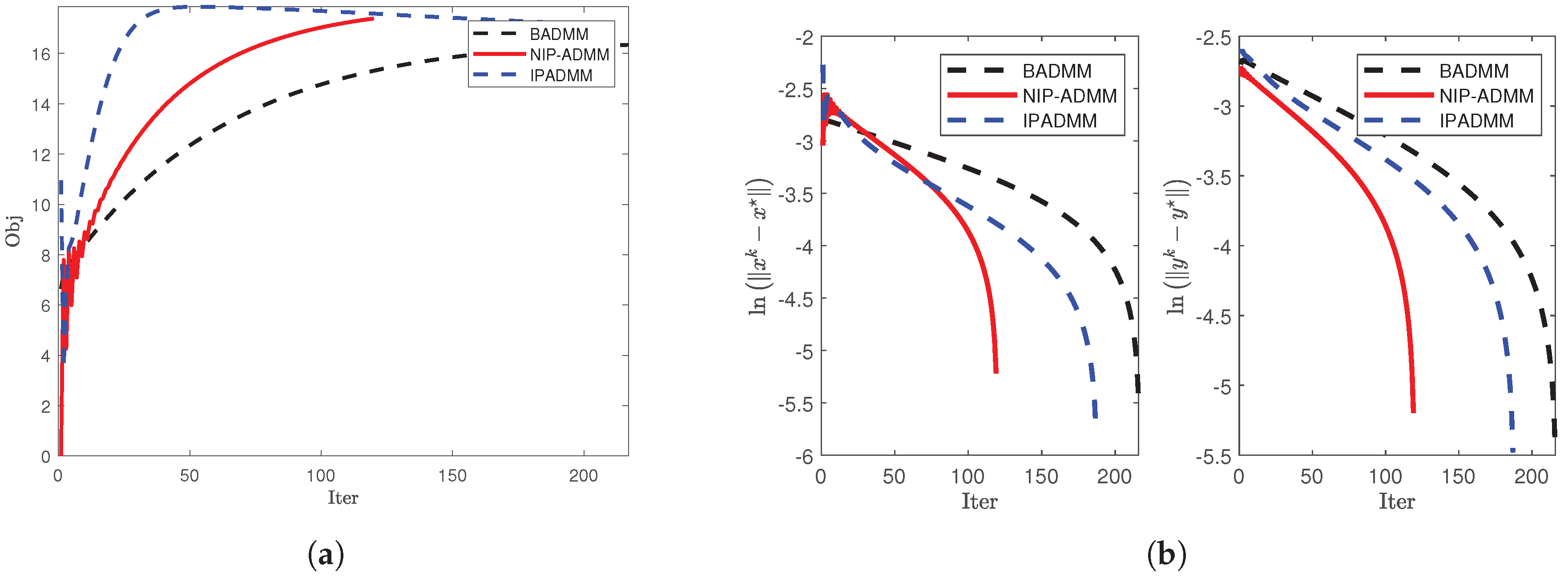
The numerical results consistently demonstrate the superior performance of NIP-ADMM compared to BADMM and IPADMM (see Table 2): for , NIP-ADMM shows faster convergence in terms of both objective value and error reduction (see Figure 1); for and , the inclusion of the inertial term further highlights its effectiveness (see Figure 2); and for larger-scale models with , it is proven that NIP-ADMM is more suitable than BADMM and IPADMM for handling large-scale problems (see Figure 3).
4.2. SCAD Penalty Problem
We note that the smoothly clipped absolute deviation (SCAD) penalty problem in statistics can be formulated as the following model [14,31]:
with ,, and the penalty function in the objective is defined as:
where and , being the knots of the quadratic spline function. In the reference signal recovery subsection, we similarly set and , where . For the problem (25), the x-subproblem can be expressed as
On the one hand, the x-subproblem can be equivalently formulated as:
On the other hand, under the condition that , we can update x using the following rule [31]:
where represents the positive part operator, which is defined as , applying NIP-ADMM to solve the problem (25), one yields that
Similarly, the update scheme of BADMM can be represented by the following procedure:
Utilize the IPADMM to address model (25) and derive the following iterative scheme:
In this experiment, we generate a random matrix A, and perform row and column normalization. Here, we choose to generate a vector z of dimension n with a sparsity ratio of . The vector b is represented as the sum of and a Gaussian noise vector with zero mean and variance . The initial variables and are set as zero vectors, serving as the starting point for optimization. To improve numerical efficiency, in this experiment, we set and . Under the condition that Assumption 1 is satisfied, we configure , , and for NIP-ADMM and other algorithms. The stopping criterion for the updates is set as
In Table 3, we set . The results in the table support our choice of the inertial parameters and . Under these conditions, the NIP-ADMM requires the fewest iterations and the least running time. Therefore, we selected the inertial parameters and for the experiments.
To further investigate the convergence behavior of the algorithms, we plot the update curves of the objective function (left figure) and the iteration error (right figure) against the number of iterations for each algorithm under three different dimensions (see Figure 4, Figure 5, and Figure 6). The numerical results demonstrate that NIP-ADMM achieves nearly the same performance as IPADMM and BADMM but with significantly fewer iterations.
Figure 4.
Comparison of convergence when and : (a) The objective value when and . (b) and under .
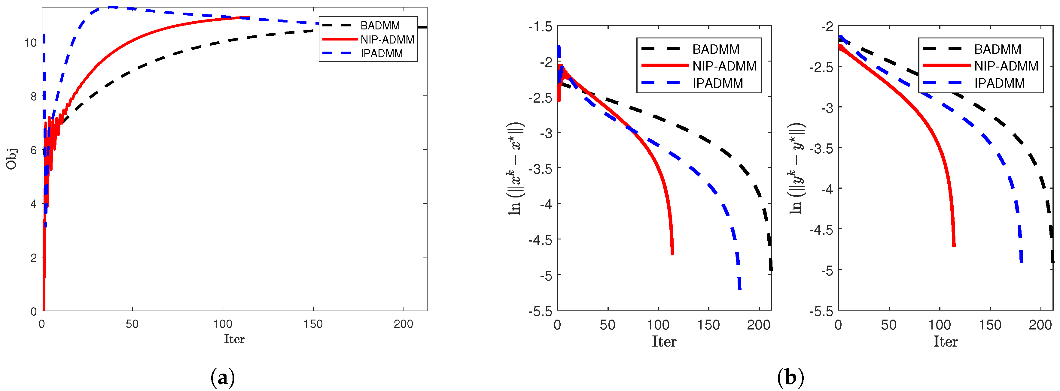
Figure 5.
Comparison of convergence when and : (a) The objective value when and . (b) and under .
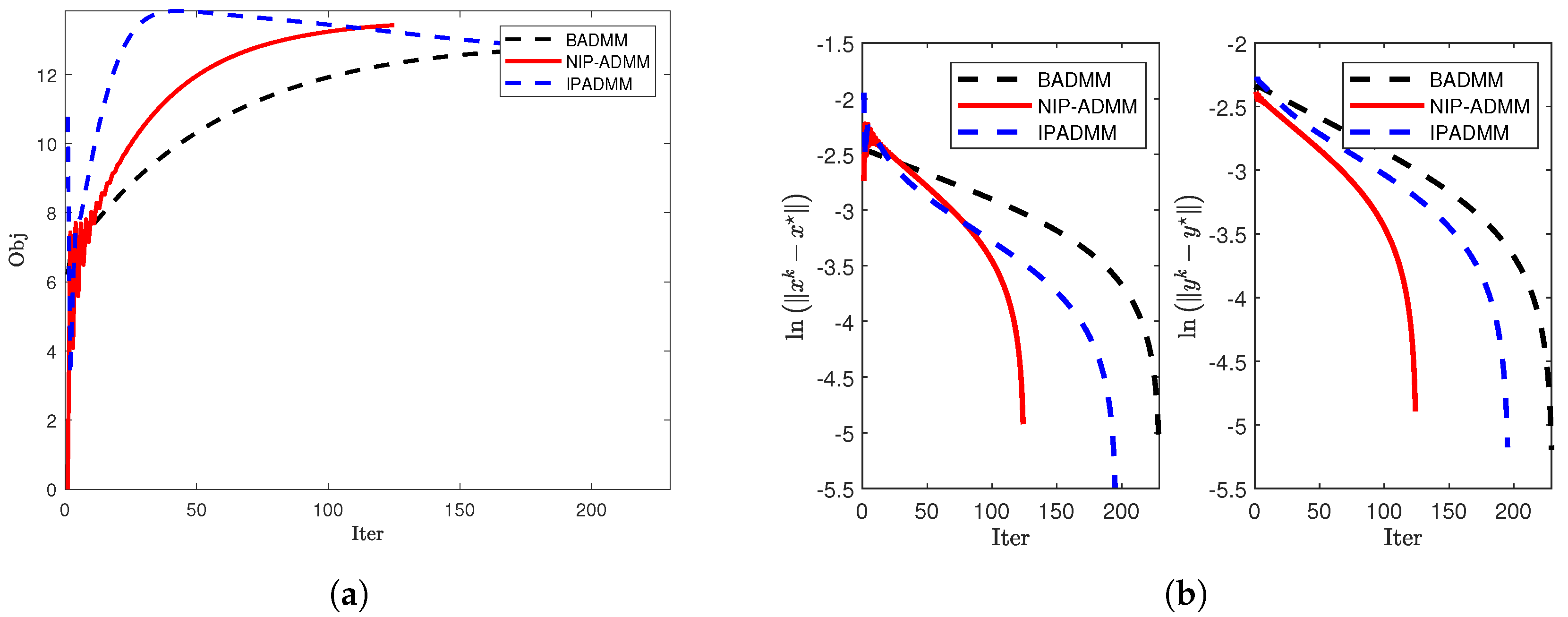
Figure 6.
Comparison of convergence when and : (a) The objective value when and . (b) and under .
In Table 4, we present the test results of NIP-ADMM, BADMM and IPADMM under different dimensions. Although there are slight discrepancies in the Obj values between the two methods, by focusing on the metrics of Iter and CPUT, it is evident that NIP-ADMM demonstrates a significant advantage over BADMM and IPADMM. This advantage becomes even more pronounced in higher-dimensional scenarios.
5. Conclusion
The Purpose of this is to propose a novel symmetrical inertial ADMM with proximal term for solving nonconvex two-block optimization problems. Under certain conditions, if the objective function satisfies Kurdyka-Łojasiewicz property, the sequence generated by the algorithm globally converges to a stationary point. In numerical experiments, we apply the algorithm to signal recovery and SCAD penalty problems, and its superiority is validated. Notably, by continuously adjusting the inertial parameters, we identify a set of parameters that enhances the convergence speed of the algorithm.
Furthermore, we believe that future work could explore whether the convergence of the algorithm can be guaranteed when the objective function is non-separable. Additionally, it would be worthwhile to investigate whether introducing inertial terms into the y-subproblem and the multiplier could further accelerate the convergence speed of the algorithm.
Author Contributions
Conceptualization, J.-h.L. and H.-y.L.; methodology, J.-h.L.; software, J.-h.L. and S.-y.L.; validation, J.-h.L. and H.-y.L.; writing—original draft preparation, J.-h.L. and H.-y.L.; writing—review and editing, J.-h.L. and H.-y.L.; visualization, J.-h.L, H.-y.L. and S.-y.L.; supervision, H.-y.L.; project administration, H.-y.L. All authors have read and agreed to the published version of the manuscript.
Funding
This research was funded by the Innovation Fund of Postgraduate, Sichuan University of Science & Engineering (Y2024340), the Scientific Research and Innovation Team Program of Sichuan University of Science and Engineering (SUSE652B002) and the Opening Project of Sichuan Province University Key Laboratory of Bridge Non-destruction Detecting and Engineering Computing (2023QZJ01).
Data Availability Statement
The raw data supporting the conclusions of this article will be made available by the authors on request.
Conflicts of Interest
The authors declare no conflicts of interest.
References
- Zhang, S.R.; Wang, Q.H.; Zhang, B.X.; Liang, Z.; Zhang, L.; Li, L.L.; Huang, G.; Zhang, Z.G.; Feng, B.; Yu, T.Y. Cauchy non-convex sparse feature selection method for the high-dimensional small-sample problem in motor imagery EEG decoding. Front. Neurosci. 2023, 17, 1292724. [Google Scholar] [CrossRef] [PubMed]
- Doostmohammadian, M.; Gabidullina, Z.R.; Rabiee, H.R. Nonlinear perturbation-based non-convex optimization over time-varying networks. IEEE Trans. Netw. Sci. Eng. 2024, 11, 6461–6469. [Google Scholar] [CrossRef]
- Tiddeman, B.; Ghahremani, M. Principal component wavelet networks for solving linear inverse problems. Symmetry. 2021, 13, 1083. [Google Scholar] [CrossRef]
- Xia, Z.C.; Liu, Y.; Hu, C.; Jiang, H.J. Distributed nonconvex optimization subject to globally coupled constraints via collaborative neurodynamic optimization. Neural Netw. 2025, 184, 107027. [Google Scholar] [CrossRef] [PubMed]
- Yu, G.; Fu, H.; Liu, Y.F. High-dimensional cost-constrained regression via nonconvex optimization. Technometrics. 2021, 64, 52–64. [Google Scholar] [CrossRef]
- Merzbacher, C.; Mac Aodha, O.; Oyarzún, D.A. Bayesian optimization for design of multiscale biological circuits. ACS Synth. Biol. 2023, 12, 2073–2082. [Google Scholar] [CrossRef] [PubMed]
- Kim, S.j.; Koh, K.; Lustig, M.; Boyd, S.; Gorinevsky, D. An interior-point method for large-scale ℓ1-regularized least Squares. IEEE J. Sel. Top. Signal Process. 2007, 1, 606–617. [Google Scholar] [CrossRef]
- Chartrand, R.; Staneva, V. Restricted isometry properties and nonconvex compressive sensing. Inverse Problems. 2008, 24, 035020. [Google Scholar] [CrossRef]
- Zeng, J.S.; Lin, S.B.; Wang, Y.; Xu, Z.B. L1/2 regularization: convergence of iterative half thresholding algorithm. IEEE Trans. Signal Process. 2014, 62, 2317–2329. [Google Scholar] [CrossRef]
- Chen, P.Y.; Selesnick, I.W. Group-sparse signal denoising: non-convex regularization, convex optimization. IEEE Trans. Signal Process. 2014, 62, 3464–3478. [Google Scholar] [CrossRef]
- Bai, Z.L. Sparse Bayesian learning for sparse signal recovery using ℓ1/2-norm. Appl. Acoust. 2023, 207, 109340. [Google Scholar] [CrossRef]
- Wang, C.; Yan, M.; Rahimi, Y.; Lou, Y.F. Accelerated schemes for the L1/L2 minimization. IEEE Trans. Signal Process. 2020, 68, 2660–2669. [Google Scholar] [CrossRef]
- Beck, A.; Teboulle, M. A fast iterative shrinkage-thresholding algorithm for linear inverse problems. SIAM J. Imaging Sci. 2009, 2, 183–202. [Google Scholar] [CrossRef]
- Fan, J.Q.; Li, R.Z. Variable selection via nonconcave penalized likelihood and its oracle properties. J. Amer. Statist. Assoc. 2001, 96, 1348–1360. [Google Scholar] [CrossRef]
- Bai, J.C.; Zhang, H.C.; Li, J.C. A parameterized proximal point algorithm for separable convex optimization. Optim. Lett. 2018, 12, 1589–1608. [Google Scholar] [CrossRef]
- Wen, F.; Liu, P.L.; Liu, Y.P.; Qiu, R.C.; Yu, W.X. Robust sparse recovery in impulsive noise via ℓp-ℓ1 optimization. IEEE Trans. Signal Process. 2017, 65, 105–118. [Google Scholar] [CrossRef]
- Zhang, H.M.; Gao, J.B.; Qian, J.J.; Yang, J.; Xu, C.Y.; Zhang, B. Linear regression problem relaxations solved by nonconvex ADMM with convergence analysis. IEEE Trans. Circuits Syst. Video Technol. 2023, 34, 828–838. [Google Scholar] [CrossRef]
- Ames, B.P.W.; Hong, M.Y. Alternating direction method of multipliers for penalized zero-variance discriminant analysis. Comput. Optim. Appl. 2016, 64, 725–754. [Google Scholar] [CrossRef]
- Zietlow, C.; Lindner, J.K.N. ADMM-TGV image restoration for scientific applications with unbiased parameter choice. Numer. Algorithms. 2024, 97, 1481–1512. [Google Scholar] [CrossRef]
- Bian, F.M.; Liang, J.W.; Zhang, X.Q. A stochastic alternating direction method of multipliers for non-smooth and non-convex optimization. Inverse Problems. 2021, 37, 075009. [Google Scholar] [CrossRef]
- Parikh, N.; Boyd, S. Proximal Algorithms; Now Publishers: Braintree, MA, USA, 2014. [Google Scholar]
- Hong, M.Y.; Luo, Z.Q.; Razaviyayn, M. Convergence analysis of alternating direction method of multipliers for a family of nonconvex problems. SIAM J. Optim. 2016, 26, 337–364. [Google Scholar] [CrossRef]
- Wang, F.H.; Xu, Z.B.; Xu, H.K. Convergence of Bregman alternating direction method with multipliers for nonconvex composite problems. arXiv 2014, arXiv:1410.8625. [Google Scholar]
- Ding, W.; Shang, Y.; Jin, Z.; Fan, Y. Semi-proximal ADMM for primal and dual robust Low-Rank matrix restoration from corrupted observations. Symmetry. 2024, 16, 303. [Google Scholar] [CrossRef]
- Guo, K.; Han, D.R.; Wu, T.T. Convergence of alternating direction method for minimizing sum of two nonconvex functions with linear constraints. Int. J. Comput. Math. 2016, 94, 1653–1669. [Google Scholar] [CrossRef]
- Wang, Y.; Yin, W.T.; Zeng, J.S. Global convergence of ADMM in nonconvex nonsmooth optimization. J. Sci. Comput. 2019, 78, 29–63. [Google Scholar] [CrossRef]
- Wang, F.H.; Cao, W.F.; Xu, Z.B. Convergence of multi-block Bregman ADMM for nonconvex composite problems. Sci. China Inf. Sci. 2018, 61, 122101. [Google Scholar] [CrossRef]
- Barber, R.F.; Sidky, E.Y. Convergence for nonconvex ADMM, with applications to CT imaging. J. Mach. Learn. Res. 2024, 25, 1–46. [Google Scholar] [PubMed]
- Wang, X.F.; Yan, J.C.; Jin, B.; Li, W.H. Distributed and parallel ADMM for structured nonconvex optimization problem. IEEE Trans. Cybern. 2021, 51, 4540–4552. [Google Scholar] [CrossRef] [PubMed]
- Alvarez, F.; Attouch, H. An inertial proximal method for maximal monotone operators via discretization of a nonlinear oscillator with damping. Set-Valued Anal. 2001, 9, 3–11. [Google Scholar] [CrossRef]
- Wu, Z.M.; Li, M. General inertial proximal gradient method for a class of nonconvex nonsmooth optimization problems. Comput. Optim. Appl. 2019, 73, 129–158. [Google Scholar] [CrossRef]
- Chen, C.H.; Chan, R.H.; Ma, S.Q.; Yang, J.F. Inertial proximal ADMM for linearly constrained separable convex optimization. SIAM J. Imaging Sci. 2015, 8, 2239–2267. [Google Scholar] [CrossRef]
- Chao, M.T.; Zhang, Y.; Jian, J.B. An inertial proximal alternating direction method of multipliers for nonconvex optimization. Int. J. Comput. Math. 2020, 98, 1199–1217. [Google Scholar] [CrossRef]
- Wang, X.Q.; Shao, H.; Liu, P.J.; Wu, T. An inertial proximal partially symmetric ADMM-based algorithm for linearly constrained multi-block nonconvex optimization problems with applications. J. Comput. Appl. Math. 2023, 420, 114821. [Google Scholar] [CrossRef]
- Gonçalves, M.L.N.; Melo, J.G.; Monteiro, R.D.C. Convergence rate bounds for a proximal ADMM with over-relaxation stepsize parameter for solving nonconvex linearly constrained problems. arXiv 2017, arXiv:1702.01850. [Google Scholar]
- Attouch, H.; Bolte, J.; Redont, P.; Soubeyran, A. Proximal alternating minimization and projection methods for nonconvex problems: An approach based on the Kurdyka-Łojasiewicz inequality. Math. Oper. Res. 2010, 35, 438–457. [Google Scholar] [CrossRef]
- Bolte, J.; Sabach, S.; Teboulle, M. Proximal alternating linearized minimization for nonconvex and nonsmooth problems. Math. Program. 2014, 146, 459–494. [Google Scholar] [CrossRef]
- Nesterov, Y. Introductory Lectures on Convex Optimization: A Basic Course; Springer: NY, USA, 2004. [Google Scholar]
- Xu, Z.B.; Chang, X.Y.; Xu, F.M.; Zhang, H. L1/2 regularization: A thresholding representation theory and a fast solver. IEEE Trans. Neural Netw. Learn. Syst. 2012, 23, 1013–1027. [Google Scholar] [CrossRef] [PubMed]
Figure 1.
Comparison of convergence when and : (a) The objective value when and . (b) and under .
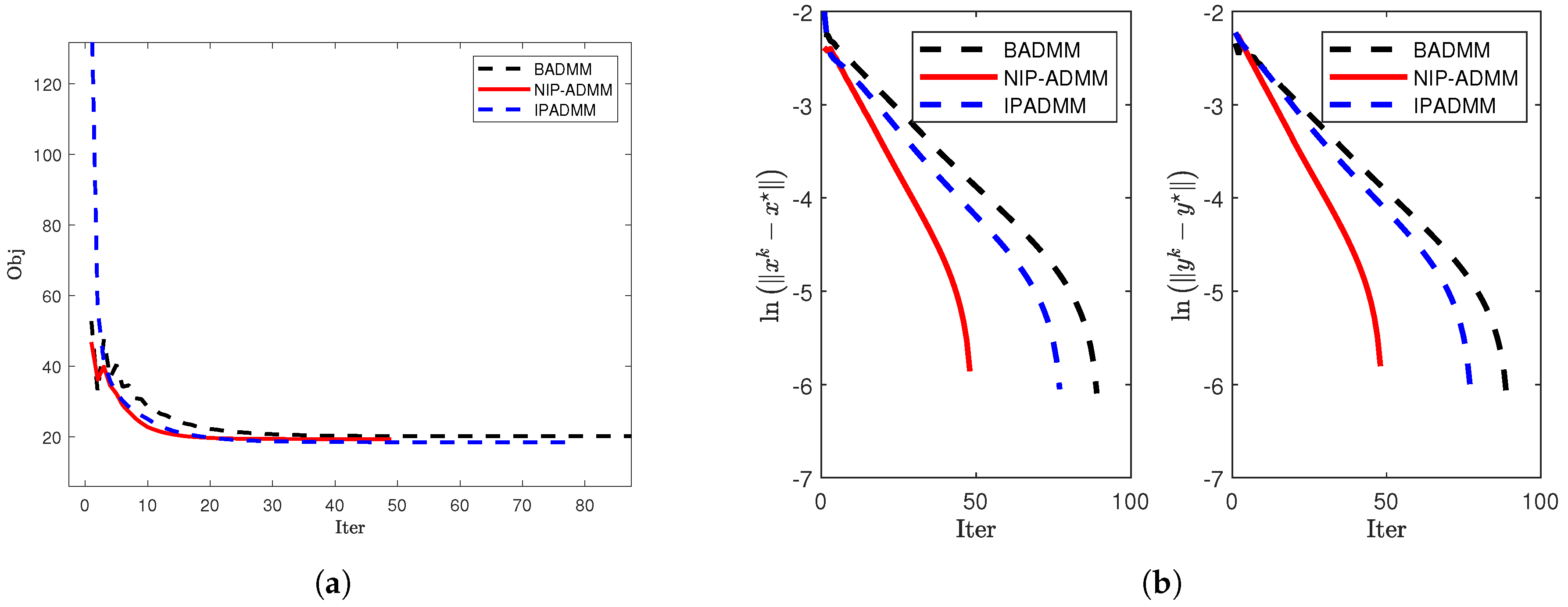
Figure 2.
Comparison of convergence when and : (a) The objective value when and . (b) and under .
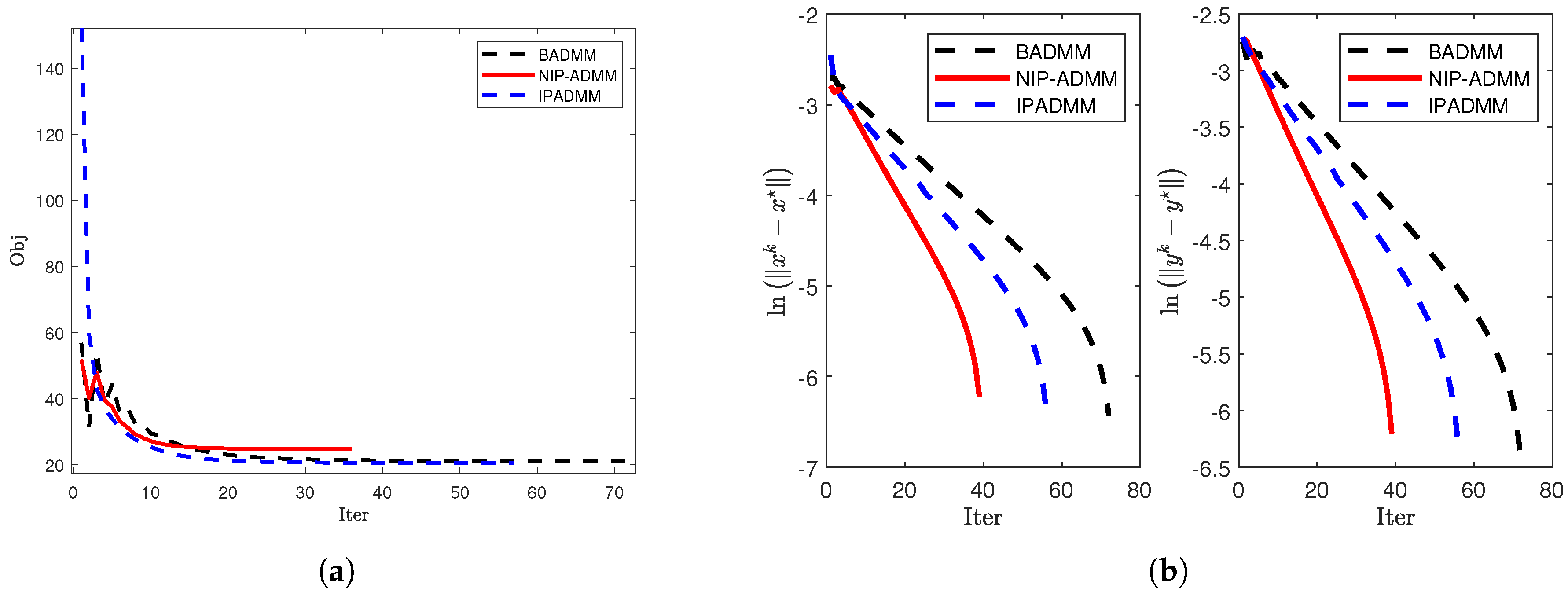
Figure 3.
Comparison of convergence when and : (a) The objective value when and . (b) and under .
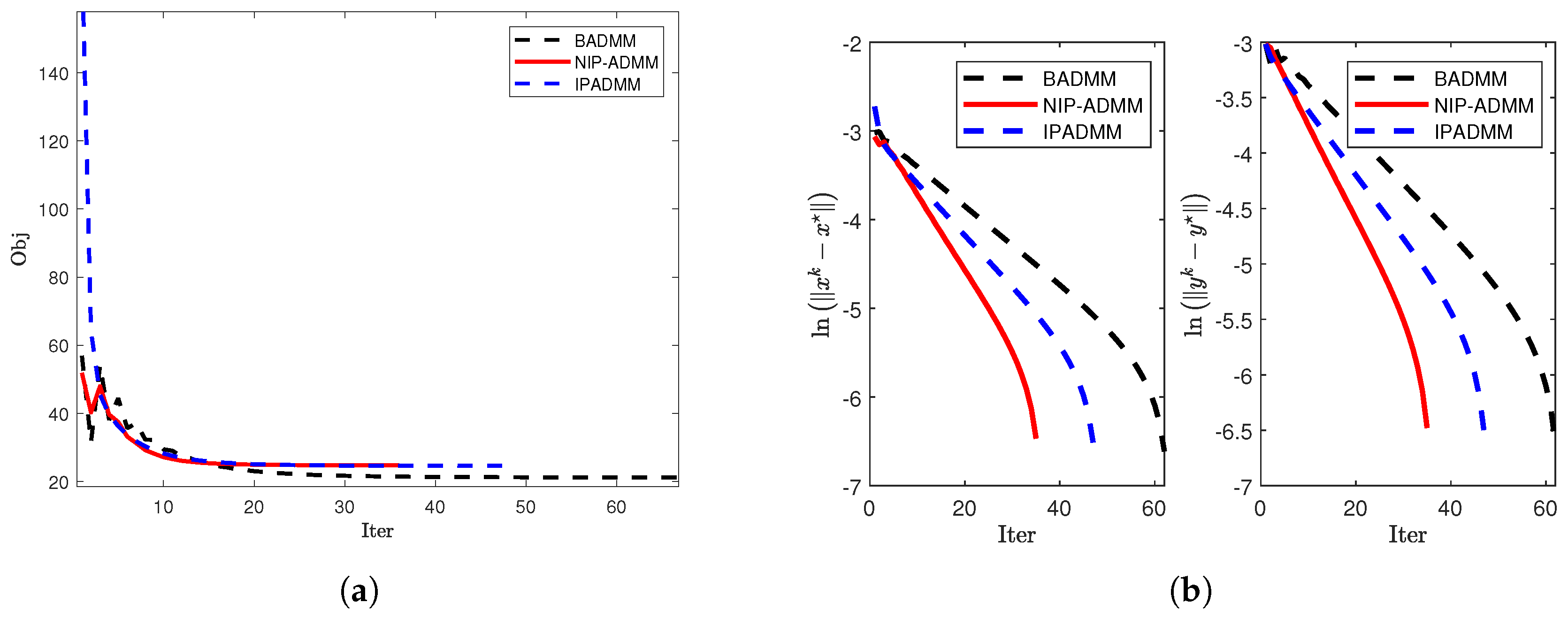

Table 1.
This is a table caption. Tables should be placed in the main text near to the first time they are cited.
Table 1.
This is a table caption. Tables should be placed in the main text near to the first time they are cited.
| Iter | CPUT(s) | Iter | CPUT(s) | ||||
|---|---|---|---|---|---|---|---|
| 0.2 | 0.2 | 75 | 2.2392 | 0.6 | 0.7 | 54 | 1.6014 |
| 0.3 | 0.2 | 78 | 2.3039 | 0.8 | 0.8 | 49 | 1.4583 |
| 0.3 | 0.3 | 69 | 1.9476 | 0.8 | 0.75 | 49 | 1.4309 |
| 0.5 | 0.5 | 60 | 1.7622 | 0.85 | 0.85 | 56 | 1.6445 |
| 0.6 | 0.6 | 56 | 1.6516 | 0.9 | 0.9 | 84 | 2.4614 |
Table 2.
Comparison of iteration effect between NIP-ADMM, IPADMM and BADMM.
| m | n | NIP-ADMM | IPADMM | BADMM | ||||||
|---|---|---|---|---|---|---|---|---|---|---|
| Iter | CPUT(s) | Obj | Iter | CPUT(s) | Obj | Iter | CPUT(s) | Obj | ||
| 1000 | 1000 | 49 | 1.2698 | 19.36 | 78 | 2.1407 | 18.46 | 90 | 2.3407 | 20.14 |
| 1500 | 2000 | 44 | 4.9152 | 23.17 | 72 | 8.4978 | 22.12 | 76 | 8.5387 | 23.69 |
| 3000 | 3000 | 40 | 15.0464 | 21.02 | 57 | 22.3823 | 20.56 | 73 | 27.4115 | 21.18 |
| 3000 | 4000 | 55 | 34.0601 | 23.21 | 98 | 62.8206 | 23.11 | 76 | 48.3825 | 23.22 |
| 4000 | 5000 | 36 | 40.6110 | 24.02 | 53 | 61.7431 | 23.09 | 65 | 74.4521 | 24.03 |
| 4500 | 5500 | 40 | 61.7638 | 24.05 | 45 | 71.7627 | 23.79 | 67 | 102.6028 | 24.06 |
| 6000 | 6000 | 40 | 88.7702 | 24.99 | 48 | 108.3045 | 24.56 | 63 | 135.8133 | 25.00 |
Table 3.
Numerical results of NIP-ADMM with different .
| Iter | CPUT(s) | Iter | CPUT(s) | ||||
|---|---|---|---|---|---|---|---|
| 0.2 | 0.2 | 196 | 2.0092 | 0.6 | 0.7 | 149 | 1.5017 |
| 0.3 | 0.2 | 187 | 1.9122 | 0.8 | 0.7 | 134 | 1.3693 |
| 0.3 | 0.3 | 181 | 1.8690 | 0.8 | 0.9 | 133 | 1.3503 |
| 0.4 | 0.5 | 170 | 1.7650 | 0.9 | 0.8 | 127 | 1.3467 |
| 0.5 | 0.5 | 159 | 1.6438 | 0.9 | 0.9 | 126 | 1.3100 |
Table 4.
Comparison of iteration effect between NIP-ADMM, IPADMM and BADMM.
| m | n | NIP-ADMM | IPADMM | BADMM | ||||||
|---|---|---|---|---|---|---|---|---|---|---|
| Iter | CPUT(s) | Obj | Iter | CPUT(s) | Obj | Iter | CPUT(s) | Obj | ||
| 1000 | 1000 | 121 | 1.3366 | 10.91 | 213 | 2.3065 | 10.55 | 182 | 1.9632 | 10.55 |
| 1000 | 1300 | 115 | 1.9246 | 12.96 | 211 | 3.5724 | 12.48 | 174 | 2.9611 | 13.13 |
| 1500 | 1000 | 130 | 1.9270 | 8.92 | 228 | 3.2943 | 8.59 | 172 | 2.4709 | 7.49 |
| 1500 | 1300 | 140 | 3.0474 | 13.38 | 259 | 5.7832 | 12.90 | 215 | 4.7147 | 11.88 |
| 1500 | 1500 | 125 | 3.6104 | 13.43 | 230 | 6.6865 | 12.81 | 196 | 5.4584 | 12.71 |
| 1800 | 1500 | 146 | 4.6432 | 13.47 | 257 | 8.0396 | 12.94 | 209 | 6.1925 | 11.83 |
| 1800 | 2000 | 115 | 5.8341 | 15.00 | 210 | 10.7513 | 14.29 | 182 | 9.1033 | 14.69 |
| 2500 | 2000 | 142 | 8.9043 | 14.95 | 250 | 15.6397 | 14.29 | 201 | 12.2370 | 13.07 |
| 2900 | 2700 | 134 | 15.3647 | 17.70 | 245 | 28.4289 | 16.71 | 203 | 22.9945 | 16.50 |
| 3000 | 3000 | 125 | 17.1686 | 17.20 | 217 | 34.1575 | 16.34 | 188 | 25.0864 | 17.22 |
| 3500 | 3000 | 128 | 20.2808 | 16.87 | 234 | 37.1725 | 15.84 | 194 | 30.6876 | 15.94 |
| 3500 | 3500 | 123 | 24.5455 | 19.80 | 223 | 44.4163 | 18.69 | 200 | 39.2771 | 19.43 |
Disclaimer/Publisher’s Note: The statements, opinions and data contained in all publications are solely those of the individual author(s) and contributor(s) and not of MDPI and/or the editor(s). MDPI and/or the editor(s) disclaim responsibility for any injury to people or property resulting from any ideas, methods, instructions or products referred to in the content. |
© 2025 by the authors. Licensee MDPI, Basel, Switzerland. This article is an open access article distributed under the terms and conditions of the Creative Commons Attribution (CC BY) license (https://creativecommons.org/licenses/by/4.0/).
Copyright: This open access article is published under a Creative Commons CC BY 4.0 license, which permit the free download, distribution, and reuse, provided that the author and preprint are cited in any reuse.


