
Submitted:
07 November 2024
Posted:
12 November 2024
You are already at the latest version
Abstract
In this paper, a novel prescribed-time convergence acceleration algorithm with time rescaling is presented. Two prescribed-time acceleration algorithms are constructed by introducing time rescaling, and the acceleration algorithms are used to solve unconstrained optimization problems and optimization problems containing equation constraints, respectively. Some important theorems are given and the convergence of the acceleration algorithms is proved using the Lyapunov functions method. Finally, we provide numerical simulations to verify the effectiveness and rationality of our theoretical results.
Keywords:
Exponential prescribed-time convergence
; Acceleration algorithm
; Time rescaling
; Optimization problem
; Lyapunov function
MSC: 65K10
1. Introduction
Machine learning stands as a predominant approach to addressing numerous artificial intelligence challenges in the present day. It has a wide range of applications across various domains, including but not limited to computer vision, natural language processing, secure communication, and search technologies. With the development of the Internet, how to deal with huge data sets has become a topic of concern for scholars. As a result, many requirements are placed on the convergence speed of machine learning, and gradient descent-based algorithms naturally attract attentions.
The origins of the earliest accelerated algorithms[1] can be traced to the heavy-ball method proposed by Polyak in 1964. This method achieved a local linear convergence rate through spectral analysis. Since it was difficult to guarantee global convergence for the heavy ball method, Nesterov later proposed an accelerated gradient (NAG) method[2] using estimated sequences in 1983, which reduced the complexity of the classical gradient descent method and showed the worst-case convergence speed of at minimising smooth convex functions. To further advance the development of the acceleration algorithm, Nesterov proposed methods with convergence speed of for a class of unconditionally minimizing smooth convex functions in [3]. A universal method for developing optimal algorithms aimed at minimizing smooth convex functions was presented in [4]. Thereafter, the heavy-ball method and the accelerated gradient method had attracted the attention of numerous scholars. In 1994, Pierro et al.[5] proposed a method to speed up iterative algorithms for solving symmetric linear complementarity problems. At the same time, Arihiro et al.[6] proposed an enhancement to the error backpropagation algorithm, which was widely used in multilayer neural networks, by incorporating prediction to improve its speed. However, these methods did not garner significant interest within the machine learning community. It wasn’t until Beck and Teboulle[7] introduced the accelerated proximity gradient (APG) method in 2009, aimed at solving composite optimization problems, including sparse and low-rank models. This method was an extension of [4] and simpler compared to [8]. As it happens, the sparse and low-rank models are common in machine learning. The accelerated proximity gradient (APG) method had been widely noticed in the field of machine learning.
However, one of the drawbacks of the methods based on the Nesterov’s method was exhibited an oscillatory behavior, which could seriously slow down its convergence speed. In order to avoid this phenomenon, many scholars had made a lot of attempts. B.O’Donoghue and E.Cands[9] introduced a function restart strategy and a gradient restart strategy to enhance the convergence speed of Nesterov’s method. Further, Nguyen et al.[10] proposed the accelerated residual method, which could be regarded as a finite-difference approximation of the second-order ODE system. The method was shown to be superior to Nesterov’s method and was extended to a large class of accelerated residual methods. These strategies successfully mitigated the oscillatory convergence associated with Nesterov’s method. The convergence of the above accelerated algorithms is mainly asymptotic, i.e., the solution of the optimization problem or the ODE problem is obtained when the time tends to infinity.
It is well known that finite-time convergence has made great progress in dynamical systems, where the convergence time is linked to the system’s initial conditions. In addition, there is another type of convergence which is fixed time convergence. Fixed time convergence that is independent of the initial value have yielded. It is possible to estimate the upper limit of the settling time without relying on any data regarding the initial conditions. While fixed time convergence offers numerous benefits for estimating when a process will stop, there’s a deficiency in establishing a straightforward and lucid link between the control parameters and the target maximum stopping time. This frequently results in an overestimation of the stopping time, which in turn misrepresents the system’s performance. Additionally, the stopping time isn’t a parameter that can be directly adjusted in finite time or fixed time convergence scenarios, since it’s also influenced by the design parameters of other control systems. In order to address the challenge of excessive estimations regarding the stopping time, as well as to alleviate the dependence of the stopping time on the design parameters, a prescribed time convergence has been generated[11]. In other words, the system is capable of achieving stability within a predetermined timeframe, irrespective of the initial conditions. It should be highlighted that the integration of prescribed time convergence with optimization problems is likewise a fascinating area of study [12,13,14].
In practice, many dynamical systems are related to time. The time rescaling is a concept that involves time transformation. Within the realm of non-autonomous dissipative dynamic systems, adjusting the time parameter is a simple yet effective approach to expedite the convergence of system trajectories. As noted in the unconstrained minimization problem in [15,16,17] and the linear constrained minimization problem in [18,19], the time rescaling parameter has the effect of further increasing the rate of convergence of the objective function values along the trajectory. Balhag et al.[20] developed fast methods for convex unconstrained optimization by leveraging inertial dynamics that combine viscous and Hessian-driven damping with time rescaling. Hulett et al. in their work [21], introduced the time rescaling function that resulted in improved convergence rates. This achievement can also be considered as a further development of the time rescaling approach that was presented for constrained scenarios in [15,16].
Based on the above facts, we propose a novel prescribed-time convergence acceleration algorithm with time rescaling. A distinctive aspect of this paper is the utilization of time rescaling to integrate the concept of prescribed time with second-order systems for tackling optimization problems. This enables the optimization problem to achieve convergence to the optimal value within a prescribed time. What’s more, several second-order systems with respect to t for unconstrained optimization problems and optimization problems containing equational constraints was in [22,23,24,25]. Under these second-order systems, the above optimization problems yielded asymptotic time convergence. In contrast to [22,23,24,25], the contributes of this paper as follows:
(1) We obtain prescribed time convergence rate , where , and is a positive function, T is a prescribed time, as t→ T, there is
(2) In some cases, the use of time rescaling improves the convergence of the optimization algorithm. So we use transform the time t into an integral form, i.e. , where is a continuous positive function. In this way, the second-order system we construct becomes more flexible and the rate of convergence is improved to certain extent. We give different and verify the validity of the results with numerical simulations.
The organization of the subsequent sections in this paper is as follows. Section 2 provides a concise overview of the fundamental concepts utilized throughout this paper. In Section 3 and Section 4, we design new algorithms that allow unconstrained optimization problems and optimization problems with equational constraints to converge to the optimum within a prescribed time. We give corresponding examples for different time rescalings in Section 5. Numerical simulations are given in Section 6. Conclusions and future work done are given in Section 7.
2. Preliminaries
Consider the Hilbert space V, and f : V→R is a properly -strongly convex differentiable smooth function. Furthermore, the space V is furnished with an inner product and the resulting norm . The notation represents the duality pairing between and V, where is the continuous dual space of V, equipped with the standard dual norm . For the sake of simplicity, we consider the real numbers space , whose Euclidean norm is defined as for . For a given function f, let is its optimal value point for the optimization problem and the corresponding optimal value is . In addition, the lemmas used in this paper are as follows
Lemma 1
Lemma 2
([23]). If f is a μ-strongly convex differentiable function, then for any , where Ω is the domain of definition of f, we have
Assumption 1.
The function is a continuous positive function, i.e. .
Assumption 2.
When holds, let the relationship between t and δ have
i.e. (1) is a time rescaling. And the above equation satisfies that when , holds, where T is positive number. One has
Also, the inverse function
obtained from the above equation satisfies that when , there is .
Assumption 3.
When holds, let the function
and the above equation satisfies when there is .
Assumption 4.
In the case of >0 and (1),
holds.
Assumption 5.
In the case of satisfying >0, let the function
and the above equation satisfies that when , there is
In [23], for the unconstrained optimization problem
of a smooth function f on the entire space V, the second-order ODE constructed to the optimization problem is
The aforementioned system can be transformed into the following system of first-order ordinary differential equations (ODEs)
meantime,
In [25], the author used primal-dual methods to study the convex optimization problem constrained by linearity
Specially, when f is a smooth function, the system constructed to the optimization problem containing the equation constraints is
meanwhile,
Different second-order systems are constructed for the above two types of optimization problems. Then by introducing different Lyapunov functions, both optimization problems reach asymptotic convergence, i.e. when , there is .
Remark 1.
Under certain conditions, the auther[26] used the generalized finite time gain function concerning the variable τ getting when there is . The result obtained is also asymptotically convergent. Inspired by the literature [26], we modify the above two systems to get when t →T, there is , where T is a prescribed time.
Remark 2.
Instead of giving the second-order system about the variable t directly, we use the time rescaling in [23] to construct the system about the variable δ firstly. By setting up the coefficient relationship between the two systems and applying this relationship, we give the second-order system about the variable t indirectly.
3. For Unconstrained Optimization Problems
In this subsection, we construct a category of second-order systems designed to address the unconstrained optimization issue (), ensuring that the solution converges to the optimal outcome within a prescribed time under the influence of these second-order systems.
We consider the unconstrained optimization problem
where , , and f is a -strongly convex differentiable smooth function. Let its optimal solution is .
Based on the ODE theory, which can provide deeper insights into optimization, we aim to design a second-order system of the following form, that is,
where , is a positive function, , , and
Additionally, our objective is to identify an appropriate such that () achieves convergence to the optimum solution within a prescribed time under the influence of Equation (9), that is as there is . In order to find the right , we need to do the following.
Firstly, the variable transformation is used to change the optimization problem () into the following equivalent optimization problem (). Details are as follows.
Using the relationship between t and , we can get
Substituting (10) into (), we get the optimization problem
equivalent to (), where y=y(), , and f is a -strongly convex differentiable smooth function. The optimum solution of the optimization problem () is also .
Secondly, under certain conditions, a second-order system is constructed to solve the optimization problem (), so that () converges asymptotically to the optimal solution under the action of the system. Details are as follows.
Inspired by [23], a second-order system is constructed for the optimization problem (), that is,
, and are positive functions, , and
Again applying the variable transformation
along with (2), (9) and (11), we get
Then (9), (11) are analysed, we found that there is a result of
Substituting Assumptiom 4 into the above equation, we find that there is
holding. Therefore, for the optimization problem (), we use to construct a second-order system (14),
, is a positive function, , and
Next, we show that the optimization problem () converges asymptotically to the optimal value under system (14), where satisfies assumptions 1, 2, 3, and 4.
Theorem 1.
The optimization problem () converges asymptotically to the optimal value under system (14), where satisfies assumptions 1, 2, 3 and 4.
Proof.
We construct the Lyapunov function as
Deriving the above equation with respect to yields
Substituting (14) into the above equation and using Lemma 1 and 2, we get
Furthermore we have:
Applying Assumption 3 to the above equation, can be obtained. So when , we are able to get . □
In summary, we can make the optimization problem () asymptotically converge to the optimal solution by using the second-order system (14) constructed by assumption 1, 2 3 and 4. Although we can obtain the expression of by Assumption 4, substituting the obtained into the system (9) does not guarantee that the optimization problem () converges to the optimum solution within a prescribed time T.
Thirdly, under certain conditions, a second-order system is constructed to solve the optimization problem (), so that () converges to the optimum solution within a prescribed time T.
Theorem 2.
When and satisfy Assumptions 1, 2, 3, 4 and 5, then the optimization problem () can converge to the optimum solution within a prescribed time under the action of system (9).
Proof.
From Assumptions 1, 2, 3 and 4, we are able to get . In addition, it is known from Assumption 2 that there is , when , and vice versa.
For (9), the adaptive Lyapunov function is
and (16) uses the feature that is a positive function. Deriving the above equation with respect to t yields
Substituting (9) into the above equation and using Lemma 1 and 2, we get
Further we have
Applying Assumption 5 to the above equation, can be obtained. So we are able to get . □
Thus, under the assumptions of 1, 2, 3, 4, and 5, we turn the optimization problem () of the strongly convex objective function into an equivalent optimization problem (). The latter converges asymptotically to the optimal solution under the action of system (14), while the former converges to the optimum solution within a prescribed time under the action of system (9).
Remark 3.
When and , (9) and (14) become asymptotic systems that solve unconstrained optimization problems in [23].
For the unconstrained optimization problem (), our algorithm is summarised as follow.
| Algorithm 1: |
| Input: , , , , , |
| 1. for k=1,2,...,K |
| 2. . |
| 3. |
| 4. |
| end for |
4. For Optimization Problems with Equational Constraints
In this subsection we consider optimization problems with equational constraints
where , , and f is a strongly convex differentiable smooth function, , . The Lagrangian function for problem () is
Let is the saddle point of , thus
There is as the optimal value point of the problem (), that is,
Based on the ODE theory, we want to design a second-order system that has the following form,
where , and are positive functions, , , and
Clearly, from the first equation of (17b) we get
Further, our aim is also to select a suitable so that () can converge to the optimum solution within a prescribed time under the action of (17), that is, there is when . To determine the appropriate , our work is divided into the following steps.
Firstly, the variable transformation (10) is used to change the optimization problem () into the following equivalent optimization problem (). Details are as follows.
By substituting (10) into (), we get the optimization problem
where , , and f is a strongly convex differentiable smooth function, , . The optimal solution of the optimization problem () is also . The Lagrangian function of problem () is
where is the saddle point of .
Secondly, under certain conditions, a second-order system is constructed to solve the optimization problem (), so that () converges asymptotically to the optimal solution under the action of the system. Details are as follows.
Inspired by [25], a second-order system is constructed for the optimization problem (),
, and are positive functions, , , and
Clearly, from the first equation of (18b) we get
In addition to (10) and (12), we apply the variable transformation
to get
Then (17), (18) are analysed, we also found that there is a result of
Substituting Assumptiom 4 into the above equation, we find
holding. Therefore, for the optimization problem (), we use to construct a second-order system,
, and are positive functions, , , and
Next, we show that the optimization problem () converges asymptotically to the optimal value under system (20), where satisfies Assumptions 1, 2, 3, and 4.
Theorem 3.
The optimization problem () converges asymptotically to the optimal value under system (20), where satisfies Assumptions 1, 2, 3 and 4.
Proof.
We construct the Lyapunov function as
Deriving the above equation with respect to yields
and
is used for the above equation to hold. Substituting (20) into the above equation, we get
where
From
and when f is a strong convex function with
holding, we get
Substituting the above equation into (22), we have
Further, one has
Assuming that the initial point is not the optimal point, it is clear that is true. Applying Assumption 3 to the above equation, can be obtained. However we are not able to get the convergence speed and this requires further work. Details are as follows.
Substituting (21) into (23), we get
Let
By the expression of in (20b), we obtain
Deriving (26) with respect to and substituting into the first and third equations of (20a) yields . So there is
From (26), we have , thus
where . From the above equation and (25), we achieve
Further, we have
where , so
Since , substituting Assumption 3 into the above equation yields →. □
In summary, we can make the optimization problem () asymptotically converge to the optimal solution by using the second-order system (20) constructed by Assumption 1, 2, 3 and 4. Although we can get the expression by substituting into Assumption 4, substituting the obtained into the system (17), it does not guarantee that the optimization problem () converges to the optimum solution within a prescribed time T.
Thirdly, under certain conditions, a second-order system is constructed to solve the optimization problem (), so that () converges to the optimum solution within a prescribed time T.
Theorem 4.
When and satisfy Assumptions 1, 2, 3, 4 and 5, then the optimization problem () can converge to the optimum solution within a prescribed time under the action of system (17).
Proof.
From Assumptions 1, 2, 3 and 4, we are able to get . In addition, it is known from Assumption 2 that when , there is , and vice versa.
For (17), the adaptive Lyapunov function is
Deriving the above equation with respect to t, it gives
where
is used for the above equation to hold. Substituting (17) into the above equation, we get
where
From
and when f is a strong convex function with
holding, we get
Substituting the above equation into (28), we have
Further, we get
Assuming that the initial point is not the optimal point, it is clear that . Applying Assumption 5 to the above equation, can be obtained. However we are not able to get the convergence speed and this requires further work.
Substituting (27) into (29), we get
Let
By the expression of , we obtain
Deriving (32) with respect to t and substituting into (17a), it yields . So, there is
From (32), we have , thus
where . And from the above equation and (28), we get
Further, we have
where , so
Since satisfies, substituting Assumption 5 into the above equation yields →. □
Thus, under the Assumptions of 1, 2, 3, 4, and 5, we turn the optimization problem () of the strongly convex objective function into an equivalent optimization problem (). The latter converges asymptotically to the optimal solution under the action of system (20), while the former converges to the optimum solution within a prescribed time under the action of system (17).
Remark 4.
When and , (17) and (20) become asymptotic systems that solve optimization problems with equality constraints in [25].
For the optimization problem (), our algorithm is summarised as follow.
| Algorithm 2: |
| Input: , , , , , , , , , . |
| 1.for k=1,2,...,K. |
| 2.. |
| 3. |
| 4. |
| 5. |
| 6. |
| end for |
5. Examples
Furthermore, we construct the following functions , for based on linear functions, exponential function and Pearl function, and correspondingly the functions , We prove that these functions we construct satisfy Assumptions 1, 2, 3, 4 and 5. Then, we prove that substituting the corresponding , into system (9) or system (17) can make the unconstrained optimization problem () and the optimization problem with equality constraints () converge to the optimum solution within a prescribed time T, respectively. Details are as follows.
Example 1.
We construct
based on the linear functions, where and
Obviously, , so Assumption 1 holds and
From , we know
Since , , it follows that . Clearly, when → +∞, there is →T and the reverse is also true, so Assumption 2 holds. Next,
Clearly when →+∞, there is → +∞, so Assumption 3 holds. Substituting into , then
and obviously Assumption 4 is true. Let
then
Clearly, there is , when t→T, so Assumption 5 holds. Then, we will show that is a positive function. Substitute into (9b) or (17b) to get
Since the coefficient of is positive, when we consider , and , respectively, there is according to the image method. When t→T, there is →. Because , is a positive function.
case1: For the unconstrained optimization problem (), when we use (16) as the Lyapunov function, and take (16) for the derivative of the variable t, we can obtain by further calculation. Thus, when t→T, → holds.
case2: When considering the optimization problem with equation constraints, we still have and are positive functions. When we use (27) as the Lyapunov function, and take (27) for the derivative of the variable t, we can receive
Further, we have
where . Assuming that the selected initial value point is not the optimal value point, it is clear that there is . So when t→T, there is → 0. We also get
Further work yields when t→T, there is →.
Example 2.
If we choose
and
the same result can be obtained.
Example 3.
We use the exponential function as the basis for constructing the exponential function type
where . Clearly, , and
Besides,
We are able to show that the problem () and () can converge to the optimum solution within a prescribed time T under system (9) and (17), respectively.
Example 4.
We construct the following function based on the Pearl function
where . Clearly, we have
In addition, we construct
Let us first prove that . Since , , it follows that
so the first term in (33) is positive. The second term of (33) is decreasing with respect to the variable , and when →, the second term of (33) tends to 0, so the second term of (33) is always a positive function. Therefore is true, which satisfies Assumption 1. From , we know
Let
where , , , so we have
i.e.
When , , so and . And when → +∞, there is → 1 and →. So there is →T. Further, we get
where
From the above equation, we know
and when t→T, H→ 1. So when t→T, there is (t) → +∞. Then Assumption 2 holds. Next,
From the above equation, we get that when → +∞ is satisfied, there is → +∞. So Assumption 3 holds. Substituting into ,
holds, and obviously Assumption 4 is satisfied. In addition, there is
So →, when t→T, thus Assumption 5 holds. Therefore, using a similar process above, we can get that either the unconstrained optimization problem () or the optimization problem () with the equality constraint converges to the optimum solution within a prescribed time T.
6. Numerical Results
By selecting different , and changing the size of the parameter a, we consider the system (9) of the variable t and the system (14) of the variable for the unconstrained optimization problem () and (), respectively. We also consider the system (17) of the variable t and the system (20) of the variable for the optimization problem () and (), respectively.
Figure 1, Figure 2, Figure 3, Figure 4, Figure 5, Figure 6, Figure 7 and Figure 8 show images of unconstrained optimization problems, where Figure 1, Figure 2, Figure 5 and Figure 6 show systems with variable t, and Figure 3, Figure 4, Figure 7 and Figure 8 show systems with variable . Figure 9, Figure 10, Figure 11, Figure 12, Figure 13, Figure 14, Figure 15 and Figure 16 show images of optimisation problems containing equation constraints, where Figure 9, Figure 10, Figure 13 and Figure 14 show systems with variable t, and Figure 11, Figure 12, Figure 15 and Figure 16 show systems with variable . The findings indicate that both systems arrive at the identical optimal solution for the strongly convex objective function.
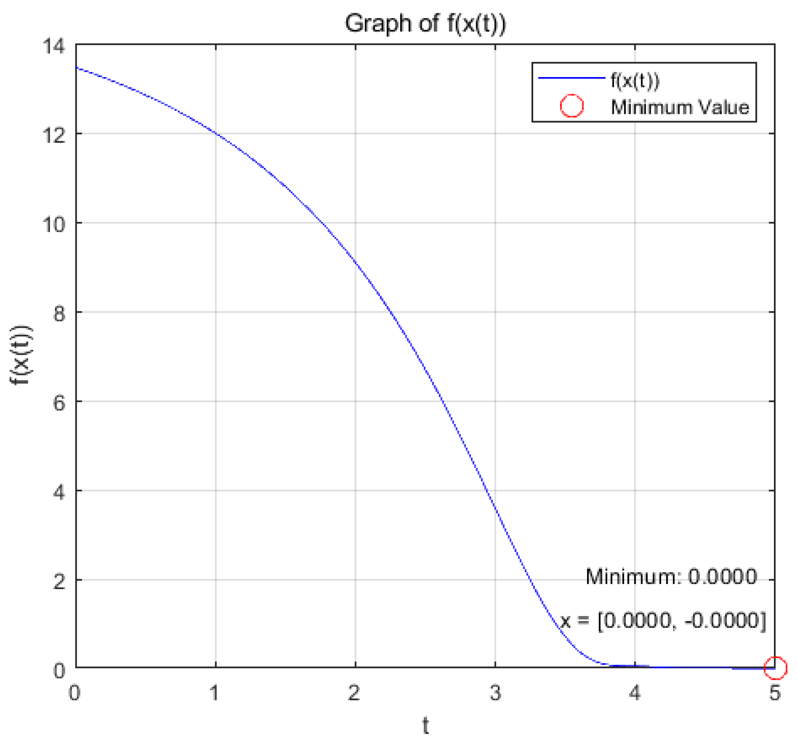
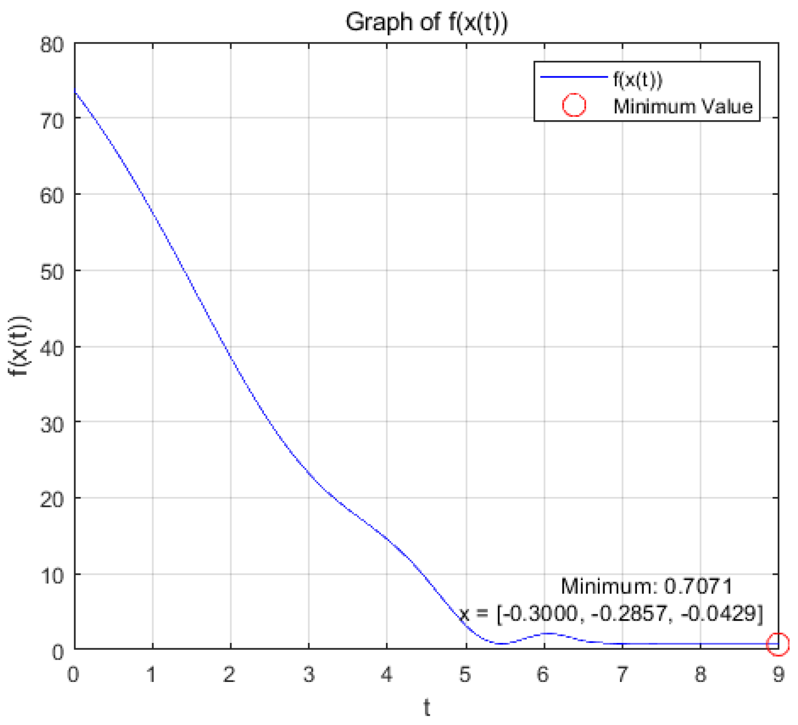
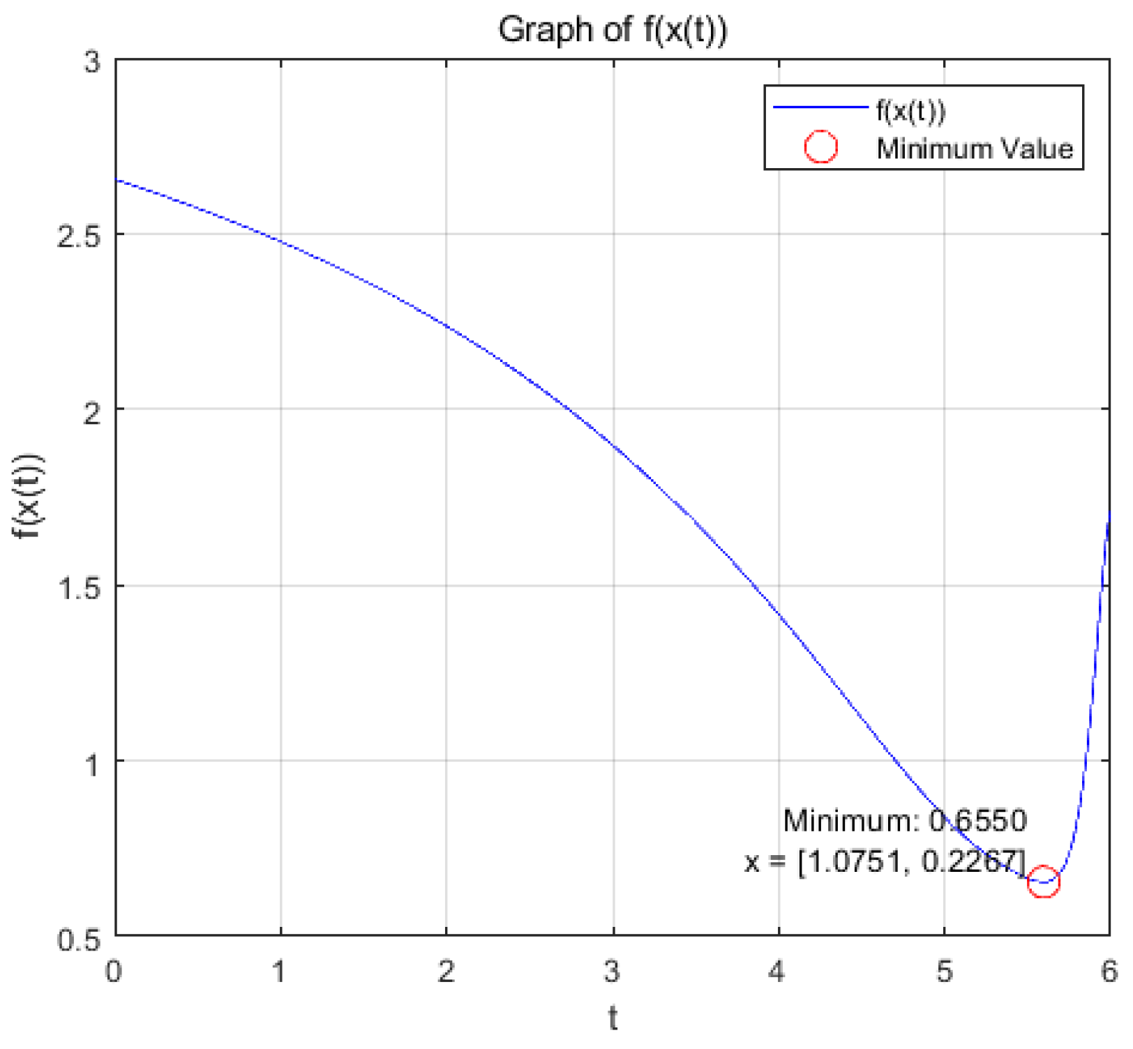
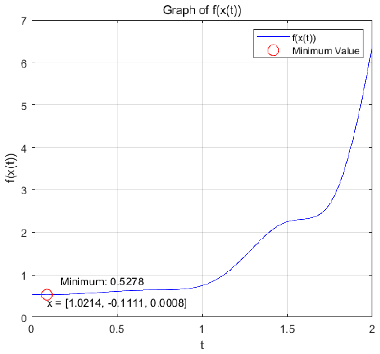
Case 1: when =0.5, a=2, =1, T=6, A=, we choose and , then we consider the minimum of the strongly convex function .
(a): Figure 1 and Figure 2 show the variation of variables x and with respect to t when the system (9) is applied to solve the problem, respectively.
Figure 1.
change with respect to t.
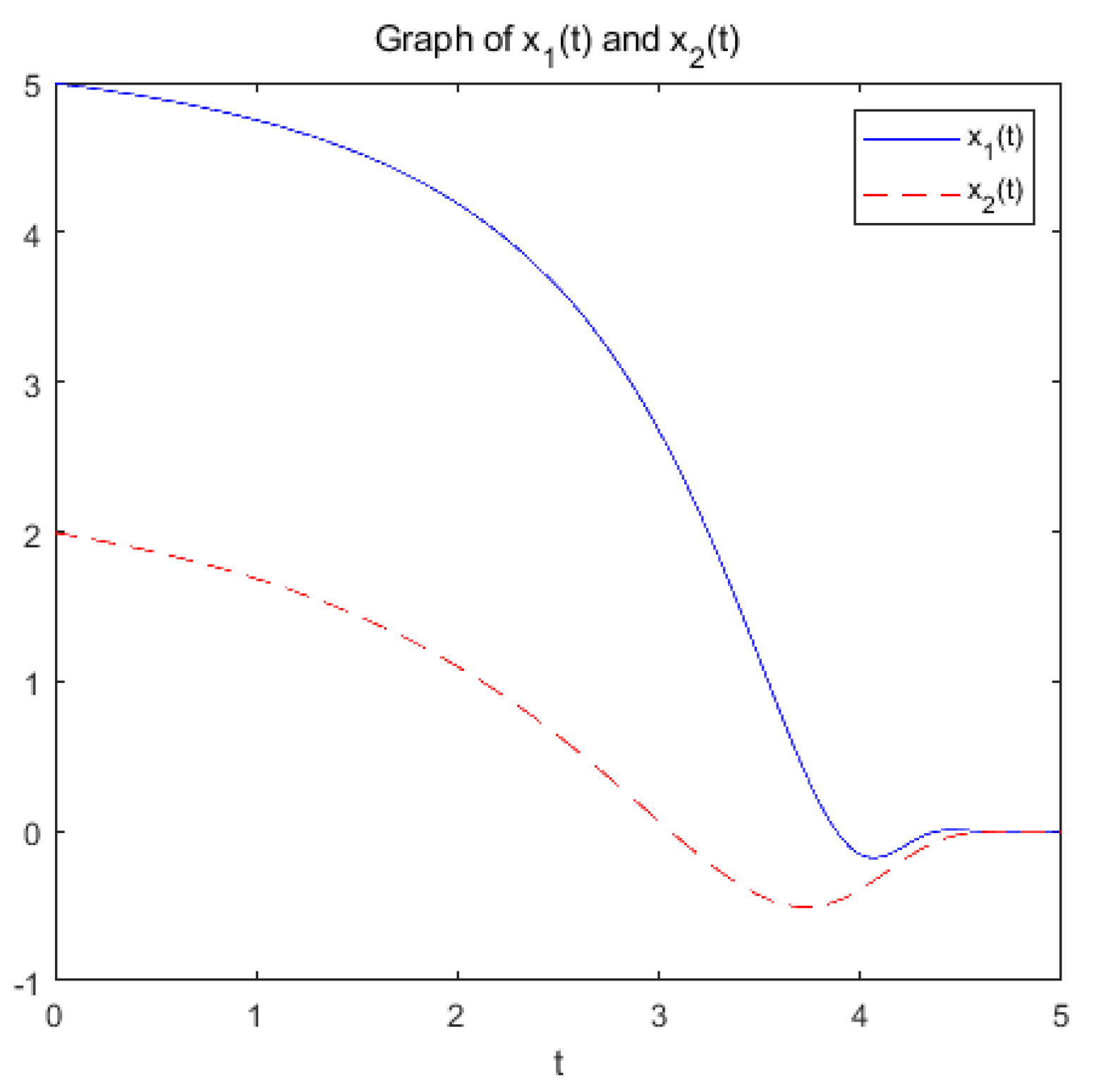
Figure 2.
change with respect to t.
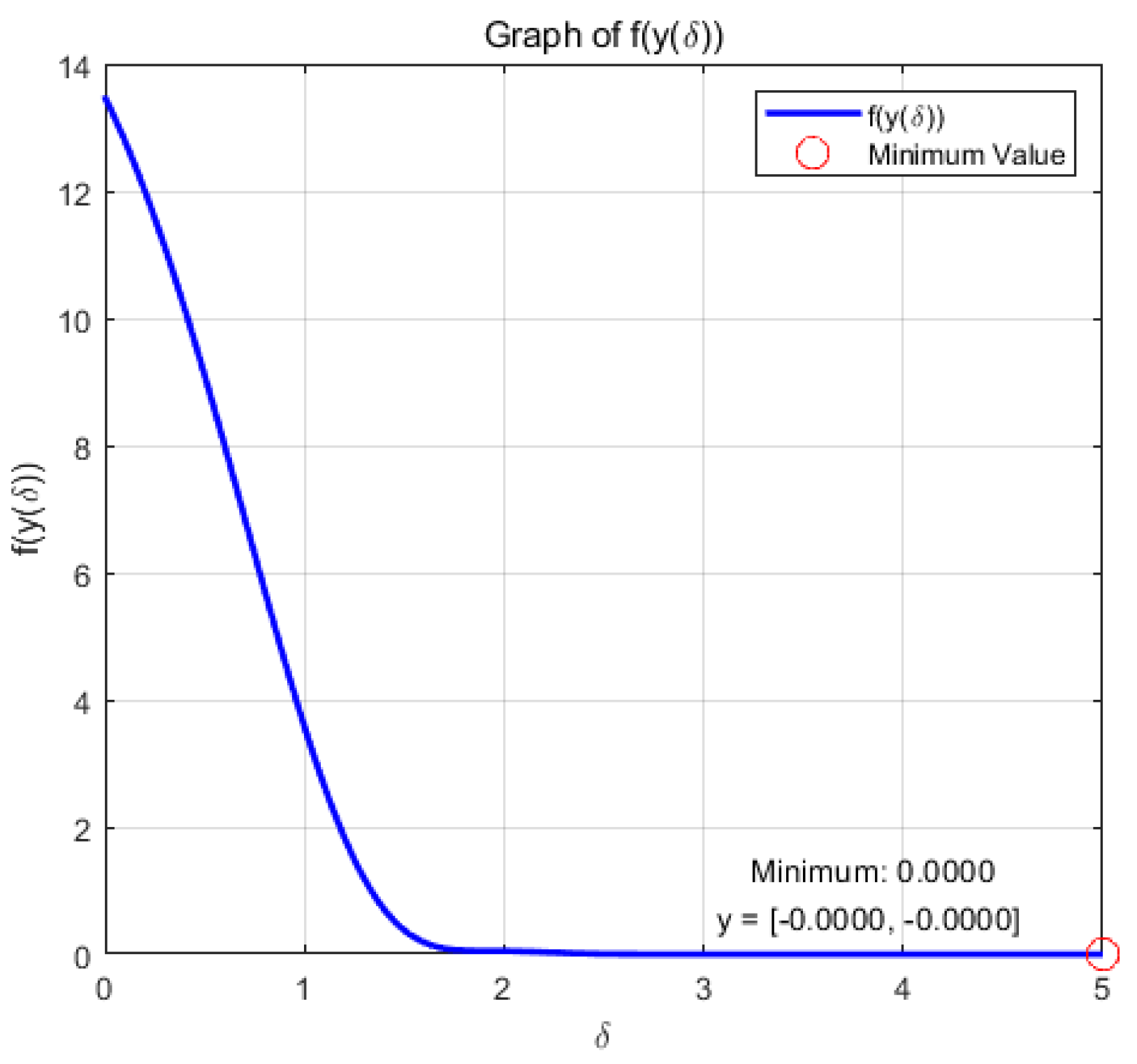
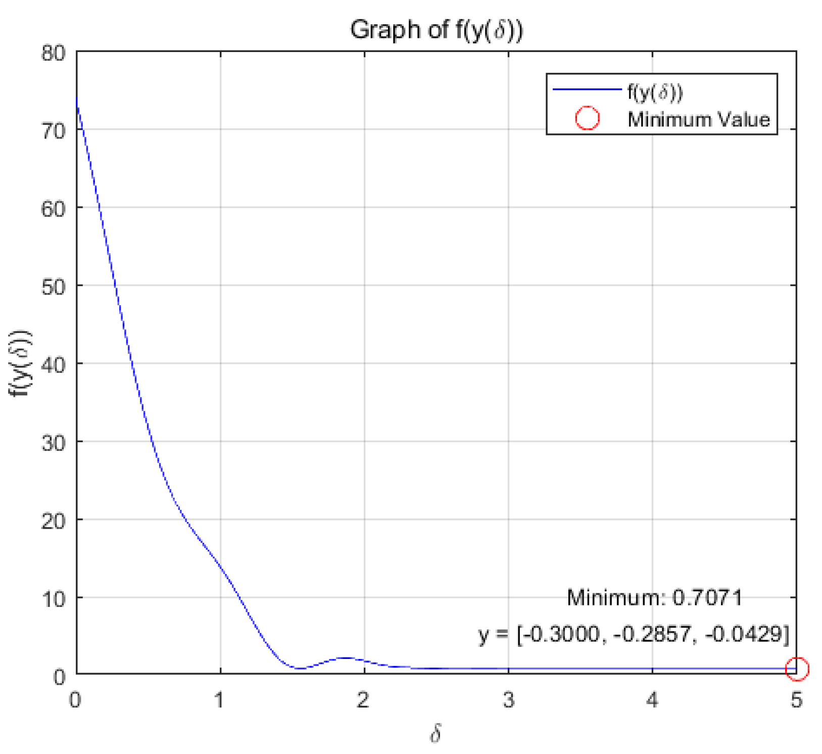
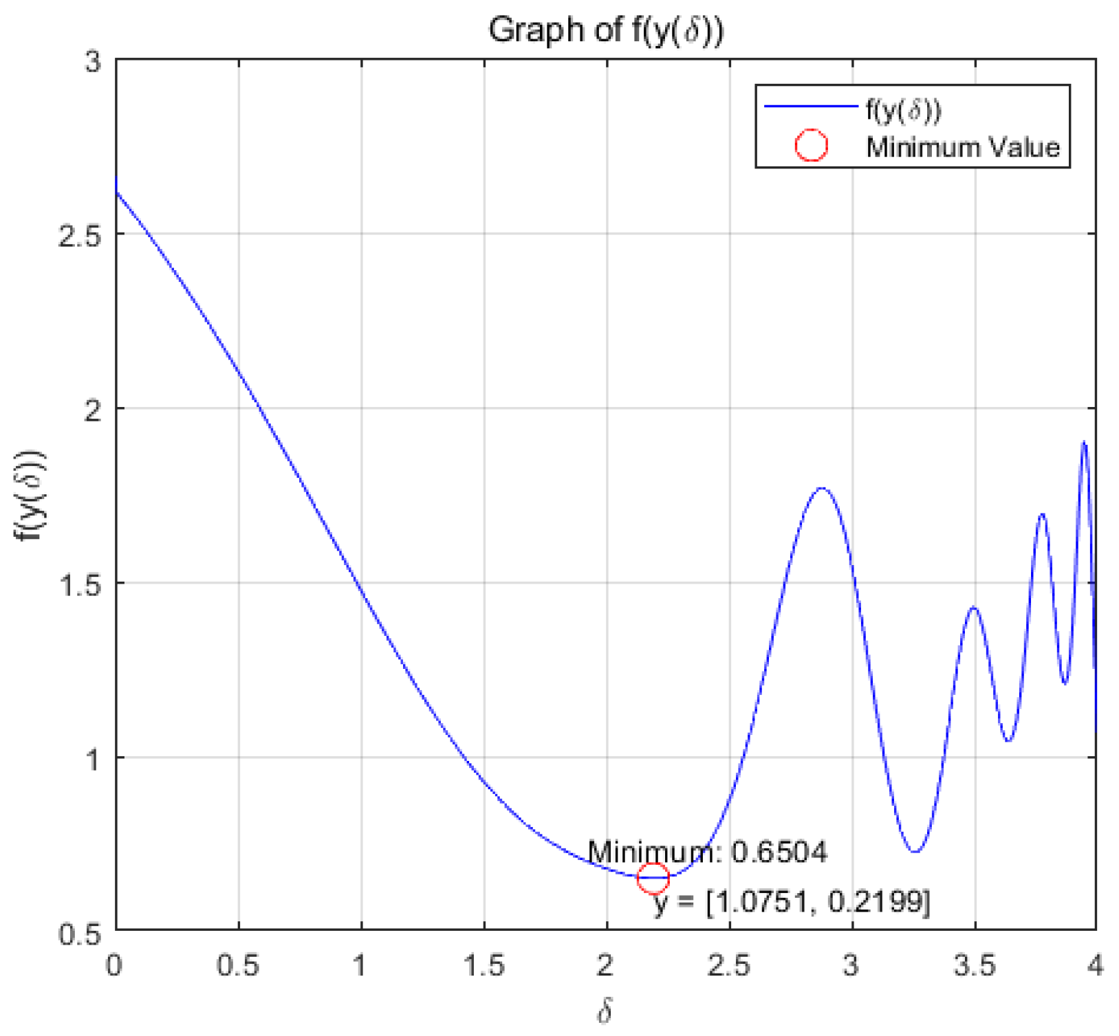
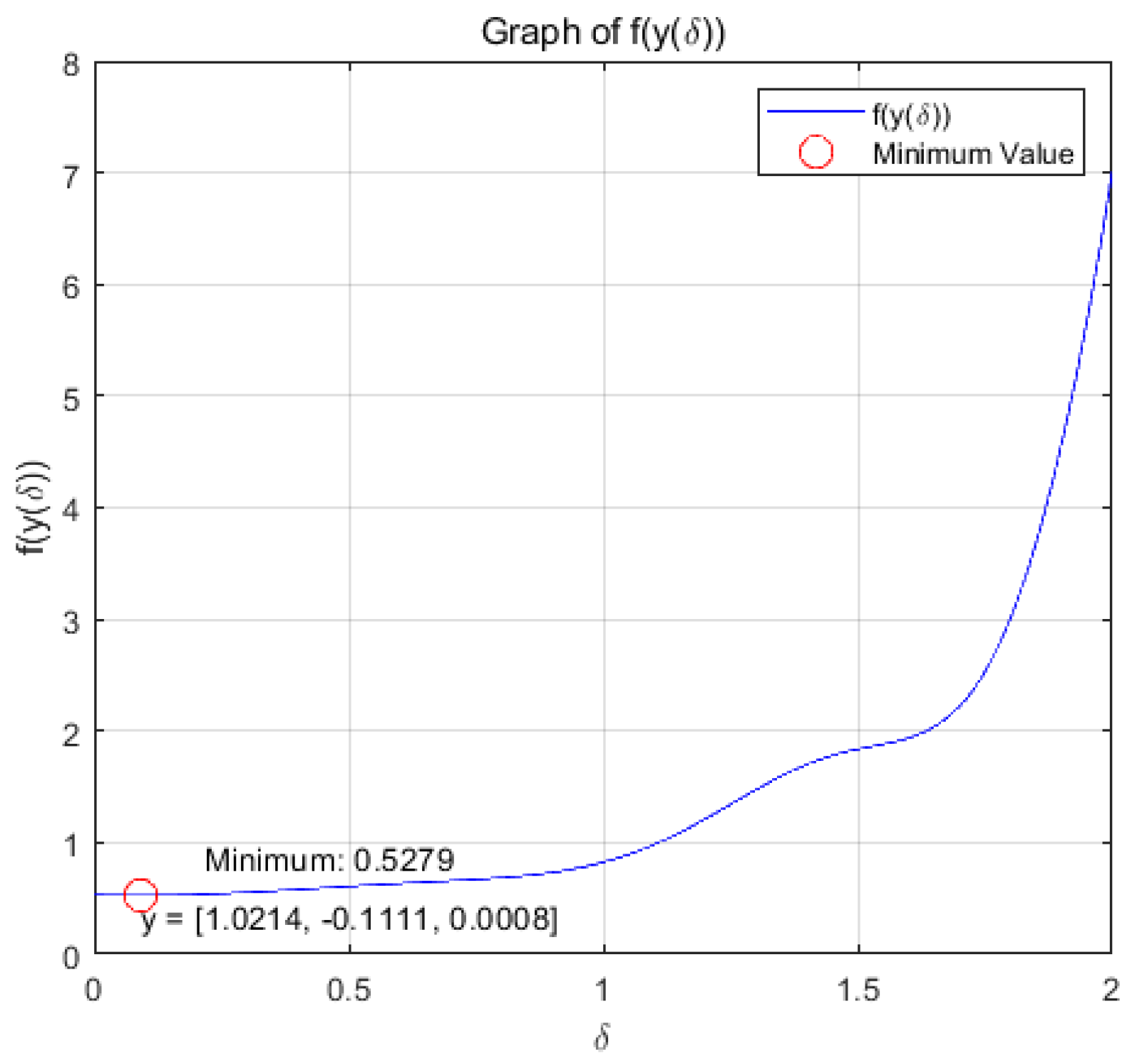
(b): Figure 3 and Figure 4 show the variation of variables y and f(y()) with respect to when the system (14) is applied to solve the problem, respectively.
Figure 3.
change with respect to .
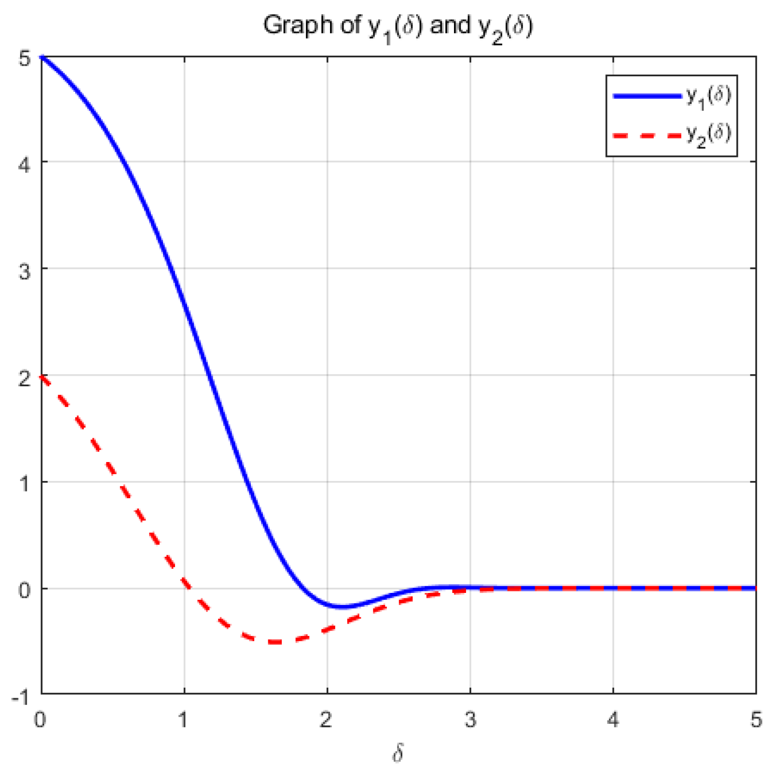
Figure 4.
change with respect to .
Remark 5.
the optimization problem reaches the optimal solution within a prescribed time T=6 under the action of system (9), and the optimization problem of its equivalence converges asymptotically to the same optimal solution under the action of system (14).
Case 2: when =1, a=3, T=9.5, A= c= d=1, b=1/2, we choose and , then we consider the minimum of the strongly convex function .
(a): Figure 5 and Figure 6 show the variation of variables x and with respect to t when the system (9) is applied to solve the problem, respectively.
Figure 5.
change with respect to t.
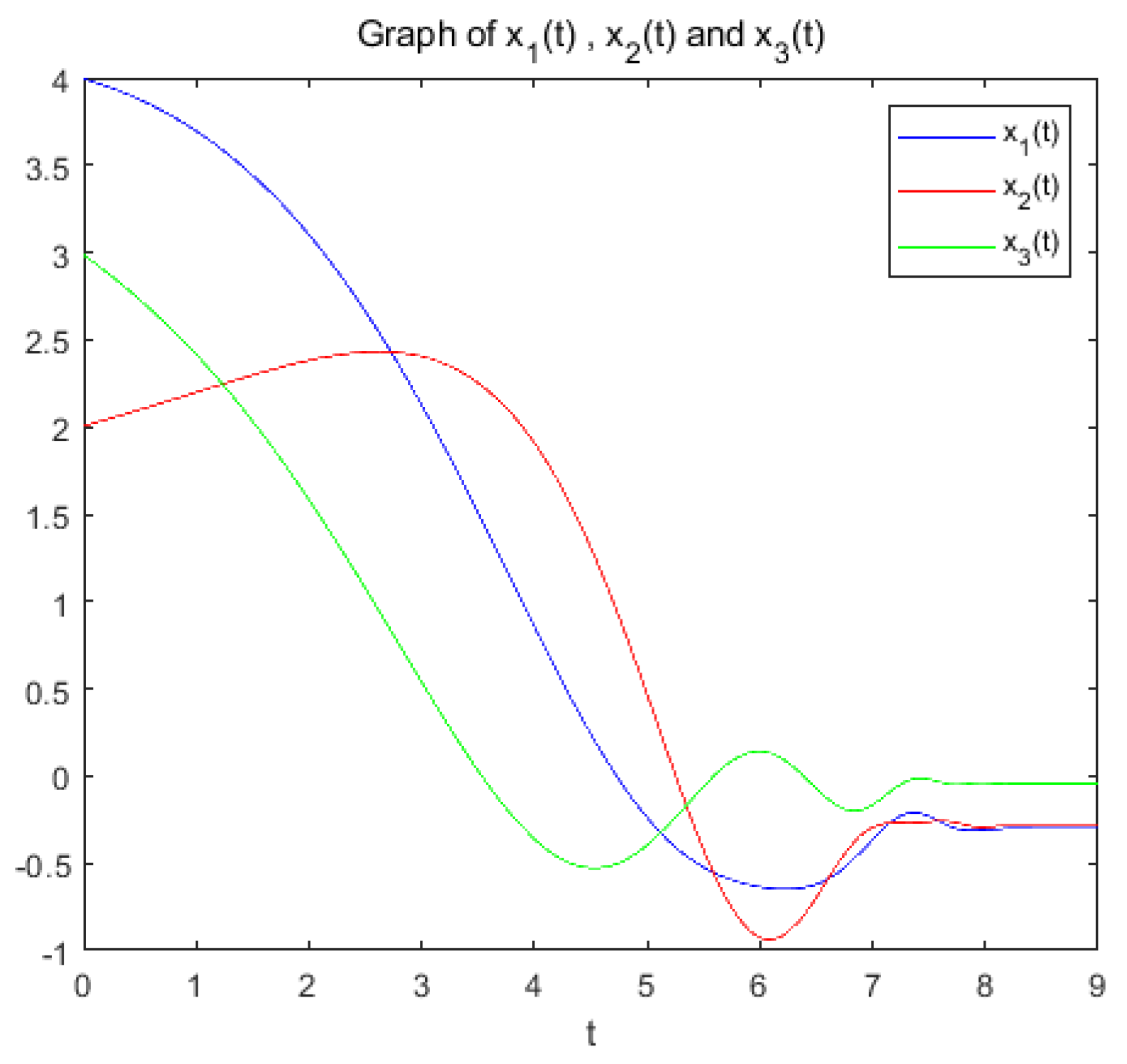
Figure 6.
change with respect to t.
(b): Figure 7 and Figure 8 show the variation of variables y and with respect to when the system (14) is applied to solve the problem, respectively.
Figure 7.
change with respect to .
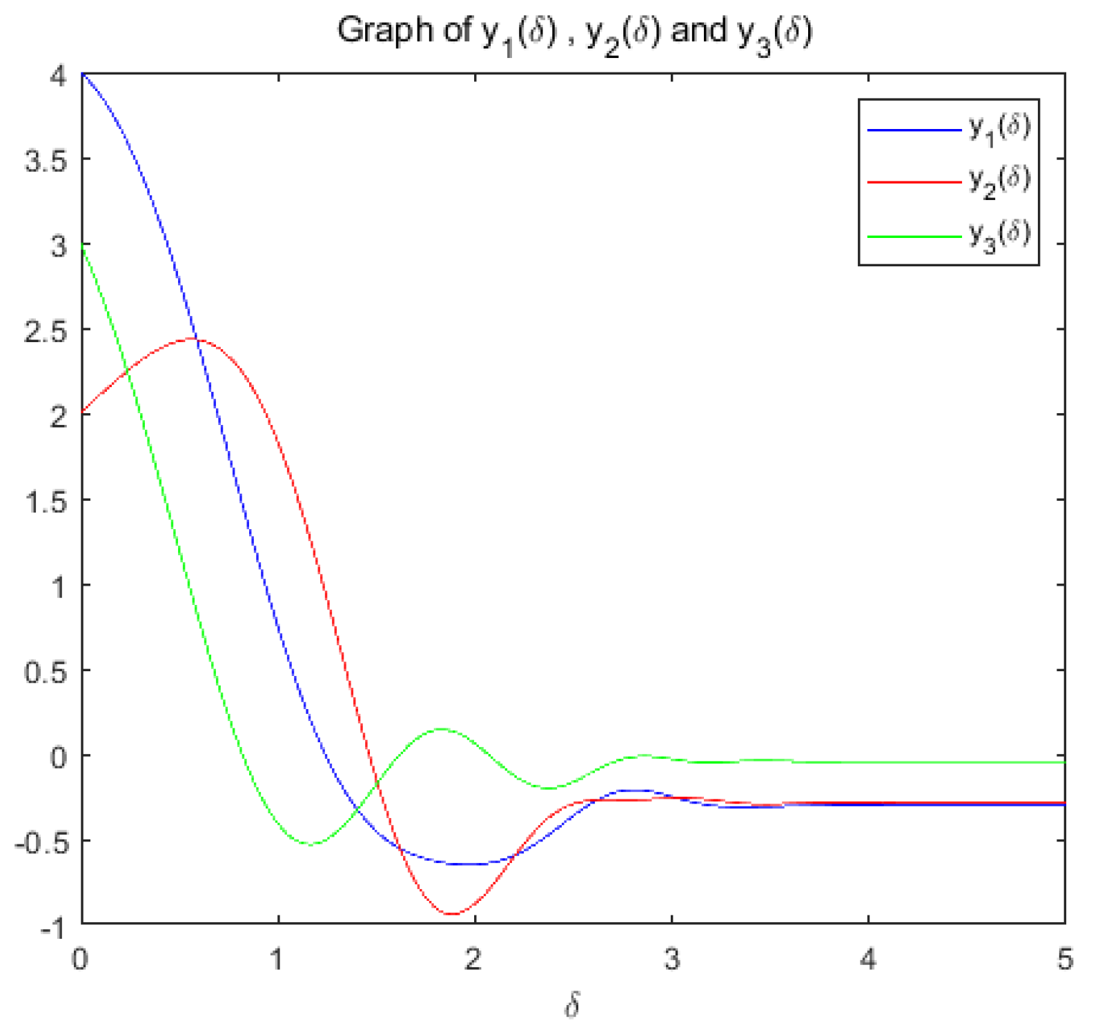
Figure 8.
change with respect to .
Remark 6.
the optimization problem reaches the optimal solution within a prescribed time T=9.5 under the action of system (9), and the optimization problem of its equivalence converges asymptotically to the same optimal solution under the action of system (14).
Case 3: when =1, a=0.5, T=6.5, k=0.9, A=, b=, we choose and , then we consider the minimum of the strongly convex function .
(a): Figure 9 and Figure 10 show the variation of variables x and with respect to t when the system (17) is applied to solve the problem, respectively.
Figure 9.
change with respect to t.
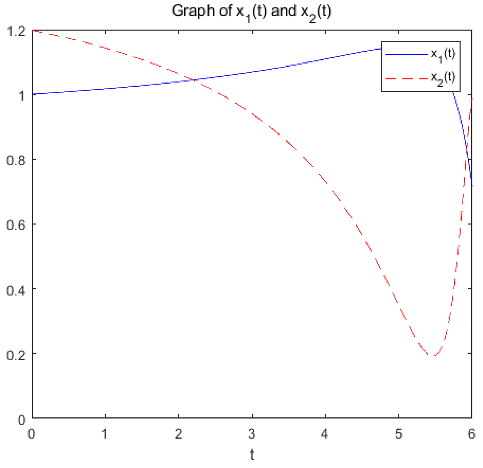
Figure 10.
change with respect to t.
(b): Figure 11 and Figure 12 show the variation of variables y and with respect to when the system (20) is applied to solve the problem, respectively.
Figure 11.
change with respect to .
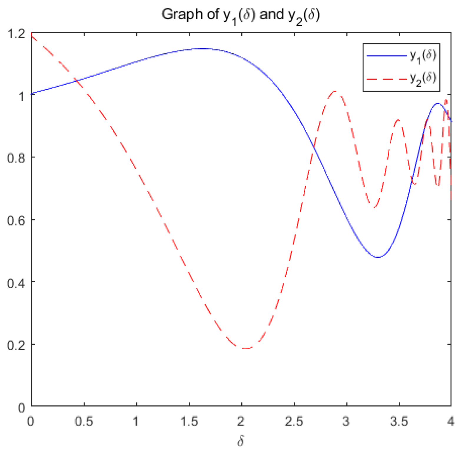
Figure 12.
change with respect to .
Remark 7.
Within the allowable range of error, the optimization problem reaches the optimal solution within a prescribed time T=6.5 under the action of system (17), and the optimization problem of its equivalence converges asymptotically to the same optimal solution under the action of system (20).
Case 4: when =0.35, a=0.8, T=8, A=, b= we choose and , then we consider the minimum of the strongly convex function .
(a): Figure 13 and Figure 14 show the variation of variables x and with respect to t when the system (17) is applied to solve the problem, respectively.
Figure 13.
change with respect to t.
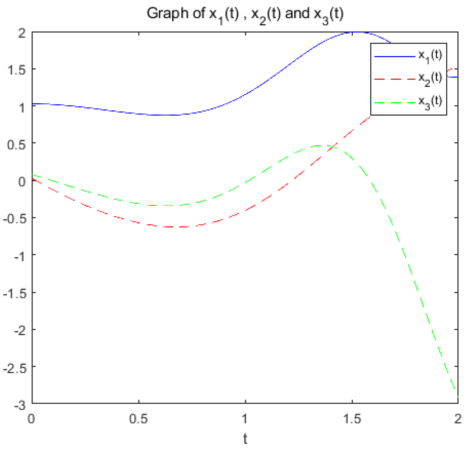
Figure 14.
change with respect to t.
(b): Figure 15 and Figure 16 show the variation of variables y and with respect to when the system (20) is applied to solve the problem, respectively.
Figure 15.
change with respect to .
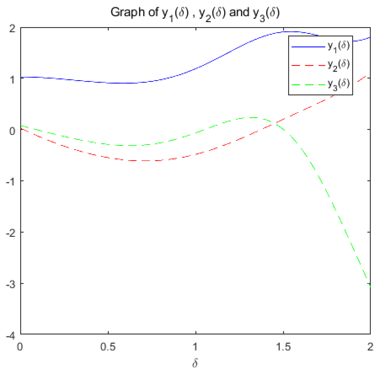
Figure 16.
change with respect to .
Remark 8.
the optimization problem reaches the optimal solution within a prescribed time T=8 under the action of system (17), and the optimization problem of its equivalence converges asymptotically to the same optimal solution under the action of system (20).
7. Conclusions and Future Work
For the unconstrained optimization problem of strongly convex objective function and the optimization problem with equation constraints, we develop a novel prescribed-time convergence acceleration algorithm with time rescaling. Our basic idea is to construct different second-order systems under certain conditions, so that the two types of optimization problems converge to the optimum solution within a prescribed-time T. This is more flexible than the traditional exponential asymptotic time convergence and improves the convergence rate of the algorithm to a large extent. According to this idea, our next work can be focus on
(1) Modify the optimization algorithm with sub-linear convergence rate so that it can also converge to the optimum solution of the optimization problem within a prescribed-time T .
(2) Considering the problem that the strongly convex objective function has a prescribed time T convergence under the constraints of general convex ensembles or inequalities.
(3) In addition to the Euler method, it is possible to discretize a system that converges within a prescribed time T by methods such as Lunger-Kutta.
(4) Consider the problem of acceleration of algorithms that converge in prescribed time T in a distributed manner.
Funding
This research was supported by the National Natural Science Foundation of China (62163035), the Technology Development Guided by the Central Government (ZYYD2022A05), Tianshan Talent Training Program (2022TSYCLJ0004), Ministry of Science and Technology Base and Talent Special Project-Third Xinjiang Scientific Expedition Project (2021xjkk1404).
References
- Polyak, B. Some methods of speeding up the convergence of iteration methods. USSR Computational Mathematics and Mathematical Physics 1964, 4, 1–17. [Google Scholar] [CrossRef]
- Nesterov, Y.E. A method of solving a convex programming problem with convergence rate O(1/k2). Dokl.akad.nauk Sssr 1983, 269. [Google Scholar]
- Nesterov, Y.E. One class of methods of unconditional minimization of a convex function, having a high rate of convergence. USSR Computational Mathematics and Mathematical Physics 1985, 24, 80–82. [Google Scholar] [CrossRef]
- Nesterov, Y.E. An approach to the construction of optimal methods for minimization of smooth convex function. èkonom. i Mat. Metody 1988, 24, 509–517. [Google Scholar]
- Pierro, A.; Lopes, J. Accelerating iterative algorithms for symmetric linear complementarity problems. International Journal of Computer Mathematics 1994, 50, 35–44. [Google Scholar] [CrossRef]
- Arihiro, K.; Satoshi, F.; Tadashi Ae Members. Acceleration by prediction for error back-propagation algorithm of neural network. Systems and Computers in Japan 1994, 25, 78–87. [Google Scholar]
- Beck, A.; Teboulle, M. A fast iterative shrinkage-thresholding algorithm for linear inverse problems. SIAM J. Imaging Sci 2009, 2, 183–202. [Google Scholar] [CrossRef]
- Nesterov, Y.E. Gradient methods for minimizing composite objective function. Technical Report Discussion Paper 2007/76,CORE.
- O’Donoghue, B.; Cand, E. Adaptive restart for accelerated gradient schemes. Found Comput Math 2015, 15, 715–732. [Google Scholar] [CrossRef]
- Nguyen, N.C.; Fernandez, P.; Freund, R.M.; Peraire, J. Accelerated residual methods for the iterative solution of systems of equations. SIAM Journal on Scientific Computing 2018, 40, A3157–A3179. [Google Scholar] [CrossRef]
- Song, Y.; Wang, Y.; Holloway, J.; Krstic, M. Time-varying feedback for regulation of normal-form nonlinear systems in prescribed finite time. Automatica 2017, 83, 243–251. [Google Scholar] [CrossRef]
- Li, H.; Zhang, M.; Yin, Z.; Zhao, Q.; Xi, J.; Zheng, Y. Prescribed-time distributed optimization problem with constraints. ISA Transactions 2024, 148, 255–263. [Google Scholar] [CrossRef] [PubMed]
- Liu, L.; Liu, P.; Teng, Z.; Zhang, L.; Fang, Y. Predefined-time position tracking optimization control with prescribed performance of the induction motor based on observers. ISA Transactions 2024, 147, 187–201. [Google Scholar] [CrossRef] [PubMed]
- Zhang, Y.; Chadli, M.; Xiang, Z. Prescribed-Time Adaptive Fuzzy Optimal Control for Nonlinear Systems. IEEE Transactions on Fuzzy Systems 2024, 32, 2403–2412. [Google Scholar] [CrossRef]
- Attouch, H.; Chbani, Z.; Riahi, H. Fast proximal methods via time scaling of damped inertial dynamics. SIAM J. Optim. 2019, 29, 2227–2256. [Google Scholar] [CrossRef]
- Attouch, H.; Chbani, Z.; Riahi, H. Fast convex optimization via time scaling of damped inertial gradient dynamics. Pure Appl. Funct. Anal. 2021, 6, 1081–1117. [Google Scholar]
- Attouch, H.; Chbani, Z.; Fadili, J.; Riahi, H. First-order optimization algorithms via inertial systems with Hessian driven damping. Math. Program. 2022, 193, 113–155. [Google Scholar] [CrossRef]
- Attouch, H.; Chbani, Z.; Fadili, J.; Riahi, H. Fast convergence of dynamical ADMM via time scaling of damped inertial dynamics. J. Optim. Theory Appl. 2022, 193, 704–736. [Google Scholar] [CrossRef]
- He, X.; Hu, R.; Fang, Y.P. Inertial primal-dual dynamics with damping and scaling for linearly constrained convex optimization problems. Applicable Anal. 2022. [Google Scholar] [CrossRef]
- Balhag, A.; Chbani, Z.; Attouch, H. Fast convex optimization via inertial dynamics combining viscous and Hessian-driven damping with time rescaling. Evolution Equations and Control Theory 2022, 11, 487–514. [Google Scholar]
- Hulett, D.A.; Nguyen, D-K. Time Rescaling of a Primal-Dual Dynamical System with Asymptotically Vanishing Damping. Applied Mathematics Optimization 88 2023, 27. [Google Scholar] [CrossRef]
- Luo, H. A primal-dual flow for affine constrained convex optimization. ESAIM: Control,Optimisation Calculus of Variations 2022, 28, 1–34. [Google Scholar] [CrossRef]
- Luo, H.; Chen, L. From differential equation solvers to accelerated first-order methods for convex optimization. Mathematical Programming 2021, 195, 1–47. [Google Scholar] [CrossRef]
- Chen, L.; Luo, H. A unified convergence analysis of first order convex optimization methods via strong lyapunov functions. arXiv:2108.00132.
- Luo, H. Accelerated primal-dual methods for linearly constrained convex optimization problems. arXiv:2109.12604v2.
- Tran, D.; Yucelen, T. Finite-time control of perturbed dynamical systems based on a generalized time transformation approach. Systems Control Letters 2020, 136, 104605. [Google Scholar] [CrossRef]
Disclaimer/Publisher’s Note: The statements, opinions and data contained in all publications are solely those of the individual author(s) and contributor(s) and not of MDPI and/or the editor(s). MDPI and/or the editor(s) disclaim responsibility for any injury to people or property resulting from any ideas, methods, instructions or products referred to in the content. |
© 2024 by the authors. Licensee MDPI, Basel, Switzerland. This article is an open access article distributed under the terms and conditions of the Creative Commons Attribution (CC BY) license (http://creativecommons.org/licenses/by/4.0/).
Copyright: This open access article is published under a Creative Commons CC BY 4.0 license, which permit the free download, distribution, and reuse, provided that the author and preprint are cited in any reuse.


