
Submitted:
06 September 2025
Posted:
09 September 2025
You are already at the latest version
Abstract
The integration of photovoltaic (PV) systems into power grids has surged due to the global shift towards renewable energy, but this rapid adoption presents challenges like voltage regulation and inverter degradation. High PV penetration can lead to overvoltage conditions and transient voltage fluctuations, which stress inverters and accelerate their degradation. To address these issues, advanced modeling techniques, particularly Bayesian modeling, are employed to predict and mitigate inverter failures by incorporating prior knowledge and real-world data. This approach enables probabilistic predictions of failure, improving maintenance scheduling and inverter design. By leveraging datasets from inverter operations with induction motors, this study aims to enhance the reliability of PV systems and optimize voltage regulation strategies for sustainable renewable energy growth.
Keywords:
bayesian degradation modeling
; PV inverter failure
; induction motor drives
; voltage instability
; predictive maintenance
1. Introduction
Inverters are fundamental components of photovoltaic systems, primarily responsible for converting the direct current (DC) electricity generated by solar panels into alternating current (AC) suitable for grid use [1]. This conversion is essential, as most electrical appliances and the power grid operate on AC electricity. By enabling the integration of solar energy into the electrical grid, inverters facilitate the utilization of renewable energy sources, contributing to a more sustainable energy landscape.
In addition to their primary function, PV inverters provide ancillary services such as reactive power compensation and voltage stabilization [2]. These services are crucial for maintaining grid stability, especially in areas with high penetration of solar energy. By managing voltage levels and supporting reactive power needs, inverters help ensure that the electricity supplied to the grid remains reliable and within acceptable limits, thereby enhancing the overall performance and resilience of the power system.
By comparing the working principles and degradation mechanisms of inverters in these applications, this article provides insights into their implications for power systems. Understanding these differences is crucial for optimizing inverter design and ensuring the reliable operation of both renewable energy systems and industrial motor-driven processes.
This article compares the challenges faced by inverters in photovoltaic systems and induction motor systems. While inverters are crucial in both contexts, their operational demands, degradation mechanisms, and impacts on the power system differ significantly.
1.1. Overall Inverter Performance
The performance of inverters is crucial in both photovoltaic systems and induction motor applications. This section discusses the operational characteristics, efficiency, and degradation mechanisms of inverters in these contexts.
Figure 1 presents a comprehensive overview of the inverter configurations utilized in photovoltaic and induction motor applications.
In PV systems, the inverter is primarily responsible for converting direct current (DC) generated by solar panels into alternating current (AC) for use in electrical loads or grid connection [3]. The operation is relatively steady-state, as the inverter adapts to varying environmental conditions such as solar irradiance and temperature.
In contrast, the inverter used in induction motor applications incorporates an additional Pulse-Width Modulation (PWM) controller [4]. This controller is vital for dynamically adjusting the output frequency and voltage, enabling precise control over the motor’s speed and torque. The PWM technique allows for efficient operation under varying load conditions, making it indispensable for applications requiring high performance and responsiveness.
Previous research on inverter degradation has primarily relied on deterministic or heuristic analysis methods, typically focusing on single application areas such as photovoltaic (PV) systems or motor drives. In contrast to these approaches, this work introduces a unified statistical degradation modeling framework that leverages information criteria (AIC/BIC) and real-world operational inverter data.
The novelty of our approach lies in conducting a comparative degradation analysis across both PV and motor drive applications, enabling the identification of shared degradation mechanisms and their impact on control strategies. This perspective provides new, practical insights that have not been widely discussed in the existing literature.
1.2. Degradation Mechanisms in Inverters
Inverters, regardless of their application, are subject to degradation over time due to various factors. Figure 2 provides an overview of the primary degradation mechanisms affecting inverter performance.
While PV inverters are optimized for steady-state operation under varying environmental conditions, motor inverters are designed for dynamic performance and precise control. Both types of inverters require regular maintenance and monitoring to ensure long-term reliability. Advanced diagnostic techniques, such as machine learning models, have been proposed to predict inverter efficiency degradation and optimize maintenance schedules.
1.2.1. Role of Inverters in Induction Motors
Inverters are essential components in induction motor systems, primarily responsible for controlling motor speed and torque by varying the output voltage and frequency [5]. This capability allows for precise adjustments in motor performance, enabling efficient operation across a range of industrial applications, such as pumps, conveyors, and HVAC systems. By facilitating smooth acceleration and deceleration, inverters enhance energy efficiency and reduce mechanical stress on motor components, ultimately leading to improved reliability and longevity of the motor systems [6]. Their ability to adapt to varying load conditions further underscores their importance in modern industrial automation, where precision and efficiency are paramount.
1.2.2. Operational Factors Affecting Performance
Table 1 outlines the various degradation mechanisms specific to induction motor inverters.
Table 1 details the causes of degradation, such as thermal overload and mechanical stress, along with their negative effects on motor performance and lifespan. These insights are essential for developing effective maintenance strategies and enhancing the operational reliability of induction motors.
Voltage regulation is a critical challenge in microgrids, particularly in systems with high penetration of photovoltaic (PV) energy. During peak solar generation, overvoltage conditions can occur due to the excess active power injected into the grid, which exceeds the local demand. This imbalance can lead to voltage instability at various nodes within the microgrid, as observed in voltage rate data from transformers and nodes.
1.3. Related Works
Recent literature highlights the importance of identifying and quantifying technical risks associated with photovoltaic power systems, including inverter degradation. Ref. [11] provide a comprehensive framework for analyzing and mitigating such risks, emphasizing the need for systematic approaches to ensure long-term system reliability.
Ref. [12] investigate how environmental factors—specifically light, heat, and humidity—accelerate the degradation of PV components. While their focus is on the overall PV system, these stressors are also known to impact inverter performance and lifespan, suggesting that environmental testing is crucial for predicting inverter degradation.
The integration of predictive maintenance strategies is gaining traction as a means to address inverter degradation. Ref. [13] utilize SCADA data and machine learning to detect anomalies in PV systems, enabling early identification of inverter faults. Similarly, ref. [14] propose trend-based analytics for predictive maintenance and fault detection, further supporting the proactive management of inverter health.
Advanced control schemes play a significant role in mitigating the effects of inverter degradation. Ref. [15] present a coordinated control approach for voltage regulation and power management in multibus DC microgrids, which can help maintain system stability even as inverter performance declines. Ref. [16] extend this by introducing hierarchical control with voltage balancing and energy management, offering robust solutions to counteract the negative impacts of inverter aging in bipolar DC microgrids.
Collectively, these studies underscore the multifaceted nature of inverter degradation in distributed power systems. They highlight the need for comprehensive risk assessment, environmental testing, predictive maintenance, and advanced control strategies to ensure the reliability and longevity of inverters within PV and microgrid applications.
Central Research Question
Our central question is: which parsimonious distributional models best characterize degradation-related variability in inverter voltage, current, and active power under operational stress, and how do these patterns compare between PV and induction-motor contexts? We address this by fitting linear and distributional models (Normal, Log-normal, Gamma, Poisson) to three-phase measurements and selecting models via AIC/BIC.
The rest of the paper is organised as follows. Section 2 describes the data, operating context, and preprocessing pipeline. Section 2 also details the modelling framework and inference procedures, including model selection via AIC/BIC. Section 3 reports empirical results for voltage, current, and active power (Figure 3, Figure 4 and Figure 5). Section 4 discusses implications, and Section 5 concludes.
2. Methods and Materials
This section outlines the methodology used to assess inverter degradation under operational stress. A combination of statistical modeling and comparative analysis was used to evaluate the reliability of inverter systems in PV and induction motor applications.
Analysis pipeline. We follow a stepwise pipeline: (1) data acquisition; (2) preprocessing (outlier removal, normalization, per-phase segmentation); (3) distributional model fitting (Normal, Log-normal, Gamma, Poisson) alongside linear trend baselines; (4) model selection using AIC and BIC; (5) diagnostics (residual behavior, tails, support compatibility); (6) synthesis across variables and phases to inform monitoring recommendations.
2.1. Data Source and Preprocessing
This study utilized operational data from inverter-fed induction motor systems. The datasets included time-series measurements of voltage, current, power, and active power across three phases. This data was collected via IoT devices from June 25th, 2019 to April 14th, 2020, with measurements sampled every 15 minutes (equivalent to a frequency of approximately 0.0011 Hz), resulting in a total duration of about 294 days or roughly 423,360 samples. The documentation of the analyzed study does not specify the models or manufacturers of the inverters used, nor does it clarify whether the inverters are industrial, laboratory, or prototype devices.
The data was preprocessed by removing outliers and normalizing each time series to facilitate statistical modeling. Each signal was segmented by operational phase (Phase A, B, C), and descriptive statistics (minimum, maximum, mean) were computed as a baseline for model evaluation.
Scope and Limitations
Documentation for the analyzed datasets does not specify inverter models/manufacturers nor deployment class (industrial/laboratory/prototype). We therefore delimit claims to statistical behavior of the measured variables under observed operating conditions rather than to any specific make or standard.
2.2. Statistical Modelling Approach
To assess inverter degradation patterns, several statistical models were applied to the voltage, current, power, and active power signals. The evaluated models include:
- Linear regression
- Normal distribution
- Log-normal distribution
- Gamma distribution
- Poisson distribution
Linear regression models the relationship between two variables (e.g., time and voltage, or current and power) assuming a straight-line relationship [17]. It provides a simple and interpretable model for trends in data, such as how voltage or current changes over time or with other variables [18]. Linear regression assumes normally distributed residuals, which ties it to the normal distribution.
The normal distribution is used to model symmetric, bell-shaped data, such as voltage or current fluctuations around a mean value [19] It describes the probability of observing certain values of voltage, current, or power, assuming the data is symmetric and centered around a mean [20]. The normal distribution is the foundation for many statistical models, including linear regression. It assumes that the data is not skewed.
The log-normal distribution models data where the logarithm of the variable is normally distributed. This is useful for skewed data, such as power or active power, which cannot take negative values [21]. It captures the behavior of variables that grow multiplicatively or have a long right tail, such as power consumption or current in certain systems [22]. The log-normal distribution is related to the normal distribution but is used for skewed data. It is often applied when a normal distribution fails to fit the data due to skewness.
The Gamma distribution models continuous, positive data with skewness, such as power or current. It is often used when the variance increases with the mean [23]. It captures the variability in power or current data that cannot be explained by simpler models like the normal distribution. For example, it can model power consumption over time or current fluctuations in a circuit [24]. The Gamma distribution is related to the log-normal distribution in that both handle skewed data. However, the Gamma distribution is more flexible for modeling variance that increases with the mean.
The Poisson distribution models count data or discrete events occurring over time or space. It is often used for voltage or current spikes or discrete power events [25]. It describes the probability of observing a certain number of events (e.g., voltage spikes) in a fixed interval. It is particularly useful for modeling rare events [26]. The Poisson distribution is part of the exponential family, like the Gamma distribution. It is also related to the normal distribution for large counts (via the Central Limit Theorem).
The Gamma distribution is suitable for modeling continuous, positive data such as power and current, especially when the data is skewed. In contrast, the Poisson distribution is used for discrete events, such as voltage spikes or current surges, describing the probability of observing a certain number of events in a fixed interval.
2.3. Information Criteria
Inverter degradation involves complex interactions between operational stressors and component wear. By applying AIC and BIC to models built on real-world datasets (e.g., those incorporating induction motor operations), researchers can identify the best-fitting models to predict degradation patterns [27]. AIC might favor models that capture subtle degradation trends, while BIC might prioritize simpler models that generalize better across different conditions.
AIC evaluates models by estimating the relative amount of information lost when using a model to represent the data. It penalizes models with more parameters to discourage overfitting, making it particularly useful for capturing the nuanced behavior of inverters under varying operational conditions, such as voltage fluctuations and load variability [28]. For example, in modeling inverter degradation, AIC can help select a model that accurately predicts failure rates without introducing unnecessary complexity.
BIC is similar to AIC but applies a stricter penalty for model complexity, especially as the dataset size increases [29]. This makes BIC ideal for selecting simpler models that still explain the data well, which is crucial when working with large datasets from inverter operations [30]. By favoring parsimonious models, BIC ensures that the selected model remains interpretable and avoids overfitting, which is critical for long-term reliability analysis.
Building upon prior presentations (e.g., Baranowski, 2025 webinar on statistical degradation modeling), this study further distinguishes itself by applying a structured Bayesian methodology to enable probabilistic inference and uncertainty quantification in the comparative analysis of PV and industrial inverter systems.
Through this approach, we not only identify common and sector-specific degradation mechanisms but also evaluate their implications for control and maintenance strategies. Such a comparative, Bayesian perspective provides a deeper and more technically robust understanding of inverter reliability, filling a notable gap in the recent literature.
Building upon prior presentations, this study formalizes a comparative, distribution-aware selection procedure over real operational data (PV and induction-motor contexts) using AIC/BIC, and ties the selection to Bayesian inference for uncertainty-aware maintenance insights. This positions the contribution beyond tutorial material by delivering a unified, quantitative selection framework applied to multi-phase signals.
2.4. Modelling Tools and Implementation
All statistical models were implemented in Python using the SciPy and Statsmodels libraries. Model fitting and AIC/BIC computations were performed using maximum likelihood estimation. Data visualization was conducted using Matplotlib and Seaborn libraries.
The models were applied separately to each operational phase (A, B, C), and the best-fitting model for each variable was selected based on the lowest AIC and BIC values.
2.5. Modelling Assumptions
For all modeling cases, it was assumed that:
- The operational conditions were stable over each recording window.
- No component replacements or reconfigurations occurred during the measurements.
- Measurement noise was Gaussian and independently distributed.
- Power and current signals were treated as continuous, while voltage spikes were considered for potential Poisson modeling (though ultimately found unsuitable).
3. Results
In this section, we present the degradation behavior of the inverter through three key electrical parameters: voltage, current, and active power. These parameters are critical indicators of inverter health and performance over time. We summarize model viability by reporting per-variable, per-phase AIC/BIC along with representative fits (Figure 3, Figure 4 and Figure 5). Across voltage, current, and active power, Log-normal provides the most consistent fit among continuous distributions, while Poisson is not applicable to quasi-continuous magnitudes.
3.1. Viability of Statistical Models
Each model was fitted to the measured signals from all three phases. Model selection was based on Akaike Information Criterion (AIC) and Bayesian Information Criterion (BIC), which penalize model complexity and quantify the goodness of fit.
Figure 3, Figure 4 and Figure 5 illustrate the degradation trends modeled for each parameter respectively.
Figure 3 shows that, across phases, the Log-normal model yields the lowest AIC/BIC and most faithfully captures the mild right-skew and occasional tail excursions in the voltage measurements. The Gaussian alternative, by enforcing symmetry, systematically underestimates tail risk, while Gamma—despite its positive support—does not outperform Log-normal in these data. Poisson is mis-specified for quasi-continuous magnitudes and is reported only for completeness. Linear regression remains useful as a coarse trend baseline but does not describe distributional shape. These conclusions are consistent with the per-phase comparisons in Table 2.
Current exhibits higher short-term volatility and intermittent bursts than voltage. Correspondingly, the Log-normal model consistently attains the best information criteria, accommodating right-tailed fluctuations observed during load and disturbance episodes. Gaussian fits tend to smooth or under-represent these bursts, and Gamma does not surpass Log-normal on AIC/BIC. As current magnitudes are effectively continuous at the sampling rate, Poisson is not applicable. Linear regression captures mean shifts but misses the bursty character of the process. The ranking in Table 3 supports this assessment.
Active power is the most dynamic of the analyzed signals, reflecting both operating demand and condition. In line with Figure 3 and Figure 4, Log-normal provides the best overall description (lowest AIC/BIC), capturing skew and intermittent surges. Linear regression is informative for slow envelope shifts but not for distributional variability, while Gaussian and Gamma under-capture extremes. Poisson, being a count model, is inapplicable to quasi-continuous values at this resolution. Table 5 corroborates these findings across phases.
Table 2 summarizes the results for voltage in time across all models.
Table 2 compares various models for predicting voltage over time, highlighting their strengths and weaknesses through AIC and BIC metrics. The linear model, while straightforward, has high AIC and BIC values, indicating a poor fit for the data. Similarly, the normal distribution assumes symmetry but struggles with skewed datasets, reflected in its elevated AIC and BIC values.
In contrast, the log-normal distribution performs better with skewed data, showing significantly lower AIC and BIC values. Other models, like the Gamma distribution, are suitable for positive data but do not surpass the log-normal model. The Poisson distribution is not applicable to continuous voltage data, resulting in infinite AIC and BIC values, underscoring the need for careful model selection based on data characteristics.
Table 3 summarizes the results for current in time across all models.
Table 3 provides a comparison of different models for analyzing current data. The linear and normal models exhibit similar performance but are inadequate for capturing skewness in the data, which can lead to suboptimal results in modeling.
In contrast, the log-normal distribution is more effective for skewed current data, as evidenced by its lower AIC and BIC values, indicating a better fit. On the other hand, the Gamma and Poisson models are not suitable for current data, with the Poisson model yielding infinite AIC and BIC values, highlighting its inapplicability to this context.
Table 4 summarizes the results for power in time across all models.
Table 4 compares the performance of models for predicting power over time using AIC and BIC metrics. The linear and normal models perform similarly but show high AIC and BIC values, indicating a poor fit. The log-normal distribution, with significantly lower AIC and BIC values, is better suited for skewed power data.
The Gamma distribution, while appropriate for positive data, does not outperform the log-normal model. The Poisson model, being unsuitable for continuous power data, results in infinite AIC and BIC values, emphasizing its inapplicability.
Table 5 summarizes the results for active power across all models.

Table 5.
AIC/BIC comparison of statistical models for active power across three phases. Poisson is not applicable to quasi-continuous values; log-normal yields the lowest criteria.
Table 5.
AIC/BIC comparison of statistical models for active power across three phases. Poisson is not applicable to quasi-continuous values; log-normal yields the lowest criteria.
| Model | Phase | Min | Max | Average | AIC | BIC |
|---|---|---|---|---|---|---|
| Linear | A | -2976.961 | 3626.644 | 94.839 | 3724558 | 3724589 |
| B | -2583.185 | 3688.165 | 95.983 | 3712701 | 3712732 | |
| C | -2626.442 | 3962.193 | 92.886 | 3726838 | 3726869 | |
| Normal | A | -2976.961 | 3626.644 | 94.839 | 3724558 | 3724589 |
| B | -2583.185 | 3688.165 | 95.983 | 3712701 | 3712732 | |
| C | -2626.442 | 3962.193 | 92.886 | 3726838 | 3726869 | |
| Log-Normal | A | -13.816 | 8.196 | -3.970 | 1739614 | 1739645 |
| B | -13.816 | 8.213 | -4.095 | 1740573 | 1740604 | |
| C | -13.816 | 8.285 | -4.049 | 1740519 | 1740550 | |
| Gamma | A | 0 | 3626.644 | 302.853 | Inf | Inf |
| B | 0 | 3688.165 | 300.030 | Inf | Inf | |
| C | 0 | 3962.193 | 304.167 | Inf | Inf | |
| Poisson | A | 0 | 3626.644 | 302.853 | Inf | Inf |
| B | 0 | 3688.165 | 300.030 | Inf | Inf | |
| C | 0 | 3962.193 | 304.167 | Inf | Inf |
Table 5 presents a comparison of various models for analyzing active power data. The linear and normal models show similar performance but are inadequate for capturing the skewness present in the data, which can lead to inaccurate predictions.
In contrast, the log-normal distribution is more effective for skewed active power data, as indicated by its significantly lower AIC and BIC values. This suggests that it provides a better fit for the data compared to the other models. Meanwhile, the Gamma and Poisson models are not well-suited for active power data, with the Poisson model yielding infinite AIC and BIC values, highlighting its inapplicability in this context.
The figures and tables demonstrate that increased voltage caused by the operation of an induced motor negatively impacts the performance of the connected inverter. This issue arises due to the inverter’s inability to handle the fluctuating voltage levels effectively. A similar situation occurs in photovoltaic systems, where voltage rates vary significantly between periods of power generation during sunlight exposure and times without sunlight. These variations can lead to performance inefficiencies and highlight the importance of designing systems capable of adapting to such dynamic conditions.
3.2. Voltage Regulation Issues in Microgrids
To illustrate volatage regulation challenges, Figure 6 presents a schematic of the microgrid, highlighting the key components involved in voltage regulation, including transformers and inverters. Additionally, Figure 7 displays the waveforms of active and reactive power alongside voltage levels, demonstrating the impact of power variations on voltage stability across the microgrid. These simulations highlight the importance of advanced control strategies, such as optimization-based voltage regulation techniques, to mitigate overvoltage conditions and ensure reliable microgrid operation.
Rapid changes in solar irradiance further exacerbate the issue, causing transient instability in the microgrid. These fluctuations require PV inverters to respond dynamically by adjusting reactive power output to stabilize voltage levels [31]. However, this additional demand on inverters can accelerate their degradation, reducing their operational lifespan.
3.3. Degradation Mechanisms in PV Inverters
Table 6 focuses on the degradation mechanisms associated with PV inverters.
Table 6 highlights issues such as increased operating temperatures and potential induced degradation (PID), which can significantly impact the efficiency and longevity of PV systems. By identifying these challenges, we can better understand the operational demands placed on PV inverters and implement strategies to mitigate their effects.
4. Discussion
The implementation of statistical degradation models for predictive maintenance is transforming industrial operations worldwide. By enabling early detection of equipment failures, companies can significantly reduce unplanned downtime and optimize maintenance schedules, leading to substantial cost savings and improved operational efficiency.
4.1. International Statistics on Cost and Efficiency
According to a global study by [32], predictive maintenance can reduce maintenance costs by up to 25 %, decrease breakdowns by 70 %, and cut unplanned downtime by 35 %. These improvements translate into significant financial benefits for industries across different countries. For example, in the European Union, unplanned downtime costs manufacturers an estimated €50 billion annually, and predictive maintenance strategies have been shown to save €8–12 billion per year across the sector. In the United States, the average cost of downtime in manufacturing is estimated at $260,000 per hour, and predictive maintenance can reduce these losses by up to 30 %.
4.2. Economic Considerations
From a practical standpoint, improved model selection reduces false alarms and missed detections in condition monitoring, enabling more efficient maintenance planning. Even modest gains translate into reduced unplanned downtime and extended component life, with annualized savings depending on duty cycle and redundancy. We therefore view distribution-aware modeling as a low-cost lever with measurable operational impact.
4.3. Example Application and Annual Savings
[33] shows that for typical industrial environments with backup drives early prediction of inverter failures can reduce replacement costs by 20–25 % and optimize service intervals. This results in estimated annual savings of €30,000 per system.
On a global scale, if predictive maintenance were implemented across all major manufacturing sectors, the potential annual savings could exceed $100 billion due to reduced downtime, lower repair costs, and increased equipment lifespan.
4.4. Operational Demands and Stress on Components
The degradation mechanisms outlined in Table 6 are primarily driven by increased voltage levels and fluctuations in voltage rates. These electrical stresses arise from overvoltage conditions, reactive power adjustments, and transient fluctuations, which are common in PV systems with high penetration into the grid.
Overvoltage conditions force inverters to handle higher power levels, leading to increased heat generation in components such as capacitors and semiconductors [34]. The thermal stress caused by excessive heat accelerates the aging of heat-sensitive components. Capacitorsexperience electrolyte evaporation, while semiconductors face thermal cycling, which can lead to microcracks and eventual failure.
Frequent voltage fluctuations require rapid reactive power adjustments, which impose mechanical and electrical stress on switching devices like Insulated Gate Bipolar Transistors. They are subjected to high-frequency switching under fluctuating voltage conditions. This leads to wear on the gate oxide layer and bond wire fatigue, reducing their operational lifespan
Advanced modeling techniques, such as Bayesian modeling, have proven effective in predicting and mitigating inverter failures by incorporating prior knowledge and operational data. The findings emphasize the importance of probabilistic approaches to optimize inverter design, improve maintenance scheduling, and enhance system reliability.
The study provides a detailed analysis of how voltage fluctuations and overvoltage conditions accelerate the degradation of PV inverters and induction motors. This includes mechanisms such as thermal stress, insulation breakdown, and potential induced degradation. By employing Bayesian modeling, the research offers a robust framework for predicting inverter failures and optimizing maintenance strategies.
The study evaluates various voltage regulation strategies, including active power curtailment, grid reinforcement, and supercapacitor integration, providing a comparative analysis of their effectiveness in mitigating voltage fluctuations. By analyzing the interaction between PV inverters and induction motors, the research offers valuable insights into improving the overall reliability of integrated systems in high PV penetration scenarios.
Future research should focus on developing adaptive control algorithms for PV inverters that can dynamically respond to voltage fluctuations and grid conditions. These algorithms could incorporate machine learning techniques to predict and mitigate potential failures in real time.
5. Conclusions
We compared linear and distributional models for three-phase voltage, current, and active power under operational stress, selecting via AIC/BIC. Log-normal emerged as the most consistent fit for continuous variables; Poisson was inapplicable to quasi-continuous magnitudes. These findings support distribution-aware monitoring and inform maintenance prioritization. Future work on forecasting and online deployment is discussed in Section 4.
By rigorously matching model selection to the underlying statistical properties of each operational parameter, this study establishes a framework for accurate, stable, and actionable degradation monitoring in inverter systems.
The findings also underscore the necessity for adaptive control algorithms—potentially leveraging Bayesian updating or real-time parameter estimation—that can dynamically adjust to evolving grid and system conditions. Such approaches are critical for ensuring the long-term reliability and resilience of high-penetration PV installations, especially under variable operational and environmental stresses.
Author Contributions
Conceptualization, A.J.-K.; methodology, A.J.-K.; software, A.J.-K.; validation, A.J.-K.. and J.B.; formal analysis, A.J.-K.; investigation,A.J.-K.; resources, J.B.; data curation, A.J.-K.; writing—original draft preparation, A.J.-K..; writing—review and editing, A.J.-K. and J.B.; visualization, A.J.-K.; supervision, J.B.; project administration, J.B.; funding acquisition, J.B. All authors have read and agreed to the published version of the manuscript.
Funding
Work was partially supported by the project titled “Process Fault Prediction and Detection”, financed by The National Science Centre (decision no. UMO-2021/41/B/ST7/03851) and partially supported by program ”Excellence initiative – research university” for the AGH University of Kraków. under the project “DUDU - Diagnostyka Uszkodzeń i Degradacji Urządzeń”.
Institutional Review Board Statement
Not applicable
Informed Consent Statement
Not applicable
Abbreviations
The following abbreviations are used in this manuscript:
| PV | Photovoltaic |
| DC | Direct Current |
| AC | Alternating Current |
| PWM | Pulse-Width Modulation |
| HVAC | Heating, Ventilation, and Air Conditioning |
| AIC | Akaike Information Criterion |
| BIC | Bayesian Information Criterion |
| PID | Potential Induced Degradation |
| IGBT | Insulated Gate Bipolar Transistor |
References
- Fidone, G.; Migliazza, G.; Carfagna, E.; Buticchi, G.; Lorenzani, E. Common Architectures and Devices for Current Source Inverter in Motor-Drive Applications: A Comprehensive Review. Energies 2023, 16, 5645. [Google Scholar] [CrossRef]
- Blaabjerg, F.; Teodorescu, R.; Liserre, M.; Timbus, A.V. Overview of Control and Grid Synchronization for Distributed Power Generation Systems. IEEE Transactions on Industrial Electronics 2006, 53, 1398–1409. [Google Scholar] [CrossRef]
- Dhanamjayulu, C.; Padmanaban, S.; Holm-Nielsen, J.; Blaabjerg, F. Design and Implementation of a Single-Phase 15-Level Inverter with Reduced Components for Solar PV Applications. IEEE Access 2021, 9, 581–594. [Google Scholar] [CrossRef]
- Ji, Z.; Cheng, S.; Li, X.; Lv, Y.; Wang, D. An Optimal Periodic Carrier Frequency PWM Scheme for Suppressing High-Frequency Vibrations of Permanent Magnet Synchronous Motors. IEEE Transactions on Power Electronics 2023, 38, 13008–13018. [Google Scholar] [CrossRef]
- Asadi, Y.; Eskandari, M.; Mansouri, M.; Savkin, A.; Pathan, E. Frequency and Voltage Control Techniques through Inverter-Interfaced Distributed Energy Resources in Microgrids: A Review. Energies 2022, 15, 8580. [Google Scholar] [CrossRef]
- Rokrok, E.; Shafie-khah, M.; Catalão, J. Review of primary voltage and frequency control methods for inverter-based islanded microgrids with distributed generation. Renewable and Sustainable Energy Reviews 2018, 82, 3225–3235. [Google Scholar] [CrossRef]
- Gonzalez-Cordoba, J.; Osornio-Rios, R.; Granados-Lieberman, D.; Romero-Troncoso, R.; Valtierra-Rodriguez, M. Correlation Model between Voltage Unbalance and Mechanical Overload Based on Thermal Effect at the Induction Motor Stator. IEEE Transactions on Energy Conversion 2017, 32, 1602–1610. [Google Scholar] [CrossRef]
- Koteleva, N.; Korolev, N.; Zhukovskiy, Y.; Baranov, G. A soft sensor for measuring the wear of an induction motor bearing by the Park’s vector components of current and voltage. Sensors 2021, 21, 7900. [Google Scholar] [CrossRef]
- Zhang, H.; Zhang, M.; Wang, X. Fracture failure analysis of insulation with initial crack defect for stator end-winding in induction motor by using magnetic-structural coupling model. Engineering Failure Analysis 2023, 149, 107239. [Google Scholar] [CrossRef]
- Chisedzi, L.; Muteba, M. Detection of Broken Rotor Bars in Cage Induction Motors Using Machine Learning Methods. Sensors 2023, 23, 9079. [Google Scholar] [CrossRef] [PubMed]
- Herz, M.; Friesen, G.; Jahn, U.; Lindig, S.; Moser, D. Identify, analyse and mitigate—Quantification of technical risks in PV power systems. Progress in Photovoltaics: Research and Applications 2023, 31, 1285–1298. [Google Scholar] [CrossRef]
- Damo, U.; Ozoegwu, C.; Ogbonnaya, C.; Maduabuchi, C. Effects of light, heat and relative humidity on the accelerated testing of photovoltaic degradation using Arrhenius model. Solar Energy 2023, 250, 335–346. [Google Scholar] [CrossRef]
- Syamsuddin, A.; Adhi, A.; Kusumawardhani, A.; Prahasto, T.; Widodo, A. Predictive maintenance based on anomaly detection in photovoltaic system using SCADA data and machine learning. Results in Engineering 2024, 24, 103589. [Google Scholar] [CrossRef]
- Marangis, D.; Livera, A.; Tziolis, G.; Kyprianou, A.; Georghiou, G. Trend-Based Predictive Maintenance and Fault Detection Analytics for Photovoltaic Power Plants. Solar Rrl 2024, 8, 2400473. [Google Scholar] [CrossRef]
- Ballal, M.; Verma, S.; Suryawanshi, H.; Wakode, S.; Mishra, M. An Improved Voltage Regulation and Effective Power Management by Coordinated Control Scheme in Multibus DC Microgrid. IEEE Access 2022, 10, 72301–72311. [Google Scholar] [CrossRef]
- Kim, S.H.; Byun, H.J.; Jeong, W.S.; Yi, J.; Won, C.Y. Hierarchical Control With Voltage Balancing and Energy Management for Bipolar DC Microgrid. IEEE Transactions on Industrial Electronics 2023, 70, 9147–9157. [Google Scholar] [CrossRef]
- Chakraborty, A.; Datta, G.; Mandal, A. Robust Hierarchical Bayes Small Area Estimation for the Nested Error Linear Regression Model. International Statistical Review 2019, 87, S158–S176. [Google Scholar] [CrossRef]
- Heba, A.; Assaf, G. Bayes Linear Regression Performance Model Depending on Experts’ Knowledge and Current Road Condition. Advances in Civil Engineering Materials 2018, 7. [Google Scholar] [CrossRef]
- Aggarwal, P.; Mehta, S. Robustness of Bayes Estimation of Coefficient of Variation for Normal Distribution for a Class of Moderately Non-Gamma Prior Distributions. Statistics and Applications 2022, 20, 135–146. [Google Scholar]
- Durante, D. Conjugate Bayes for Probit Regression via Unified Skew-Normal Distributions. Biometrika 2019, 106, 765–779. [Google Scholar] [CrossRef]
- Uzan, H.; Sardi, S.; Goldental, A.; Vardi, R.; Kanter, I. Stationary log-normal distribution of weights stems from spontaneous ordering in adaptive node networks. Scientific Reports 2018, 8, 13091. [Google Scholar] [CrossRef] [PubMed]
- Singhasomboon, L.; Panichkitkosolkul, W.; Volodin, A. Point Estimation for the Ratio of Medians of Two Independent Log-Normal Distributions. Lobachevskii Journal of Mathematics 2021, 42, 415–425. [Google Scholar] [CrossRef]
- Yuan, M.; Zhang, Q.; Wei, L.S. One-sided empirical Bayes test for location parameter in Gamma distribution. Applied Mathematics 2018, 33, 287–297. [Google Scholar] [CrossRef]
- Sun, J.; Zhang, Y.Y.; Sun, Y. The empirical Bayes estimators of the rate parameter of the inverse gamma distribution with a conjugate inverse gamma prior under Stein’s loss function. Journal of Statistical Computation and Simulation 2021, 91, 1504–1523. [Google Scholar] [CrossRef]
- Hamura, Y.; Kubokawa, T. Proper Bayes minimax estimation of parameters of Poisson distributions in the presence of unbalanced sample sizes. Brazilian Journal of Probability and Statistics 2020, 34, 728–751. [Google Scholar] [CrossRef]
- Zhang, Y.Y.; Wang, Z.Y.; Duan, Z.M.; Mi, W. The empirical Bayes estimators of the parameter of the Poisson distribution with a conjugate gamma prior under Stein’s loss function. Journal of Statistical Computation and Simulation 2019, 89, 3061–3074. [Google Scholar] [CrossRef]
- Selig, K.; Shaw, P.; Ankerst, D. Bayesian information criterion approximations to Bayes factors for univariate and multivariate logistic regression models. International Journal of Biostatistics 2021, 17, 241–266. [Google Scholar] [CrossRef] [PubMed]
- Zanini, A.; Woodbury, A. Contaminant source reconstruction by empirical Bayes and Akaike’s Bayesian Information Criterion. Journal of Contaminant Hydrology 2016, 185-186, 74–86. [Google Scholar] [CrossRef]
- Lorah, J.; Womack, A. Value of sample size for computation of the Bayesian information criterion (BIC) in multilevel modeling. Behavior Research Methods 2019, 51, 440–450. [Google Scholar] [CrossRef]
- Wu, H.; Fai Cheung, S.; On Leung, S. Simple use of BIC to Assess Model Selection Uncertainty: An Illustration using Mediation and Moderation Models. Multivariate Behavioral Research 2020, 55, 1–16. [Google Scholar] [CrossRef]
- Jarosz, A. Achieving grid resilience through energy storage and model reference adaptive control for effective active power voltage regulation. Energy Conversion and Management: X 2024, 22, 100533. [Google Scholar] [CrossRef]
- Deloitte. Predictive Maintenance and the Smart Factory. Technical report, Deloitte, 2017.
- Company, M. Digital manufacturing: The revolution will be virtualized. McKinsey Insights 2016. [Google Scholar]
- Liu, Y.; Tolbert, L.; Kritprajun, P.; Schneider, K.; Prabakar, K. Fast Quasi-Static Time-Series Simulation for Accurate PV Inverter Semiconductor Fatigue Analysis with a Long-Term Solar Profile. Energies 2022, 15, 9104. [Google Scholar] [CrossRef]
Figure 1.
Combined schematic of inverter systems for photovoltaic and induction motor applications.
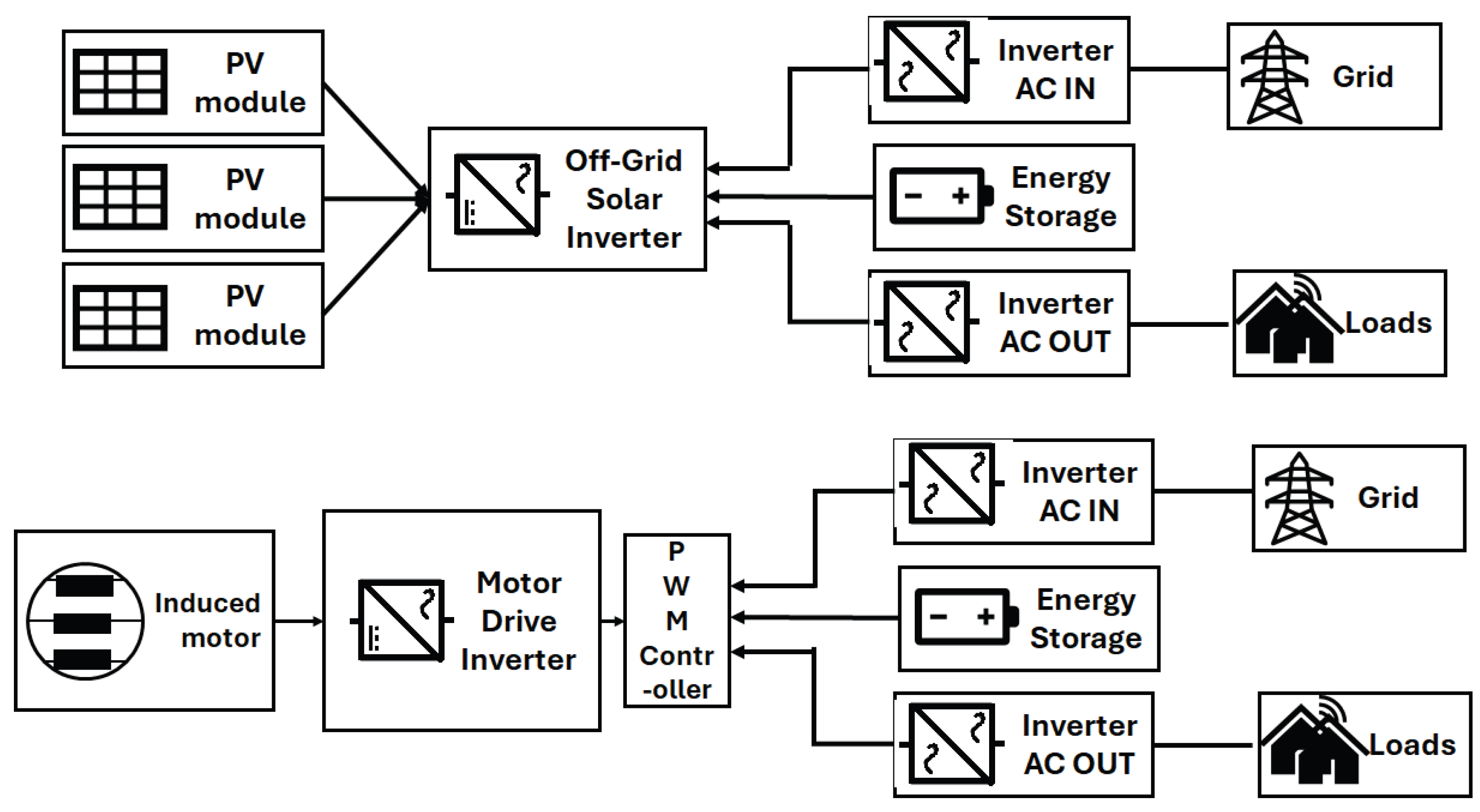
Figure 2.
Diagram illustrating the primary degradation mechanisms in inverters.
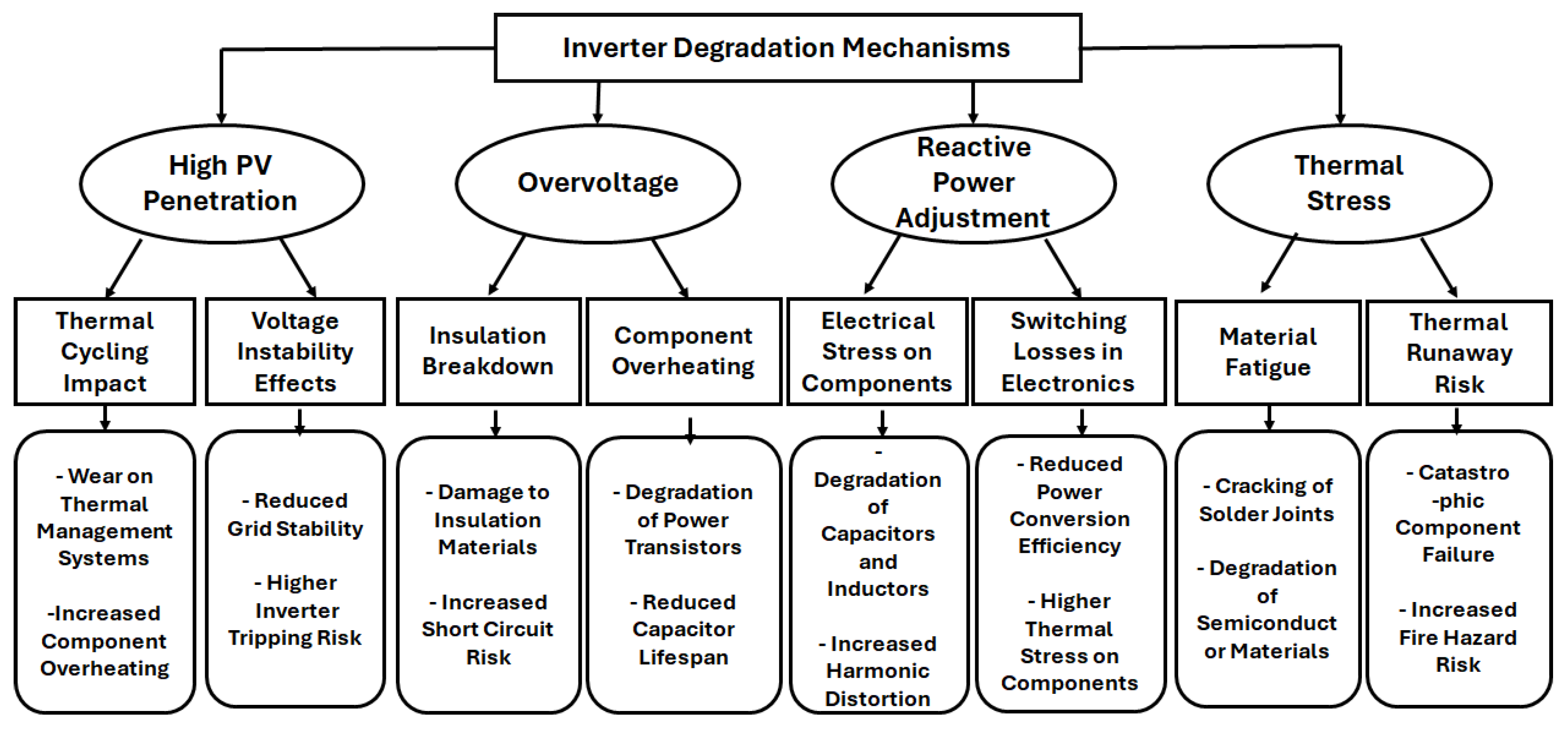
Figure 3.
Modeling results for inverter voltage: the log-normal model provides the most faithful description of the empirical distribution, achieving the lowest information criteria and capturing mild right-skew and tail excursions, whereas symmetric or count-based assumptions underperform. Panels: (a) linear regression—coarse trend estimation; (b) Gaussian—assumes symmetry and underestimates tails; (c) log-normal—best overall fit by AIC/BIC; (d) Gamma—positive support but inferior to log-normal; (e) Poisson—not appropriate for quasi-continuous magnitudes. Main observation: modest but skewed variability; log-normal balances fit and parsimony; linear fits are adequate only for trend depiction. Abbreviations: AIC, Akaike Information Criterion; BIC, Bayesian Information Criterion.
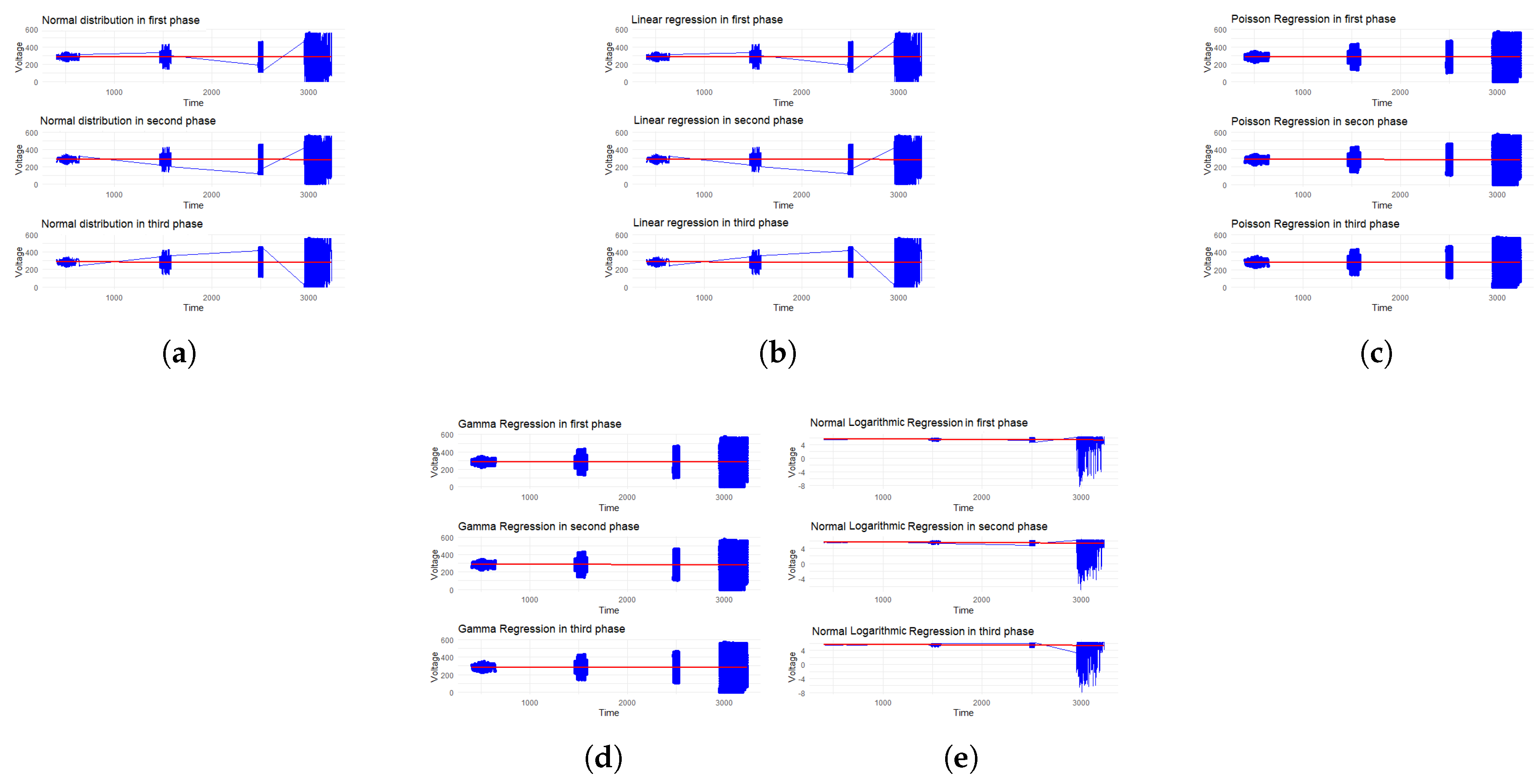
Figure 4.
Modeling results for inverter current: higher short-term volatility and intermittent bursts than voltage. The log-normal model consistently attains the lowest AIC/BIC and accommodates right-tailed fluctuations. Panels: (a) linear regression—captures mean shifts but smooths bursts; (b) Gaussian—symmetric fit that under-represents heavy episodes; (c) log-normal—best overall fit; (d) Gamma—reasonable for positive data yet does not outperform log-normal; (e) Poisson—unsuitable for approximately continuous current magnitudes (non-meaningful information criteria).
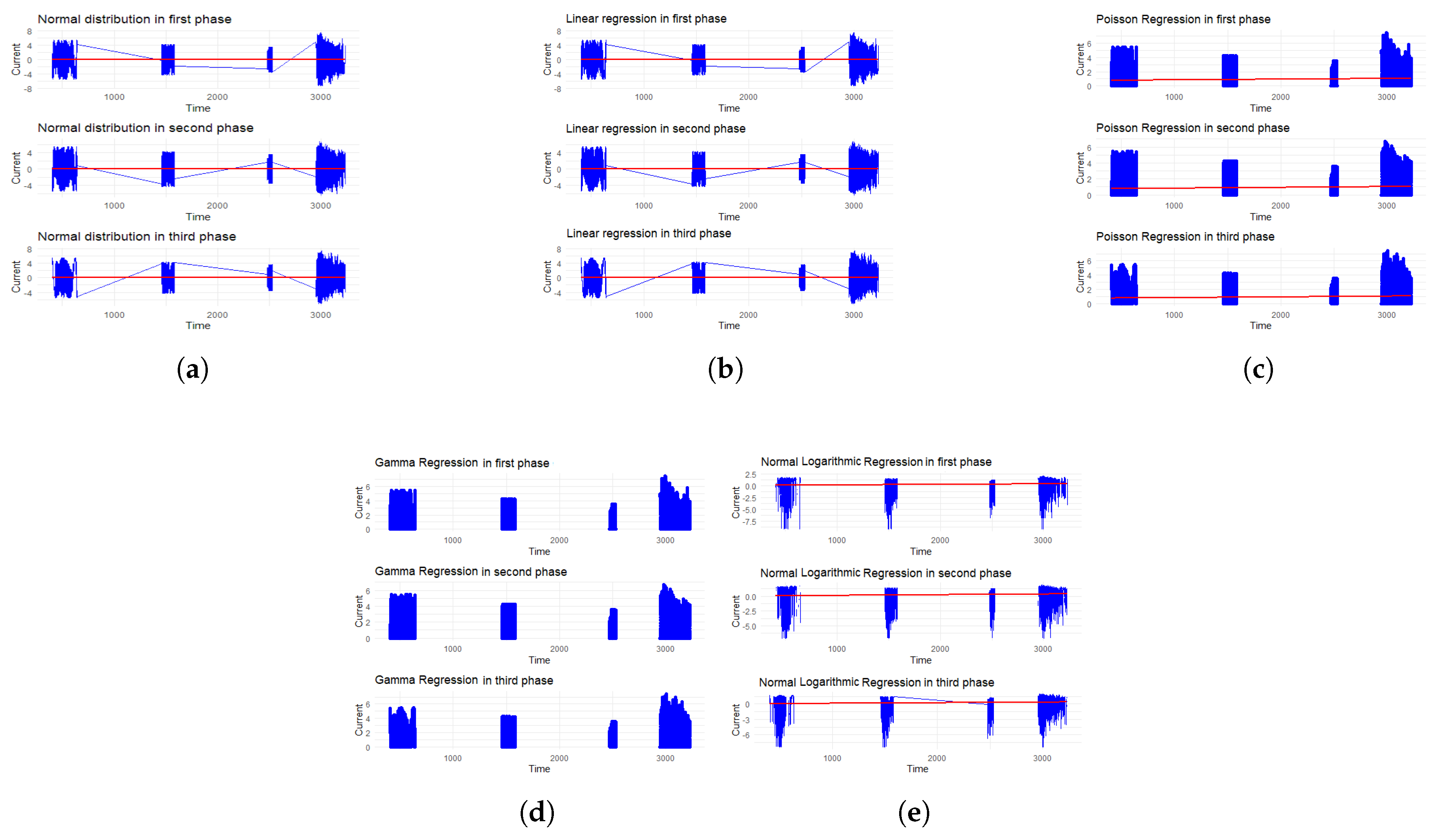
Figure 5.
Modeling results for inverter active power: most dynamic signal, reflecting both operating demand and condition. The log-normal model offers the best overall description (lowest AIC/BIC), capturing skew and intermittent surges; linear regression reflects slow envelope shifts, while Gaussian and Gamma under-capture extremes. Panels: (a) linear—coarse trend depiction only; (b) Gaussian—symmetric fit; (c) log-normal—best overall fit; (d) Gamma—positive-support alternative, inferior by AIC/BIC; (e) Poisson—count model not applicable to quasi-continuous values.
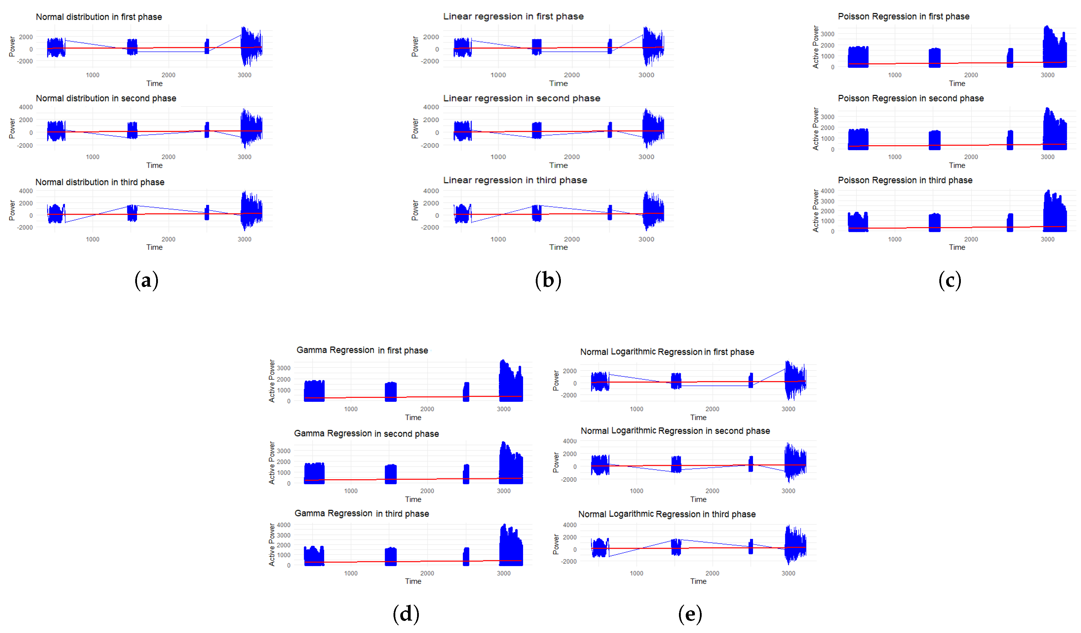
Figure 6.
Schematic of the microgrid illustrating key components involved in voltage regulation.
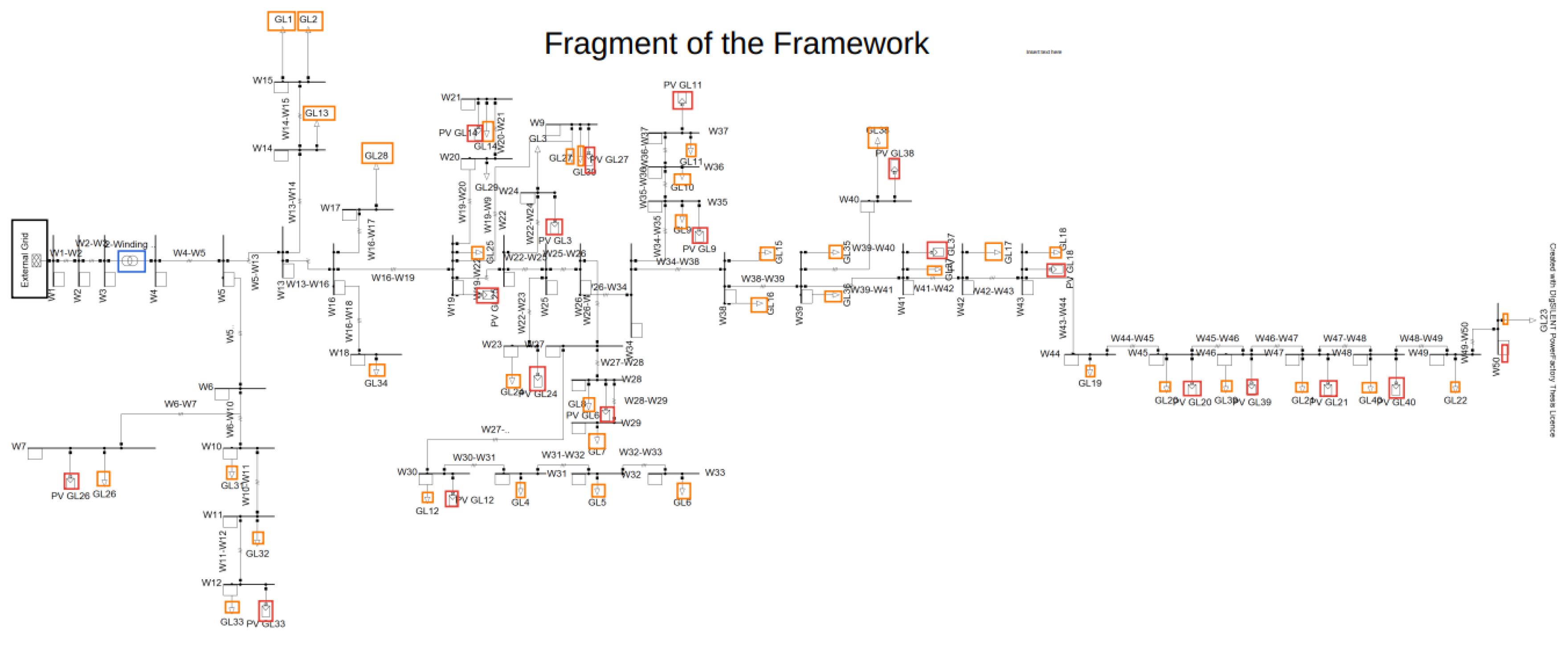
Figure 7.
Waveforms of active and reactive power along with voltage levels in the microgrid.
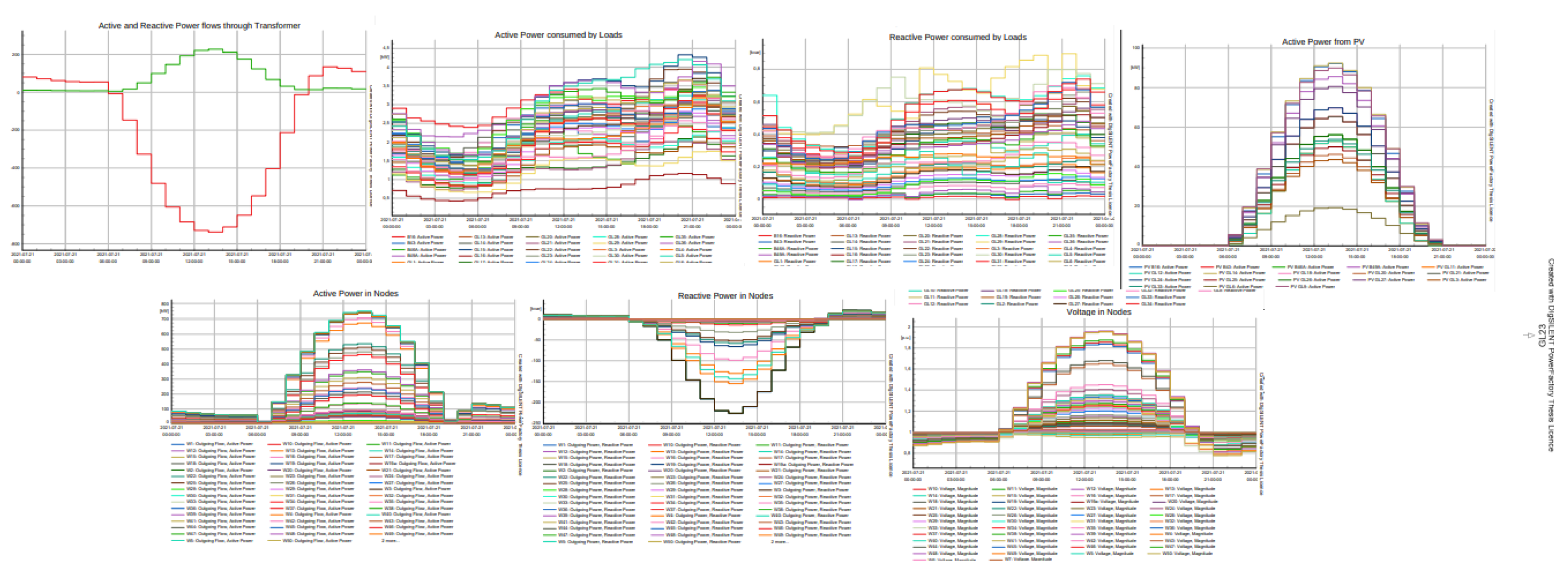
Table 1.
Degradation Mechanisms for Induction Motor Inverters.
| Degradation Mechanism | Causes | Negative Effects |
|---|---|---|
| Thermal Overload [7] | Excessive current due to voltage imbalance or overloading |
Insulation degradation and reduced motor lifespan |
| Bearing Wear [8] | Mechanical stress from misalignment or vibration |
Increased friction, overheating, and eventual motor failure |
| Electrical Insulation Breakdown [9] |
High voltage spikes or harmonics |
Short circuits and reduced motor efficiency |
| Rotor Bar [10] | Cyclic mechanical stress and thermal cycling |
Reduced torque and motor performance |
Table 2.
AIC/BIC comparison of statistical models for voltage across three phases. Lower values indicate better fit. Poisson is included for completeness but is inapplicable to quasi-continuous magnitudes.
Table 2.
AIC/BIC comparison of statistical models for voltage across three phases. Lower values indicate better fit. Poisson is included for completeness but is inapplicable to quasi-continuous magnitudes.
| Model | Phase | Min | Max | Average | AIC | BIC |
|---|---|---|---|---|---|---|
| Linear | 1 | -2.288 | 573.339 | 283.412 | 2854100 | 2854132 |
| 2 | -2.088 | 573.202 | 283.468 | 2847739 | 2847770 | |
| 3 | -2.312 | 573.172 | 283.746 | 2853894 | 2853925 | |
| Normal | 1 | -2.288 | 573.339 | 283.412 | 2889722 | 2889753 |
| 2 | -2.088 | 573.202 | 283.468 | 2888268 | 2888299 | |
| 3 | -2.312 | 573.172 | 283.746 | 2889556 | 2889588 | |
| Log-Normal | 1 | -2.288 | 573.339 | 283.412 | 447315.4 | 447346.4 |
| 2 | -2.088 | 573.202 | 283.468 | 541018.1 | 541049.2 | |
| 3 | -2.312 | 573.172 | 283.746 | 521441.3 | 521472.4 | |
| Gamma | 1 | 1e-06 | 573.339 | 283.429 | 3102113 | 3102144 |
| 2 | 1e-06 | 573.202 | 283.479 | 3085535 | 3085566 | |
| 3 | 1e-06 | 573.172 | 283.760 | 3096033 | 3096064 | |
| Poisson | 1 | 0 | 573.339 | 283.429 | Inf | Inf |
| 2 | 0 | 573.202 | 283.479 | Inf | Inf | |
| 3 | 0 | 573.172 | 283.760 | Inf | Inf |
Table 3.
AIC/BIC comparison of statistical models for current across three phases. Log-normal consistently outperforms other continuous distributions.
Table 3.
AIC/BIC comparison of statistical models for current across three phases. Log-normal consistently outperforms other continuous distributions.
| Model | Phase | Min | Max | Average | AIC | BIC |
|---|---|---|---|---|---|---|
| Linear | A | -7.300 | 7.470 | 0.0005 | 1035254 | 1035285 |
| B | -6.320 | 6.668 | -0.0077 | 1025782 | 1025813 | |
| C | -7.113 | 7.437 | -0.0090 | 1038845 | 1038876 | |
| Normal | A | -7.300 | 7.470 | 0.0005 | 1035254 | 1035285 |
| B | -6.320 | 6.668 | -0.0077 | 1025782 | 1025813 | |
| C | -7.113 | 7.437 | -0.0090 | 1038845 | 1038876 | |
| Log-Normal | A | -7.300 | 7.470 | 0.0005 | 352285.4 | 352314.4 |
| B | -6.320 | 6.668 | -0.0077 | 346475.3 | 346504.4 | |
| C | -7.113 | 7.437 | -0.0090 | 351299.3 | 351328.3 | |
| Gamma | A | 1e-06 | 7.470 | 0.9014 | NA | NA |
| B | 1e-06 | 6.668 | 0.8872 | NA | NA | |
| C | 1e-06 | 7.437 | 0.9052 | NA | NA | |
| Poisson | A | 1e-06 | 7.470 | 0.9014 | Inf | Inf |
| B | 1e-06 | 6.668 | 0.8872 | Inf | Inf | |
| C | 1e-06 | 7.437 | 0.9052 | Inf | Inf |
Table 4.
AIC/BIC comparison of statistical models for power across three phases. Log-normal provides the best fit among evaluated models.
Table 4.
AIC/BIC comparison of statistical models for power across three phases. Log-normal provides the best fit among evaluated models.
| Model | Phase | Min | Max | Average | AIC | BIC |
|---|---|---|---|---|---|---|
| Linear | A | -2976.961 | 3626.644 | 94.839 | 2854100 | 2854132 |
| B | -2583.185 | 3688.165 | 95.983 | 2847739 | 2847770 | |
| C | -2626.442 | 3962.193 | 92.886 | 2853894 | 2853925 | |
| Normal | A | -2976.961 | 3626.644 | 94.839 | 2854100 | 2854132 |
| B | -2583.185 | 3688.165 | 95.983 | 2847739 | 2847770 | |
| C | -2626.442 | 3962.193 | 92.886 | 2853894 | 2853925 | |
| Log-Normal | A | -2976.961 | 3626.644 | 94.839 | 430388.0 | 430419.0 |
| B | -2583.185 | 3688.165 | 95.983 | 523117.1 | 523148.2 | |
| C | -2626.442 | 3962.193 | 92.886 | 506667.8 | 506698.8 | |
| Gamma | A | 1e-06 | 573.339 | 283.429 | 3093952 | 3093983 |
| B | 1e-06 | 573.202 | 283.479 | 3074709 | 3074740 | |
| C | 1e-06 | 573.172 | 283.760 | 3087287 | 3087318 | |
| Poisson | A | 0 | 573.339 | 283.429 | Inf | Inf |
| B | 0 | 573.202 | 283.479 | Inf | Inf | |
| C | 0 | 573.172 | 283.760 | Inf | Inf |
Table 6.
Degradation Mechanisms for PV Inverters.
| Degradation Mechanism | Causes | Negative Effects |
|---|---|---|
| Increased Operating Temperatures | Overvoltage conditions and reactive power adjustments |
Reduced lifespan of heat-sensitive components like capacitors and semiconductors |
| Wear on Components | Frequent reactive power adjustments causing mechanical stress on switching devices (e.g., IGBTs) |
Premature failure of critical components |
| Insulation Breakdown | Voltage stress over time | Increased risk of short circuits and component failures |
| Potential Induced Degradation (PID) |
Stray currents and high system voltages |
Power loss of up to 30 in PV modules |
Disclaimer/Publisher’s Note: The statements, opinions and data contained in all publications are solely those of the individual author(s) and contributor(s) and not of MDPI and/or the editor(s). MDPI and/or the editor(s) disclaim responsibility for any injury to people or property resulting from any ideas, methods, instructions or products referred to in the content. |
© 2025 by the authors. Licensee MDPI, Basel, Switzerland. This article is an open access article distributed under the terms and conditions of the Creative Commons Attribution (CC BY) license (http://creativecommons.org/licenses/by/4.0/).
Copyright: This open access article is published under a Creative Commons CC BY 4.0 license, which permit the free download, distribution, and reuse, provided that the author and preprint are cited in any reuse.


